A Novel Ensemble Approach for Landslide Susceptibility Mapping (LSM) in Darjeeling and Kalimpong Districts, West Bengal, India


Abstract
:
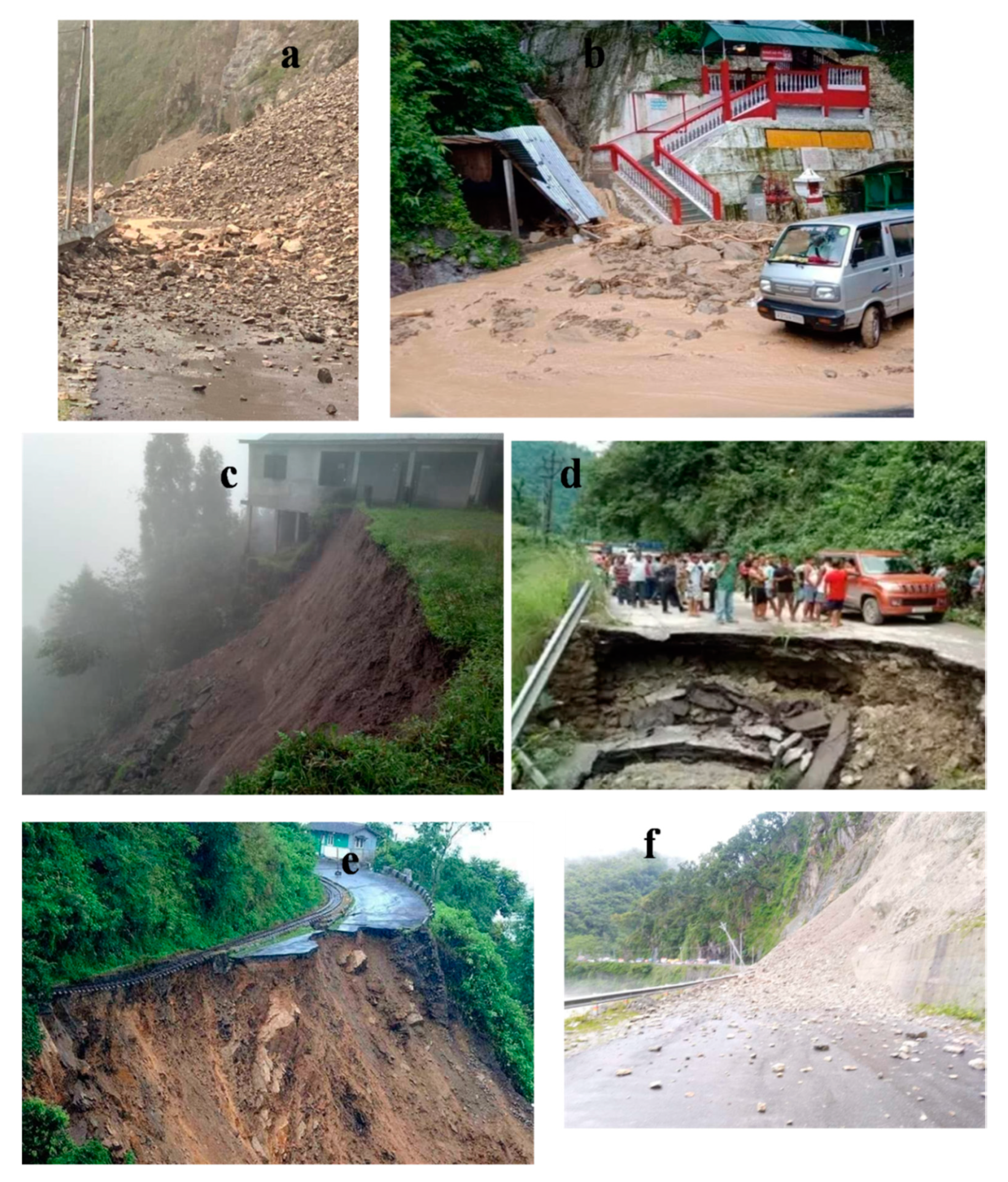
1. Introduction
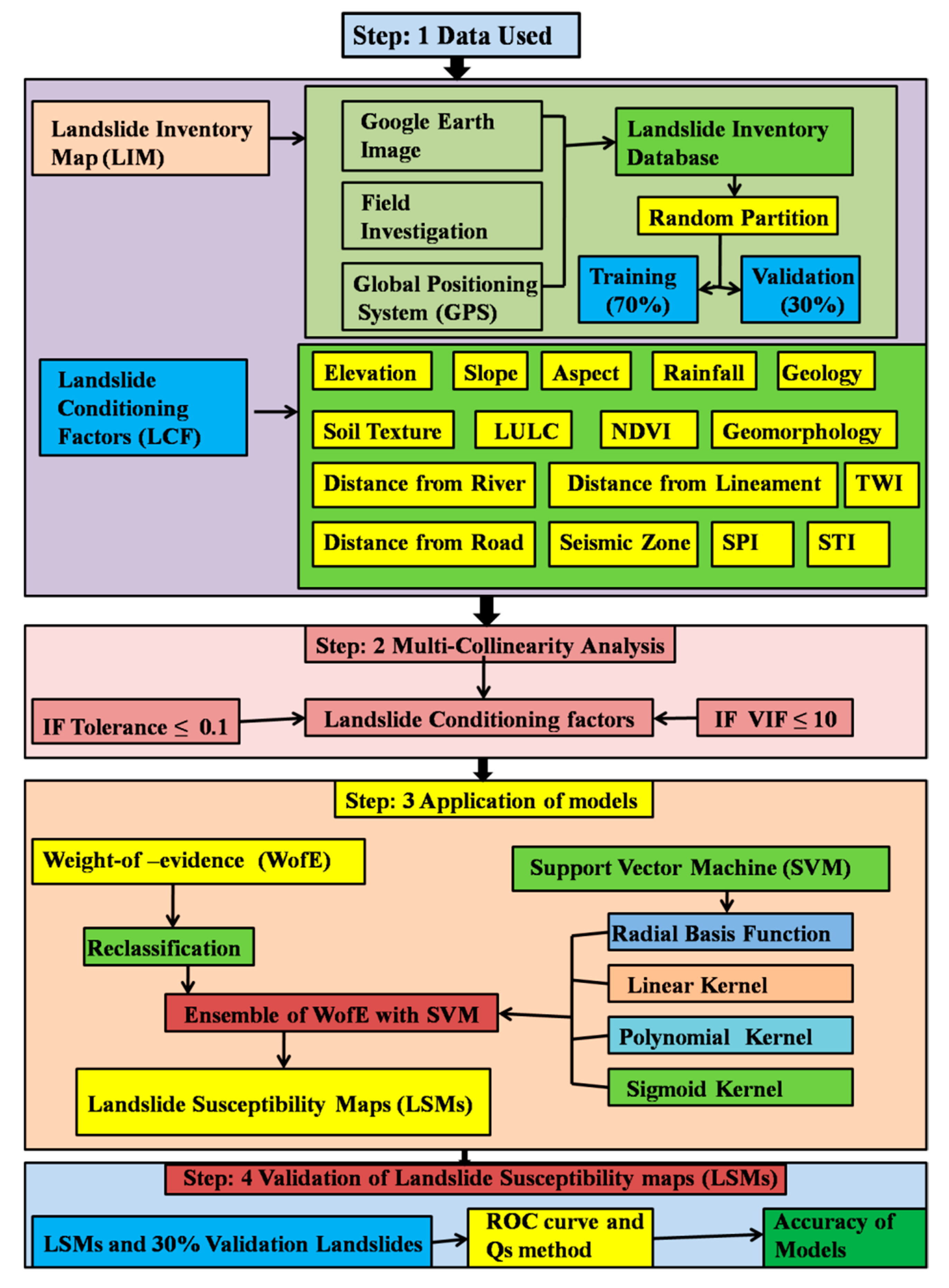
2. Materials and Methods
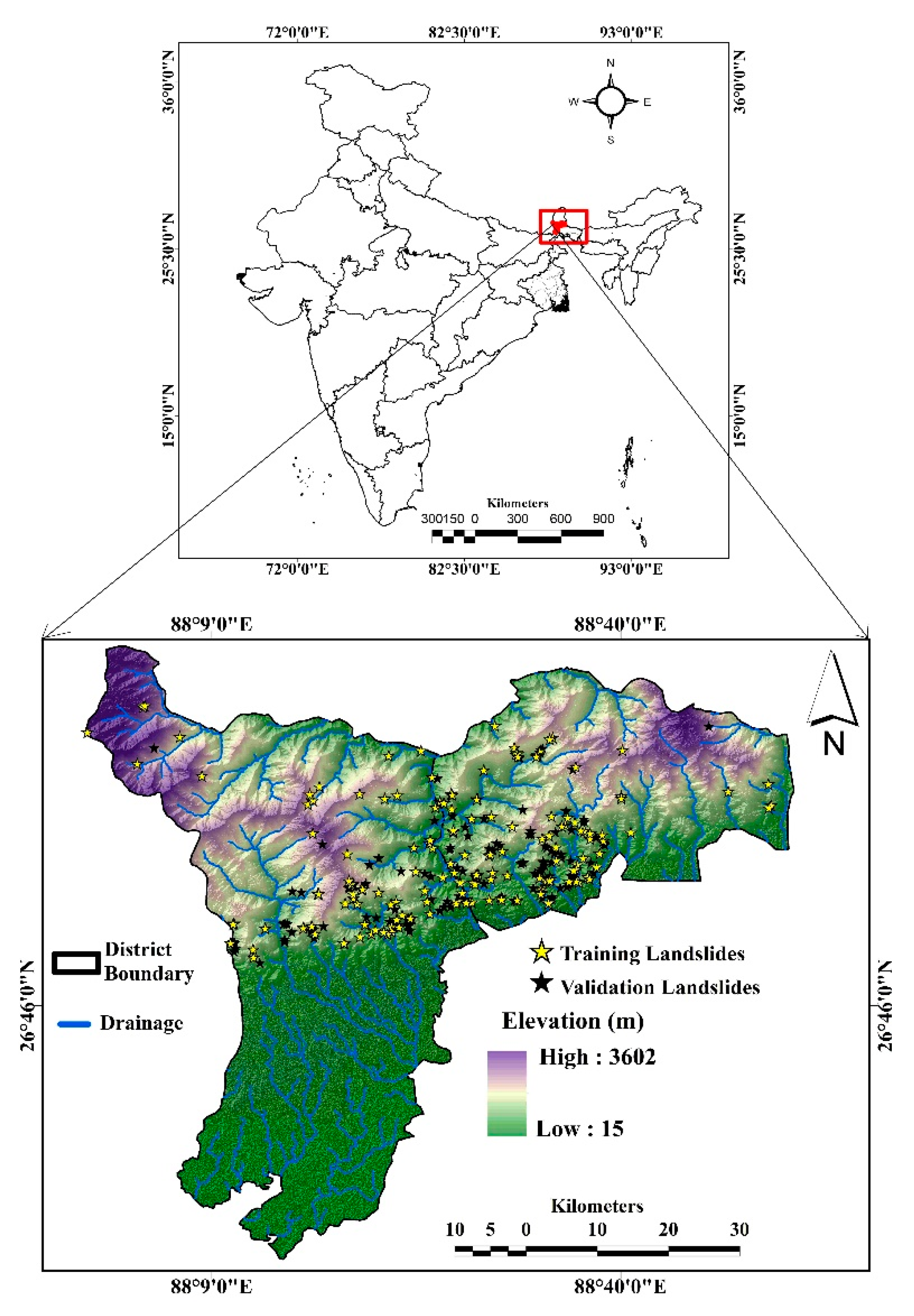
2.1. Study Area
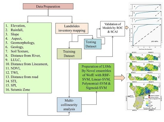
2.2. Methodology
2.3. Data Preparation
2.3.1. Landslide Inventory Dataset
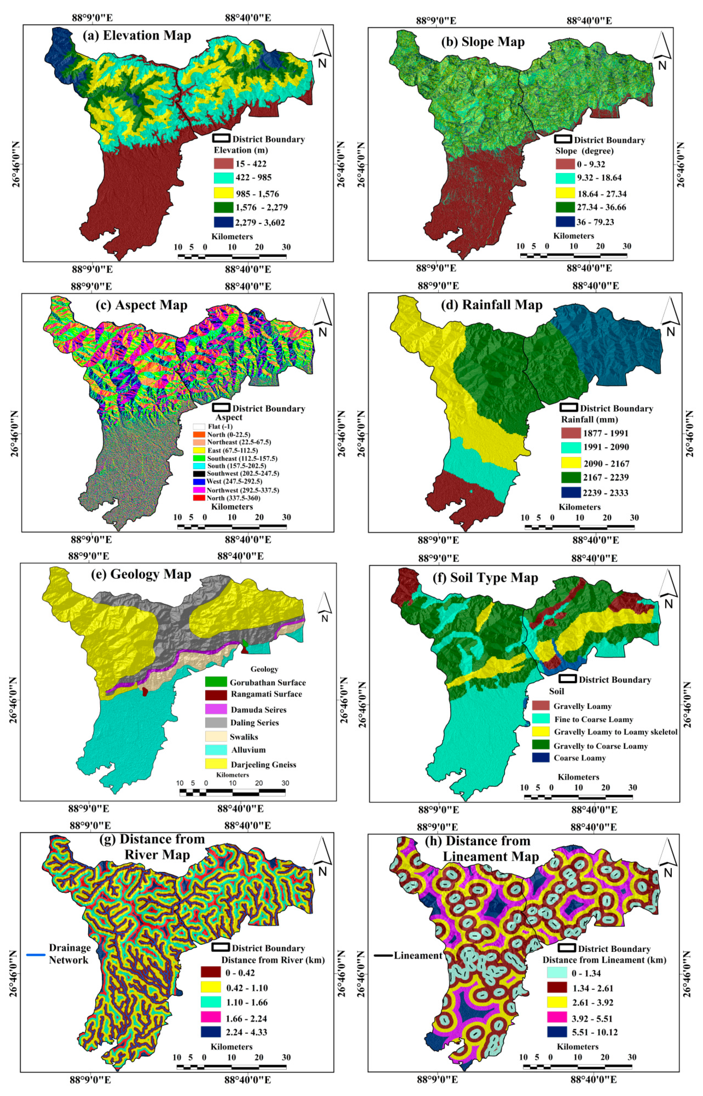
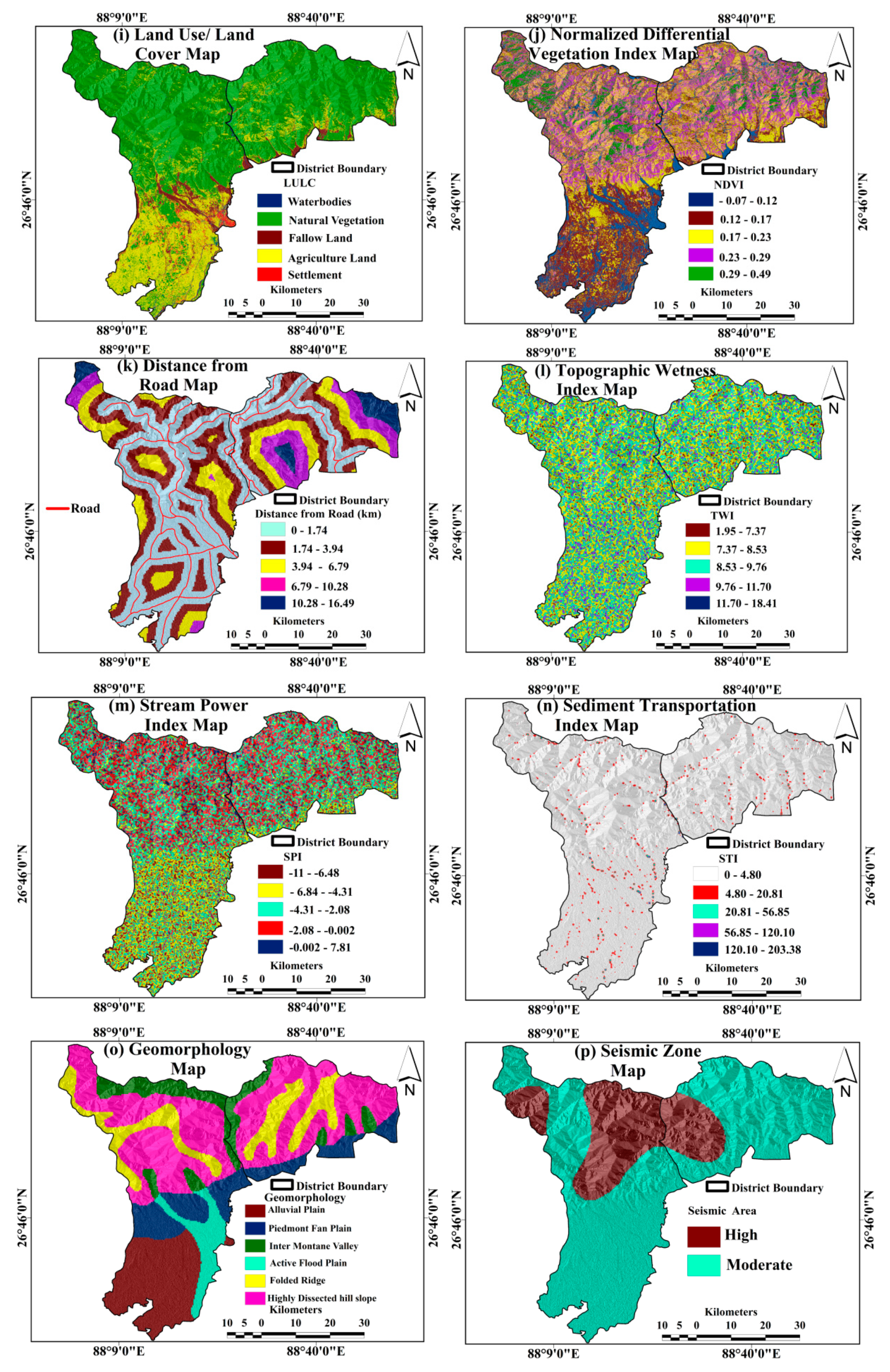
2.3.2. Preparing Effective Factors
2.4. Multicollinearity Analysis
2.5. Models
2.5.1. Weight-of-Evidence (WofE) Model
2.5.2. Support Vector Machine (SVM) Model
3. Results
3.1. Considering the Multicollinearity Analysis of the Effective Factors
3.2. Relationship Between Landslide Location and Effective Factors
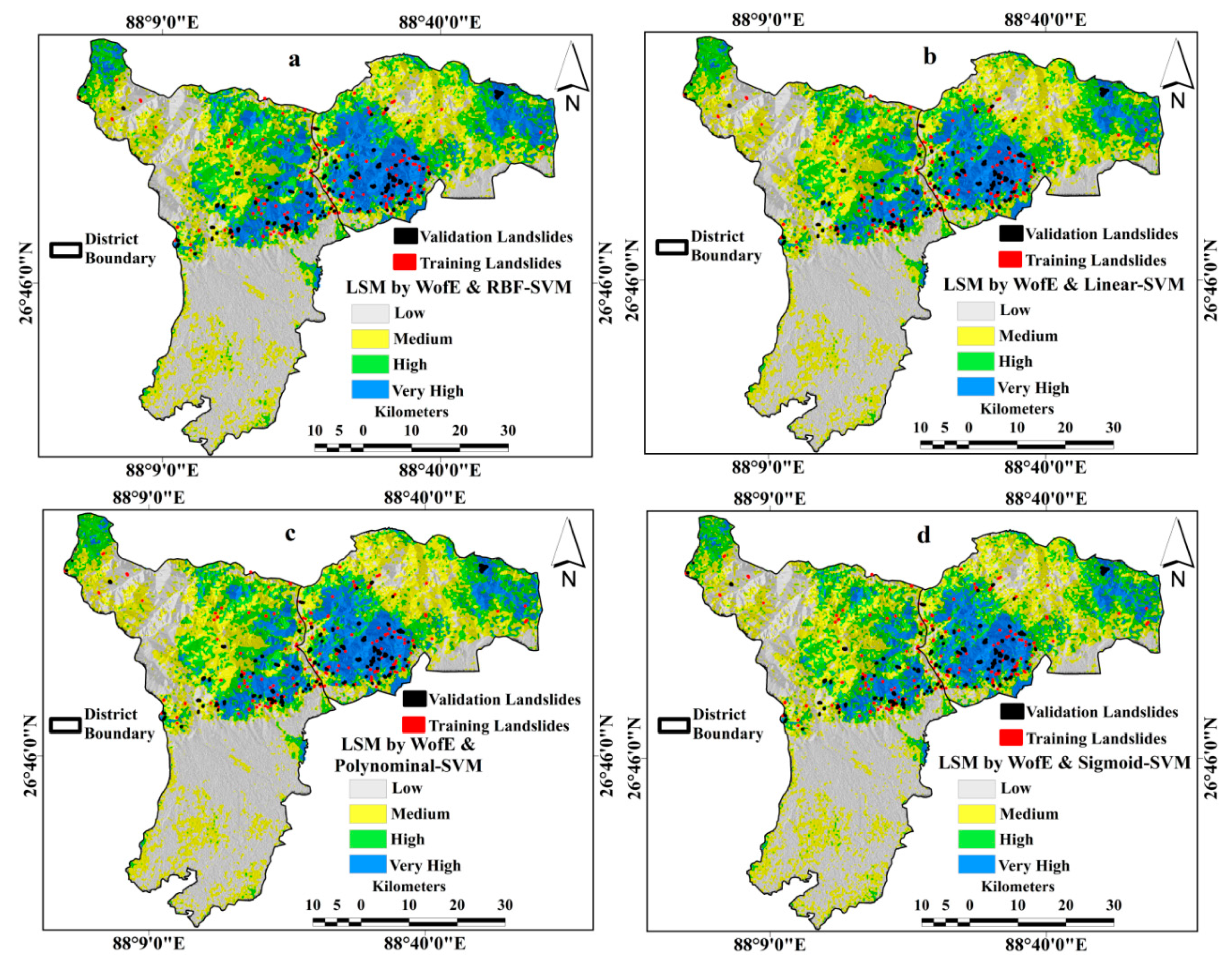
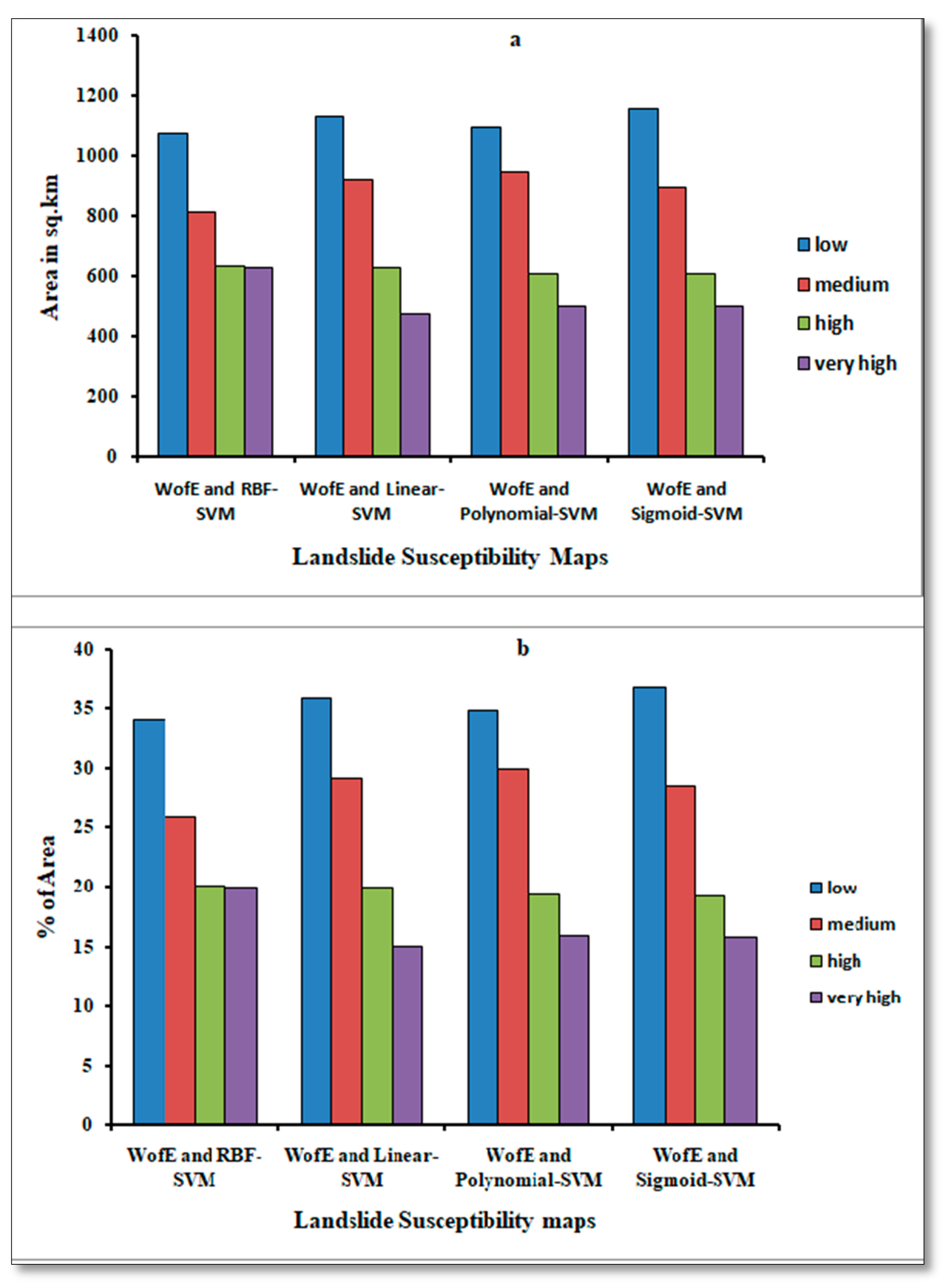
3.3. Landslide Susceptibility Models
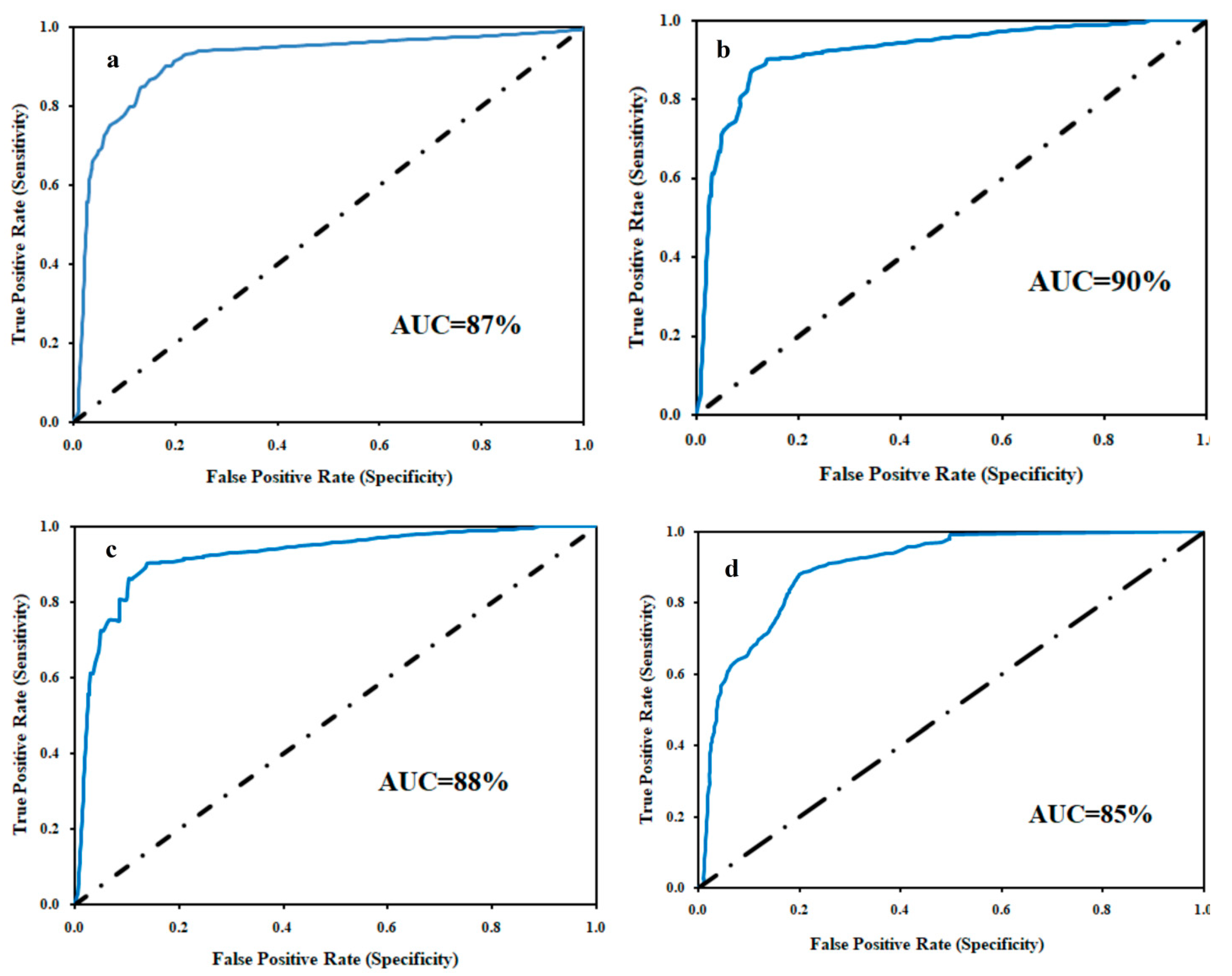
3.4. Validation and Comparison of Models
4. Discussion
5. Conclusions
Author Contributions
Funding
Conflicts of Interest
References
- Bui, D.T.; Tuan, T.A.; Klempe, H.; Pradhan, B.; Revhaug, I. Spatial prediction models for shallow landslide hazards: A comparative assessment of the efficacy of support vector machines, artificial neural networks, kernel logistic regression, and logistic model tree. Landslides 2015, 13, 361–378. [Google Scholar] [CrossRef]
- Cruden, D.M.; Varnes, D.J. Landslide Types and Processes, Transportation Research Board, U.S. National Academy of Sciences. Spec. Rep. 1996, 247, 36–75. [Google Scholar]
- Gerrard, J. The landslide hazard in the Himalayas: Geological control and human action. Geomorphology 1994, 10, 221–230. [Google Scholar] [CrossRef]
- Bhandari, R.K. Landslide hazard zonation: Some thoughts. In Coping with Natural Hazards: Indian Context; Valdiya, K.S., Ed.; Orient Longman: Hyderabad, India, 2004; pp. 134–152. [Google Scholar]
- Panikkar, S.V.; Subramanyan, V.A. geomorphic evaluation of the landslides around Dehradun and Mussoorie, Uttar Pradesh, India. Geomorphology 1996, 15, 169–181. [Google Scholar] [CrossRef]
- Sarkar, S. Landslides in Darjiling Himalayas. Trans. Jpn. Geomorphol. Union 1999, 20, 299–315. [Google Scholar]
- Fan, X.; Scaringi, G.; Domènech, G.; Yang, F.; Guo, X.; Dai, L.; Huang, R. Two multi-temporal datasets that track the enhanced landsliding after the 2008 Wenchuan earthquake. Earth Syst. Sci. Data 2019, 11, 35–55. [Google Scholar] [CrossRef]
- Yilmaz, I. Comparison of landslide susceptibility mapping methodologies for Koyulhisar, Turkey: Conditional probability, logistic regression, artificial neural networks, and support vector machine. Environ. Earth Sci. 2009, 61, 821–836. [Google Scholar] [CrossRef]
- Abedini, M.; Ghasemyan, B.; Mogaddam, M.H.R. Landslide susceptibility mapping in Bijar city, Kurdistan Province, Iran: A comparative study by logistic regression and AHP models. Environ. Earth Sci. 2017, 76, 308. [Google Scholar] [CrossRef]
- Regmi, A.D.; Devkota, K.C.; Yoshida, K.; Pradhan, B.; Pourghasemi, H.R.; Kumamoto, T.; Akgun, A. Application of frequency ratio, statistical index, and weights-of-evidence models and their comparison in landslide susceptibility mapping in Central Nepal Himalaya. Arab. J. Geosci. 2013, 7, 725–742. [Google Scholar] [CrossRef]
- Chawla, A.; Pasupuleti, S.; Chawla, S.; Rao, A.C.S.; Sarkar, K.; Dwivedi, R. Landslide Susceptibility Zonation Mapping: A Case Study from Darjeeling District, Eastern Himalayas, India. J. Indian Soc. Remote Sens. 2019, 47, 497–511. [Google Scholar] [CrossRef]
- Shahabi, H.; Hashim, M. Landslide susceptibility mapping using GIS-based statistical models and Remote sensing data in tropical environment. Sci. Rep. 2015, 5, 15. [Google Scholar] [CrossRef] [PubMed]
- Roy, J.; Saha, S. Landslide susceptibility mapping using knowledge driven statistical models in Darjeeling District, West Bengal, India. Geoenvironmental Disasters 2019, 6, 11. [Google Scholar] [CrossRef]
- Pradhan, B. A comparative study on the predictive ability of the decision tree, support vector machine and neuro-fuzzy models in landslide susceptibility mapping using GIS. Comput. Geosci. 2013, 51, 350–365. [Google Scholar] [CrossRef]
- Pourghasemi, H.R.; Jirandeh, A.G.; Pradhan, B.; Xu, C.; Gokceoglu, C. Landslide susceptibility mapping using support vector machine and GIS at the Golestan Province, Iran. J. Earth Syst. Sci. 2013, 122, 349–369. [Google Scholar] [CrossRef]
- Pham, B.T.; Pradhan, B.; Bui, D.T.; Prakash, I.; Dholakia, M. A comparative study of different machine learning methods for landslide susceptibility assessment: A case study of Uttarakhand area (India). Environ. Model. Softw. 2016, 84, 240–250. [Google Scholar] [CrossRef]
- Goetz, J.; Brenning, A.; Petschko, H.; Leopold, P. Evaluating machine learning and statistical prediction techniques for landslide susceptibility modeling. Comput. Geosci. 2015, 81, 1–11. [Google Scholar] [CrossRef]
- Gravina, T.; Figliozzi, E.; Mari, N.; Schinosa, F.D.L.T. Landslide risk perception in Frosinone (Lazio, Central Italy). Landslides 2016, 14, 1419–1429. [Google Scholar] [CrossRef]
- Pham, B.T.; Bui, D.T.; Prakash, I.; Dholakia, M. Hybrid integration of Multilayer Perceptron Neural Networks and machine learning ensembles for landslide susceptibility assessment at Himalayan area (India) using GIS. Catena 2017, 149, 52–63. [Google Scholar] [CrossRef]
- Pawde, M.B.; Saha, S.S. Geology of Darjeeling Himalaya; GSI: Kolkata, India, 1982. [Google Scholar]
- Pramanik, M.K. Site suitability analysis for agricultural land use of Darjeeling district using AHP and GIS techniques. Model. Earth Syst. Environ. 2016, 2. [Google Scholar] [CrossRef]
- Government of West Bengal. Bureau of Applied Economics and Statistics; Department of Statistics & Programme Implementation, District Statistical Handbook, Government of West Bengal: Kolkata, India, 2013.
- Guzzetti, F.; Reichenbach, P.; Ardizzone, F.; Cardinali, M.; Galli, M. Estimating the quality of landslide susceptibility models. Geomorphology 2006, 81, 166–184. [Google Scholar] [CrossRef]
- Li, Z.; Zhu, Q.; Gold, C. Digital Terrain Modeling: Principles and Methodology; CRC Press: Boca Raton, FL, USA, 2005. [Google Scholar]
- Wentworth, C.K. A simplified method of determining the average slope of land surfaces. Am. J. Sci. 1930, 117, 184–194. [Google Scholar] [CrossRef]
- Burrough, P.A.; McDonell, R.A. Principles of Geographical Information Systems; Oxford University Press: New York, NY, USA, 1998; p. 190. [Google Scholar]
- Bayraktar, H.; Turalioglu, S. A Kriging-based approach for locating a sampling site—In the assessment of air quality. Stoch. Environ. Res. Risk Assess. 2005, 19, 301–305. [Google Scholar] [CrossRef]
- Anderson, C.G.; Maxwell, D.C. Starting a Digitization Center; Elsevier: Amsterdam, The Netherlands, 2004; ISBN 978-1843340737. [Google Scholar]
- Ay, N.; Amari, S.-I. A Novel Approach to Canonical Divergences within Information Geometry. Entropy 2015, 17, 8111–8129. [Google Scholar] [CrossRef]
- Myung, I.J. Tutorial on Maximum Likelihood Estimation. J. Math. Psychol. 2003, 47, 90–100. [Google Scholar] [CrossRef]
- Crippen, R.E. Calculating the vegetation index faster. Remote Sens. Environ. 1990, 34, 71–73. [Google Scholar] [CrossRef]
- Moore, I.D.; Grayson, R.B.; Ladson, A.R. Digital terrain modelling: A review of hydrological, geomorphological, and biological applications. Hydrol. Process. 1991, 5, 3–30. [Google Scholar] [CrossRef]
- Moore, I.D.; Burch, G.J. Physical Basis of the Length Slope Factor in the Universal Soil Loss Equation. Soil Sci. Soc. Am. 1986, 50, 1294–1298. [Google Scholar] [CrossRef]
- Available online: http://0-dx-doi-org.brum.beds.ac.uk/10.2136/sssaj1986.03615995005000050042x (accessed on 21 October 2017).
- O’Brien, R.M. A Caution Regarding Rules of Thumb for Variance Inflation Factors. Qual. Quant. 2007, 41, 673–690. [Google Scholar] [CrossRef]
- Dormann, C.F.; Elith, J.; Bacher, S.; Buchmann, C.; Carl, G.; Carré, G.; Lautenbach, S. Collinearity: A review of methods to deal with it and a simulation study evaluating their performance. Ecography 2012, 36, 27–46. [Google Scholar] [CrossRef]
- Wang, H.; Wang, G.; Wang, F.; Sassa, K.; Chen, Y. Probabilistic modeling of seismically triggered landslides using Monte Carlo simulations. Landslide 2008, 5, 387–395. [Google Scholar] [CrossRef]
- Mohammady, M.; Pourghasemi, H.R.; Pradhan, B. Landslide susceptibility mapping at Golestan Province, Iran: A comparison between frequency ratio, Dempster-Shafer, and weights-ofevidence models. J. Asian Earth Sci. 2012, 61, 221–236. [Google Scholar] [CrossRef]
- Bonham-Carter, G.F. Geographic information systems for geoscientists: Modeling with GIS. In Computer Methods in the Geosciences; Bonham-Carter, F., Ed.; Pergamon: Oxford, UK, 1994; p. 398. [Google Scholar]
- Dahal, R.K.; Hasegawa, S.; Nonomura, A.; Yamanaka, M.; Dhakal, S.; Paudyal, P. Predictive modeling of rainfall-induced landslide hazard in the Lesser Himalaya of Nepal based on weights-of evidence. Geomorphology 2008, 102, 496–510. [Google Scholar] [CrossRef]
- Dahal, R.K.; Hasegawa, S.; Nonomura, A.; Yamanaka, M.; Masuda, T.; Nishino, K. GIS-based weights-of-evidence modeling of rainfall-induced landslides in small catchments for landslide susceptibility mapping. Environ. Geol. 2008, 54, 314–324. [Google Scholar] [CrossRef]
- Wan, S.; Lei, T.C. A knowledge-based decision support system to analyze the debris-flow problems at Chen-Yu-Lan River, Taiwan. Knowl. Based Syst. 2009, 22, 580–588. [Google Scholar] [CrossRef]
- Yao, X.; Tham, L.; Dai, F. Landslide susceptibility mapping based on support vector machine: A case study on natural slopes of Hong Kong, China. Geomorphology 2008, 101, 572–582. [Google Scholar] [CrossRef]
- Marjanovic, M.; Kovacevic, M.; Bajat, B.; Vozenilek, V. Landslide susceptibility assessment using SVM machine learning algorithm. Eng. Geol. 2011, 123, 225–234. [Google Scholar] [CrossRef]
- Tehrany, M.S.; Pradhan, B.; Jebu, M.N. A comparative assessment between object and pixel-based classification approaches for land use/land cover mapping using SPOT 5 imagery. Geocarto Int. 2013, 29, 1–19. [Google Scholar] [CrossRef]
- Tien Bui, D.; Pradhan, B.; Lofman, O.; Revhaug, I. Landslide susceptibility assessment in Vietnam using support vector machines, decision tree, and Naïve Bayes Models. Math. Probl. Eng. 2012, 2012, 1–26. [Google Scholar] [CrossRef] [Green Version]
- Cortes, C.; Vapnik, V. Support-vector networks. Mach. Learn. 1995, 20, 273–297. [Google Scholar] [CrossRef]
- Samui, P. Slope stability analysis: A support vector machine approach. Environ. Geol. 2008, 56, 255–267. [Google Scholar] [CrossRef]
- Arabameri, A.; Pradhan, B.; Rezaei, K. Gully erosion zonation mapping using integrated geographically weighted regression with certainty factor and random forest models in GIS. J. Environ. Manag. 2019, 232, 928–942. [Google Scholar] [CrossRef]
- Arabameri, A.; Pradhan, B.; Rezaei, K. Spatial prediction of gully erosion using ALOS PALSAR data and ensemble bivariate and data mining models. Geosci. J. 2019, 23, 1–18. [Google Scholar] [CrossRef]
- Arabameri, A.; Cerda, A.; Tiefenbacher, J.P. Spatial pattern analysis and prediction of gully erosion using novel hybrid model of entropy-weight of evidence. Water 2019, 11, 1129. [Google Scholar] [CrossRef] [Green Version]
- Arabameri, A.; Pradhan, B.; Rezaei, K.; Conoscenti, C. Gully erosion susceptibility mapping using GISbased multi-criteria decision analysis techniques. Catena 2019, 180, 282–297. [Google Scholar] [CrossRef]
- Arabameri, A.; Rezaei, K.; Cerda, A.; Lombardo, L.; Rodrigo-Comino, J. GIS-based groundwater potential mapping in Shahroud plain, Iran. A comparison among statistical (bivariate and multivariate), data mining and MCDM approaches. Sci. Total Environ. 2019, 658, 160–177. [Google Scholar] [CrossRef]
- Arabameri, A.; Pourghasemi, H.R.; Yamani, M. Applying different scenarios for landslide spatial modeling using computational intelligence methods. Environ. Earth Sci. 2017, 76, 832. [Google Scholar] [CrossRef]
- Arabameri, A.; Pradhan, B.; Rezaei, K.; Sohrabi, M.; Kalantari, Z. GIS-based landslide susceptibility mapping using numerical risk factor bivariate model and its ensemble with linear multivariate regression and boosted regression tree algorithms. J. Mt. Sci. 2019, 16, 595–618. [Google Scholar] [CrossRef]
- Arabameri, A.; Pradhan, B.; Rezaei, K.; Saro, L.; Sohrabi, M. An ensemble model for landslide susceptibility mapping in a forested area. Geochem. Int. 2019, 1–18. [Google Scholar] [CrossRef]
- Chung, C.J.F.; Fabbri, A.G. Validation of Spatial Prediction Models for Landslide Hazard Mapping. Nat. Hazards 2003, 30, 451–472. [Google Scholar] [CrossRef]
- Negnevitsky, M. Artificial Intelligence—A Guide to Intelligent Systems; Addison-Wesley Co.: Boston, MA, USA, 2002; p. 394. [Google Scholar]
- Mallick, J.; Singh, R.K.; Alawadh, M.A.; Islam, S.; Khan, R.A.; Qureshi, M.N. GIS-based landslide susceptibility evaluation using fuzzy-AHP multi-criteria decision-making techniques in the Abha Watershed, Saudi Arabia. Environ. Earth Sci. 2018, 77, 276. [Google Scholar] [CrossRef]
- Feizizadeh, B.; Roodposhti, M.S.; Jankowski, P.; Blaschke, T. A GIS-based extended fuzzy multi-criteria evaluation for landslide susceptibility mapping. Comput. Geosci. 2014, 73, 208–221. [Google Scholar] [CrossRef] [PubMed] [Green Version]
- Park, S.; Choi, C.; Kim, B.; Kim, J. Landslide susceptibility mapping using frequency ratio, analytic hierarchy process, logistic regression, and artificial neural network methods at the Inje area, Korea. Environ. Earth Sci. 2012, 68, 1443–1464. [Google Scholar] [CrossRef]
- Bijukchhen, S.M.; Kayastha, P.; Dhital, M.R. A comparative evaluation of heuristic and bivariate statistical modelling for landslide susceptibility mappings in Ghurmi–DhadKhola, east Nepal. Arab. J. Geosci. 2012, 6, 2727–2743. [Google Scholar] [CrossRef]
- Pradhan, B.; Youssef, A.M. Manifestation of remote sensing data and GIS on landslide hazard analysis using spatial-based statistical models. Arab. J. Geosci. 2009, 3, 319–326. [Google Scholar] [CrossRef]
- Ozdemir, A.; Altural, T. A comparative study of frequency ratio, weights of evidence and logistic regression methods for landslide susceptibility mapping: Sultan Mountains, SW Turkey. J. Asian Earth Sci. 2013, 64, 180–197. [Google Scholar] [CrossRef]
- Arabameri, A.; Yamani, M.; Pradhan, B.; Melesse, A.; Shirani, K.; Bui, D.T. Novel ensembles of COPRAS multi-criteria decision-making with logistic regression, boosted regression tree, and random forest for spatial prediction of gully erosion susceptibility. Sci. Total Environ. 2019, 688, 903–916. [Google Scholar] [CrossRef]
- Tien Bui, D.; Hoang, N.D.; Martínez-Álvarez, F.; Ngo, P.T.T.; Hoa, P.V.; Pham, T.D.; Samui, P.; Costache, R. A novel deep learning neural network approach for predicting flash flood susceptibility: A case study at a high frequency tropical storm area. Sci. Total Environ. 2019. [Google Scholar] [CrossRef]
- Abedini, M.; Tulabi, S. Assessing LNRF, FR, and AHP models in landslide susceptibility mapping index: A comparative study of Nojian watershed in Lorestan province, Iran. Environ. Earth Sci. 2018, 77, 405. [Google Scholar] [CrossRef]
- Haneberg, W.C.; Cole, W.F.; Kasali, G. High-resolution lidar-based landslide hazard mapping and modeling, UCSF Parnassus Campus, San Francisco, USA. Bull. Eng. Geol. Environ. 2009, 68, 263–276. [Google Scholar] [CrossRef]
- Nichol, J.E.; Shaker, A.; Wong, M.S. Application of high-resolution stereo satellite images to detailed landslide hazard assessment. Geomorphology 2006, 76, 68–75. [Google Scholar] [CrossRef]


| Age | Series | Lithological Characteristics |
|---|---|---|
| Recent (Holocene) Pleistocene | Sub-aerial formations (soil, alluvia, colluvial) Raised Terraces | Younger flood plain deposits of the rivers composed of sand, gravel, pebble, etc. and soil covering the rocks sandy, clay, gravel, pebble, boulders etc. representing older fluvial deposits |
| Miocene | Siwalik | Micaceous sandstones with slaty bands, seams of graphitic coal, silts and minor bands of limestone |
| Permian | Damuda Series (Lower Gondwana) | Quartzitic sandstones with slaty bands, carbonaceous shales, seams of graphitic coal, lamprophyre sills and minor bands of limestone |
| Precambrian | 1) Darjeeling gneiss 2) Daling gneiss | Golden-silvery micaschists; Carbonaceousmicaschists; Granatiferousmicaschists and coarse grained gneisses. Slates (greenish to grey with perfect slaty cleavage). Phyllites surrounded by pebbles of quartz, Chlorite-schists with bands of grilty schist’s injected with gneiss (crinkled). Granites, pagmatites’s and quartz veins, with tourmaline and iron as accessories |
| Sl. No. | Parameters | Data Used & Scale | Sources of Data Types | Techniques | References |
|---|---|---|---|---|---|
| 1 | Elevation | DEM 30 m × 30 | U.S Geological Survey | 30 m × 30 m digital elevation model | [24] |
| 2 | Slope | DEM 30 m × 30 | U.S Geological Survey | N=No. of Contour Cutting; i=Contour Interval | [25] |
| 3 | Aspect | DEM 30 m × 30 | U.S Geological Survey | Where, dz/dx= ((c+2f+i)−(a+2d+g))/8 dz/dy=((g+2h+i)−(a+2b+c))/8 Here, a to i indicates the cell value of 3*3 window. | [26] |
| 4 | Rainfall | Annual average rainfall data of different stations in the last 5 years | Indian Metrological Department (IMD) | Kriging Interpolation method | [27] |
| 5 | Geology | Reference geological map 1: 50,000 | Geological Survey of India | Digitization process | [28] |
| 6 | Soil | Reference district soil map 1: 50,000 | National Bureau of Soil Survey and Land Use Planning | Digitization process | [28] |
| 7 | Distance from River | Reference Topomap 1: 50,000 | Survey of India | Euclidian Distance Buffering | [29] |
| 8 | Distance from Lineament | Reference sheet of Lineament 30 m × 30 | “https://bhuvan-vec2.nrsc.gov.in/bhuvan/wms” | Euclidian Distance Buffering | [29] |
| 9 | Land use/land cover (LULC) | Landsat 8 OLI/TIRS 30 m × 30 | U.S Geological Survey | Maximum likelihood Classification | [30] |
| 10 | Normalized differential vegetation index (NDVI) | Landsat 8 OLI/TIRS 30 m × 30 | U.S Geological Survey | Where NIR is the near infrared band or band 4 and IR is the infrared band or band 3. | [31] |
| 11 | Distance from road | Reference Topomap 1: 50,000 | Survey of India | Euclidian Distance Buffering | [29] |
| 12 | Topographic wetness index (TWI) | DEM 30 m×30 1: 50,000 | U.S Geological Survey | Where α is the cumulative upslope area draining through a point (per unit contour length), and β is the slope gradient (in degree). | [32]. |
| 13 | Stream power index (SPI) | DEM 30 m × 30 1: 50,000 | U.S Geological Survey | Where AS is the upstream contributing area and β is the slope gradient (in degrees) | [32]. |
| 14 | Sediment transportation index (STI) | DEM 30 m × 30 | U.S Geological Survey | Where, As, is the specific catchment area; ‘B’ is the local slope gradient in degrees; m is usually set to 0.4, ‘n’, is usually set to 0.0896 | [33] |
| 15 | Geomorphology | Reference sheet 1: 50,000 | “https://bhuvan-vec2.nrsc.gov.in/bhuvan/wms” | Digitization process | [27] |
| 16 | Seismic zone map | Last 200 years point data of earthquake 30 m × 30 | National Centre for Seismology, New Delhi, India | Gridding and Interpolation (Inverse distance weight method) | [11] |
| Kernel Types | Equations | Kernel Parameters |
|---|---|---|
| Radial Basis Function (RBF) | ||
| Linear kernel | --- | |
| Polynomial kernel | ||
| Sigmoid kernel |
| Landslide Conditioning Factors | Collinearity Statistics | |
|---|---|---|
| Tolerance | VIF | |
| Rainfall | 0.446 | 2.241 |
| Elevation | 0.520 | 1.924 |
| Slope | 0.824 | 1.213 |
| Aspect | 0.672 | 1.488 |
| Geology | 0.688 | 1.453 |
| Soil | 0.756 | 1.323 |
| Distance from River | 0.570 | 1.753 |
| Distance from lineament | 0.773 | 1.294 |
| Distance from Road | 0.499 | 2.003 |
| Land use/land cover (LULC) | 0.754 | 1.326 |
| Normalized differential vegetation index (NDVI) | 0.757 | 1.320 |
| Topographic wetness index (TWI) | 0.677 | 1.477 |
| Stream power index (SPI) | 0.684 | 1.461 |
| Sediment transportation index (STI) | 0.768 | 1.302 |
| Geomorphology | 0.789 | 1.268 |
| Seismic zone | 0.618 | 1.618 |
| Rainfall (mm) | Pixels | % of Pixels | Landslide Pixels | % of Pixels | W+ | W− | C | S2W+ | S2W− | S© | W |
|---|---|---|---|---|---|---|---|---|---|---|---|
| 1877.38–1991.97 | 322590 | 8.784 | 0 | 0.000 | 0.000 | 0.092 | 0.000 | 0.000 | 0.000 | 0.000 | 0.000 |
| 1991.97–2090.54 | 289906 | 7.894 | 0 | 0.000 | 0.000 | 0.082 | 0.000 | 0.000 | 0.000 | 0.000 | 0.000 |
| 2090.45–2167.44 | 944320 | 25.712 | 393 | 7.895 | −1.182 | 0.215 | −1.397 | 0.003 | 0.000 | 0.053 | −26.580 |
| 2167.44–2239.06 | 1333493 | 36.309 | 3670 | 73.684 | 0.709 | −0.885 | 1.594 | 0.000 | 0.001 | 0.032 | 49.504 |
| 2239.06–2333.96 | 782357 | 21.302 | 918 | 18.421 | −0.145 | 0.036 | −0.182 | 0.001 | 0.000 | 0.037 | −4.963 |
| Slope (Degree) | |||||||||||
| 0–9.32 | 1175818 | 32.015 | 92 | 1.847 | −2.854 | 0.368 | −3.222 | 0.011 | 0.000 | 0.105 | −30.614 |
| 9.32–18.64 | 665098 | 18.109 | 571 | 11.464 | −0.458 | 0.078 | −0.536 | 0.002 | 0.000 | 0.044 | −12.044 |
| 18.44–27.34 | 813896 | 22.161 | 1172 | 23.529 | 0.060 | −0.018 | 0.078 | 0.001 | 0.000 | 0.033 | 2.326 |
| 27.34–36.66 | 694449 | 18.909 | 1579 | 31.700 | 0.518 | −0.172 | 0.690 | 0.001 | 0.000 | 0.030 | 22.622 |
| 36.66–79.23 | 323404 | 8.806 | 1567 | 31.460 | 1.277 | −0.286 | 1.563 | 0.001 | 0.000 | 0.031 | 51.122 |
| Altitude(m) | |||||||||||
| 15–422 | 1351511 | 36.799 | 417 | 8.373 | −1.482 | 0.372 | −1.854 | 0.002 | 0.000 | 0.051 | −36.226 |
| 422 – 985 | 837224 | 22.796 | 2491 | 50.000 | 0.787 | −0.435 | 1.222 | 0.000 | 0.000 | 0.028 | 43.079 |
| 985 –1576 | 738499 | 20.108 | 1005 | 20.173 | 0.003 | −0.001 | 0.004 | 0.001 | 0.000 | 0.035 | 0.115 |
| 1576 – 2279 | 518669 | 14.122 | 839 | 16.844 | 0.176 | −0.032 | 0.209 | 0.001 | 0.000 | 0.038 | 5.509 |
| 2279 – 3602 | 226762 | 6.174 | 230 | 4.610 | −0.293 | 0.017 | −0.309 | 0.004 | 0.000 | 0.068 | −4.572 |
| Aspect | |||||||||||
| Flat(−1) | 1905 | 0.052 | 0 | 0.000 | 0.000 | 0.001 | 0.000 | 0.000 | 0.000 | 0.000 | 0.000 |
| north | 236967 | 6.452 | 39 | 0.788 | −2.104 | 0.059 | −2.163 | 0.025 | 0.000 | 0.160 | −13.495 |
| northeast | 462023 | 12.580 | 363 | 7.289 | −0.546 | 0.059 | −0.605 | 0.003 | 0.000 | 0.055 | −11.098 |
| east | 454970 | 12.388 | 651 | 13.061 | 0.053 | −0.008 | 0.061 | 0.002 | 0.000 | 0.042 | 1.443 |
| southeast | 522200 | 14.219 | 1098 | 22.045 | 0.439 | −0.096 | 0.535 | 0.001 | 0.000 | 0.034 | 15.640 |
| south | 525807 | 14.317 | 1292 | 25.946 | 0.596 | −0.146 | 0.742 | 0.001 | 0.000 | 0.032 | 22.922 |
| southwest | 457236 | 12.450 | 890 | 17.868 | 0.362 | −0.064 | 0.426 | 0.001 | 0.000 | 0.037 | 11.505 |
| west | 378362 | 10.302 | 462 | 9.279 | −0.105 | 0.011 | −0.116 | 0.002 | 0.000 | 0.049 | −2.376 |
| northwest | 419573 | 11.424 | 154 | 3.093 | −1.308 | 0.090 | −1.398 | 0.006 | 0.000 | 0.082 | −17.074 |
| north | 213621 | 5.817 | 31 | 0.630 | −2.223 | 0.054 | −2.277 | 0.032 | 0.000 | 0.179 | −12.718 |
| Geology | |||||||||||
| Swaliks | 1936266 | 52.721 | 3182 | 63.889 | 0.192 | −0.270 | 0.462 | 0.000 | 0.001 | 0.030 | 15.659 |
| Darjeeling Gneiss | 270526 | 7.366 | 692 | 13.889 | 0.635 | −0.073 | 0.709 | 0.001 | 0.000 | 0.041 | 17.273 |
| Daling series | 131471 | 3.580 | 415 | 8.333 | 0.847 | −0.051 | 0.897 | 0.002 | 0.000 | 0.051 | 17.480 |
| Alluvium | 678512 | 18.475 | 0 | 0.000 | 0.000 | 0.205 | 0.000 | 0.000 | 0.000 | 0.000 | 0.000 |
| Damuda series | 655890 | 17.859 | 692 | 13.889 | −0.252 | 0.047 | −0.299 | 0.001 | 0.000 | 0.041 | −7.293 |
| Soil | |||||||||||
| Gravelly-loamy | 274651 | 7.478 | 830 | 16.667 | 0.803 | −0.105 | 0.908 | 0.001 | 0.000 | 0.038 | 23.845 |
| Fine loamy_Coarse Loamy | 1477848 | 40.239 | 1107 | 22.222 | −0.594 | 0.264 | −0.858 | 0.001 | 0.000 | 0.034 | −25.171 |
| Gravelly loamy_LoamySkeletol | 450035 | 12.254 | 1107 | 22.222 | 0.596 | −0.121 | 0.717 | 0.001 | 0.000 | 0.034 | 21.019 |
| Gravelly Loamy_Coarse Loamy | 1404794 | 38.250 | 1660 | 33.333 | −0.138 | 0.077 | −0.214 | 0.001 | 0.000 | 0.030 | −7.131 |
| Coarse Loamy | 65336 | 1.779 | 277 | 5.556 | 1.142 | −0.039 | 1.181 | 0.004 | 0.000 | 0.062 | 19.055 |
| Distance from River (km) | |||||||||||
| 0–0.42 | 1160959 | 31.611 | 1049 | 21.053 | −0.407 | 0.144 | −0.551 | 0.001 | 0.000 | 0.035 | −15.837 |
| 0.42–1.10 | 1291696 | 35.171 | 1966 | 39.474 | 0.116 | −0.069 | 0.184 | 0.001 | 0.000 | 0.029 | 6.356 |
| 1.10–1.66 | 750401 | 20.432 | 1442 | 28.947 | 0.349 | −0.113 | 0.462 | 0.001 | 0.000 | 0.031 | 14.784 |
| 1.66–2.26 | 371677 | 10.120 | 393 | 7.895 | −0.249 | 0.024 | −0.273 | 0.003 | 0.000 | 0.053 | −5.195 |
| 2.26–4.33 | 97931 | 2.666 | 131 | 2.632 | −0.013 | 0.000 | −0.014 | 0.008 | 0.000 | 0.089 | −0.153 |
| Distance from Lineament(km) | |||||||||||
| 0–1.54 | 763490 | 20.788 | 906 | 18.182 | −0.134 | 0.032 | −0.167 | 0.001 | 0.000 | 0.037 | −4.531 |
| 1.54–2.85 | 1093457 | 29.773 | 1019 | 20.455 | −0.376 | 0.125 | −0.501 | 0.001 | 0.000 | 0.035 | −14.243 |
| 2.85–4.20 | 941314 | 25.630 | 1472 | 29.545 | 0.142 | −0.054 | 0.197 | 0.001 | 0.000 | 0.031 | 6.323 |
| 4.20–5.75 | 633142 | 17.239 | 1245 | 25.000 | 0.372 | −0.099 | 0.471 | 0.001 | 0.000 | 0.033 | 14.378 |
| 5.75–10.12 | 241263 | 6.569 | 340 | 6.818 | 0.037 | −0.003 | 0.040 | 0.003 | 0.000 | 0.056 | 0.710 |
| Distance from Road(km) | |||||||||||
| 0–1.74 | 1636028 | 44.546 | 792 | 15.909 | −1.031 | 0.417 | −1.448 | 0.001 | 0.000 | 0.039 | −37.353 |
| 1.74–3.94 | 988335 | 26.911 | 906 | 18.182 | −0.393 | 0.113 | −0.506 | 0.001 | 0.000 | 0.037 | −13.754 |
| 3.94–6.72 | 589253 | 16.044 | 906 | 18.182 | 0.125 | −0.026 | 0.151 | 0.001 | 0.000 | 0.037 | 4.109 |
| 6.72–10.22 | 316628 | 8.621 | 1472 | 29.545 | 1.235 | −0.260 | 1.495 | 0.001 | 0.000 | 0.031 | 48.066 |
| 10.22–16.49 | 142420 | 3.878 | 906 | 18.182 | 1.550 | −0.161 | 1.711 | 0.001 | 0.000 | 0.037 | 46.466 |
| Land use/Land cover | |||||||||||
| Water bodies | 40427 | 1.101 | 0 | 0.000 | 0.000 | 0.011 | 0.000 | 0.000 | 0.000 | 0.000 | 0.000 |
| Vegetation | 2650294 | 72.163 | 1119 | 22.464 | −1.168 | 1.027 | −2.195 | 0.001 | 0.000 | 0.034 | −64.607 |
| Fallow land | 168382 | 4.585 | 1624 | 32.609 | 1.970 | −0.348 | 2.318 | 0.001 | 0.000 | 0.030 | 76.445 |
| Agricultural land | 763256 | 20.782 | 2238 | 44.928 | 0.773 | −0.364 | 1.137 | 0.000 | 0.000 | 0.029 | 39.858 |
| Settlement | 50306 | 1.370 | 0 | 0.000 | 0.000 | 0.014 | 0.000 | 0.000 | 0.000 | 0.000 | 0.000 |
| Normalized differential vegetation index (NDVI) | |||||||||||
| −0.07–0.12 | 442450 | 12.047 | 1399 | 28.093 | 0.849 | −0.202 | 1.050 | 0.001 | 0.000 | 0.032 | 33.271 |
| 0.12–0.17) | 972514 | 26.480 | 1421 | 28.523 | 0.074 | −0.028 | 0.103 | 0.001 | 0.000 | 0.031 | 3.270 |
| 0.17–0.23) | 997257 | 27.154 | 1312 | 26.336 | −0.031 | 0.011 | −0.042 | 0.001 | 0.000 | 0.032 | −1.297 |
| 0.23–0.29 | 816592 | 22.234 | 618 | 12.411 | −0.584 | 0.119 | −0.703 | 0.002 | 0.000 | 0.043 | −16.346 |
| 0.29–0.49 | 443851 | 12.085 | 231 | 4.636 | −0.959 | 0.081 | −1.041 | 0.004 | 0.000 | 0.067 | −15.436 |
| Topographic wetness index (TWI) | |||||||||||
| 1.95–7.37 | 582990 | 15.874 | 918 | 18.421 | 0.149 | −0.031 | 0.180 | 0.001 | 0.000 | 0.037 | 4.916 |
| 7.37–8.53 | 1326854 | 36.128 | 2097 | 42.105 | 0.153 | −0.098 | 0.252 | 0.000 | 0.000 | 0.029 | 8.765 |
| 8.53–9.76 | 1088701 | 29.643 | 1311 | 26.316 | −0.119 | 0.046 | −0.165 | 0.001 | 0.000 | 0.032 | −5.140 |
| 9.76–11.70 | 547267 | 14.901 | 655 | 13.158 | −0.125 | 0.020 | −0.145 | 0.002 | 0.000 | 0.042 | −3.454 |
| 11.70–18.91 | 126853 | 3.454 | 0 | 0.000 | 0.000 | 0.035 | 0.000 | 0.000 | 0.000 | 0.000 | 0.000 |
| Sediment transportation index (STI) | |||||||||||
| 0–4.80 | 3576809 | 97.390 | 4850 | 97.368 | 0.000 | 0.008 | −0.008 | 0.000 | 0.008 | 0.089 | −0.096 |
| 4.80–20.81 | 78362 | 2.134 | 131 | 2.632 | 0.210 | −0.005 | 0.215 | 0.008 | 0.000 | 0.089 | 2.429 |
| 20.81–56.85 | 13728 | 0.374 | 0 | 0.000 | 0.000 | 0.004 | 0.000 | 0.000 | 0.000 | 0.000 | 0.000 |
| 56.85–120.10 | 3037 | 0.083 | 0 | 0.000 | 0.000 | 0.001 | 0.000 | 0.000 | 0.000 | 0.000 | 0.000 |
| 120.10–203.38 | 729 | 0.020 | 0 | 0.000 | 0.000 | 0.000 | 0.000 | 0.000 | 0.000 | 0.000 | 0.000 |
| Stream power index (SPI) | |||||||||||
| −11.16 – −6.84 | 457701 | 12.462 | 427 | 8.571 | −0.375 | 0.044 | −0.418 | 0.002 | 0.000 | 0.051 | −8.260 |
| −6.84 – −4.31 | 670452 | 18.255 | 1139 | 22.857 | 0.225 | −0.058 | 0.283 | 0.001 | 0.000 | 0.034 | 8.385 |
| −4.31 – −2.08 | 994622 | 27.082 | 1139 | 22.857 | −0.170 | 0.056 | −0.226 | 0.001 | 0.000 | 0.034 | −6.700 |
| −2.08 – −0.002 | 1003492 | 27.323 | 1423 | 28.571 | 0.045 | −0.017 | 0.062 | 0.001 | 0.000 | 0.031 | 1.978 |
| −0.002 – 7.81 | 546398 | 14.877 | 854 | 17.143 | 0.142 | −0.027 | 0.169 | 0.001 | 0.000 | 0.038 | 4.491 |
| Geomorphology | |||||||||||
| Alluvial plain | 591694 | 16.111 | 0 | 0.000 | 0.000 | 0.176 | 0.000 | 0.000 | 0.000 | 0.000 | 0.000 |
| Piedmont fan plain | 453016 | 12.335 | 119 | 2.381 | −1.646 | 0.108 | −1.754 | 0.008 | 0.000 | 0.093 | −18.867 |
| Inter montane valley | 383190 | 10.434 | 474 | 9.524 | −0.091 | 0.010 | −0.101 | 0.002 | 0.000 | 0.048 | −2.101 |
| Active flood plain | 205950 | 5.608 | 0 | 0.000 | 0.000 | 0.058 | 0.000 | 0.000 | 0.000 | 0.000 | 0.000 |
| Folded ridge | 499607 | 13.603 | 1067 | 21.429 | 0.455 | −0.095 | 0.550 | 0.001 | 0.000 | 0.035 | 15.919 |
| Highly dissected hill slope | 1539208 | 41.910 | 3321 | 66.667 | 0.465 | −0.556 | 1.021 | 0.000 | 0.001 | 0.030 | 33.948 |
| Seismic zone map | |||||||||||
| High | 1000641 | 27.246 | 2604 | 52.273 | 0.653 | −0.422 | 1.075 | 0.000 | 0.000 | 0.028 | 37.859 |
| Moderate | 2672024 | 72.754 | 2377 | 47.727 | −0.422 | 0.653 | −1.075 | 0.000 | 0.000 | 0.028 | −37.859 |
| Landslide Susceptibility Classes | WofE& RBF-SVM | WofE&Linear-SVM | WofE& Polynomial-SVM | WofE& Sigmoid-SVM | ||||
|---|---|---|---|---|---|---|---|---|
| Area in sq.km | % of Area | Area in sq.km | % of Area | Area in sq.km | % of Area | Area in sq.km | % of Area | |
| Low | 1071 | 34.0 | 1128 | 35.8 | 1095 | 34.8 | 1153 | 36.6 |
| Medium | 813 | 25.8 | 918 | 29.1 | 944 | 30.0 | 893 | 28.3 |
| High | 635 | 20.2 | 630 | 20.0 | 608 | 19.3 | 605 | 19.2 |
| Very High | 630 | 20.0 | 474 | 15.0 | 501 | 15.9 | 498 | 15.8 |
| Ensemble Models | Classes | ai (sq.km) | si (sq.km) | DR | s | Qs |
|---|---|---|---|---|---|---|
| WofE& RBF-SVM | Low | 1071.23 | 0.00 | 0.00 | 0.34 | 2.10 |
| Medium | 812.95 | 0.12 | 0.10 | 0.26 | ||
| High | 635.02 | 0.93 | 1.07 | 0.20 | ||
| Very High | 629.80 | 3.26 | 3.78 | 0.20 | ||
| WofE& Linear-SVM | Low | 1127.55 | 0.00 | 0.00 | 0.36 | 2.24 |
| Medium | 917.57 | 0.34 | 0.27 | 0.29 | ||
| High | 630.04 | 1.13 | 1.32 | 0.20 | ||
| Very High | 473.84 | 2.84 | 4.37 | 0.15 | ||
| WofE& Polynomial-SVM | Low | 1095.14 | 0.00 | 0.00 | 0.35 | 2.10 |
| Medium | 944.15 | 0.34 | 0.26 | 0.30 | ||
| High | 608.44 | 1.13 | 1.36 | 0.19 | ||
| Very High | 501.27 | 2.84 | 4.13 | 0.16 | ||
| WofE& Sigmoid-SVM | Low | 1153.40 | 0.00 | 0.00 | 0.37 | 2.18 |
| Medium | 892.57 | 0.23 | 0.19 | 0.28 | ||
| High | 604.55 | 1.25 | 1.51 | 0.19 | ||
| Very High | 498.48 | 2.84 | 4.16 | 0.16 |
© 2019 by the authors. Licensee MDPI, Basel, Switzerland. This article is an open access article distributed under the terms and conditions of the Creative Commons Attribution (CC BY) license (http://creativecommons.org/licenses/by/4.0/).
Share and Cite
Roy, J.; Saha, S.; Arabameri, A.; Blaschke, T.; Bui, D.T. A Novel Ensemble Approach for Landslide Susceptibility Mapping (LSM) in Darjeeling and Kalimpong Districts, West Bengal, India. Remote Sens. 2019, 11, 2866. https://0-doi-org.brum.beds.ac.uk/10.3390/rs11232866
Roy J, Saha S, Arabameri A, Blaschke T, Bui DT. A Novel Ensemble Approach for Landslide Susceptibility Mapping (LSM) in Darjeeling and Kalimpong Districts, West Bengal, India. Remote Sensing. 2019; 11(23):2866. https://0-doi-org.brum.beds.ac.uk/10.3390/rs11232866
Chicago/Turabian StyleRoy, Jagabandhu, Sunil Saha, Alireza Arabameri, Thomas Blaschke, and Dieu Tien Bui. 2019. "A Novel Ensemble Approach for Landslide Susceptibility Mapping (LSM) in Darjeeling and Kalimpong Districts, West Bengal, India" Remote Sensing 11, no. 23: 2866. https://0-doi-org.brum.beds.ac.uk/10.3390/rs11232866