Quantifying the Congruence between Air and Land Surface Temperatures for Various Climatic and Elevation Zones of Western Himalaya

 ,
,  , and
, and
Abstract
:
1. Introduction
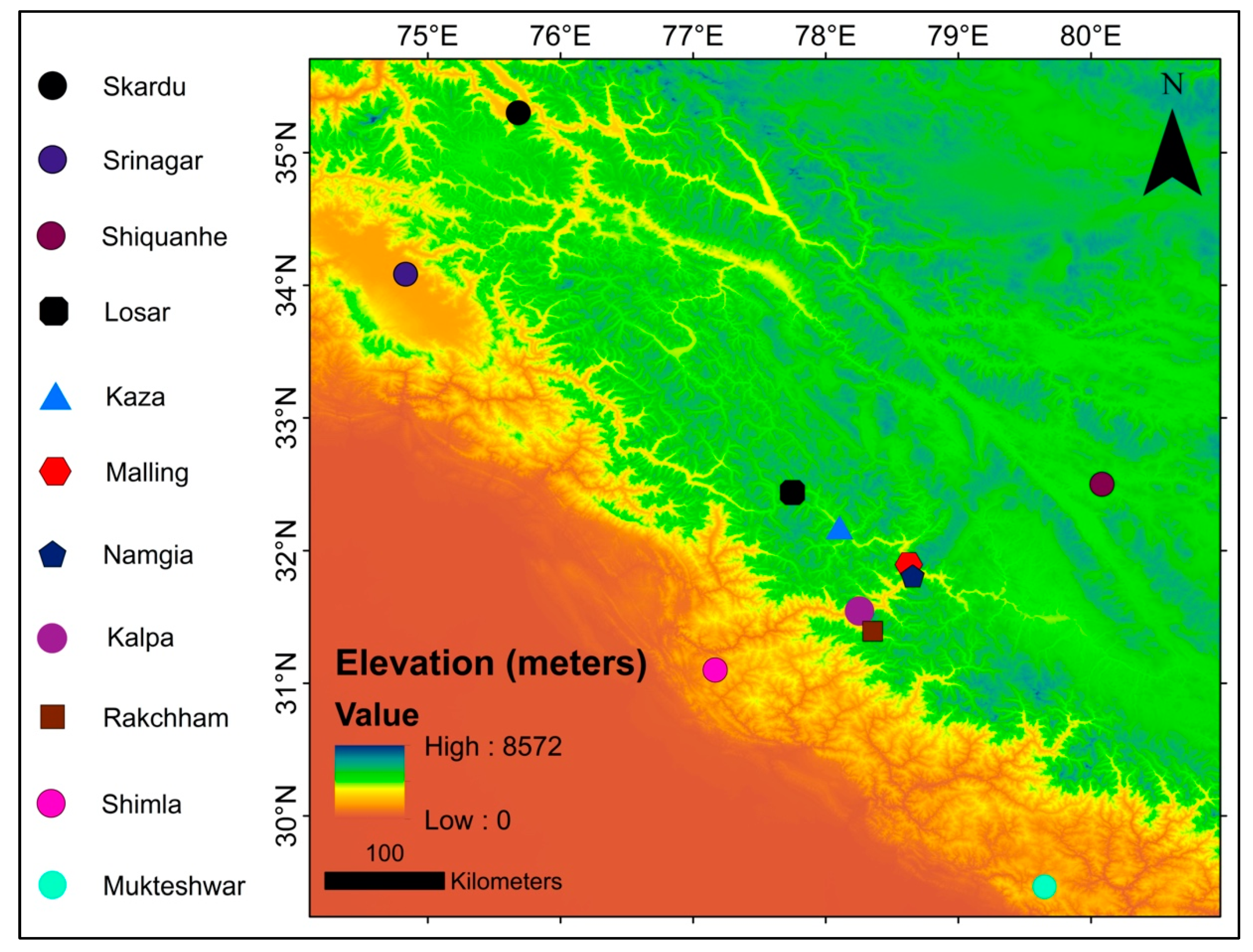
2. Study Area
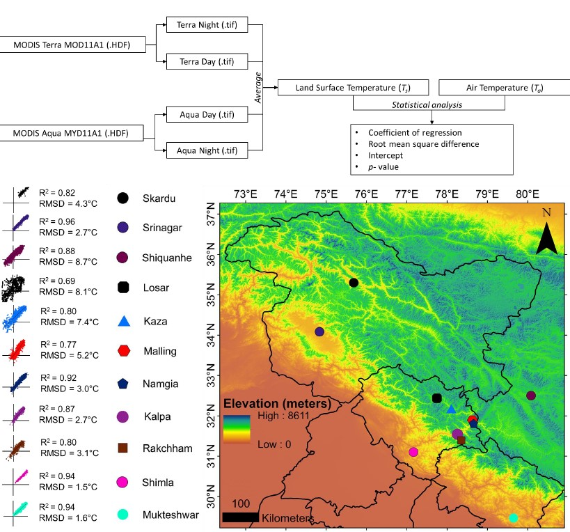
3. Materials and Methods
3.1. Air Temperature (Ta)
3.2. MODIS Data
3.3. Statistical Analyses
4. Results
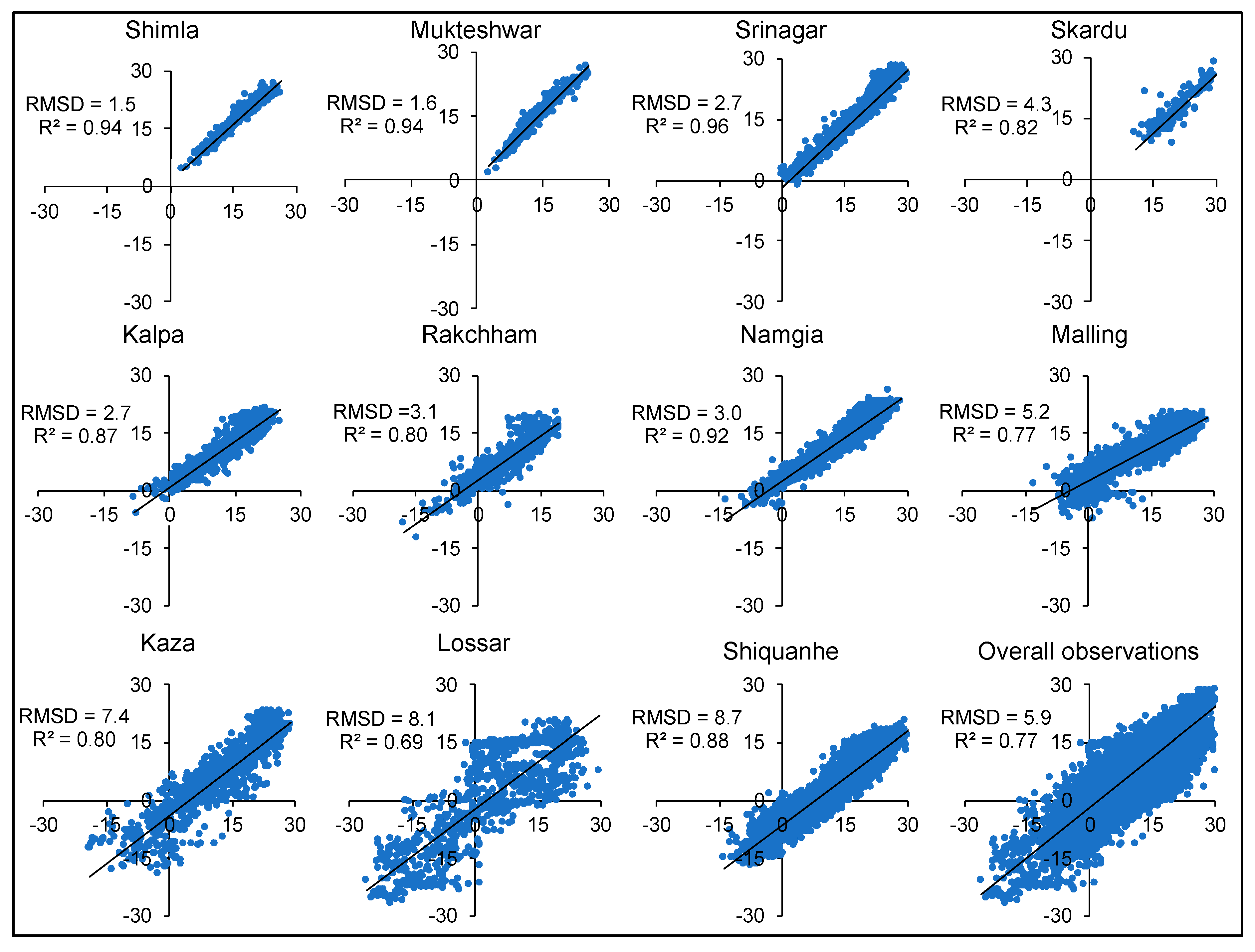
4.1. Ts vs. Ta Relationship
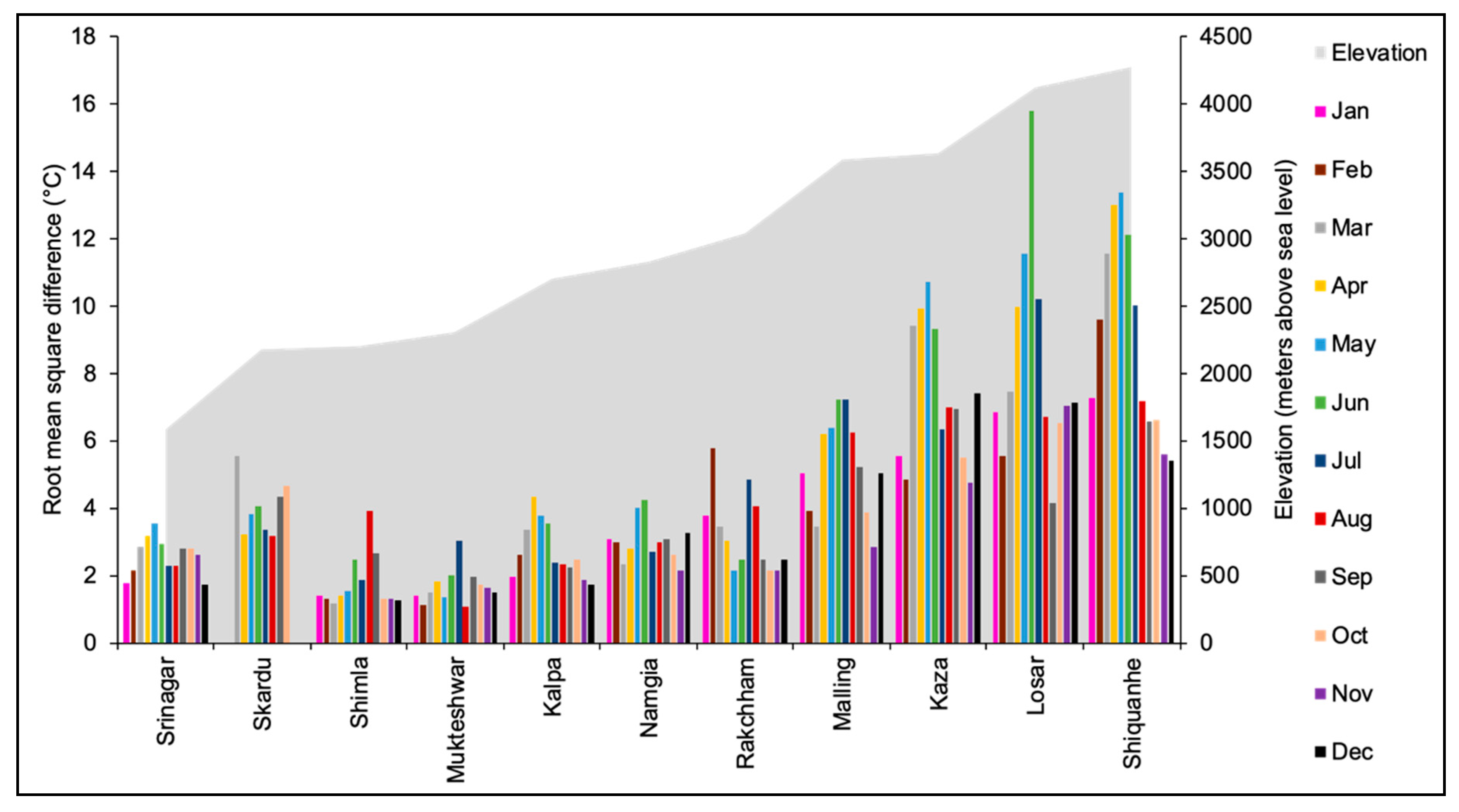
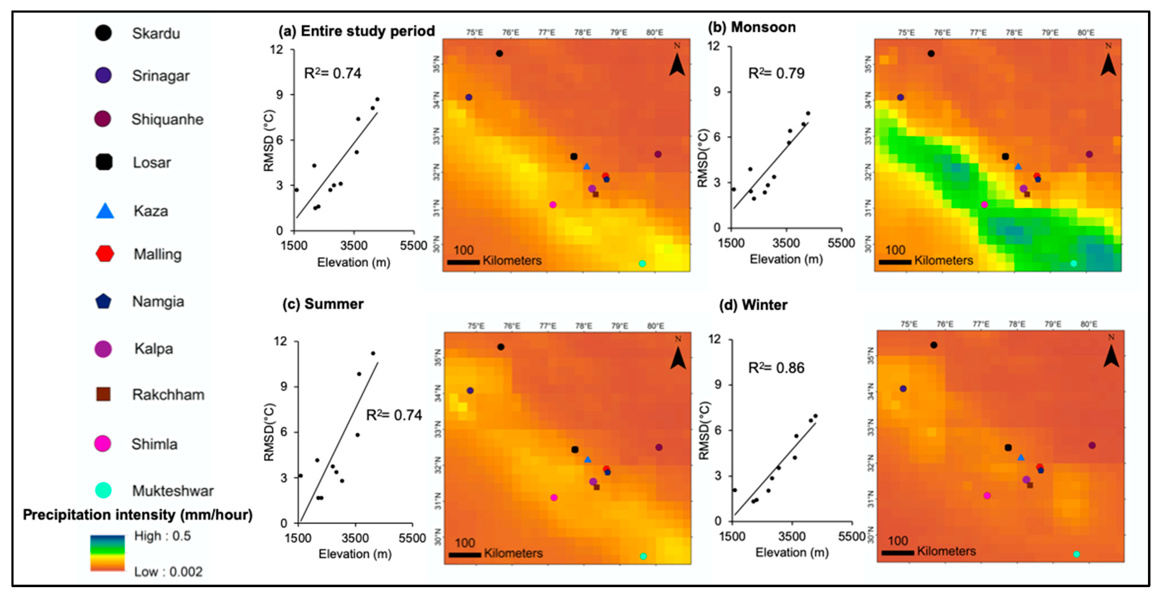
4.2. Altitudinal Relationship
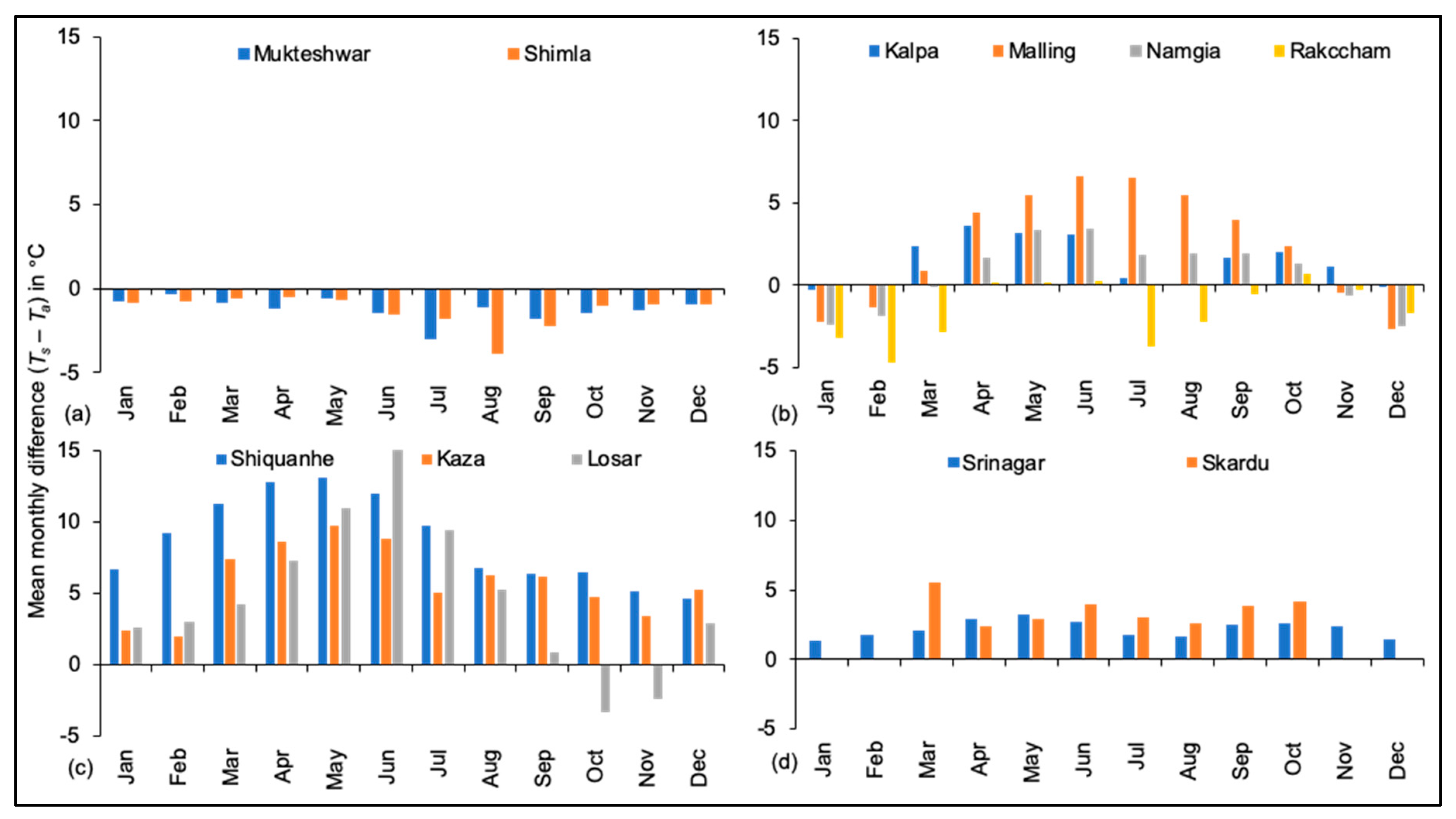
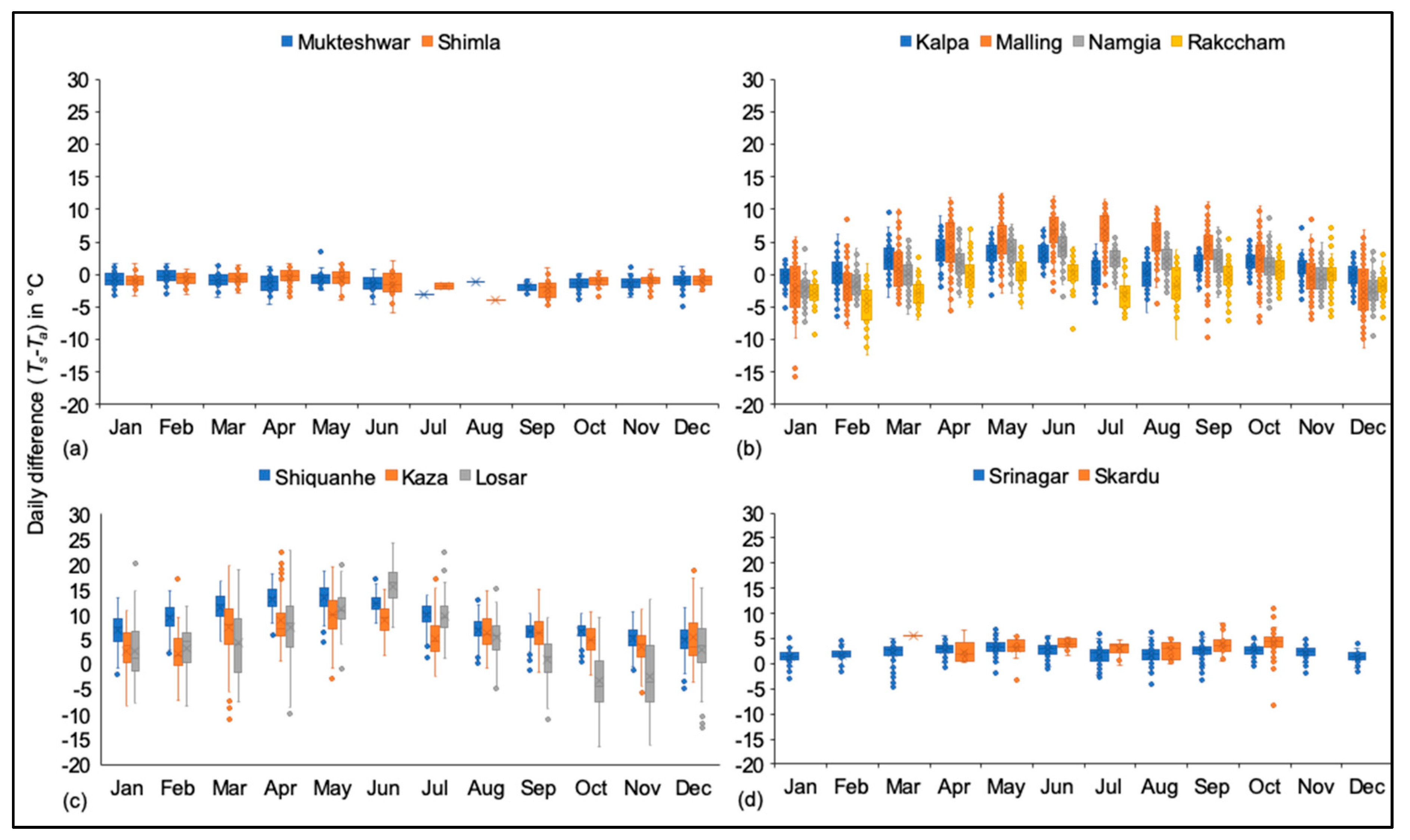
4.3. Seasonal Relationship
5. Discussion
6. Conclusions
Author Contributions
Funding
Acknowledgments
Conflicts of Interest
References
- Hansen, J.; Ruedy, R.; Sato, M.; Lo, K. Global surface temperature change. Rev. Geophys. 2010, 48, RG4004. [Google Scholar] [CrossRef] [Green Version]
- Jones, P.D. Hemispheric Surface Air Temperature Variations: A Reanalysis and an Update to 1993. J. Clim. 1994, 7, 1794–1802. [Google Scholar] [CrossRef]
- Hock, R. Temperature index melt modelling in mountain areas. J. Hydrol. 2003, 282, 104–115. [Google Scholar] [CrossRef]
- Kumar, R.; Singh, S.; Kumar, R.; Singh, A.; Bhardwaj, A.; Sam, L.; Randhawa, S.S.; Gupta, A. Development of a glacio-hydrological model for discharge and mass balance reconstruction. Water Resour. Manag. 2016, 30, 3475–3492. [Google Scholar] [CrossRef]
- Hatfield, J.L.; Prueger, J.H. Temperature extremes: Effect on plant growth and development. Weather Clim. Extrem. 2015, 10, 4–10. [Google Scholar] [CrossRef] [Green Version]
- Stoll, M.J.; Brazel, A.J. Surface-air temperature relationships in the urban environment of Phoenix, Arizona. Phys. Geogr. 1992, 13, 160–179. [Google Scholar] [CrossRef]
- Seiler, C.; Moene, A.F. Estimating Actual Evapotranspiration from Satellite and Meteorological Data in Central Bolivia. Earth Interact. 2011, 15, 1–24. [Google Scholar] [CrossRef]
- Screen, J.A.; Simmonds, I. The central role of diminishing sea ice in recent Arctic temperature amplification. Nature 2010, 464, 1334. [Google Scholar] [CrossRef] [Green Version]
- Ishida, T.; Kawashima, S. Use of cokriging to estimate surface air temperature from elevation. Theor. Appl. Climatol. 1993, 47, 147–157. [Google Scholar] [CrossRef]
- Snehmani; Bhardwaj, A.; Singh, M.K.; Gupta, R.D.; Joshi, P.K.; Ganju, A. Modelling the hypsometric seasonal snow cover using meteorological parameters. J. Spat. Sci. 2015, 60, 51–64. [Google Scholar] [CrossRef]
- Willmott, C.J.; Robeson, S.M. Climatologically aided interpolation (CAI) of terrestrial air temperature. Int. J. Climatol. 1995, 15, 221–229. [Google Scholar] [CrossRef]
- Bense, V.F.; Read, T.; Verhoef, A. Using distributed temperature sensing to monitor field scale dynamics of ground surface temperature and related substrate heat flux. Agric. For. Meteorol. 2016, 220, 207–215. [Google Scholar] [CrossRef] [Green Version]
- Sellers, P.J.; Dickinson, R.E.; Randall, D.A.; Betts, A.K.; Hall, F.G.; Berry, J.A.; Collatz, G.J.; Denning, A.S.; Mooney, H.A.; Nobre, C.A.; et al. Modeling the exchanges of energy, water, and carbon between continents and the atmosphere. Science 1997, 275, 502–509. [Google Scholar] [CrossRef] [PubMed] [Green Version]
- Luo, D.; Jina, H.; Marchenkoa, S.S.; Romanovsky, V.E. Difference between near-surface air, land surface and ground surface temperatures and their influences on the frozen ground on the Qinghai-Tibet Plateau. Geoderma 2018, 312, 74–85. [Google Scholar] [CrossRef]
- Hachem, S.; Allard, M.; Duguay, C. Using the MODIS land surface temperature product for mapping permafrost: An application to northern Québec and Labrador, Canada. Permafr. Periglac. Process. 2009, 20, 407–416. [Google Scholar] [CrossRef]
- Hachem, S.; Duguay, C.R.; Allard, M. Comparison of MODIS-derived land surface temperatures with ground surface and air temperature measurements in continuous permafrost terrain. Cryosphere 2012, 6, 51–69. [Google Scholar] [CrossRef] [Green Version]
- Ran, Y.; Li, X.; Jin, R.; Guo, J. Remote sensing of the mean annual surface temperature and surface frost number for mapping permafrost in China. Arct. Antarct. Alp. Res. 2015, 47, 255–265. [Google Scholar] [CrossRef] [Green Version]
- Benali, A.; Carvalho, A.C.; Nunes, J.P.; Carvalhais, N.; Santos, A. Estimating air surface temperature in Portugal using MODIS LST data. Remote Sens. Environ. 2012, 124, 108–121. [Google Scholar] [CrossRef]
- Mutiibwa, D.; Strachan, S.; Albright, T. Land Surface Temperature and Surface Air Temperature in Complex Terrain. IEEE J. Sel. Top. Appl. Earth Obs. Remote Sens. 2015, 8, 4762–4774. [Google Scholar] [CrossRef]
- Prihodko, L.; Goward, S.N. Estimation of air temperature from remotely sensed surface observations. Remote Sens. Environ. 1997, 60, 335–346. [Google Scholar] [CrossRef]
- Stisen, S.; Sandholt, I.; Nørgaard, A.; Fensholt, R.; Eklundh, L. Estimation of diurnal air temperature using MSG SEVIRI data in West Africa. Remote Sens. Environ. 2007, 110, 262–274. [Google Scholar] [CrossRef]
- Vancutsem, C.; Ceccato, P.; Dinku, T.; Connor, S.J. Evaluation of MODIS land surface temperature data to estimate air temperature in different ecosystems over Africa. Remote Sens. Environ. 2010, 114, 449–465. [Google Scholar] [CrossRef]
- Wan, Z.; Hook, S.; Hulley, G. MOD11A1 MODIS/Terra Land Surface Temperature/Emissivity Daily L3 Global 1km SIN Grid V006 [Data set]. NASA EOSDIS LP DAAC 2015. [Google Scholar] [CrossRef]
- Wan, Z.; Hook, S.; Hulley, G. MYD11A1 MODIS/Aqua Land Surface Temperature/Emissivity Daily L3 Global 1km SIN Grid V006 [Data set]. NASA EOSDIS LP DAAC 2015. [Google Scholar] [CrossRef]
- Shah, D.B.; Pandya, M.R.; Trivedi, H.J.; Jani, A.R. Estimating minimum and maximum air temperature using MODIS data over Indo-Gangetic Plain. J. Earth Syst. Sci. 2013, 122, 1593–1605. [Google Scholar] [CrossRef] [Green Version]
- Zhu, W.; Lű, A.; Jia, S. Estimation of daily maximum and minimum air temperature using MODIS land surface temperature products. Remote Sens. Environ. 2013, 130, 62–73. [Google Scholar] [CrossRef]
- Williamson, S.; Hik, D.; Gamon, J.; Kavanaugh, J.; Flowers, G. Estimating temperature fields from MODIS land surface temperature and air temperature observations in a sub-arctic alpine environment. Remote Sens. 2014, 6, 946–963. [Google Scholar] [CrossRef] [Green Version]
- Pepin, N.; Deng, H.; Zhang, H.; Zhang, F.; Kang, S.; Yao, T. An examination of temperature trends at high elevations across the Tibetan Plateau: The use of MODIS LST to understand patterns of elevation-dependent warming. J. Geophys. Res. Atmos. 2019, 124, 5738–5756. [Google Scholar] [CrossRef] [Green Version]
- Singh, S.; Kumar, R.; Bhardwaj, A.; Sam, L.; Shekhar, M.; Singh, A.; Kumar, R.; Gupta, A. The Indian Himalayan Region: A review of signatures of changing climate and vulnerability. WIREs Clim. Chang. 2016, 7, 393–410. [Google Scholar] [CrossRef] [Green Version]
- Immerzeel, W.W.; Van Beek, L.P.H.; Bierkens, M.F.P. Climate Change Will Affect the Asian Water Towers. Science 2010, 328, 1382–1385. [Google Scholar] [CrossRef]
- Sam, L.; Bhardwaj, A.; Kumar, R.; Buchroithner, M.F.; Martín-Torres, F.J. Heterogeneity in topographic control on velocities of Western Himalayan glaciers. Sci. Rep. 2018, 8, 12843. [Google Scholar] [CrossRef] [PubMed] [Green Version]
- Sam, L.; Bhardwaj, A.; Sinha, V.S.P.; Joshi, P.K.; Kumar, R. Use of Geospatial Tools to Prioritize Zones of Hydro-Energy Potential in Glaciated Himalayan Terrain. J. Indian Soc. Remote Sens. 2016, 44, 409–420. [Google Scholar] [CrossRef]
- Shekhar, M.; Bhardwaj, A.; Singh, S.; Ranhotra, P.S.; Bhattacharyya, A.; Pal, A.K.; Roy, I.; Martín-Torres, F.J.; María-Paz, Z. Himalayan glaciers experienced significant mass loss during later phases of little ice age. Sci. Rep. 2017, 7, 10305. [Google Scholar] [CrossRef] [PubMed]
- Bookhagen, B.; Burbank, D.W. Toward a complete Himalayan hydrological budget: Spatiotemporal distribution of snowmelt and rainfall and their impact on river discharge. J. Geophys. Res. 2010, 115. [Google Scholar] [CrossRef] [Green Version]
- National Centre for Environmental Information (NCEI). Available online: https://www.ncei.noaa.gov/ (accessed on 5 November 2019).
- Villarini, G.; Khouakhi, A.; Cunningham, E. On the impacts of computing daily temperatures as the average of the daily minimum and maximum temperatures. Atmos. Res. 2017, 198, 145–150. [Google Scholar] [CrossRef]
- Ma, Y.; Guttorp, P. Estimating daily mean temperature from synoptic climate observations. Int. J. Climatol. 2013, 33, 1264–1269. [Google Scholar] [CrossRef]
- NASA Earthdata Portal. Available online: https://earthdata.nasa.gov/ (accessed on 5 November 2019).
- Wan, Z. New refinements and validation of the MODIS land-surface temperature/emissivity products. Remote Sens. Environ. 2008, 112, 59–74. [Google Scholar] [CrossRef]
- Shah, H.L.; Zhou, T.; Huang, M.; Mishra, V. Strong influence of irrigation on water budget and land surface temperature in Indian sub-continental river basins. J. Geophys. Res. Atmos. 2019, 124, 1449–1462. [Google Scholar] [CrossRef]
- Goddard Earth Sciences Data and Information Services Center. TRMM (TMPA) Precipitation L3 1 Day 0.25 Degree × 0.25 Degree V7; Savtchenko, A., Ed.; GES DISC: Greenbelt, MD, USA, 2016. [Google Scholar] [CrossRef]
- Williamson, S.N.; Hik, D.S.; Gamon, J.A.; Jarosch, A.H.; Anslow, F.S.; Clarke, G.K.; Rupp, T.S. Spring and summer monthly MODIS LST is inherently biased compared to air temperature in snow covered sub-Arctic mountains. Remote Sens. Environ. 2017, 189, 14–24. [Google Scholar] [CrossRef]
- Immerzeel, W.W.; Petersen, L.; Ragettli, S.; Pellicciotti, F. The importance of observed gradients of air temperature and precipitation for modeling runoff from a glacierized watershed in the Nepalese Himalayas. Water Resour. Res. 2014, 50, 2212–2226. [Google Scholar] [CrossRef] [Green Version]
- Singh, S.; Kumar, R.; Bhardwaj, A.; Kumar, R.; Singh, A. Changing climate and glacio-hydrology: A case study of Shaune Garang basin, Himachal Pradesh. Int. J. Hydrol. Sci. Technol. 2018, 8, 258–272. [Google Scholar] [CrossRef]
- Singh, P.; Haritashya, U.K.; Kumar, N. Modelling and estimation of different components of streamflow for Gangotri Glacier basin, Himalayas. Hydrol. Sci. J. 2008, 53, 309–322. [Google Scholar] [CrossRef]
- Wulf, H.; Bookhagen, B.; Scherler, D. Differentiating between rain, snow, and glacier contributions to river discharge in the western Himalaya using remote-sensing data and distributed hydrological modeling. Adv. Water Resour. 2016, 88, 152–169. [Google Scholar] [CrossRef] [Green Version]
- Kraaijenbrink, P.D.A.; Bierkens, M.F.P.; Lutz, A.F.; Immerzeel, W.W. Impact of a global temperature rise of 1.5 degrees Celsius on Asia’s glaciers. Nature 2017, 549, 257–260. [Google Scholar] [CrossRef]
- Shekhar, M.S.; Chand, H.; Kumar, S.; Srinivasan, K.; Ganju, A. Climate-change studies in the western Himalaya. Ann. Glaciol. 2010, 51, 105–112. [Google Scholar] [CrossRef] [Green Version]
- Liang, E.; Dawadi, B.; Pederson, N.; Eckstein, D. Is the growth of birch at the upper timberline in the Himalayas limited by moisture or by temperature? Ecology 2014, 95, 2453–2465. [Google Scholar] [CrossRef] [Green Version]
- Xu, J.; Grumbine, R.E.; Shrestha, A.; Eriksson, M.; Yang, X.; Wang, Y.; Wilkes, A. The Melting Himalaya: Cascading Effects of Climate Change on Water, Biodiversity, and Livelihoods. Conserv. Biol. 2009, 23, 520–530. [Google Scholar] [CrossRef]
- Archer, D.R.; Forsythe, N.; Fowler, H.J.; Shah, S.M. Sustainability of water resources management in the Indus Basin under changing climatic and socio economic conditions. Hydrol. Earth Syst. Sci. 2010, 14, 1669–1680. [Google Scholar] [CrossRef] [Green Version]
- Malla, G. Climate Change and Its Impact on Nepalese Agriculture. J. Agric. Environ. 2009, 9, 62–71. [Google Scholar] [CrossRef] [Green Version]
- Kimball, J.S.; Running, S.W.; Nemani, R. An improved method for estimating surface humidity from daily minimum temperature. Agric. For. Meteorol. 1997, 85, 87–98. [Google Scholar] [CrossRef]
- Good, E.J. An in situ-based analysis of the relationship between land surface “skin” and screen-level air temperatures. J. Geophys. Res. Atmos. 2016, 121, 8801–8819. [Google Scholar] [CrossRef]
- Good, E.J.; Ghent, D.J.; Bulgin, C.E.; Remedios, J.J. A spatiotemporal analysis of the relationship between near-surface air temperature and satellite land surface temperatures using 17 years of data from the ATSR series. J. Geophys. Res. Atmos. 2017, 122, 9185–9210. [Google Scholar] [CrossRef]
- Kulkarni, A.V.; Rathore, B.P.; Singh, S.K. Distribution of seasonal snow cover in central and western Himalaya. Ann. Glaciol. 2010, 51, 123–128. [Google Scholar] [CrossRef] [Green Version]
- Bhardwaj, A.; Singh, S.; Sam, L.; Bhardwaj, A.; Martin-Torres, F.J.; Singh, A.; Kumar, R. MODIS-based estimates of strong snow surface temperature anomaly related to high altitude earthquakes of 2015. Remote Sens. Environ. 2017, 188, 1–8. [Google Scholar] [CrossRef]
- Niclos, R.; Valiente, J.A.; Barberà, M.J.; Caselles, V. Land surface air temperature retrieval from EOS-MODIS images. IEEE Geosci. Remote Sens. Lett. 2013, 11, 1380–1384. [Google Scholar] [CrossRef] [Green Version]


| Sl. No. | Name of the Station | Elevation (m) | Period | Organization | Precipitation Regime |
|---|---|---|---|---|---|
| 1. | Kalpa | 2707 | 07-Jul-02–31-Dec-09 | IMD | Transition |
| 2. | Kaza | 3631 | 07-Jul-02–31-Dec-09 | IMD | Shadow |
| 3. | Namgia | 2832 | 07-Jul-02–31-Dec-09 | BBMB | Transition |
| 4. | Rakchham | 3046 | 07-Jul-02–31-Dec-09 | BBMB | Transition |
| 5. | Malling | 3588 | 07-Jul-02–31-Dec-09 | BBMB | Transition |
| 6. | Losar | 4122 | 07-Jul-02–31-Dec-09 | BBMB | Shadow |
| 7. | Mukteshwar | 2311 | 13-Dec-15–30-Sept-19 | GHCN | Monsoon |
| 8. | Shimla | 2202 | 01-Jan-16–30-Sept-19 | GHCN | Monsoon |
| 9. | Shiquanhe | 4280 | 06-Jul-02–30-Sept-19 | GHCN | Shadow |
| 10. | Skardu | 2181 | 02-Oct-02–30-Sept-19 | GHCN | Shadow |
| 11. | Srinagar | 1587 | 05-Jul-02–30-Sept-19 | GHCN | Shadow |
| Sl. No. | Data Characteristics | Terra | Aqua | ||
|---|---|---|---|---|---|
| MOD11A1 | MOD11A2 | MYD11A1 | MYD11A2 | ||
| 1. | Temporal resolution | Daily | 8-day | Daily | 8-day |
| 2. | Spatial resolution | 1 km | 1 km | ||
| 3. | Available from | February, 2000 | July, 2002 | ||
| 4. | Local day time of observation | 10:30–11:30 | 12:30–13:30 | ||
| 5. | Local night time of observation | 21:30–22:30 | 00:30–01:30 | ||
| Name of the Station | Observations | R2 | SE | RMSD | Regression Equation | |||||
|---|---|---|---|---|---|---|---|---|---|---|
| Daily | 8-day | Daily | 8-day | Daily | 8-day | Daily | 8-day | Daily | 8-day | |
| Srinagar | 1771 | 664 | 0.96 | 0.97 | 1.38 | 1.23 | 2.7 | 2.5 | Ta = 0.96Ts − 1.64 | Ta = 0.92Ts − 0.72 |
| Skardu | 193 | 35 | 0.82 | 0.93 | 2.06 | 1.22 | 4.3 | 3.2 | Ta = 0.94Ts − 2.67 | Ta = 0.82Ts − 0.71 |
| Shimla | 304 | 55 | 0.94 | 0.97 | 1.22 | 0.96 | 1.5 | 1.4 | Ta = 0.97Ts + 1.43 | Ta = 0.94Ts + 1.78 |
| Mukteshwar | 355 | 63 | 0.94 | 0.96 | 1.16 | 1.05 | 1.6 | 1.2 | Ta = 1.03Ts + 0.62 | Ta = 0.99Ts + 0.76 |
| Kalpa | 866 | 337 | 0.87 | 0.89 | 1.93 | 1.95 | 2.7 | 2.5 | Ta = 0.80Ts + 0.93 | Ta = 0.83Ts + 0.98 |
| Namgia | 1141 | 338 | 0.92 | 0.95 | 1.96 | 1.78 | 3.0 | 2.6 | Ta = 0.75Ts + 2.39 | Ta = 0.79Ts + 2.14 |
| Rakchham | 820 | 310 | 0.79 | 0.88 | 2.45 | 2.09 | 3.1 | 2.9 | Ta = 0.77Ts + 2.63 | Ta = 0.79Ts + 2.71 |
| Malling | 1093 | 332 | 0.77 | 0.85 | 2.83 | 2.51 | 5.2 | 4.5 | Ta = 0.59Ts + 2.51 | Ta = 0.64Ts + 2.30 |
| Kaza | 1028 | 333 | 0.80 | 0.83 | 4.29 | 4.37 | 7.4 | 7.2 | Ta = 0.83Ts − 3.92 | Ta = 0.86Ts − 4.17 |
| Losar | 1019 | 308 | 0.69 | 0.77 | 7.12 | 6.59 | 8.1 | 7.8 | Ta = 0.81Ts − 2.16 | Ta = 0.84Ts − 3.23 |
| Shiquanhe | 2511 | 777 | 0.88 | 0.97 | 3.19 | 1.56 | 8.7 | 8.9 | Ta = 0.82Ts − 6.43 | Ta = 0.80Ts − 6.46 |
| Monsoon-Dominated | 659 | 118 | 0.94 | 0.96 | 1.19 | 1.02 | 1.5 | 1.3 | Ta = 1.00Ts + 1.01 | Ta = 0.96Ts + 1.31 |
| Transition | 3920 | 1317 | 0.82 | 0.88 | 2.56 | 2.31 | 3.7 | 3.2 | Ta = 0.69Ts + 2.45 | Ta = 0.74Ts + 2.27 |
| Westerlies-Dominated | 1964 | 699 | 0.95 | 0.97 | 1.51 | 1.24 | 2.9 | 2.5 | Ta = 0.95Ts − 1.61 | Ta = 0.91Ts − 0.69 |
| Precipitation Shadow | 4558 | 1418 | 0.77 | 0.85 | 4.92 | 4.22 | 8.4 | 8.4 | Ta = 0.80Ts − 4.70 | Ta = 0.80Ts − 5.06 |
| Overall Observations | 11,101 | 3552 | 0.77 | 0.80 | 4.76 | 4.49 | 5.9 | 5.7 | Ta = 0.87Ts − 1.83 | Ta = 0.85Ts − 1.63 |
© 2019 by the authors. Licensee MDPI, Basel, Switzerland. This article is an open access article distributed under the terms and conditions of the Creative Commons Attribution (CC BY) license (http://creativecommons.org/licenses/by/4.0/).
Share and Cite
Singh, S.; Bhardwaj, A.; Singh, A.; Sam, L.; Shekhar, M.; Martín-Torres, F.J.; Zorzano, M.-P. Quantifying the Congruence between Air and Land Surface Temperatures for Various Climatic and Elevation Zones of Western Himalaya. Remote Sens. 2019, 11, 2889. https://0-doi-org.brum.beds.ac.uk/10.3390/rs11242889
Singh S, Bhardwaj A, Singh A, Sam L, Shekhar M, Martín-Torres FJ, Zorzano M-P. Quantifying the Congruence between Air and Land Surface Temperatures for Various Climatic and Elevation Zones of Western Himalaya. Remote Sensing. 2019; 11(24):2889. https://0-doi-org.brum.beds.ac.uk/10.3390/rs11242889
Chicago/Turabian StyleSingh, Shaktiman, Anshuman Bhardwaj, Atar Singh, Lydia Sam, Mayank Shekhar, F. Javier Martín-Torres, and María-Paz Zorzano. 2019. "Quantifying the Congruence between Air and Land Surface Temperatures for Various Climatic and Elevation Zones of Western Himalaya" Remote Sensing 11, no. 24: 2889. https://0-doi-org.brum.beds.ac.uk/10.3390/rs11242889