Features of the Cloud Base Height and Determining the Threshold of Relative Humidity over Southeast China

Key Laboratory for Semi-Arid Climate Change of the Ministry of Education, College of Atmospheric Sciences, Lanzhou University, Lanzhou 730000, China
*
Author to whom correspondence should be addressed.
Remote Sens. 2019, 11(24), 2900; https://0-doi-org.brum.beds.ac.uk/10.3390/rs11242900
Submission received: 13 October 2019
/
Revised: 14 November 2019
/
Accepted: 3 December 2019
/
Published: 5 December 2019
(This article belongs to the Special Issue High Resolution Active Optical Remote Sensing Observations of Aerosols, Clouds and Aerosol-Cloud Interactions and Their Implication to Climate)
Abstract
:Clouds play a critical role in adjusting the global radiation budget and hydrological cycle; however, obtaining accurate information on the cloud base height (CBH) is still challenging. In this study, based on Lidar and aircraft soundings, we investigated the features of the CBH and determined the thresholds of the environmental relative humidity (RH) corresponding to the observed CBHs over Southeast China from October 2017 to September 2018. During the observational period, the CBHs detected by Lidar/aircraft were commonly higher in cold months and lower in warm months; in the latter, 75.91% of the CBHs were below 2000 m. Overall, the RHs at the cloud base were mainly distributed between 70 and 90% for the clouds lower than 1000 m, in which the most concentrated RH was approximately 80%. In addition, for the clouds with a cloud base higher than 1000 m, the RH thresholds decreased dramatically with increasing CBH, where the RH thresholds at cloud bases higher than 2000 m could be lower than 60%. On average, the RH thresholds for determining the CBHs were the highest (72.39%) and lowest (63.56%) in the summer and winter, respectively, over Southeast China. Therefore, to determine the CBH, a specific threshold of RH is needed. Although the time period covered by the collected CBH data from Lidar/aircraft is short, the above analyses can provide some verification and evidence for using the RH threshold to determine the CBH.

1. Introduction
Clouds can adjust the Earth’s energy budget and hydrological cycle through dynamic and thermal processes [1,2,3] and further drive the climate to change globally [4]. However, considerable uncertainties in cloud properties have been found [5], further contributing to errors in weather forecasting and climate prediction [6]. The immense uncertainties regarding clouds include optical [7,8,9], microphysical [10,11], and geometrical [12,13] features, the effects on the radiation budget [14], interactions with aerosols [15,16,17,18,19,20,21], and impacts on precipitation [22,23]. In particular, the cloud profile is poorly understood at present and remains a primary source of uncertainty in global weather and climate research [24].
The cloud base height (CBH), which is an important parameter of the cloud vertical profile, largely determines the energy exchanges between the clouds and surface. Accordingly, determining the CBHs is extremely critical for weather forecasting and ensuring flight safety [25,26]. Currently, retrieving the CBH generally relies primarily on satellite and ground-based observations. Space-borne active satellite remote sensing (e.g., the cloud profile radar (CPR) mounted on CloudSat and the Cloud-Aerosol Lidar with Orthogonal Polarization (CALIOP) aboard Cloud-Aerosol Lidar and Infrared Satellite Observation (CALIPSO)) has allowed cloud profile information to be obtained globally [27,28,29]. Some studies have estimated the CBH by applying both satellite-derived cloud optical depth, cloud water path, and some additional parameterizations that connect cloud optical depth with cloud geometrical thickness [30,31]. Other methods have also been used to estimate the CBH [32,33,34]. For example, Liang et al. [35] estimated the CBH by combining measurements from CloudSat/CALIPSO and Moderate-resolution Imaging Spectroradiometer (MODIS) based on the International Satellite Cloud Climatology Project (ISCCP) cloud-type classification and a weighted algorithm; unfortunately, the calculation of the CBH is dependent on an assumption of the cloud water content [36]. However, a comparison with the ground-based active remote sensing of clouds revealed large uncertainties in the CBH from satellite observations [37]. Therefore, obtaining information on the CBH with high accuracy is urgent.
Compared with satellite observations, ground-based cloud observations can provide CBH measurements with higher accuracy [34]. Some retrievals of the CBH are based on Lidar instruments [33], ceilometers [38], radiosondes [39,40,41,42], and total-sky-imager (TSI) [43]. Long-term research on the CBH measurements by radiosondes and ceilometer has been ongoing such as an analysis of 25-year CBHs measured by ceilometer at the Arctic site [44]. Some inter-comparisons among ground-based instruments have been performed [45,46,47,48,49]. In addition, some methods for calculating the CBHs have been reported by some earlier studies. Chernykh and Eskridge [50] proposed a method for judging the position of clouds using the second derivative of temperature and relative humidity (RH) versus the height in the ground-based soundings. For a long time, good agreement between the CBH and the lifting condensation level (LCL) estimated from the surface layer air have been confirmed and applied [51,52,53]. On this basis, Romps [54] gave the dependence of LCL on the temperature and RH and the conditions for cloud formation at heights such as the lifting deposition level (LDL) and the lifting freezing level (LFL). Wang and Rossow [2] postulated that an RH threshold value of 84% could be used to determine the cloud base location based on rawinsonde data. Additionally, Zhang et al. [42] performed an uncertainty analysis on the sensitivity of the CBH to different RH thresholds (83%, 84%, and 85%). To some degree, RH information at the cloud layer is significant in determining the CBHs from ground-based observations. Thus, an assessment of the RH threshold that can best determine the CBH is needed.
In this study, based on Lidar, pilot balloon, and aircraft soundings, the features of the CBH and the threshold of the environmental RH to determine the cloud base over Southeast China were investigated in detail. First, a comparison among the CBHs derived from three kinds of ground-based observations was performed. The observations with high accuracy were then selected as the reference. Next, combining the RH profiles from ERA-Interim data, the RH thresholds were calculated corresponding to the observed CBHs. Finally, the RH thresholds in different seasons for different CBHs were analyzed.
2. Datasets and Methods
2.1. Ground-Based Observations
At numerous sites throughout Southeast China (blue triangles in Figure 1), we performed observations with cloud Lidar (laser ceilometer), pilot balloon, and aircraft soundings from October 2017 to September 2018. The information on the sites is listed in Table 1.
We derived the cloud height using a cloud Lidar, whose emission source was a InGaAs 905 nm wavelength and 1.76 μJ pulse energy with a pulse repetition frequency of 1000 Hz. The pulse duration was 45 ns, and the beam divergence was less than 3 mrad. The detection range of cloud Lidar spans from 20 m to 7600 m with a vertical resolution of 3.8 m and a temporal resolution of 30 seconds. Lidar can scan the atmosphere with an elevation angle ranging from −30° to 30° and an azimuth in the range of 0–240°. The details about the technical specifications of the cloud Lidar used in this study are shown in Table 2. The retrieved CBH data [55,56] at seven sites from October 2017 to September 2018 were used.
Meanwhile, the CBH observations sounded by aircraft were also used in this study. The CBH detected by the aircraft soundings is obtained when the aircraft is flying upward through the cloud at the observational sites. When the aircraft enters the cloud, the pilot gives an altitude report for that moment, which is considered the height of the cloud base.
Additionally, a pilot balloon together with a GYR1 electronic optical wind theodolite was used to detect the CBH. After releasing a pilot balloon with a fixed rise velocity (ω) from the surface, a theodolite telescope is used to track the balloon. When the balloon starts to enter the clouds, the angular coordinate (elevation angle and azimuth angle) can be recorded. Then, the duration from the time of releasing balloon to the time of entering the cloud (t) can be calculated. Finally, the CBH can be estimated as the product of ω and , that is, .
2.2. Clouds and the Earth’s Radiant Energy System (CERES)
Cloud fraction and cloud base pressure data (SYN dataset) from October 2017 to September 2018 derived from Clouds and the Earth’s Radiant Energy System (CERES) mounted on the Aqua satellite were used in this paper. The temporal and spatial resolutions of these CERES data are hourly and 1° × 1°, respectively [57]. Here, the cloud base pressure (CBP) data provided by CERES were used for an intercomparison with the above-mentioned ground-based observations. According to the locations of the ground-based sites and observational time, the CBPs from the CERES data corresponding to the site location were extracted for a comparison with the calculated CBPs from CBHs.
2.3. ERA-Interim Reanalysis Data
ERA-Interim data released by the European Centre for Medium-Range Weather Forecasts (ECMWF) can provide assimilated reanalysis data four times a day (the temporal resolution is 6 h). In this study, RH profiles with a horizontal spatial resolution of 0.25° × 0.25° were used. In the vertical direction, the RH profiles had 37 layers from 1000 hPa to 1 hPa. The RHs employed in this study were extracted from the ERA-Interim data at 20 levels (from 1000 to 300 hPa) with a temporal resolution of 6 hours (0:00, 6:00, 12:00, and 18:00 UTC) [58].
2.4. Method of Conversion from Cloud Base Height (CBH) to Cloud Base Pressure (CBP)
In the cloud base datasets, the cloud base information from the CERES data is scaled by pressure (unit: hPa), while the CBHs detected by cloud Lidar and aircraft are measured as the geometric height (unit: m). To compare the ground-based measurement, a conversion from the CBH to the CBP is needed. Here, according to the pressure-height formula of polytropic atmosphere [59], CBP can be calculated from CBH.
where is the acceleration of gravity, here, it takes as 9.8 m/s; is the gas constant, ; and is the temperature lapse rate, taken as 6.5 K/km here. is the atmospheric pressure at the surface. Based on Equation (2), the virtual air temperature at 2 m () can be calculated from specific humidity () based on ERA-Interim data and observed temperature at the ground-based sites. The virtual air temperature at the cloud base () can be further calculated by Equation (3). Finally, based on the above formulas, the CBP can be calculated.
Based on the RH profiles from the ERA reanalysis data, the RH values at the cloud base can be extracted according to the CBPs calculated according to the above method, and the extracted RH value is regarded as the RH threshold at the cloud base.
3. Results
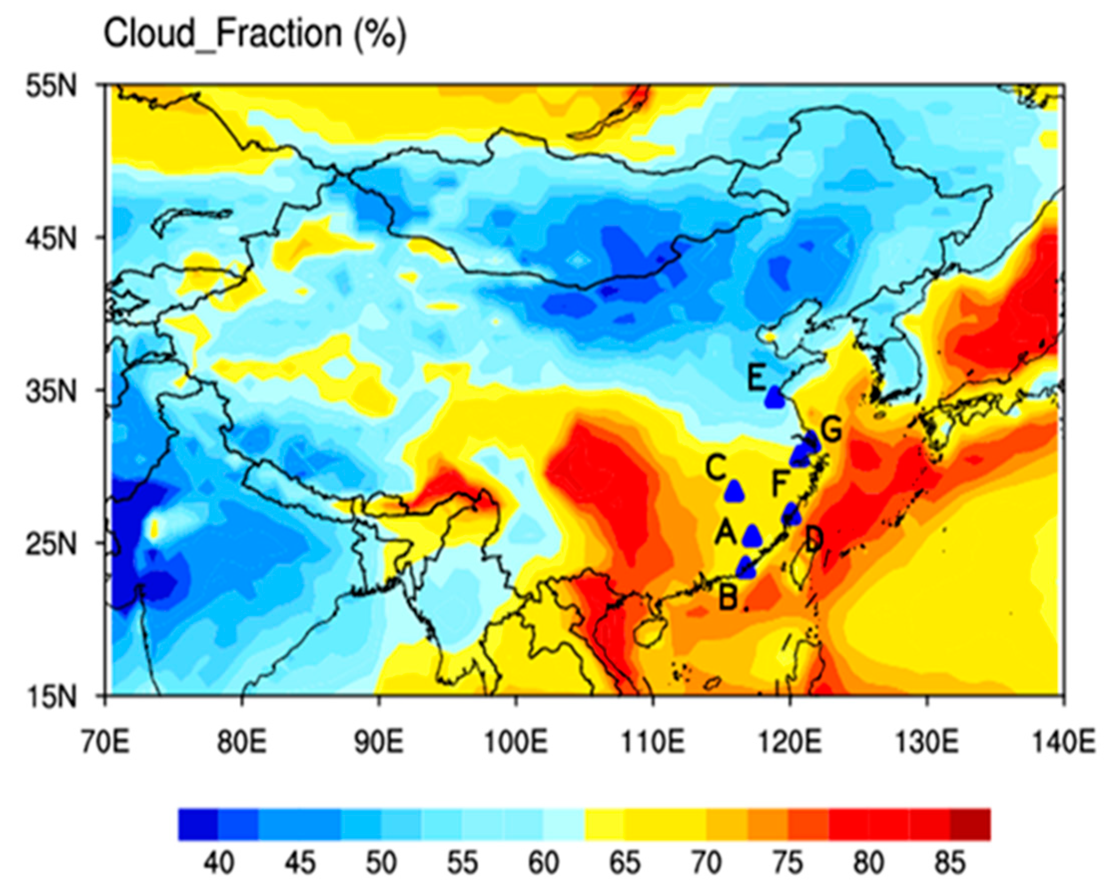
Figure 1 shows the distribution of observational sites (blue triangles) and the annual mean cloud fraction derived from CERES product in China from October 2017 to September 2018. As shown in Figure 1, during the above period, a high cloud fraction was distributed across South China with a value of approximately 80%. Low-value areas were located in North China, especially Inner Mongolia, with a minimum cloud fraction of 37.35%. Among the seven sites (blue triangles in Figure 1) involved in this study, the annual mean cloud fractions over sites C and D were approximately 70%, while those over sites A, B, and F were approximately 65%; however, the lowest cloud fraction (below 60%) was found over site E.
3.1. Intercomparison among the CBHs from Multi-Sourced Data
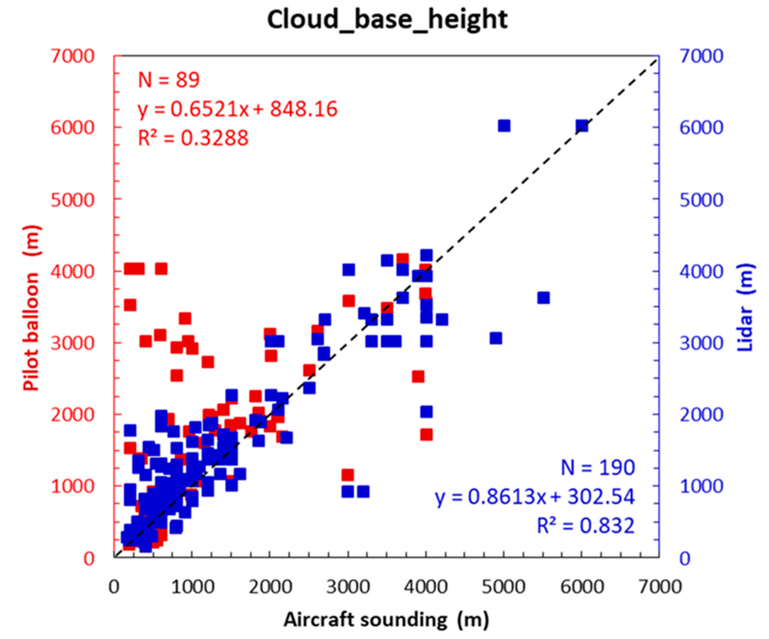
Compared with satellite measurements, ground-based cloud observations can provide CBH measurements with higher accuracy and a continuous temporal coverage. Moreover, aircraft soundings can provide more accurate CBH information than ground-based observations. Therefore, aircraft-sounded CBHs were considered to be an accurate reference in this study. In the subsequent analyses, the CBHs derived from two kinds of ground-based observations, pilot balloon and cloud Lidar, and from aircraft soundings during the period from October 2017 to September 2018 were analyzed at each of the seven sites (details as shown in Figure 1 and Table 1) to give the features of the CBH over those areas. Figure 2 shows a comparison of the CBHs sounded by aircraft with those detected by cloud Lidar and pilot balloon during the observational period. The results show that the correlation coefficient between the aircraft-sounded and Lidar-observed CBH was 0.86, which indicates good consistency between the CBHs detected by the cloud Lidar and those sounded by the aircraft. In addition, most of the CBHs detected by the Lidar were somewhat higher than those sounded by aircraft when the cloud bases were lower than 2000 m. However, when the cloud bases were higher than 2000 m, most of the Lidar-observed CBHs were slightly lower than the aircraft-soundings. Additionally, comparing the results detected by the pilot balloon with the CBHs sounded by aircraft, most of the CBHs sounded by the former were significantly higher than those sounded by the latter; the correlation coefficient was 0.65. Thus, the CBH data detected by both Lidar and aircraft were regarded as accurate values. In the following analyses, these two sets of data were complementary and used in conjunction to analyze the features of the CBH over Southeast China.
3.2. Features of the CBH over Southeast China
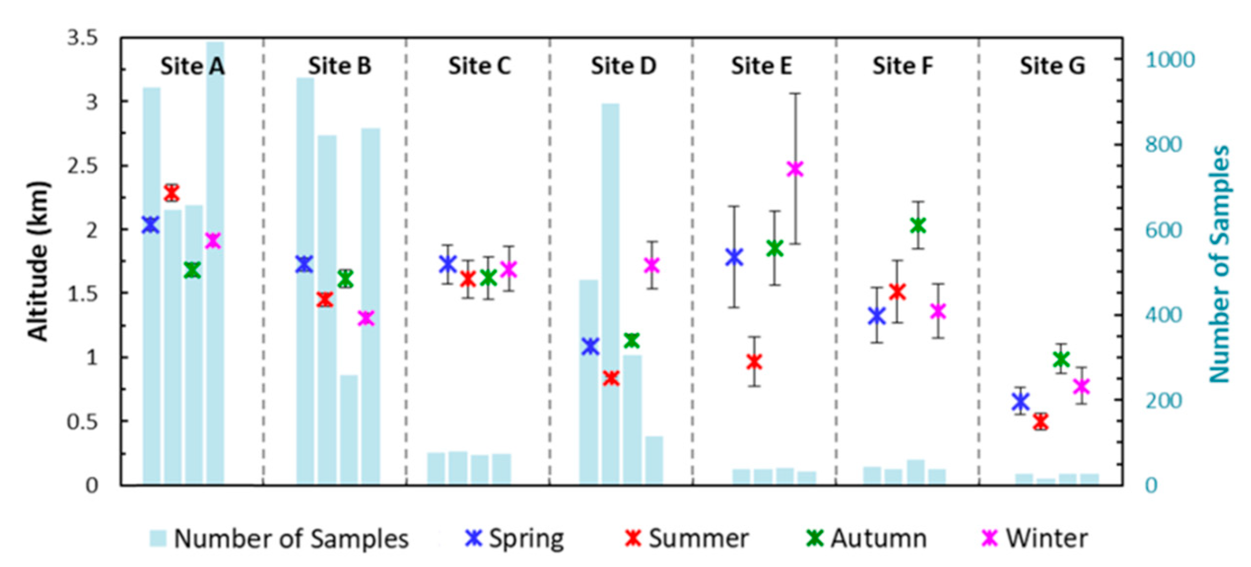
Based on the CBH samples detected by the cloud Lidar and aircraft, the seasonal variations of the CBH during the period from October 2017 to September 2018 at seven sites were analyzed, as shown in Figure 3, 75.91% of the CBH values at the seven sites were primarily below 2000 m. Overall, the CBHs in the summer were consistently lower than those in the other seasons at most of the sites except for site A. In addition, the summer CBHs were below 1000 m at sites D, E, and G, which are located along the oceanic coast. In this sense, at site C, which is farther from the ocean than the other sites, the seasonal variation of the CBH is relatively small throughout the whole year. Therefore, at sites near the ocean, monsoon systems could affect the CBH, which may be the reason for the seasonal CBH discrepancies among the different sites. Here, the error bars reflect the standard errors based on the means of the CBH samples at the seven sites. The standard errors at the sites are small, except for sites E and F, which indicates the reliability of the statistical results with large sample sizes.
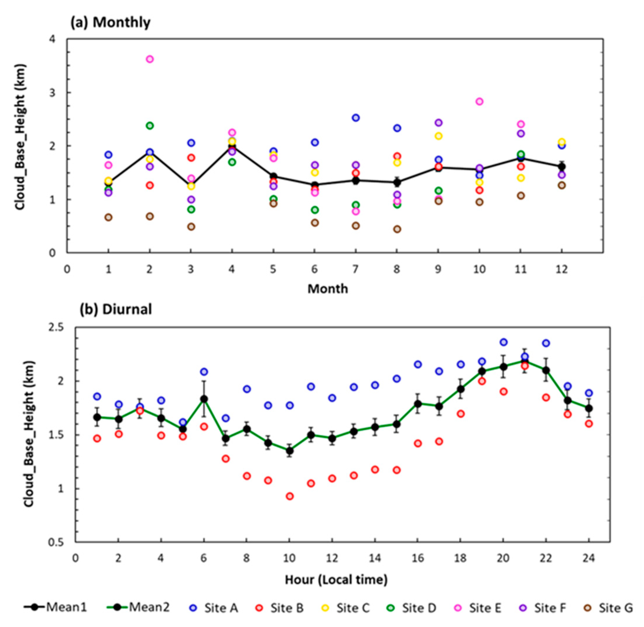
Furthermore, the monthly and diurnal variations of the CBH were similarly analyzed, as illustrated in Figure 4. Due to the absence of records at some sites where observations are performed only at certain times of day, fewer sites provided diurnal variation information (Figure 4b) than sites that provide monthly variation information (Figure 4a). Relative to the average CBHs at all sites (black line in Figure 4a), the lower CBHs were found in June–August, while the higher CBHs occur in February and April. Overall, most of the CBHs (75.91%) observed at seven sites were below 2000 m; in addition, the higher CBHs appeared in cold months, while the lower ones occurred in warmer months. Specifically, as shown in Figure 4a, the average CBHs over site A in most months (January, March, and May–August) were higher values relatively, which was also reflected by the diurnal variation of the CBH (Figure 4b). Meanwhile, for the whole year, the monthly mean CBHs over site G presented the lowest values (below 1000 m) among the seven sites, which is in agreement with the seasonal mean results in Figure 3. As shown in Figure 4b, overall, the mean values of the CBHs at sites A and B (green line in Figure 4b) were lower in the daytime than the nocturnal ones. Moreover, it was found that the CBHs over site B were much lower than those at site A, especially in the daytime (from 06:00 to 18:00). This phenomenon may be related to the fact that site B is located closer to the ocean than site A (as shown in Figure 1), as the abundance of water vapor from the ocean is beneficial to the formation of water clouds over site B.
3.3. Features of the Relative Humidity (RH) Threshold for Determining the CBH over Southeast China
According to Wang et al. [2], the CBH can be determined by the RH, and an RH of 84% was used as a threshold to determine the cloud base location. However, the scarcity of the sounding data limited an in-depth verification of determining the CBH by an RH threshold. Based on the above CBH data detected by cloud Lidar and aircraft, features of the RH thresholds used to determine the CBHs over these observational sites were investigated in the following analysis. The RH profiles derived from ERA reanalysis data together with observed surface air temperature and pressure at the ground-based sites were used to convert CBH to CBP.
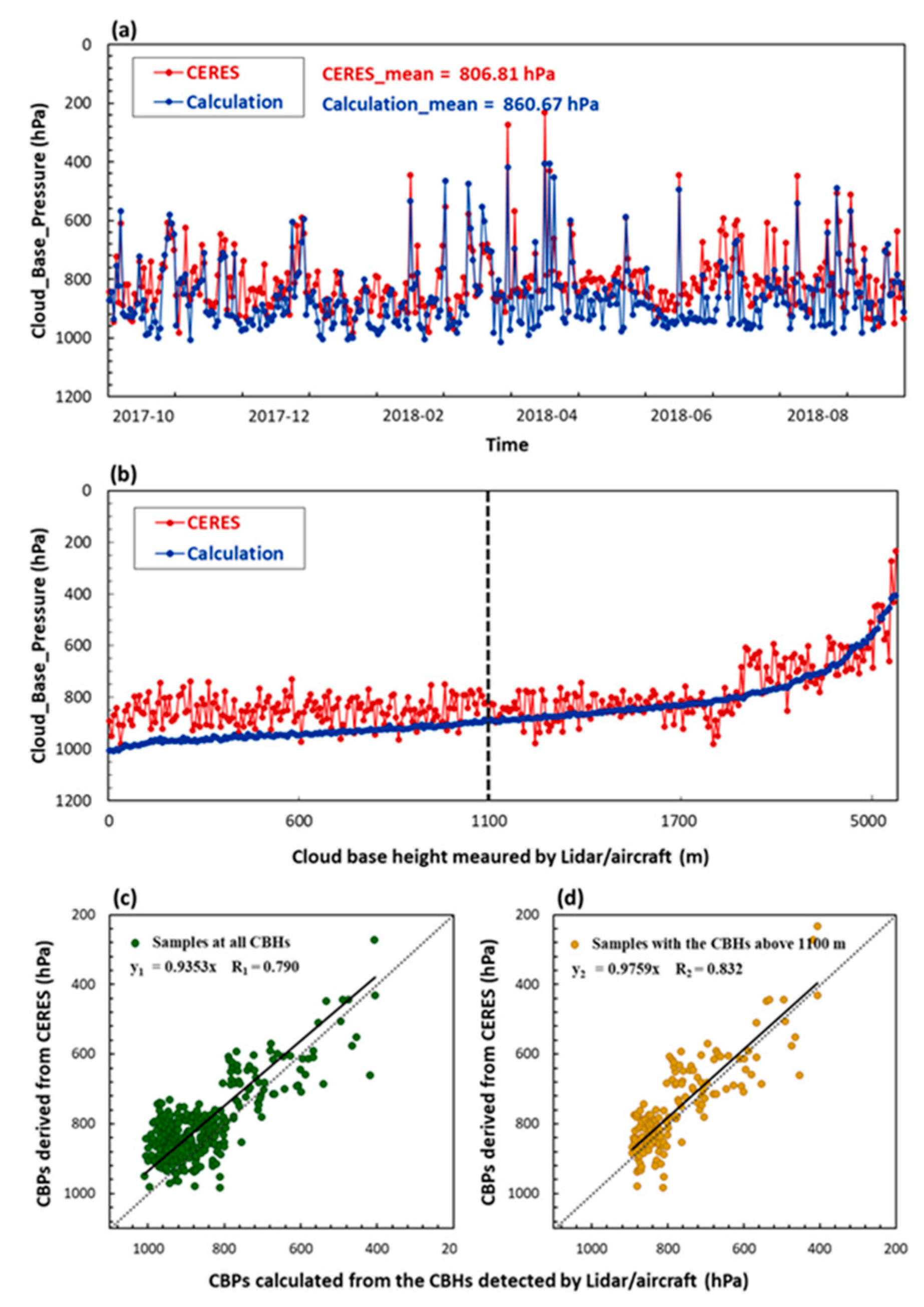
Based on the method described in Section 2.4, a conversion from the CBH in meters to the CBP in hPa was performed. The calculated pressures at the cloud bases were compared with those retrieved from CERES observations, as shown in Figure 5. The time series and a comparison of the CBPs derived from the CERES dataset with the CBPs calculated from ground-based observations are given in Figure 5a. The red and blue lines represent the CBPs obtained from CERES observations and those converted from the Lidar/aircraft measurements, respectively. As shown in Figure 5a, the CBPs from the CERES product were consistently smaller (corresponding higher cloud base) than those calculated from the Lidar/aircraft measurements during a large time period; the averaged CBPs from the CERES product and Lidar/aircraft measurements during the period from October 2017 to September 2018 were 806.81 hPa and 860.67 hPa, respectively. Here, the CBH measurements obtained by Lidar/aircraft were relatively accurate. In this sense, the pressures at the cloud bases observed by CERES could overestimate the CBHs over these sites, which relates to the limited detection ability of passive satellite remote sensing for the cloud base location. Furthermore, according to the geometric heights of the cloud bases measured by Lidar/aircraft, the CBPs obtained from the CERES product were compared with those calculated from the Lidar/aircraft measurements, as shown in Figure 5b. For clouds higher than 1100 m, the CBPs observed by CERES and measured by Lidar/aircraft showed great agreement. However, as shown in Figure 5b, the CERES observations slightly overestimated the cloud base locations in reference to the detection results of Lidar/aircraft, especially for clouds lower than 1100 m. Furthermore, the correlation of CBPs between CERES observations with those calculated by Lidar/aircraft measurements was performed (Figure 5c,d). For the samples of all CBHs (represented by green in Figure 5c), CBPs observed by CERES were significantly smaller than those from Lidar/aircraft measurements (especially for the clouds lower than 1100 m), with a correlation coefficient of 0.790 (significant above the 99% confidence level). However, it was found that the correlation coefficient of the CBPs between CERES observations and the ones calculated from Lidar/aircraft measurements for the clouds higher than 1100 m (represented by yellow in Figure 5d) was 0.832 (significant above the 99% confidence level), which indicates the great agreement of the CERES observations with calculations from Lidar/aircraft measurements.
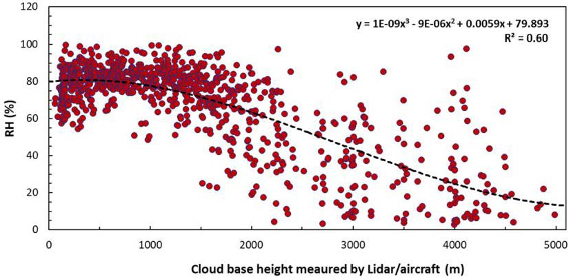
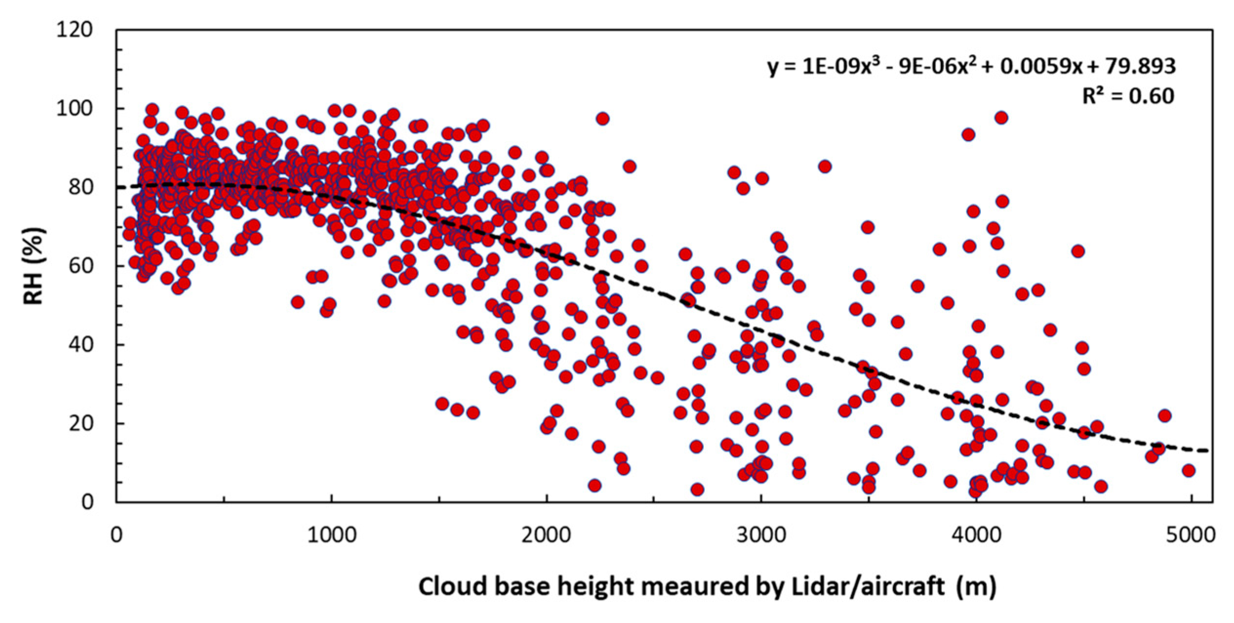
Furthermore, based on the CBPs calculated from the CBHs detected by Lidar/aircraft, the RH values at the cloud base were further extracted from the ERA data. In a sense, the extracted RH values at the cloud base can be regarded as the thresholds for determining the CBHs. Figure 6 shows the correlation between the RHs at the cloud base and the CBHs detected by Lidar/aircraft at the seven sites during the period from October 2017 to September 2018. Overall, most of the RH values at the cloud base ranged from approximately 70 to 90%, where the CBHs were below 2000 m. As the CBH increased from 2000 m, the RH threshold began to decrease to smaller than 60%. As shown in Figure 6, when the CBH was lower than 1000 m, it corresponded to a stable RH threshold of approximately 80%. When the CBH ranged from 1000 to 2000 m, the RH threshold was below 80% and decreased with increasing CBH. However, when the CBH was higher than 2000 m, the RH threshold decreased dramatically with increasing CBH. Additionally, it was found that the samples showed a large scatter and were sparsely distributed in the region with a RH threshold below 60%. Here, the raw values of the RH calculated from the detected CBHs and the RH profiles from the ERA data are illustrated in Figure 6, which presents an uncertainty induced by the RH profiles provided by the ERA data, especially for the clouds at middle and high levels. However, the phenomenon of a relatively low RH threshold for determining the CBHs for relatively high clouds was revealed.
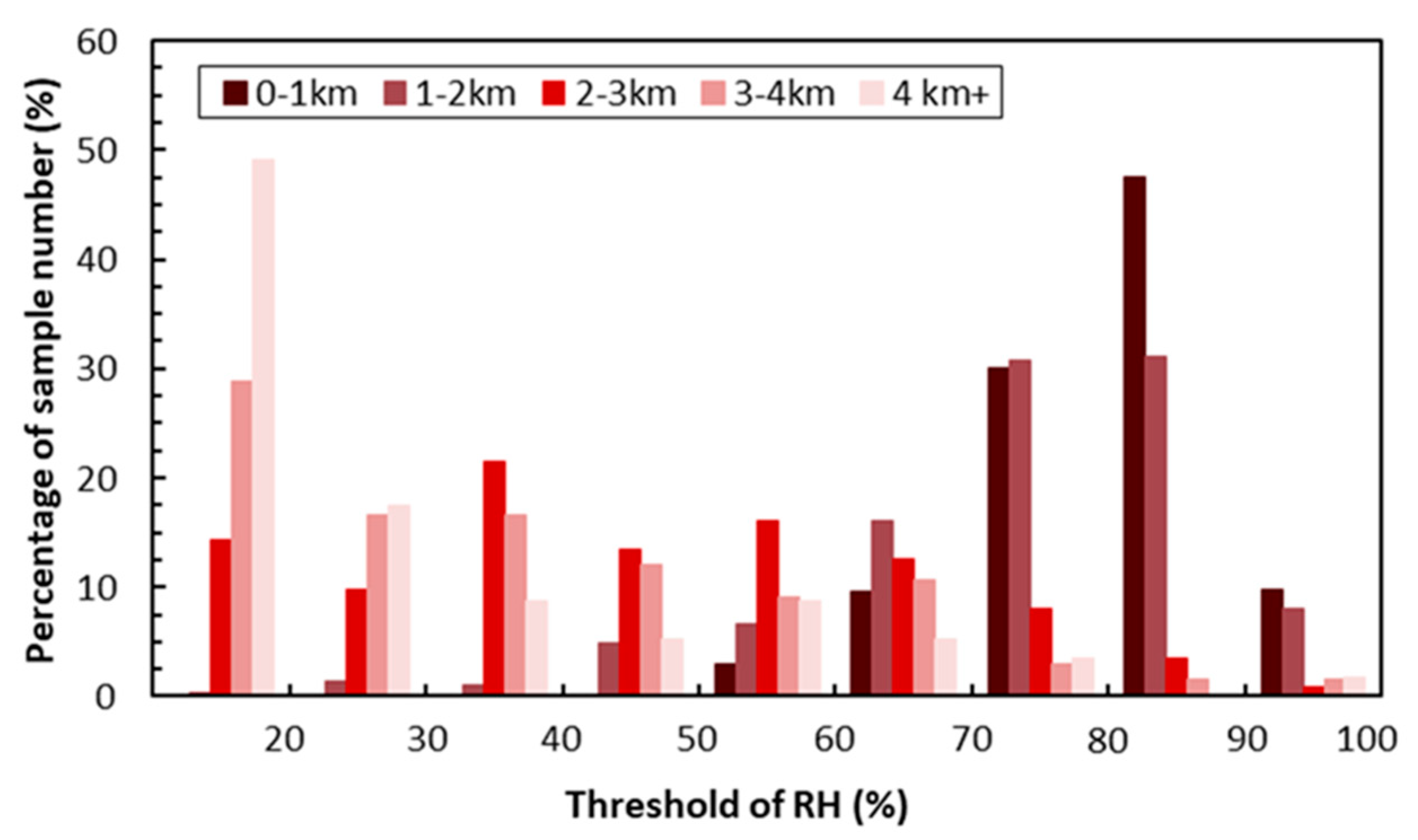
The sample percentages for each RH threshold bin were statistically calculated, as shown in Figure 7. For the clouds with base heights ranging from 0 to 1000 m, the samples were dominantly distributed from 50 to 100%, where the maximum percentage of samples (47.43%) was in the bin ranging from 80 to 90%. For the CBHs ranging from 1000 to 2000 m, the samples were mainly in the RH bins from 20 to 100%, where the maximum percentage of samples (31.01%) was distributed in the bin ranging from 80 to 90%. However, for the clouds with base heights exceeding 3000 m, the samples were mainly distributed in the bins with RHs lower than 50%, where the highest sample percentage (49.12%) was distributed in the RH bin below 20% for CBHs larger than 4000 m.
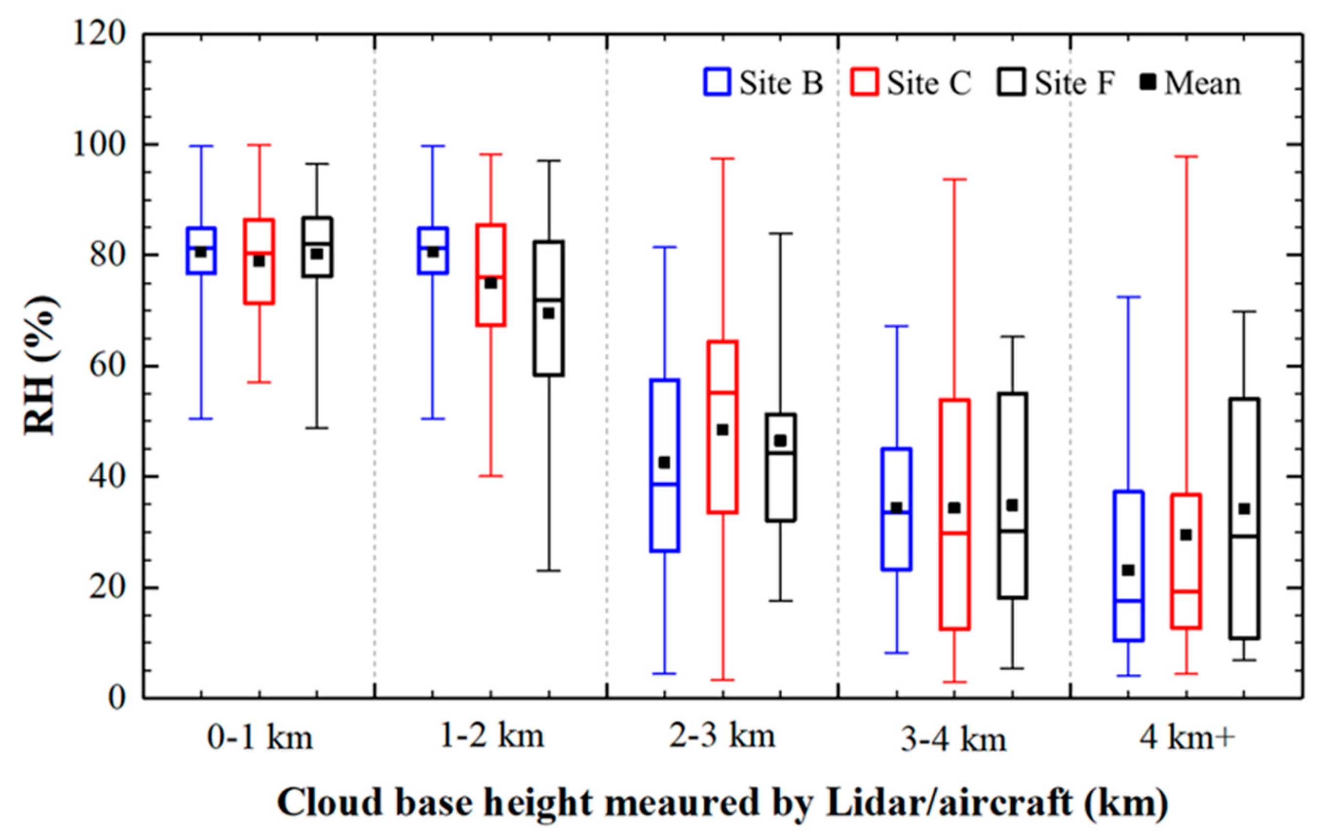
Among the seven sites, the CBH data detected by Lidar/aircraft at sites B, C, and F had better temporal continuity than the CBH data at the other sites during the period from October 2017 to September 2018. Here, an analysis on the RH thresholds for determining the CBHs was performed based on the above three sites (B, C, and F), as shown in Figure 8 (details are in Table 3). As revealed above, the RH thresholds at the three sites ranged approximately from 70 to 90%, where the CBHs were below 2000 m (as shown in the box in Figure 8); the means of the RH thresholds were approximately 80% except for site F (as shown in black squares in Figure 8). As the CBH increased from 2000 m, the RH threshold began to decrease, especially at site C. Overall, the average RH threshold decreased with the increase in CBH. The maximum RH threshold (with a mean of 79.88% for these three sites) was found for the clouds with base heights ranging from 0 to 1000 m. Then, with an increase in the CBH above 1000 m, the average RH threshold decreased and reached the minimum (28.92%) for the CBHs larger than 4000 m. As shown in Figure 8, a significant difference among the RH thresholds for determining the CBHs among the above three sites was mainly observed for the clouds with base heights exceeding 4000 m.
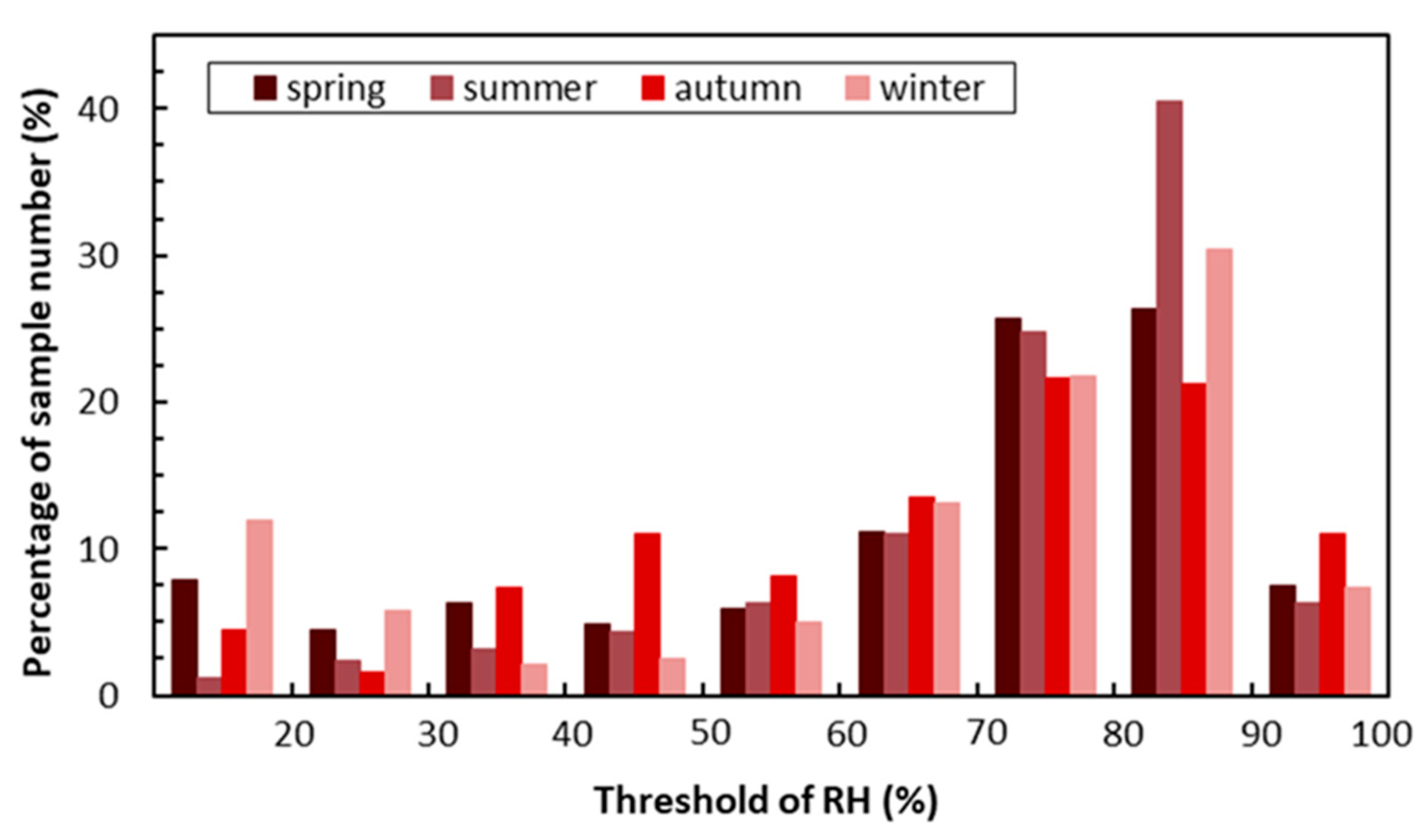
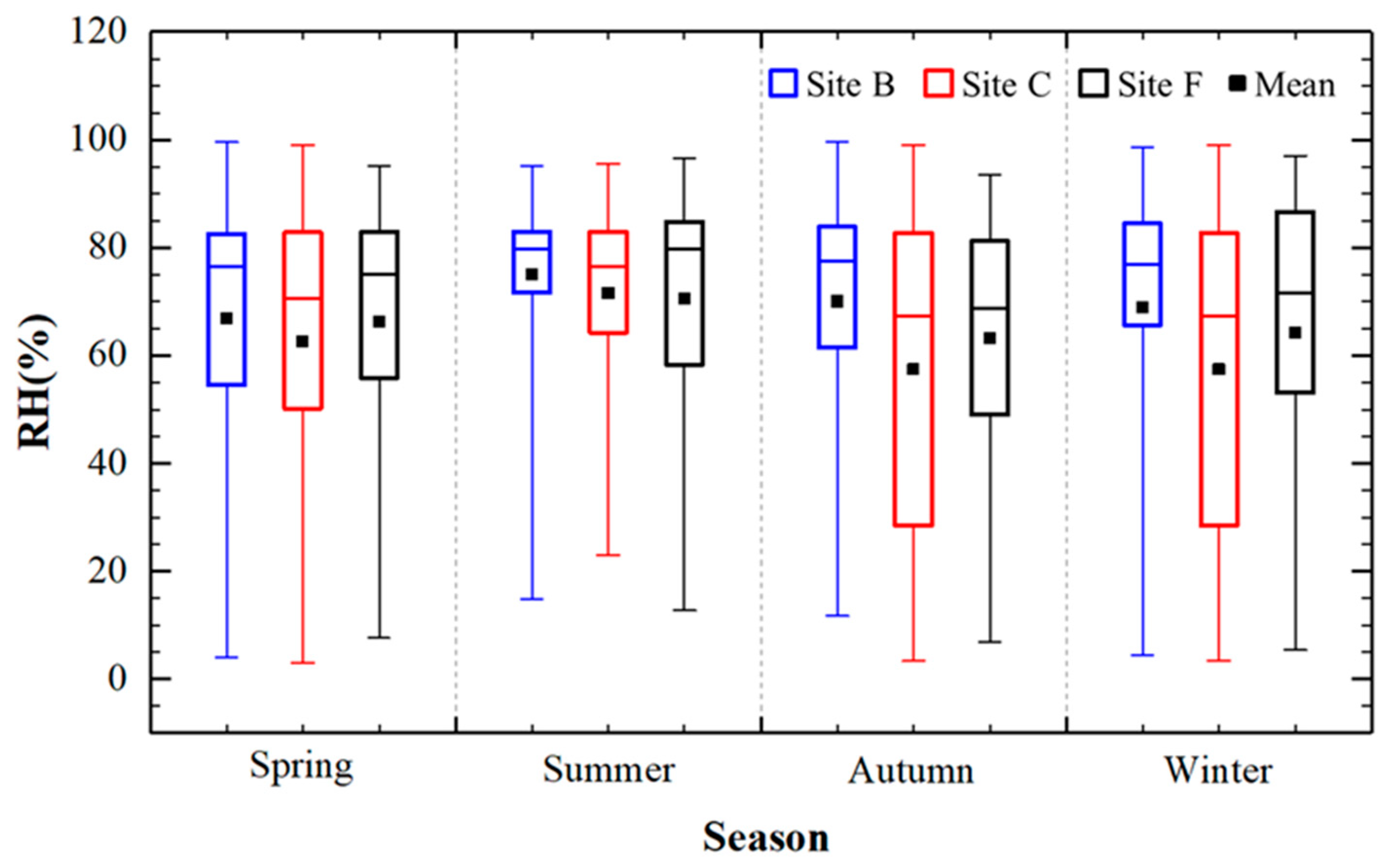
As illustrated above, overall, the RH threshold decreased with an increase in the CBH, especially when the CBH was higher than 2000 m. Furthermore, the seasonal variation of the RH thresholds for determining the CBHs during the period from October 2017 to September 2018 was analyzed. The sample percentages for each RH threshold bin in different seasons are shown in Figure 9. For all seasons, the highest samples were dominantly distributed in the bin from 80 to 90%, where the maximum percentage was 40.55% in the summer. This finding is in agreement with the results in Figure 4. In another sense, for the RH threshold bins larger than 70%, most of the samples were obtained in spring and summer, while the fewest samples were obtained in autumn. However, for the RH threshold bins ranging from 30 to 70%, the samples were mainly collected in the autumn. For the RH threshold bins below 30%, most of the samples were detected in the spring (7.81%) and winter (11.93%). Furthermore, the RH thresholds for determining the CBHs at sites B, C, and F in different seasons were statistically calculated, as shown in Figure 10 (details are in Table 4). This figure shows that the maximum RH threshold (with a mean of 72.39% for sites B, C, and F) was found in the summer, which is consistent with the results shown in Figure 9. Moreover, the average RH thresholds in the spring, autumn, and winter were 65.25%, 66.91%, and 63.56%, respectively. Overall, the RHs at site B indicated slightly higher thresholds than the RHs at sites C and F for all seasons. Furthermore, the RH threshold at site C showed obvious variation in the autumn and winter seasons (as shown in the box in Figure 10), which may be related to the water vapor condition over there.
4. Conclusions
CBH data detected by Lidar, pilot balloon, and aircraft over Southeast China during the period from October 2017 to September 2018 were analyzed in this study. A comparison among the CBHs detected by Lidar, pilot balloon, and aircraft at seven ground-based sites showed that the CBHs observed by Lidar and aircraft were more consistent with a correlation coefficient of 0.86, and thus, the data from Lidar and aircraft were regarded as an accurate reference. During the observational period, the CBHs were higher in the cold months and lower in the warm months; in the latter, most of the CBHs were primarily below 2000 m.
Combined with the RH profiles provided by ERA-Interim data, the RH thresholds were calculated corresponding to the observed CBHs. Overall, the RH threshold was stable at approximately 80% when the CBH was lower than 1000 m; however, with the increase in CBH, the RH threshold began to decrease dramatically, even below 60%, as the CBH was larger than 2000 m. Seasonally, the maximum (72.39%) and minimum (63.56%) RH thresholds were found in the summer and winter, respectively. In addition, the average RH thresholds in the spring and autumn were 65.25% and 66.91%, respectively.
Although some interesting results were found in this study, some uncertainties in the RH threshold calculation based on the profiles from the ERA reanalysis data may be present in the analyses. A huge uncertainty may be induced by the establishment of humidity profiles from ERA reanalysis data. As pointed out by Chernykh and Aldukhov [60], the profile resolution of the reanalysis data could produce some errors in the gradient calculation that forms part of the cloud base determination. Second, the calculation of the CBH, according to the pressure-height formula of polytropic atmosphere, could introduce inevitable errors. Additionally, the RH thresholds for determining the CBHs varied dramatically with the time and CBH, and thus, using an average RH threshold to determine the CBH may conceal some accurate cloud height information. In the future, by combining ground-based and satellite-based observations of the CBH, an artificial neural network method can be used to obtain more accurate CBHs, which will be significantly beneficial to weather forecasting.
Author Contributions
Y.L. designed the paper; Y.T. wrote the original draft; Y.L. and Y.T. wrote, reviewed, and edited; S.H. and Q.Z. helped in data processing; Y.L., Y.T., and R.L. reviewed and revised the paper.
Funding
This research was funded by the Strategic Priority Research Program of the Chinese Academy of Sciences (Grant No. XDA2006010301) and was jointly supported by the National Natural Science Foundation of China (91744311 and 91737101).
Acknowledgments
We acknowledge the CERES (https://ceres.larc.nasa.gov/) and ECMWF (https://www.ecmwf.int/en/forecasts/datasets/reanalysis-datasets/era-interim) science teams for providing excellent and accessible data products that made this study possible. We are also grateful to the ground-based observations from the numerous sites.
Conflicts of Interest
The authors declare no conflicts of interest.
References
- Ramanathan, V.; Cess, R.D.; Harrison, E.F.; Minnis, P.; Barkstrom, B.R.; Ahmad, E.; Hartmann, D. Cloud-radiative forcing and Climate: Results from the earth radiation budget experiment. Science 1989, 243, 57–63. [Google Scholar] [CrossRef] [Green Version]
- Wang, J.H.; Rossow, W.B. Determination of cloud vertical structure from upper-air observations. J. Appl. Meteor. 1995, 34, 2243–2258. [Google Scholar] [CrossRef] [Green Version]
- Sun, B.; Groisman, P.Y. Cloudiness variations over the former Soviet Union. Int. J. Climatol. 2000, 20, 1097–1111. [Google Scholar] [CrossRef]
- Naud, C.M.; Muller, J.P.; Clothiaux, E.E. Comparison between active sensor and radiosonde cloud boundaries over the ARM Southern Great Plains Site. J. Geophys. Res. 2003, 108, 1–12. [Google Scholar] [CrossRef] [Green Version]
- Houghton, J.T.; Ding, Y.; Griggs, D.J.; Noguer, M.; van der Linden, P.J.; Dai, X.; Maskell, K.; Johnson, C.A. Climate Change 2001: The Scientific Basis; Cambridge University Press: New York, NY, USA, 2001; pp. 1–421. [Google Scholar]
- Li, Z.Q.; William, W.K.; Ramanathan, V.; Wu, G.X.; Ding, Y.H.; Madakshira, G.M.; Liu, J.; Qian, Y.F.; Li, J.P.; Zhou, T.J.; et al. Aerosol and Monsoon Climate Interactions over Asia. Rev. Geophys. 2016, 54, 866–929. [Google Scholar] [CrossRef]
- Shang, H.; Letu, H.; Nakajima, T.Y.; Wang, Z.; Ma, R.; Wang, T.; Lei, Y.; Ji, D.; Li, J. Diurnal cycle and seasonal variation of cloud cover over the Tibetan Plateau as determined from Himawari-8 new-generation geostationary satellite data. Sci. Rep. 2018, 8, 1105. [Google Scholar] [CrossRef] [PubMed]
- Letu, H.; Nagao, T.M.; Nakajima, T.Y.; Riedi, J.; Ishimoto, H.; Baran, A.J.; Shang, H.; Sekiguchi, M.; Kikuchi, M. Ice cloud properties from Himawari-8/AHI next-generation geostationary satellite: Capability of the AHI to monitor the DC cloud generation process. IEEE Trans. Geosci. Remote. Sens. 2019, 57, 3229–3239. [Google Scholar] [CrossRef]
- Liu, Y.; Hua, S.; Jia, R.; Huang, J. Effect of aerosols on the ice cloud properties over the Tibetan Plateau. J. Geophys. Res. Atmos. 2019, 124, 9594–9608. [Google Scholar] [CrossRef]
- Huang, J.; Minnis, P.; Lin, B.; Yi, Y.H.; Fan, T.F.; Sun, S.M.; Ayers, J.K. Determination of ice water path in ice-over-water cloud systems using combined MODIS and AMSR-E measurements. Geophys. Res. Lett. 2006, 33, L21801. [Google Scholar] [CrossRef] [Green Version]
- Li, J.; Jian, B.; Huang, J.P.; Hu, Y.; Zhao, C.; Kawamoto, K.; Liao, S.; Wu, M. Long-term variation of cloud droplet number concentrations from space-based Lidar. Remote. Sens. Environ. 2018, 213, 144–161. [Google Scholar] [CrossRef]
- Letu, H.; Nagao, T.M.; Nakajima, T.Y.; Matsumae, Y. Method for validating cloud mask obtained from satellite measurements using ground-based sky camera. Appl. Opt. 2014, 53, 7523–7533. [Google Scholar] [CrossRef] [PubMed]
- Li, J.; Lv, Q.; Zhang, M.; Wang, T.; Kawamoto, K.; Chen, S.; Zhang, B. Effects of atmospheric dynamics and aerosols on the fraction of supercooled water clouds. Atmos. Chem. Phys. 2017, 17, 1847–1863. [Google Scholar] [CrossRef] [Green Version]
- Hua, S.; Liu, Y.; Jia, R.; Chang, S.; Wu, C.; Zhu, Q.; Shao, T.; Wang, B. Role of Clouds in Accelerating Cold-Season Warming During 2000-2015 over the Tibetan Plateau. Int. J. Climatol. 2018, 38, 4950–4966. [Google Scholar] [CrossRef]
- Huang, J.; Minnis, P.; Lin, B.; Wang, T.; Yi, Y.; Hu, Y.; Sun-Mack, S.; Ayers, K. Possible influences of Asian dust aerosols on cloud properties and radiative forcing observed from MODIS and CERES. Geophys. Res. Lett. 2006, 33, L06824. [Google Scholar] [CrossRef] [Green Version]
- Liu, Y.; Huang, J.; Shi, G.; Takamura, T.; Khatri, P.; Bi, J.; Shi, J.; Wang, T.; Wang, X.; Zhang, B. Aerosol optical properties and radiative effect determined from sky-radiometer over Loess Plateau of Northwest China. Atmos. Chem. Phys. 2011, 11, 11455–11463. [Google Scholar] [CrossRef] [Green Version]
- Li, Z.; Guo, J.; Ding, A.; Liao, H.; Liu, J.; Sun, Y.; Wang, T.; Xue, H.; Zhang, H.; Zhu, B. Aerosol and boundary-layer interactions and impact on air quality. Natl. Sci. Rev. 2017, 4, 810–833. [Google Scholar] [CrossRef]
- Li, J.; Huang, J.; Stamnes, K.; Wang, T.; Lv, Q.; Jin, H. A global survey of cloud overlap based on CALIPSO and CloudSat measurements. Atmos. Chem. Phys. 2015, 15, 519–536. [Google Scholar] [CrossRef] [Green Version]
- Chen, S.; Jiang, N.; Huang, J.; Zang, Z.; Guan, X.; Ma, X.; Luo, Y.; Li, J.; Zhang, X.; Zhang, Y. Estimations of indirect and direct anthropogenic dust emission at the global scale. Atmos. Environ. 2018, 200, 50–60. [Google Scholar] [CrossRef]
- Guo, J.; Liu, H.; Li, Z.; Rosenfeld, D.; Jiang, M.; Xu, W.; Jiang, J.; He, J.; Chen, D.; Min, M.; et al. Aerosol-induced changes in the vertical structure of precipitation: A perspective of TRMM precipitation radar. Atmos. Chem. Phys. 2018, 18, 13329–13343. [Google Scholar] [CrossRef] [Green Version]
- Zhu, Q.; Liu, Y.; Jia, R.; Hua, S.; Shao, T.; Wang, B. A numerical simulation study on the impact of smoke aerosols from Russian forest fires on the air pollution over Asia. Atmos. Environ. 2018, 182, 263–274. [Google Scholar] [CrossRef]
- Guo, J.; Deng, M.; Lee, S.S.; Wang, F.; Li, Z.; Zhai, P.; Liu, H.; Lv, W.; Yao, W.; Li, X. Delaying precipitation and lightning by air pollution over the Pearl River Delta. Part I: Observational analyses. J. Geophys. Res. Atmos. 2016, 121, 6472–6488. [Google Scholar] [CrossRef]
- Liu, Y.; Zhu, Q.; Huang, J.; Hua, S.; Jia, R. Impact of dust-polluted convective clouds over the Tibetan Plateau on downstream precipitation. Atmos. Environ. 2019, 209, 67–77. [Google Scholar] [CrossRef]
- Stephens, G. Cloud feedbacks in the climate system: A critical review. J. Clim. 2005, 18, 237–273. [Google Scholar] [CrossRef] [Green Version]
- Leyton, S.M.; Fritsch, J.M. The impact of high-frequency surface weather observations on short-term probabilistic forecasts of ceiling and visibility. J. Appl. Meteorol. 2004, 43, 145–156. [Google Scholar] [CrossRef]
- Inoue, M.; Fraser, A.D.; Phillips, H.E. An assessment of numerical weather prediction–derived low-cloud-base height forecasts. Wea. Forecast. 2015, 30, 486–497. [Google Scholar] [CrossRef] [Green Version]
- Costa-Surós, M.; Calbó, J.; González, J.A.; Martin-Vide, J. Behavior of cloud base height from ceilometer measurements. Atmos. Res. 2013, 127, 64–76. [Google Scholar] [CrossRef] [Green Version]
- L’Ecuyer, T.S.; Jiang, J. Touring the atmosphere aboard the A-Train. Phys. Today 2010, 63, 36–41. [Google Scholar] [CrossRef] [Green Version]
- Leeuw, G.; Kokhanovsky, A.; Cermak, J. Remote sensing of aerosols and clouds: Techniques and applications (editorial to special issue in Atmospheric Research). Atmos. Res. 2012, 113, 40–42. [Google Scholar] [CrossRef]
- Hutchison, K.D. The retrieval of cloud base heights from MODIS and three-dimensional cloud fields from NASA’s EOS Aqua mission. Int. J. Remote. Sens. 2002, 23, 5249–5265. [Google Scholar] [CrossRef]
- Hutchison, K.D.; Wong, E.; Ou, S.C. Cloud base heights retrieved during night-time conditions with MODIS data. Int. J. Remote. Sens. 2006, 27, 2847–2862. [Google Scholar] [CrossRef]
- Kuji, M.; Nakajima, T.Y.; Mukai, S. Retrieval of cloud geometrical properties using optical remote sensing data. Proc. SPIE 2000. [Google Scholar] [CrossRef]
- Borg, L.A.; Holz, R.E.; Turner, D.D. Investigating cloud radar sensitivity to optically thin cirrus using collocated Raman lidar observations. Geophys. Res. Lett. 2011, 38, L05807. [Google Scholar] [CrossRef]
- Sharma, S.; Vaishnav, R.; Shukla, M.V.; Kumar, P.; Thapliyal, P.K.; Lal, S.; Acharya, Y.B. Evaluation of cloud base height measurements from Ceilometer CL31 and MODIS satellite over Ahmedabad, India. Atmos. Meas. Technol. 2015, 8, 11729–11752. [Google Scholar] [CrossRef]
- Liang, Y.; Sun, X.; Miller, S.D.; Li, H.; Zhou, Y.; Zhang, R.; Li, S. Cloud Base Height Estimation from ISCCP Cloud-Type Classification Applied to A-Train Data. Adv. Meteorol. 2017. [Google Scholar] [CrossRef] [Green Version]
- Oh, S.B.; Kim, Y.H.; Cho, C.H.; Lim, E. Verification and correction of cloud base and top height retrievals from Ka-band cloud radar in Boseong, Korea. Adv. Atmos. Sci. 2016, 33, 73–84. [Google Scholar] [CrossRef]
- Zhang, J.Q.; Xia, X.A.; Chen, H.B. A comparison of cloud layers from ground and satellite active remote sensing at the Southern Great Plains ARM site. Adv. Atmos. Sci. 2017, 34, 347–359. [Google Scholar] [CrossRef]
- Martucci, G.; Milroy, C.; O’Dowd, C.D. Detection of cloud-base height using Jenoptik CHM15K and Vaisala CL31 ceilometers. J. Atmos. Ocean. Technol. 2010, 27, 305–318. [Google Scholar] [CrossRef]
- Poore, K.D.; Wang, J.; Rossow, W.B. Cloud layer thicknesses from a combination of surface and upper-air observations. J. Clim. 1995, 8, 550–568. [Google Scholar] [CrossRef] [Green Version]
- Yan, W.; Han, D.; Lu, W.; Lei, X. Research of cloud base height retrieval based on COSMIC occultation sounding data. Chin. J. Geophys. 2012, 55, 1–15. [Google Scholar] [CrossRef]
- Zhang, J.; Chen, H.; Li, Z.; Fan, X.; Peng, L.; Yu, Y.; Cribb, M. Analysis of cloud layer structure in Shouxian, China using RS92 radiosonde aided by 95 GHz cloud radar. J. Geophys. Res. 2010, 115, D00K30. [Google Scholar] [CrossRef]
- Zhang, Y.; Zhang, L.; Guo, J.; Feng, J.; Cao, L.; Wang, Y.; Zhou, Q.; Li, L.; Li, B.; Xu, H.; et al. Climatology of cloud-base height from long-term radiosonde measurements in China. Adv. Atmos. Sci. 2018, 35, 158–168. [Google Scholar] [CrossRef]
- Kassianov, E.I.; Long, C.N.; Christy, J. Cloud-Base-Height Estimation from Paired Ground-Based Hemispherical Observations. J. Appl. Meteorol. 2005, 44, 1221–1233. [Google Scholar] [CrossRef]
- Maturilli, M.; Ebell, K. Twenty-five years of cloud base height measurements by ceilometer in Ny-Ålesund, Svalbard. Earth Syst. Sci. Data 2018, 10, 1451–1456. [Google Scholar] [CrossRef] [Green Version]
- Wang, Z.; Wang, Z.H.; Cao, X. Consistency analysis for cloud vertical structure derived from millimeter cloud radar and radiosonde profiles. Acta. Meteorol. Sin. 2016, 74, 815–826. [Google Scholar]
- Forsythe, J.; Haar, T.V.; Reinke, D. Cloud-base height estimates using a combination of meteorological satellite imagery and surface reports. J. Appl. Meteorol. 2000, 39, 2336–2347. [Google Scholar] [CrossRef]
- Barker, H.W. Estimating cloud field albedo using one-dimensional series of optical depth. J. Atmos. Sci. 1996, 53, 2826–2837. [Google Scholar] [CrossRef]
- Berg, L.; Stull, R. Accuracy of point and line measures of boundary layer cloud amount. J. Appl. Meteor. 2002, 41, 640–650. [Google Scholar] [CrossRef]
- Kassianov, E.I.; Long, C.; Ovtchinnikov, M. Cloud sky cover versus cloud fraction: Whole-sky simulations and observations. J. Appl. Meteor. 2005, 44, 86–98. [Google Scholar] [CrossRef]
- Chernykh, I.V.; Eskridge, R.E. Determination of cloud amount and level from radiosonde soundings. J. Appl. Meteorol. 1996, 35, 1362–1369. [Google Scholar] [CrossRef]
- Craven, J.P.; Jewell, R.E.; Brooks, H.E. Comparison between observed convective cloud-base heights and lifting condensation level for two different lifted parcels. Wea. Forecast. 2002, 17, 885–890. [Google Scholar] [CrossRef] [Green Version]
- Stull, R.B.; Eloranta, E. A case study of the accuracy of routine, fair-weather cloud-base reports. Natl. Wea. Dig. 1985, 10, 19–24. [Google Scholar]
- Zhang, Y.; Klein, S.A. Factors controlling the vertical extent of fair-weather shallow cumulus clouds over land: Investigation of diurnal-cycle observations collected at the ARM Southern Great Plains site. J. Atmos. Sci. 2013, 70, 1297–1315. [Google Scholar] [CrossRef]
- Romps, D.M. Exact expression for the lifting condensation level. J. Atmos. Sci. 2017, 74, 3891–3900. [Google Scholar] [CrossRef]
- Kleet, J.D. Stable analytical inversion solution for processing lidar returns. Appl. Opt. 1981, 20, 211–220. [Google Scholar] [CrossRef] [PubMed] [Green Version]
- Collis, R.T.H.; Russell, P.B. Lidar measurement of particles and gases by elastic backscateringand dif ferential absorption. In Laser Monitoring of the Atmosphere; Springer: Berlin/Heidelberg, Germany, 1976; pp. 71–151. [Google Scholar]
- Chambers, L.H.; Lin, B.; Young, D.F. Examination of new CERES data for evidence of tropical iris feedback. J. Clim. 2002, 15, 3719–3726. [Google Scholar] [CrossRef]
- Dee, D.P.; Uppala, S.M.; Simmons, A.J.; Berrisford, P.; Poli, P.; Kobayashi, S.; Andrae, U.; Balmaseda, M.A.; Balsamo, G.; Bauer, P.; et al. The ERA-Interim reanalysis: Configuration and performance of the data assimilation system. Quart. J. R. Meteor. Soc. 2011, 137, 553–597. [Google Scholar] [CrossRef]
- Iribarne, J.V.; Cho, H.-R. Atmospheric Physics; Reidel: Dordrecht, The Netherlands, 1980; ISBN 90-277-1033-3. [Google Scholar]
- Chernykh, I.; Aldukhov, O. Vertical distribution of cloud layers from atmospheric radiosounding data. Izv. Atmos. Ocean. Phys. 2004, 40, 41–53. [Google Scholar]
Figure 1.
Distribution of the annual mean cloud fraction (unit: %) derived from Clouds and the Earth’s Radiant Energy System (CERES) product in the period from October 2017 to September 2018 and the distribution of observational sites for the cloud base height (CBH) in Southeast China. The blue triangles denote the ground-based observational sites for the CBH.

Figure 2.
Scatter-grams of the Lidar/pilot-balloon observed and aircraft sounded CBHs at sites in Southeast China. The red and blue squares denote the CBHs from the pilot balloon and cloud Lidar, respectively.
Figure 2.
Scatter-grams of the Lidar/pilot-balloon observed and aircraft sounded CBHs at sites in Southeast China. The red and blue squares denote the CBHs from the pilot balloon and cloud Lidar, respectively.

Figure 3.
Seasonal variation of the mean CBH detected by cloud Lidar and aircraft during the period from October 2017 to September 2018 at seven ground-based sites. The light cyan bar represents the number of samples at each site in four seasons. Error bars represent the confidence levels of the mean values, assuming independent data. Errors are calculated as , where is the sample number of CBH measurements within the season and is the standard deviation.

Figure 4.
(a) Monthly and (b) diurnal variations of the CBH during the period from October 2017 to September 2018. Black line in (a) represents the average CBH at all sites. Green line in (b) denotes the average CBH at sites A and B. Error bars represent the confidence levels of the mean values, assuming independent data. Errors were calculated as , where is the sample number of CBH measurements within the season and is the standard deviation.

Figure 5.
(a) Time series and (b) comparison of the CBPs derived from CERES observations with those calculated from the CBHs detected by Lidar/aircraft at site B during the period from October 2017 to September 2018. Correlation between the CBPs derived from CERES observations with those calculated from Lidar/aircraft measurements for samples of (c) all CBHs and (d) CBHs above 1100 m at site B during the period from October 2017 to September 2018.

Figure 6.
Correlation between the RHs at the cloud base and the CBHs detected by Lidar/aircraft at all sites during the period from October 2017 to September 2018. The black dashed line denotes the fitting result with a cubic polynomial.
Figure 6.
Correlation between the RHs at the cloud base and the CBHs detected by Lidar/aircraft at all sites during the period from October 2017 to September 2018. The black dashed line denotes the fitting result with a cubic polynomial.

Figure 7.
Distribution of the sample number percentage (unit: %) in each RH threshold bin for various CBHs measured by Lidar/aircraft at sites B, C, and F during the period from October 2017 to September 2018.
Figure 7.
Distribution of the sample number percentage (unit: %) in each RH threshold bin for various CBHs measured by Lidar/aircraft at sites B, C, and F during the period from October 2017 to September 2018.

Figure 8.
Statistics on the RH threshold for the clouds with different height at sites B, C, and F during the period from October 2017 to September 2018. Whiskers cover the range of RH thresholds. The upper, middle, and lower lines of the box correspond to the first, second, and third quartiles (the 75th, 50th, and 25th percentiles). Black squares denote the means of RH threshold.

Figure 9.
Seasonal distribution of the sample number percentage (unit: %) in each RH threshold bin for various CBHs measured by Lidar/aircraft at sites B, C, and F during the period from October 2017 to September 2018.
Figure 9.
Seasonal distribution of the sample number percentage (unit: %) in each RH threshold bin for various CBHs measured by Lidar/aircraft at sites B, C, and F during the period from October 2017 to September 2018.

Figure 10.
Seasonal statistics on the RH threshold for determining the CBHs at sites B, C, and F during the period from October 2017 to September 2018. Whiskers cover the range of RH thresholds. The upper, middle, and lower lines of the box correspond to the first, second, and third quartiles (the 75th, 50th, and 25th percentiles). Black squares denote the means of RH threshold.


Table 1.
Information on the observational sites for the cloud base height (CBH).
| Site | Location | Elevation (m; Above Sea Level) | Number of Samples | ||
|---|---|---|---|---|---|
| Aircraft | Lidar | Pilot Balloon | |||
| A | (117° E, 25° N) | 397 | 12 | 3268 | 230 |
| B | (116° E, 23° N) | 13.8 | 58 | 2854 | 161 |
| C | (115° E, 28° N) | 16 | 60 | 300 | 168 |
| D | (120° E, 26° N) | 366.6 | 45 | 1748 | 182 |
| E | (118° E, 34° N) | 15.7 | 75 | 76 | 19 |
| F | (120° E, 30° N) | 4.1 | 28 | 177 | 23 |
| G | (121° E, 31° N) | 4.4 | 50 | 47 | 24 |
Table 2.
Technical specifications of the cloud Lidar.
| Parameter Name | Parameter Value |
|---|---|
| Laser | InGaAs (a semiconductor laser) |
| Wavelength | 905 ± 10 nm |
| Single laser pulse energy | ≤20 μJ |
| Pulse width | 45 ns ± 10 ns |
| Scattering angle of laser beam | ≤3 mrad |
| Pulse repetition frequency | 1 kHz ± 15% |
| Effective aperture of the optical system | 102 mm |
| Interferometric filter | 910 ± 15 nm |
Table 3.
Characteristics of the relative humidity thresholds of the CBH (unit: %).
| Altitude of the Cloud Base | Site B | Site C | Site F | Number of Samples | Mean Threshold |
|---|---|---|---|---|---|
| ≤1 km | 80.54 | 78.90 | 80.21 | 415 | 79.88 |
| 1–2 km | 76.04 | 74.91 | 72.44 | 337 | 74.46 |
| 2–3 km | 42.56 | 48.50 | 46.51 | 110 | 45.86 |
| 3–4 km | 34.36 | 34.32 | 34.84 | 64 | 34.51 |
| >4 km | 23.11 | 29.53 | 34.12 | 56 | 28.92 |
Table 4.
Seasonal average of the relative humidity thresholds of the CBH (unit: %).
| Seasons | Site B | Site C | Site F | Number of Samples | Mean Threshold |
|---|---|---|---|---|---|
| Spring | 66.89 | 62.56 | 66.31 | 269 | 65.25 |
| Summer | 75.09 | 71.58 | 70.51 | 254 | 72.39 |
| Autumn | 70.52 | 64.88 | 65.32 | 262 | 66.91 |
| Winter | 68.93 | 57.46 | 64.28 | 243 | 63.56 |
© 2019 by the authors. Licensee MDPI, Basel, Switzerland. This article is an open access article distributed under the terms and conditions of the Creative Commons Attribution (CC BY) license (http://creativecommons.org/licenses/by/4.0/).
Share and Cite
MDPI and ACS Style
Liu, Y.; Tang, Y.; Hua, S.; Luo, R.; Zhu, Q. Features of the Cloud Base Height and Determining the Threshold of Relative Humidity over Southeast China. Remote Sens. 2019, 11, 2900. https://0-doi-org.brum.beds.ac.uk/10.3390/rs11242900
AMA Style
Liu Y, Tang Y, Hua S, Luo R, Zhu Q. Features of the Cloud Base Height and Determining the Threshold of Relative Humidity over Southeast China. Remote Sensing. 2019; 11(24):2900. https://0-doi-org.brum.beds.ac.uk/10.3390/rs11242900
Chicago/Turabian StyleLiu, Yuzhi, Yuhan Tang, Shan Hua, Run Luo, and Qingzhe Zhu. 2019. "Features of the Cloud Base Height and Determining the Threshold of Relative Humidity over Southeast China" Remote Sensing 11, no. 24: 2900. https://0-doi-org.brum.beds.ac.uk/10.3390/rs11242900
Note that from the first issue of 2016, this journal uses article numbers instead of page numbers. See further details here.