Combining Earth Observations, Cloud Computing, and Expert Knowledge to Inform National Level Degradation Assessments in Support of the 2030 Development Agenda


Abstract
:1. Introduction
2. Materials and Methods
2.1. Study Area
2.2. Time Series of Earth Observation Data
2.3. Trends in Land Productivity
2.4. Categorization of Trend Intensity
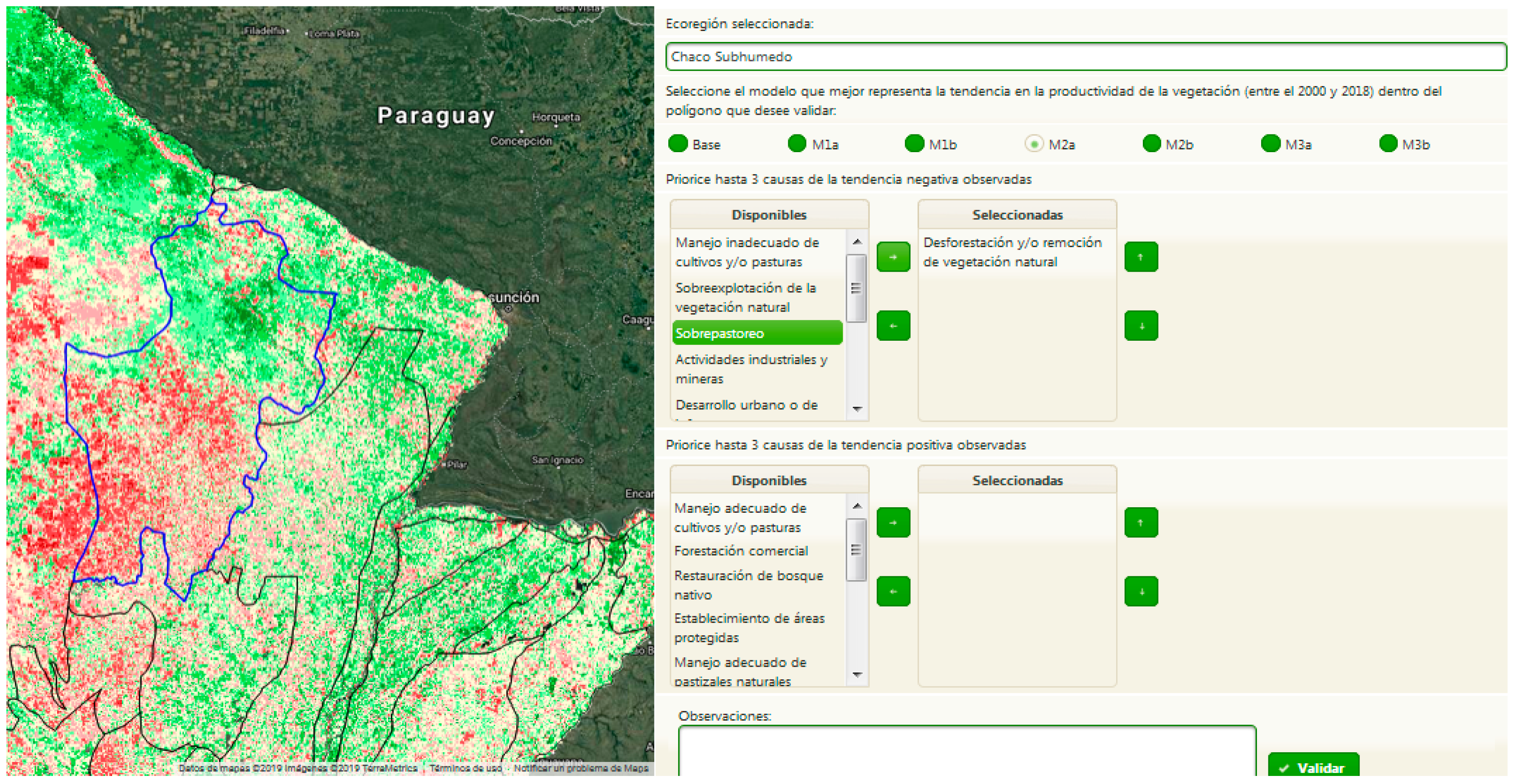
2.5. Online Application for Expert Data Collection
2.6. Comparison of Indicators’ Ability to Detect Decreases in Primary Productivity in Plots with Forest Loss
3. Results
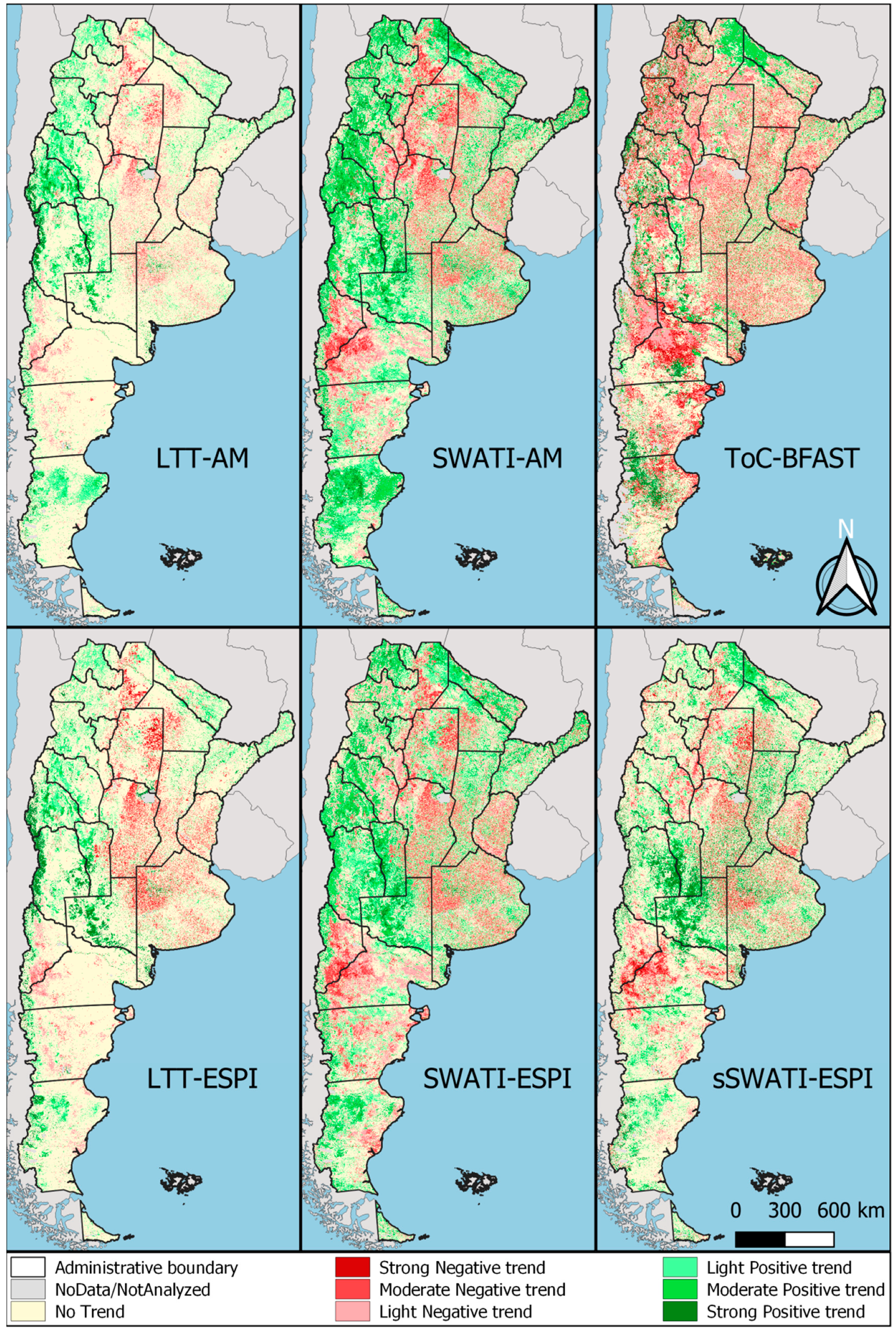
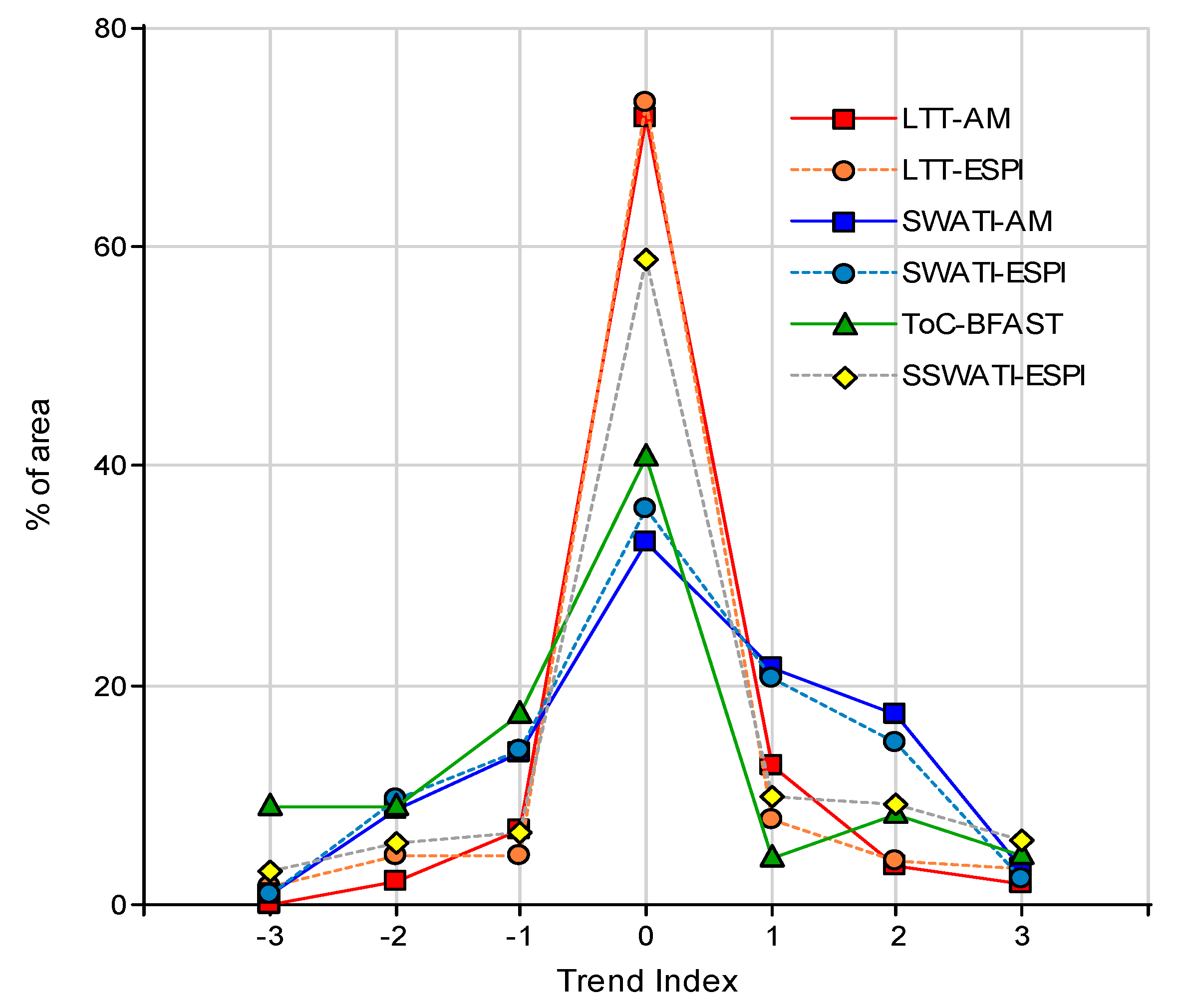
3.1. Trends in Land Productivity
3.2. Expert Opinion Results
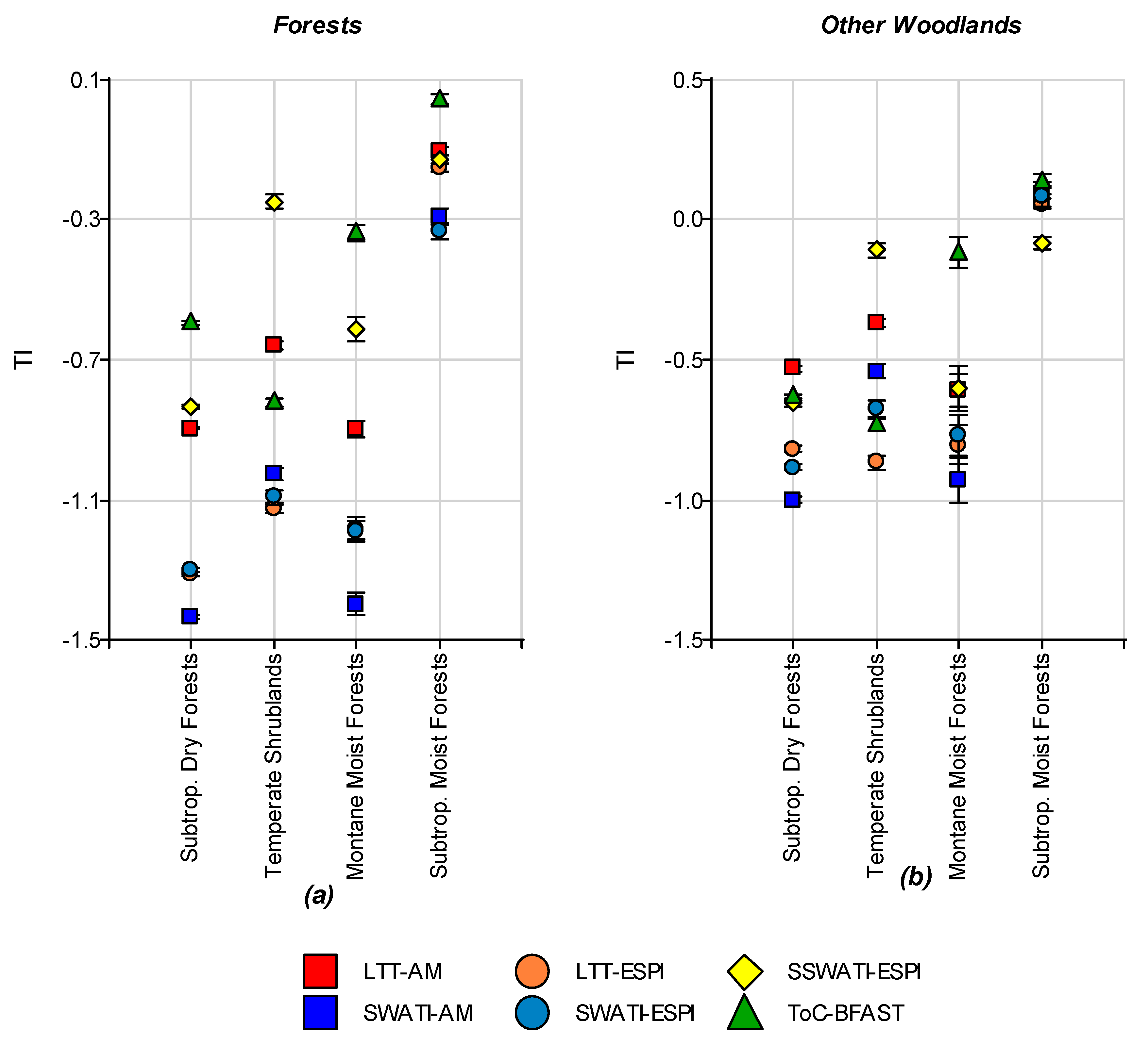
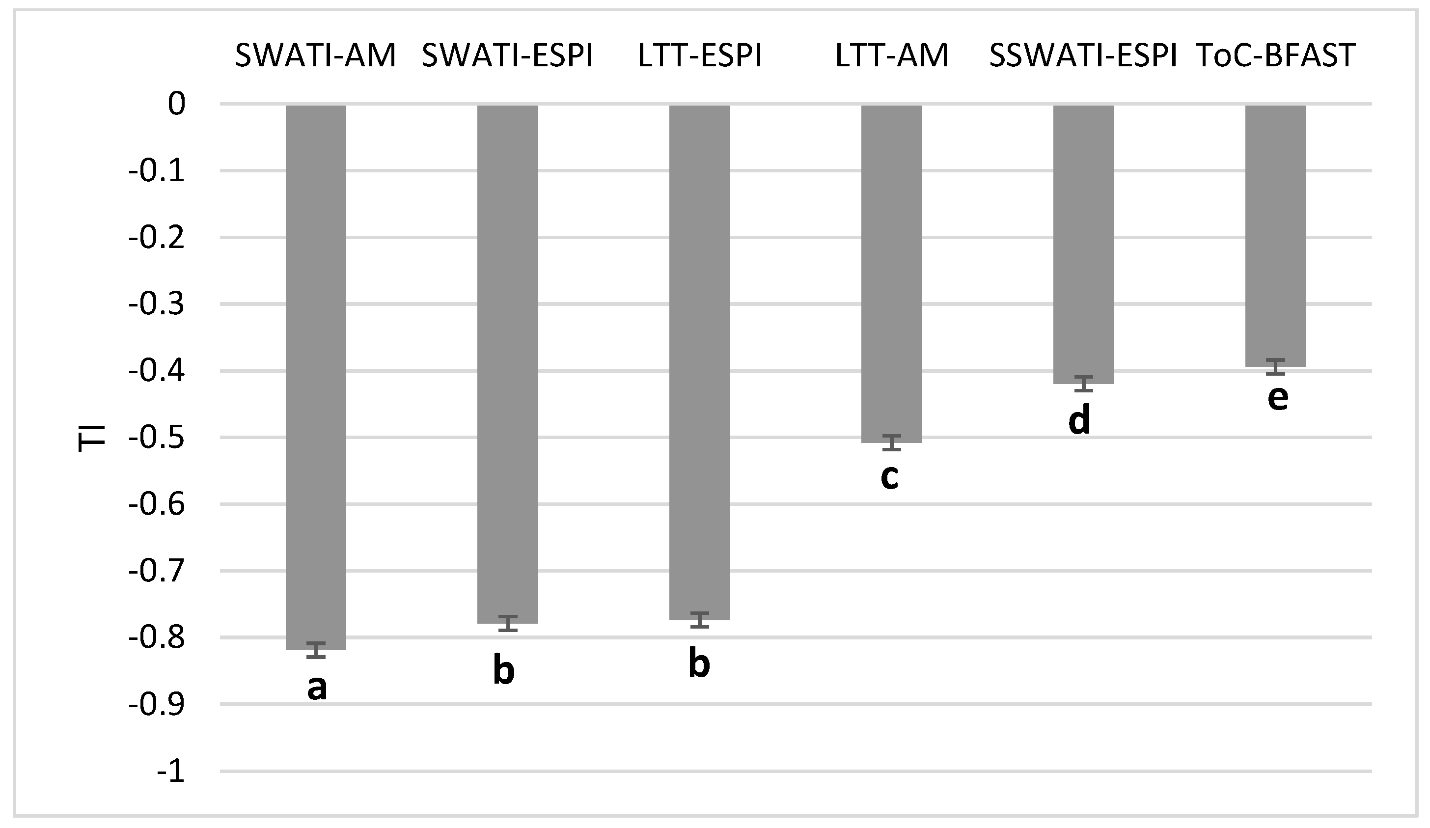
3.3. Detection of Negative Primary Productivity Trends in Plots with Forest Loss
4. Discussion
5. Conclusions
Supplementary Materials
Author Contributions
Funding
Acknowledgments
Conflicts of Interest
Appendix A


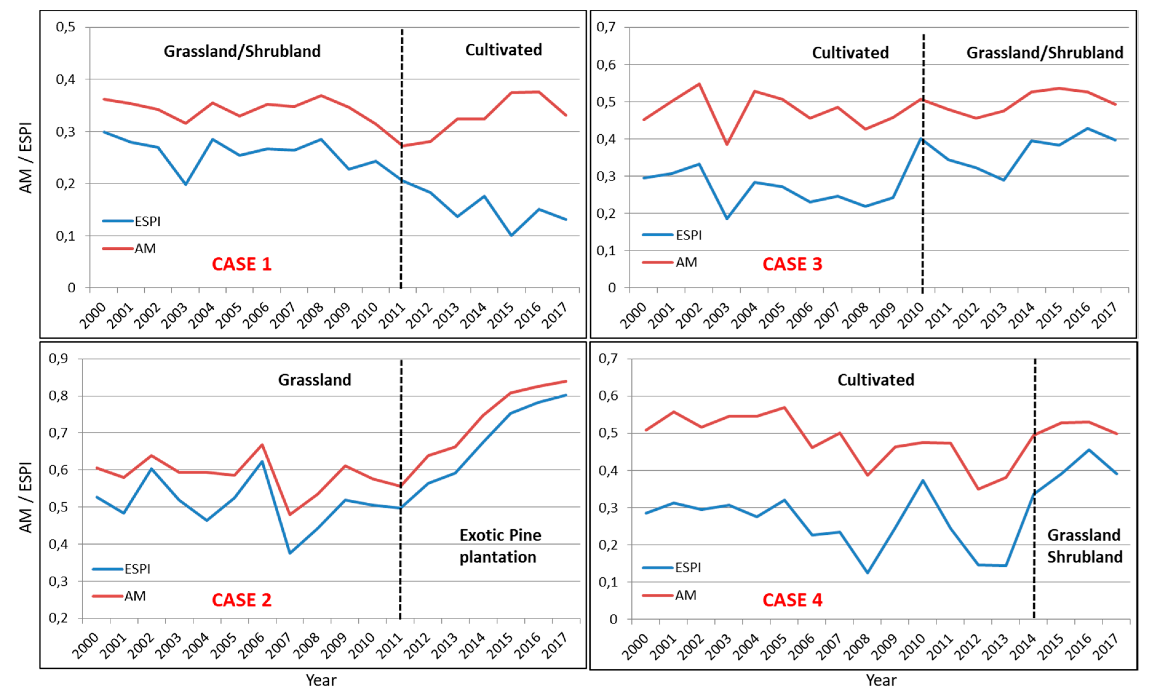
| Indicator | Value | Trend Intensity | Value | Trend Intensity | ||
|---|---|---|---|---|---|---|
| CASE 1 | CASE 3 | |||||
| LTT-AM | −4% | 0 | No trend | 8% | 0 | No trend |
| LTT-ESPI | −58% | 3 | Strong negative | 62% | 3 | Strong positive |
| SWATI-AM | −1 | 1 | Light negative | 0 | 0 | No trend |
| SWATI-ESPI | −3 | 2 | Moderate negative | 2 | 2 | Moderate positive |
| ToC-BFAST | −1 | 1 | Light negative | 1 | 1 | Light positive |
| SSWATI-ESPI | −39% | 2 | Moderate negative | 52% | 3 | Strong positive |
| CASE 2 | CASE 4 | |||||
| LTT-AM | 43% | 2 | Moderate positive | −11% | 0 | No trend |
| LTT-ESPI | 64% | 3 | Strong positive | 23% | 0 | No trend |
| SWATI-AM | 3 | 2 | Moderate positive | 1 | 1 | Light positive |
| SWATI-ESPI | 3 | 2 | Moderate positive | 1 | 1 | Light positive |
| ToC-BFAST | 0 | 0 | No trend | 0 | 0 | No trend |
| SSWATI-ESPI | 60% | 3 | Strong positive | 106% | 3 | Strong positive |
| Ecoregion | TI | LTT-AM | LTT-ESPI | SWATI-AM | SWATI-ESPI | ToC-BFAST | SSWATI-ESPI | Average |
|---|---|---|---|---|---|---|---|---|
| Argentina | −3 | 0.09 | 1.68 | 1.04 | 0.93 | 8.97 | 3.05 | 2.6 |
| −2 | 2.08 | 4.45 | 8.57 | 9.7 | 8.96 | 5.69 | 6.6 | |
| −1 | 6.73 | 4.47 | 13.85 | 14.11 | 17.42 | 6.58 | 10.5 | |
| 0 | 71.84 | 73.21 | 33.17 | 36.17 | 40.77 | 58.79 | 52.3 | |
| 1 | 12.62 | 7.72 | 21.59 | 20.75 | 4.22 | 9.75 | 12.8 | |
| 2 | 3.57 | 3.89 | 17.38 | 14.85 | 8.27 | 9.15 | 9.5 | |
| 3 | 1.84 | 3.35 | 3.18 | 2.28 | 4.45 | 5.78 | 3.5 | |
| ND | 1.21 | 1.21 | 1.21 | 1.21 | 6.94 | 1.21 | 2.2 | |
| Altoandina (Montane Grasslands and Shrublands) | −3 | 1.8 | 1 | 6.5 | 8.9 | 4.3 | 2.5 | 3.8 |
| −2 | 0.2 | 0.3 | 2.2 | 1.9 | 2.7 | 1.7 | 1.2 | |
| −1 | 0.1 | 0.1 | 0.1 | 0.1 | 9.6 | 2.8 | 1.7 | |
| 0 | 53 | 58.3 | 31.1 | 34.7 | 19.7 | 67.3 | 32.8 | |
| 1 | 17.7 | 9.1 | 14.5 | 14.4 | 2.1 | 5.8 | 9.6 | |
| 2 | 8.5 | 6.2 | 38.9 | 35.7 | 3.4 | 5.5 | 15.5 | |
| 3 | 16.8 | 23.1 | 4.9 | 2.5 | 6.7 | 12.4 | 9.0 | |
| ND | 1.9 | 1.9 | 1.9 | 1.9 | 51.5 | 1.9 | 9.9 | |
| Chaco (Subtropical Grasslands, Savannas, and Shrublands) | −3 | 8.5 | 3.7 | 18.9 | 14.2 | 25.2 | 8.3 | 11.8 |
| −2 | 4.3 | 5.6 | 12.4 | 10.9 | 9.3 | 6.7 | 7.1 | |
| −1 | 0.2 | 3.2 | 2 | 1.2 | 5.8 | 3.7 | 2.1 | |
| 0 | 70.8 | 72.7 | 32 | 32.6 | 37.2 | 54.4 | 40.9 | |
| 1 | 12.7 | 9.2 | 16.9 | 23.2 | 5.1 | 11.8 | 11.2 | |
| 2 | 2.1 | 3.7 | 14.8 | 14.8 | 14.2 | 10.9 | 8.3 | |
| 3 | 0.6 | 1.2 | 2.3 | 2.3 | 0.6 | 3.5 | 1.2 | |
| ND | 0.8 | 0.8 | 0.8 | 0.8 | 2.4 | 0.8 | 0.9 | |
| Yungas (Subtropical Montane Moist Broadleaf Forests) | −3 | 6.9 | 3.6 | 13.6 | 13.5 | 35.8 | 6.2 | 12.2 |
| −2 | 1.8 | 2.5 | 9.4 | 6.4 | 10.4 | 4.7 | 5.1 | |
| −1 | 0.1 | 1.1 | 1.3 | 0.6 | 3.5 | 1.8 | 1.1 | |
| 0 | 75.9 | 82 | 33.9 | 42.5 | 37.1 | 63.9 | 45.2 | |
| 1 | 14.4 | 8.9 | 23.9 | 23.7 | 4.7 | 14.7 | 12.6 | |
| 2 | 0.6 | 1.3 | 15.5 | 11.6 | 7 | 7.1 | 6.0 | |
| 3 | 0.2 | 0.6 | 2.3 | 1.7 | 0.6 | 1.5 | 0.9 | |
| ND | 0.1 | 0.1 | 0.1 | 0.1 | 1 | 0.1 | 0.2 | |
| Espinal (Temperate Grasslands, Savannas, and Shrublands) | −3 | 12 | 3.8 | 15.6 | 14 | 23.2 | 6.6 | 12.5 |
| −2 | 3 | 10.7 | 13.6 | 14.6 | 11.9 | 6.9 | 10.1 | |
| −1 | 0.1 | 3.1 | 1.4 | 0.9 | 8.3 | 4.5 | 3.1 | |
| 0 | 74.2 | 73 | 34.7 | 31.4 | 41.5 | 50.8 | 50.9 | |
| 1 | 5.8 | 1.9 | 20.5 | 24.4 | 4.7 | 8 | 10.9 | |
| 2 | 2.5 | 3.5 | 9.2 | 9.5 | 7.7 | 11.6 | 7.3 | |
| 3 | 0.4 | 1.9 | 3 | 3.1 | 0.3 | 9.7 | 3.1 | |
| ND | 2.1 | 2.1 | 2.1 | 2.1 | 2.4 | 2.1 | 2.2 | |
| Monte (Temperate Grasslands, Savannas, and Shrublands) | −3 | 1.3 | 1.8 | 15.6 | 16.7 | 19.2 | 6.3 | 10.2 |
| −2 | 0.5 | 0.9 | 3.6 | 4 | 8.9 | 6 | 4.0 | |
| −1 | 0 | 0.1 | 0.5 | 0.6 | 13.5 | 1.7 | 2.7 | |
| 0 | 76.9 | 77.5 | 33.1 | 35.7 | 40.6 | 57.9 | 53.6 | |
| 1 | 10.9 | 7.9 | 23.3 | 21.8 | 2.2 | 7.7 | 12.3 | |
| 2 | 7.3 | 6 | 19.1 | 17.2 | 6.7 | 10.3 | 11.1 | |
| 3 | 2.3 | 5.2 | 4 | 3.2 | 6.2 | 9.4 | 5.1 | |
| ND | 0.7 | 0.7 | 0.7 | 0.7 | 2.8 | 0.7 | 1.1 | |
| Pampas (Temperate Grasslands, Savannas, and Shrublands) | −3 | 12.2 | 4.8 | 12.4 | 13.8 | 17.8 | 6 | 11.2 |
| −2 | 3.6 | 11 | 13.5 | 16.7 | 12.4 | 7 | 10.7 | |
| −1 | 0.1 | 4.1 | 0.9 | 1.2 | 6.8 | 5.5 | 3.1 | |
| 0 | 73.1 | 70.8 | 34.8 | 32.3 | 46.1 | 52.8 | 51.7 | |
| 1 | 6.8 | 2.8 | 23.5 | 22.8 | 5.7 | 8.8 | 11.7 | |
| 2 | 2.1 | 3.2 | 11.7 | 10.4 | 9.5 | 11.4 | 8.1 | |
| 3 | 0.9 | 2.2 | 2.1 | 1.9 | 0.5 | 7.5 | 2.5 | |
| ND | 1 | 1 | 1 | 1 | 1.2 | 1 | 1.0 | |
| Paranense (Subtropical Moist Broadleaf Forests) | −3 | 6.8 | 5.4 | 14.9 | 14.6 | 17.7 | 5.5 | 10.8 |
| −2 | 1 | 3.5 | 7.3 | 9.5 | 5.1 | 6.2 | 5.4 | |
| −1 | 0.5 | 1.6 | 1.1 | 1 | 7 | 3 | 2.4 | |
| 0 | 55.3 | 60.4 | 26.2 | 29.9 | 37.7 | 61.8 | 45.2 | |
| 1 | 27 | 18.8 | 14.1 | 15.5 | 7.5 | 7.8 | 15.1 | |
| 2 | 1.6 | 2 | 26.2 | 20.7 | 19.4 | 5.4 | 12.6 | |
| 3 | 1 | 1.5 | 3.5 | 2 | 0.9 | 3.6 | 2.1 | |
| ND | 6.8 | 6.8 | 6.8 | 6.8 | 4.6 | 6.8 | 6.4 | |
| Patagonia (Temperate Grasslands, Savannas, and Shrublands) | −3 | 5.5 | 8.4 | 10.5 | 12.9 | 8.3 | 6.6 | 8.7 |
| −2 | 0.7 | 1.2 | 6.1 | 9.5 | 7.2 | 4.1 | 4.8 | |
| −1 | 0 | 0 | 0.7 | 0.8 | 8 | 1.4 | 1.8 | |
| 0 | 75.7 | 77.8 | 34.6 | 45.5 | 49.8 | 67.1 | 58.4 | |
| 1 | 13.4 | 6.2 | 26.9 | 18 | 4.1 | 10.8 | 13.2 | |
| 2 | 2.5 | 3.1 | 16.7 | 10.7 | 4.6 | 6.3 | 7.3 | |
| 3 | 1 | 1.9 | 3.3 | 1.2 | 9.8 | 2.4 | 3.3 | |
| ND | 1.3 | 1.3 | 1.3 | 1.3 | 8.2 | 1.3 | 2.5 | |
| Ecotone Monte- Patagonia (Temperate Grasslands, Savannas, and Shrublands) | −3 | 10.2 | 17 | 31.1 | 31.2 | 17.1 | 14.7 | 20.2 |
| −2 | 2 | 4.5 | 17.8 | 20.3 | 13.3 | 21.2 | 13.2 | |
| −1 | 0.1 | 0.1 | 6.2 | 7.9 | 29.4 | 8.3 | 8.7 | |
| 0 | 86 | 77.2 | 29.1 | 28.3 | 31.2 | 44.6 | 49.4 | |
| 1 | 0.6 | 0.2 | 12.8 | 10.1 | 0.6 | 4.6 | 4.8 | |
| 2 | 0.3 | 0.1 | 2.1 | 1.5 | 2.5 | 5.1 | 1.9 | |
| 3 | 0.1 | 0.1 | 0.3 | 0.1 | 4.9 | 0.9 | 1.1 | |
| ND | 0.7 | 0.7 | 0.7 | 0.7 | 1 | 0.7 | 0.8 | |
| Prepuna (Montane Grasslands and Shrublands) | −3 | 1.3 | 1.4 | 6.3 | 17.1 | 24.2 | 9.5 | 10.0 |
| −2 | 0.2 | 0.2 | 1.5 | 1.9 | 8.6 | 2.9 | 2.6 | |
| −1 | 0 | 0 | 0.2 | 0.2 | 19.8 | 0.3 | 3.4 | |
| 0 | 60.2 | 62.9 | 30.5 | 31.5 | 24.2 | 68.4 | 46.3 | |
| 1 | 30.8 | 30.2 | 23.4 | 17.7 | 3.2 | 12.7 | 19.7 | |
| 2 | 6.9 | 4.9 | 33.2 | 28.6 | 2.7 | 5.4 | 13.6 | |
| 3 | 0.5 | 0.4 | 4.9 | 3.1 | 7.4 | 0.8 | 2.9 | |
| ND | 0 | 0 | 0 | 0 | 9.8 | 0 | 1.6 | |
| Puna (Montane Grasslands and Shrublands) | −3 | 1.1 | 1.2 | 6.1 | 12.6 | 14.5 | 4.6 | 6.7 |
| −2 | 0.1 | 0.2 | 1.5 | 2.2 | 6.1 | 1.9 | 2.0 | |
| −1 | 0.1 | 0.1 | 0.1 | 0.1 | 18.9 | 2.3 | 3.6 | |
| 0 | 52 | 63.1 | 28 | 36 | 28.1 | 69.4 | 46.1 | |
| 1 | 37.9 | 28.3 | 17.8 | 14.5 | 4.3 | 14.4 | 19.5 | |
| 2 | 6.1 | 4 | 39.2 | 29.8 | 3 | 5 | 14.5 | |
| 3 | 2.5 | 3 | 7.3 | 4.6 | 14.4 | 2.2 | 5.7 | |
| ND | 0.1 | 0.1 | 0.1 | 0.1 | 10.8 | 0.1 | 1.9 | |
| SubAntartic (Temperate Grasslands, Savannas, and Shrublands) | −3 | 3.9 | 1.7 | 8 | 9.4 | 6.5 | 3.8 | 5.6 |
| −2 | 0.4 | 0.6 | 3.8 | 2.5 | 3.8 | 2.7 | 2.3 | |
| −1 | 0.1 | 0.1 | 0.1 | 0.1 | 0.9 | 1.1 | 0.4 | |
| 0 | 70 | 73.4 | 36.9 | 41.1 | 19 | 62.2 | 50.4 | |
| 1 | 15.6 | 10.5 | 22.3 | 20.7 | 1.9 | 8.1 | 13.2 | |
| 2 | 2.5 | 3.8 | 20 | 18.7 | 6.7 | 8 | 10.0 | |
| 3 | 2.1 | 4.5 | 3.5 | 2.1 | 0.2 | 8.7 | 3.5 | |
| ND | 5.4 | 5.4 | 5.4 | 5.4 | 61.1 | 5.4 | 14.7 |
References
- Lal, R.; Safriel, U.; Boer, B. Zero Net Land Degradation: A New Sustainable Development Goal for Rio+ 20; A report prepared for the Secretariat of the United Nations Convention to Combat Desertification; UNCCD: Bonn, Germany, 2012. [Google Scholar]
- ELD Initiative. Report for Policy and Decision Makers: Reaping Economic and Environmental Benefits from Sustainable Land Management. 2015. Available online: www.eld-initiative.org (accessed on 13 July 2019).
- Cowie, A.L.; Orr, B.J.; Castillo Sanchez, V.M.; Chasek, P.; Crossman, N.D.; Erlewein, A.; Louwagie, G.; Maron, M.; Metternicht, G.I.; Minelli, S.; et al. Land in balance: The scientific conceptual framework for Land Degradation Neutrality. Environ. Sci. Policy 2018, 79, 25–35. [Google Scholar] [CrossRef]
- UNCCD. Land Degradation Neutrality Target Setting—A Technical Guide; UNCCD: Bonn, Germany, 2016. [Google Scholar]
- Anderson, K.; Ryan, B.; Sonntag, W.; Kavvada, A.; Friedl, L. Earth observation in service of the 2030 Agenda for Sustainable Development. Geo-Spat. Inf. Sci. 2017, 20, 77–96. [Google Scholar] [CrossRef]
- García, C.L.; Teich, I.; Gonzalez-Roglich, M.; Kindgard, A.F.; Ravelo, A.C.; Liniger, H. Land degradation assessment in the Argentinean Puna: Comparing expert knowledge with satellite-derived information. Environ. Sci. Policy 2019, 91, 70–80. [Google Scholar] [CrossRef]
- Bai, Z.G.; Dent, D.L.; Olsson, L.; Schaepman, M.E. Proxy global assessment of land degradation. Soil Use Manag. 2008, 24, 223–234. [Google Scholar] [CrossRef]
- Fensholt, R.; Sandholt, I.; Rasmussen, M.S. Evaluation of MODIS LAI, fAPAR and the relation between fAPAR and NDVI in a semi-arid environment using in situ measurements. Remote Sens. Environ. 2004, 91, 490–507. [Google Scholar] [CrossRef]
- Sims, N.C.; England, J.R.; Newnham, G.J.; Alexander, S.; Green, C.; Minelli, S.; Held, A. Developing good practice guidance for estimating land degradation in the context of the United Nations Sustainable Development Goals. Environ. Sci. Policy 2019, 92, 349–355. [Google Scholar] [CrossRef]
- Ricotta, C.; Avena, G.; De Palma, A. Mapping and monitoring net primary productivity with AVHRR NDVI time-series: Statistical equivalence of cumulative vegetation indices. ISPRS J. Photogramm. Remote Sens. 1999, 54, 325–331. [Google Scholar] [CrossRef]
- Tucker, C.J. Red and photographic infrared linear combinations for monitoring vegetation. Remote Sens. Environ. 1979, 8, 127–150. [Google Scholar] [CrossRef] [Green Version]
- Yengoh, G.T.; Dent, D.; Olsson, L.; Tengberg, A.E.; Tucker, C.J., III. Use of the Normalized Difference Vegetation Index (NDVI) to Assess Land Degradation at Multiple Scales, 1st ed.; Springer International Publishing: Cham, Switzerland, 2016. [Google Scholar] [CrossRef]
- Coppin, P.; Jonckheere, I.; Nackaerts, K.; Muys, B.; Lambin, E. Digital change detection methods in ecosystem monitoring: A review. Int. J. Remote Sens. 2004, 25, 1565–1596. [Google Scholar] [CrossRef]
- Hirschmugl, M.; Gallaun, H.; Dees, M.; Datta, P.; Deutscher, J.; Koutsias, N.; Schardt, M. Methods for Mapping Forest Disturbance and Degradation from Optical Earth Observation Data: A Review. Curr. For. Rep. 2017, 3, 32–45. [Google Scholar] [CrossRef] [Green Version]
- De Beurs, K.M.; Henebry, G.M. A statistical framework for the analysis of long image time series. Int. J. Remote Sens. 2005, 26, 1551–1573. [Google Scholar] [CrossRef]
- Le Houérou, H.N.; Bingham, R.L.; Skerbek, W. Relationship between the variability of primary production and the variability of annual precipitation in world arid lands. J. Arid Environ. 1988, 15, 1–18. [Google Scholar] [CrossRef]
- Wessels, K.J.; Prince, S.D.; Malherbe, J.; Small, J.; Frost, P.E.; VanZyl, D. Can human-induced land degradation be distinguished from the effects of rainfall variability? A case study in South Africa. J. Arid Environ. 2007, 68, 271–297. [Google Scholar] [CrossRef]
- Evans, J.; Geerken, R. Discrimination between climate and human-induced dryland degradation. J. Arid Environ. 2004, 57, 535–554. [Google Scholar] [CrossRef]
- Higginbottom, T.P.; Symeonakis, E. Assessing Land Degradation and Desertification Using Vegetation Index Data: Current Frameworks and Future Directions. Remote Sens. 2014, 6, 9552–9575. [Google Scholar] [CrossRef] [Green Version]
- Conservation International Trends.Earth. 2018. Available online: http://trends.earth/docs/en/ (accessed on 1 June 2019).
- De Jong, R.; de Bruin, S.; Schaepman, M.; Dent, D. Quantitative mapping of global land degradation using Earth observations. Int. J. Remote Sens. 2011, 32, 6823–6853. [Google Scholar] [CrossRef] [Green Version]
- Gonzalez-Roglich, M.; Zvoleff, A.; Noon, M.; Liniger, H.; Fleiner, R.; Harari, N.; Garcia, C. Synergizing global tools to monitor progress towards land degradation neutrality: Trends.Earth and the World Overview of Conservation Approaches and Technologies sustainable land management database. Environ. Sci. Policy 2019, 93, 34–42. [Google Scholar] [CrossRef]
- Torres, L.; Abraham, E.M.; Rubio, C.; Barbero-Sierra, C.; Ruiz-Pérez, M. Desertification Research in Argentina. Land Degrad. Dev. 2015, 26, 433–440. [Google Scholar] [CrossRef]
- Bouza, M.E.; Aranda-Rickert, A.; Brizuela, M.M.; Wilson, M.G.; Sasal, M.C.; Sione, S.M.J.; Beghetto, S.; Gabioud, E.A.; Oszust, J.D.; Bran, D.E.; et al. Economics of Land Degradation and Improvement—A Global Assessment for Sustainable Development. In Economics Land Degradation in Argentina; Nkonya, E., Mirzabaev, A., von Braun, J., Eds.; Springer: Cham, Switzerland, 2016; pp. 291–326. [Google Scholar] [CrossRef] [Green Version]
- Didan, K. MOD13Q1 MODIS/Terra Vegetation Indices 16-Day L3 Global 250m SIN Grid V006; NASA EOSDIS Land Processes DAAC: Sioux Falls, SD, USA, 2015. [Google Scholar] [CrossRef]
- Gaitán, J.; Bran, D.; Azcona, C. Tendencia del NDVI en el período 2000–2014 como indicador de la degradación de tierras en Argentina: Ventajas y limitaciones. AgriScientia 2015, 32, 83–93. [Google Scholar] [CrossRef]
- Hogg, R.V.; McKean, J.W.; Craig, A.T. Introduction to Mathematical Statistics; Pearson Education: Boston, MA, USA, 2019. [Google Scholar]
- Paruelo, J.M.; Texeira, M.; Staiano, L.; Mastrángelo, M.; Amdan, L.; Gallego, F. An integrative index of Ecosystem Services provision based on remotely sensed data. Ecol. Indic. 2016, 71, 145–154. [Google Scholar] [CrossRef] [Green Version]
- Mann, H.B. Nonparametric Tests against Trend. Econometrica 1945, 13, 245–259. [Google Scholar] [CrossRef]
- Kendall, M.G. Rank Correlation Methods, 4th ed.; Griffin: London, UK, 1975. [Google Scholar]
- Sen, P.K. Estimates of the Regression Coefficient Based on Kendall’s Tau. J. Am. Stat. Assoc. 1968, 63, 1379–1389. [Google Scholar] [CrossRef]
- Verbesselt, J.; Hyndman, R.; Newnham, G.; Culvenor, D. Detecting trend and seasonal changes in satellite image time series. Remote Sens. Environ. 2010, 114, 106–115. [Google Scholar] [CrossRef]
- Verbesselt, J.; Hyndman, R.; Zeileis, A.; Culvenor, D. Phenological change detection while accounting for abrupt and gradual trends in satellite image time series. Remote Sens. Environ. 2010, 114, 2970–2980. [Google Scholar] [CrossRef] [Green Version]
- De Abelleyra, D.; Verón, S.; Gaitán, J. Mapas de degradación funcional de tierras de la República Argentina. In Report to FAO project: Decision Support for Mainstreaming and Scaling up of Sustainable Land Management; Instituto de Clima y Agua, Instituto de Suelos de INTA Castelar: Buenos Aires, Argentina, 2016. [Google Scholar]
- Aars, J.; Dallas, J.F.; Piertney, S.B.; Marshall, F.; Gow, J.L.; Telfer, S.; Lambin, X. Widespread gene flow and high genetic variability in populations of water voles Arvicola terrestris in patchy habitats. Mol. Ecol. 2006, 15, 1455–1466. [Google Scholar] [CrossRef] [PubMed]
- Sims, N.C.; Green, C.; Newnham, G.J.; England, J.R.; Held, A.; Wulder, M.A.; Herold, M.; Cox, S.J.D.; Huete, A.R.; Kumar, L.; et al. Good Practice Guidance, SDG Indicator 15.3.1 Proportion of Land That Is Degraded Over Total Land Area; Version 1.0; 2017. Available online: https://www.unccd.int/sites/default/files/relevant-links/2017-10/Good%20Practice%20Guidance_SDG%20Indicator%2015.3.1_Version%201.0.pdf (accessed on 21 September, 2019).
- Iacovella, S. GeoServer Beginner’s Guide, 2nd ed.; Packt Publishing Limited: Birmingham, UK, 2017. [Google Scholar]
- Oyarzabal, M.; Clavijo, J.; Oakley, L.; Biganzoli, F.; Tognetti, P.; Barberis, I.; Maturo, H.M.; Aragón, R.; Campanello, P.I.; Prado, D.; et al. Unidades de vegetación de la Argentina. Ecol. Austral 2018, 28, 40–63. [Google Scholar] [CrossRef] [Green Version]
- Hansen, M.C.; Potapov, P.V.; Moore, R.; Hancher, M.; Turubanova, S.A.; Tyukavina, A.; Thau, D.; Stehman, S.V.; Goetz, S.J.; Loveland, T.R.; et al. High-Resolution Global Maps of 21st-Century Forest Cover Change. Science 2013, 342, 850. [Google Scholar] [CrossRef] [Green Version]
- Keenan, R.J.; Reams, G.A.; Achard, F.; de Freitas, J.V.; Grainger, A.; Lindquist, E. Dynamics of global forest area: Results from the FAO Global Forest Resources Assessment 2015. For. Ecol. Manag. 2015, 352, 9–20. [Google Scholar] [CrossRef]
- Di Rienzo, J.A.; Guzman, A.W.; Casanoves, F. A multiple-comparisons method based on the distribution of the root node distance of a binary tree. J. Agric. Biol. Environ. Stat. 2002, 7, 129–142. [Google Scholar] [CrossRef]
- Olofsson, P.; Foody, G.M.; Stehman, S.V.; Woodcock, C.E. Making better use of accuracy data in land change studies: Estimating accuracy and area and quantifying uncertainty using stratified estimation. Remote Sens. Environ. 2013, 129, 122–131. [Google Scholar] [CrossRef]
- Olofsson, P.; Foody, G.M.; Herold, M.; Stehman, S.V.; Woodcock, C.E.; Wulder, M.A. Good practices for estimating area and assessing accuracy of land change. Remote Sens. Environ. 2014, 148, 42–57. [Google Scholar] [CrossRef]
- Khaliq, M.N.; Ouarda, T.B.M.J.; Gachon, P. Identification of temporal trends in annual and seasonal low flows occurring in Canadian rivers: The effect of short- and long-term persistence. J. Hydrol. 2009, 369, 183–197. [Google Scholar] [CrossRef]
- Polikar, R. Ensemble based systems in decision making. IEEE Circuits Syst. Mag. 2006, 6, 21–45. [Google Scholar] [CrossRef]
- Viney, N.R.; Bormann, H.; Breuer, L.; Bronstert, A.; Croke, B.F.W.; Frede, H.; Gräff, T.; Hubrechts, L.; Huisman, J.A.; Jakeman, A.J.; et al. Assessing the impact of land use change on hydrology by ensemble modelling (LUCHEM) II: Ensemble combinations and predictions. Adv. Water Resour. 2009, 32, 147–158. [Google Scholar] [CrossRef]
- Rokach, L. Ensemble-based classifiers. Artif. Intell. Rev. 2010, 33, 1–39. [Google Scholar] [CrossRef]
- Poortinga, A.; Clinton, N.; Saah, D.; Cutter, P.; Chishtie, F.; Markert, K.N.; Anderson, E.R.; Troy, A.; Fenn, M.; Tran, L.H.; et al. An Operational Before-After-Control-Impact (BACI) Designed Platform for Vegetation Monitoring at Planetary Scale. Remote Sens. 2018, 10, 760. [Google Scholar] [CrossRef] [Green Version]
- De Jong, R.; de Bruin, S.; de Wit, A.; Schaepman, M.E.; Dent, D.L. Analysis of monotonic greening and browning trends from global NDVI time-series. Remote Sens. Environ. 2011, 115, 692–702. [Google Scholar] [CrossRef] [Green Version]
- UNCCD. PRAIS 3: Revisión del desempeño y evaluación del sistema de ejecución. In Quinto Proceso de Presentación de Informes; UNCCD: Bonn, Germany, 2018. [Google Scholar]
- Dixon, H.; Lawler, D.; Shamseldin, A.; Webster, P. The Effect of Record Length on the Analysis of River Flow Trends in Wales and Central England. In Proceedings of the Fifth FRIEND World Conference, Havana, Cuba, November 2006. [Google Scholar]
- Mutanga, O.; Kumar, L. Google Earth Engine Applications. Remote Sens. 2019, 11, 591. [Google Scholar] [CrossRef] [Green Version]


| TI | Description | LTT (AM and ESPI) | SWATI (AM and ESPI) | ToC-BFAST | SSWATI-ESPI |
|---|---|---|---|---|---|
| −3 | Strong Negative trend | Decrease of at least 50% | SWATI = −4 or −5 | ToC = 1, 3, or 5 and decrease of at least 50% | SSWATI < 0, decrease of at least 50% |
| −2 | Moderate Negative trend | Decrease between 25% and 50% | SWATI = −2 or −3 | ToC = 1, 3, or 5 and decrease between 25% and 50% | SSWATI < 0, between 25% and 50% |
| −1 | Light Negative trend | Decrease of less than 25% | SWATI = −1 | ToC = 1, 3, or 5 and decrease of less than 25% | SSWATI < 0, between 25% and 10% |
| 0 | No Trend | No significant slope (p > 0.05) | SWATI = 0 | ToC = 7 or 8 and increase | Decrease or increase lower than 10% |
| 1 | Light Positive trend | Increase of up to 25% | SWATI = 1 | ToC = 2, 4, or 6 and increase of up to 25% | SSWATI > 0, between 10% and 25% |
| 2 | Moderate Positive trend | Increase between 25% and 50% | SWATI = 2 or 3 | ToC = 2, 4, or 6 and increase between 25% and 50% | SSWATI > 0, increase between 25% and 50% |
| 3 | Strong Positive trend | Increase of at least 50% | SWATI = 4 or 5 | ToC = 2, 4, or 6 and increase of at least 50% | SSWATI > 0, increase of at least 50% |
| Biomes | LTT AM | LTT ESPI | SWATI AM | SWATI ESPI | ToC BAFST | SSWATI ESPI | Total |
|---|---|---|---|---|---|---|---|
| Temperate Grasslands, Savannas, and Shrublands (1,744,745 km2) | 21 | 7 | 15 | 7 | 9 | 9 | 68 |
| Montane Grasslands and Shrublands (272,555 km2) | 3 | 1 | 2 | 0 | 1 | 6 | 13 |
| Subtropical Moist Broadleaf Forests (112,711 km2) | 7 | 5 | 2 | 2 | 0 | 5 | 21 |
| Subtropical Grasslands, Savannas, and Shrublands (650,388 km2) | 5 | 7 | 11 | 3 | 1 | 2 | 29 |
| TOTAL (2,780,400 km2) | 36 | 20 | 30 | 12 | 11 | 22 | 131 |
© 2019 by the authors. Licensee MDPI, Basel, Switzerland. This article is an open access article distributed under the terms and conditions of the Creative Commons Attribution (CC BY) license (http://creativecommons.org/licenses/by/4.0/).
Share and Cite
Teich, I.; Gonzalez Roglich, M.; Corso, M.L.; García, C.L. Combining Earth Observations, Cloud Computing, and Expert Knowledge to Inform National Level Degradation Assessments in Support of the 2030 Development Agenda. Remote Sens. 2019, 11, 2918. https://0-doi-org.brum.beds.ac.uk/10.3390/rs11242918
Teich I, Gonzalez Roglich M, Corso ML, García CL. Combining Earth Observations, Cloud Computing, and Expert Knowledge to Inform National Level Degradation Assessments in Support of the 2030 Development Agenda. Remote Sensing. 2019; 11(24):2918. https://0-doi-org.brum.beds.ac.uk/10.3390/rs11242918
Chicago/Turabian StyleTeich, Ingrid, Mariano Gonzalez Roglich, María Laura Corso, and César Luis García. 2019. "Combining Earth Observations, Cloud Computing, and Expert Knowledge to Inform National Level Degradation Assessments in Support of the 2030 Development Agenda" Remote Sensing 11, no. 24: 2918. https://0-doi-org.brum.beds.ac.uk/10.3390/rs11242918