The GEWEX Water Vapor Assessment: Overview and Introduction to Results and Recommendations

Abstract

To date, a large variety of water vapour data records from satellite and reanalysis are available. It is key to understand the quality and uncertainty of these data records in order to fully exploit these records and to avoid data being employed incorrectly or misinterpreted. Therefore, it is important to inform users on accuracy and limitations of these data records based on consistent inter-comparisons carried out in the framework of international assessments. Addressing this challenge is the major objective of the Global Water and Energy Exchanges (GEWEX) water vapor assessment (G-VAP) which was initiated by the GEWEX Data and Assessments Panel (GDAP). Here, an overview of G-VAP objectives and an introduction to the results from G-VAP’s first phase are given. After this overview, a summary of available data records on water vapour and closely related variables and a short introduction to the utilized methods are presented. The results from inter-comparisons, homogeneity testing and inter-comparison of trend estimates, achieved within G-VAP’s first phase are summarized. The conclusions on future research directions for the wider community and for G-VAP’s next phase are outlined and recommendations have been formulated. For instance, a key recommendation is the need for recalibration and improved inter-calibration of radiance data records and subsequent reprocessing in order to increase stability and to provide uncertainty estimates. This need became evident from a general disagreement in trend estimates (e.g., trends in TCWV ranging from −1.51 ± 0.17 kg/m²/decade to 1.22 ± 0.16 kg/m²/decade) and the presence of break points on global and regional scale. It will be a future activity of G-VAP to reassess the stability of updated or new data records and to assess consistency, i.e., the closeness of data records given their uncertainty estimates.

1. Introduction

Satellite observations allow global monitoring of various parameters of the global water and energy cycle, including water vapour. Together with output from reanalysis, a large number of freely available, satellite-based water vapour data records are available. Proper utilisation of these data records requires background information, an understanding of their limitations and guidance on their utilisation. Consequently, Global Climate Observing System (GCOS) guidelines include the need for quality assessments of data records, more precisely climate data records (CDRs). The overall objective of assessments is to provide an overview of available CDRs, to characterise their quality and to evaluate their fitness for purpose. A large variety of dedicated studies have been carried out in order to assess the quality of individual or a subset of available water vapour data records (see, e.g., [1] for an overview). Typically, different metrics and analysis tools have been applied and these studies concentrated on various periods and regions. Thus, a comparison of the available results is hardly possible and joint conclusions cannot be drawn. To our knowledge, a consistent analysis of the quality of freely available satellite- and reanalysis-based water vapour data records has not been carried out yet.

The Global Energy and Water Exchanges (GEWEX) Data and Analysis Panel (GDAP) initiated the GEWEX Water Vapor Assessment (G-VAP) in 2011 with the overall objective to quantify the current state of the art in water vapour products of total column water vapour (TCWV), upper tropospheric humidity (UTH), tropospheric specific humidity (q) and related temperature (T) profiles. All essential climate variables (ECVs) related to water vapour defined by the GCOS, except lower stratospheric profiles of water vapour which are a topic of the Stratosphere-troposphere Processes And their Role in Climate Water Vapour Phase II project (SPARC-WAVAS2), are considered by G-VAP. The goal of the quantification effort within G-VAP is to inform potential users on weaknesses and strengths of these products on both global and regional scale and to provide information that allows users to decide on whether a product is appropriate for their specific application. In particular, G-VAP supports the selection process of GDAP for suitable water vapour products required for the generation of global water and energy budget products. Following consultation with GDAP, G-VAP considers GCOS requirements on accuracy and stability as baseline guidance and focuses on the analysis of long-term water vapour data records being constructed for climate applications. Consequently, the analysis of the stability of gridded data records is a central theme of G-VAP. Because the data records have been produced for different application areas, they were not ranked according to a specific quality metrics. With a focus on long-term data records G-VAP’s intents are to close the gap of a missing consistent assessment of available water vapour data records from satellite and reanalysis.

G-VAP started with an initial workshop in March 2011 hosted by the European Space Research Institute of the European Space Agency (ESA). This workshop set the general framework for the assessment by agreeing on geophysical variables, data records and general procedures to be considered. The second workshop, hosted by Deutscher Wetterdienst (DWD) and the European Organisation for the Exploitation of Meteorological Satellites (EUMETSAT) Satellite Application Facility on Climate Monitoring (CM SAF) in September 2012, aimed at the consolidation of the G-VAP strategy and the technical implementation. Results from these workshops and feedback from GDAP were used to establish the G-VAP assessment plan. G-VAP organises annual workshops to provide opportunities for (i) presenting state-of-the-art of water vapour retrievals and products, (ii) discussion of results from inter-comparisons exercises and quantifying the sources of observed differences, and (iii) providing recommendations for future directions and roadmap. It was consensus at the G-VAP workshops to continue G-VAP beyond the finalisation of the World Climate Research Programme (WCRP) report on G-VAP, with support from GDAP. Details of the future of G-VAP were discussed and agreed upon at the 7th workshop in October 2017. The assessment plan and minutes from the G-VAP workshops are available at http://gewex-vap.org/?page_id=19 and partly workshop summaries have been published in the GEWEX News (see http://www.gewex.org/resources/gewex-news/).

Prior to analysis, an inventory of available satellite and reanalysis data records has been carried out and made available online at http://gewex-vap.org/?pageid=13. A subset of these data records, i.e., those with a temporal coverage of more 10 years comprise the G-VAP data archive [2] and form the basis of further analysis of long-term gridded data records within G-VAP. The G-VAP analysis includes bias and standard deviation relative to the ensemble mean, break point analysis, trend estimation and inter-comparison of trends, and computing the regression between changes in water vapour and sea surface temperature (SST). These methodologies are consistently applied to the full suite of available long-term, gridded data records. Various aspects such as differences in sampling and in the ability to retrieve extremes will impact observed differences among the data records. None of the data records of the G-VAP data archive nor the original data records contain comprehensive uncertainty information. A full characterisation of the uncertainty budget of a single data record is already a major and challenging effort, not to speak of a characterisation of the uncertainty of each element of the G-VAP data archive. Thus, these aspects are not systematically addressed and quantified within G-VAP. However, case studies using instantaneous data were carried out to exemplarily discuss the impact of collocation uncertainties, of differences in probability density functions (PDFs) and of differences in sampling on observed differences.

The introduction to G-VAP results related to TCWV as well as q and T profiles is based on the WCRP report on G-VAP [3] and utilises updated methods (see Section 2). Also, the interim results of [4] have been considerably extended and finalised by considering eleven TCWV data records instead of six. Results related to upper tropospheric humidity (UTH) can be found in [5]. After the methodologies have been outlined, an overview of the G-VAP data archive is given. The next two sections show results from inter-comparisons, from trend estimation, and from homogeneity analysis on global and regional scale for gridded and temporally averaged TCWV as well as q and T data records from the G-VAP data archive. Results from case studies which rely on instantaneous data are presented in the discussion section. G-VAP recommendations are deduced from the results and discussions and are summarised in a table which is provided together with conclusions. Abbreviations are given in the Appendix.

2. Methodologies

A detailed outline of the applied methodologies is given in [4]. Here, a brief summary of the well-established methodologies is provided and recently implemented updates of the approaches are explained. The G-VAP analysis includes bias and standard deviation relative to the ensemble mean and trend and uncertainty estimation after [6,7]. A linear trend model was fitted to time series of TCWV, q and T that in addition to the linear trend simultaneously fits four frequencies and the strength of the El Niño Southern Oscillation. The uncertainty of the trend estimates was corrected for autocorrelation. Note that the work of [6] strictly speaking is only applicable if the considered data is autoregressive of order 1 and thus free of breaks. The significance of trends being different is assessed following [7], ignoring the covariance between trend estimates. Within G-VAP, trends have been estimated in order to identify issues in the data records. The analysis of climate change is not a G-VAP objective. Further analyses include the computation of the regression between changes in water vapour and SST using the NOAA OI SST v2 data record [8,9] that follows approaches outlined in [10] and [11] and break point analysis by applying the Penalised Maximal F (PMF) test after [12,13]. The break point analysis detects abrupt changes in time series of TCWV, q and T and output of this analysis is the time and the strength associated with the break point. Here, break points are provided when the level of significance is ≤0.05. In this case the null hypothesis of a break-free time series needs to be rejected. The detection of break points utilises anomaly differences, i.e., after removal of the mean annual cycles the difference between the anomalies from a data record and a reference are computed. Over ocean, HOAPS (version 3.2) was defined as reference, elsewhere ERA-Interim was used because both exhibit fairly low noise levels [4]. The ensemble has not been used as reference because the ensemble mean time series would include break points from all data records and even though individual breaks would be damped, this approach was considered to be disadvantageous. The use of HOAPS and ERA-Interim as reference are not meant to be a sign of superior quality. The frequency of break points is computed for each region of interest using a time window of ±3 months. If this frequency exceeds 50% of the maximum number of observed break points, it is assumed that the reference is causing the break point. For the following reasons not all data records might exhibit break points at a reference inhomogeneity: (1) Some data records utilise similar input data and thus, the break point might cancel or might be strongly damped; (2) An independent input stream might cause an artificial short-term trend which overlays the break point; (3) The data record might be affected by enhanced noise level and thus, the break point does not exceed the significance level of 0.05. Similarly, the simultaneous occurrence of break points between two parameters and in two different regions is assessed. In the latter case, only break points from data records defined over both regions are considered. Potential reasons for observed break points are identified by comparing the time of occurrence of break points to changes in the observing system and to changes in the input to data assimilation. In order to confirm or decline the results from the PMF test, an additional homogeneity test is applied. Here, a variant of the standard normal homogeneity (SNH) test [14,15], as proposed in [16], is applied. The global ice-free ocean is defined based on the sea-ice and land mask available from HOAPS and since some reanalysis data records have valid values below surface, a common surface pressure mask based on MERRA has been applied. These methodologies are applied consistently to the full suite of available long-term, gridded data records of TCWV as well as profiles of q and T. In the latter case the full vertical information content in original vertical resolution is analysed whenever regional averages are considered, global maps are analysed at 300, 500, 700 and 1000 hPa. Also, the analysis is carried out in the order given above. Based on results from inter-comparison and from trend estimates distinct spatial features were identified which mark focal areas of further analysis. The definition of distinct regions is done separately for TCWV and for q and T.

Additionally, various other analyses were carried out in support of G-VAP by utilising a subset of data records and instantaneous observations (see Section 6).

Relative to [3,4], the methodologies have been updated and extended by consequently applying two homogeneity tests, by newly implemented methods to automatically assess the impact of the reference on detected break points and to showcase the dependence of break point on regions and parameters, by consistently restricting the global ice-free ocean to be within 60°N/S (TCWV) and by consistently defining regions such that grid values on the border of the regions of interest are considered. Additionally, anomalies over the ice-free ocean have been homogenised to reassess compliance with theoretical expectation and the sub-regional variability of break point detection and the confirmation of the regional dependency of break point detection considering adjacent regions have been assessed using the Sahara and the adjacent Atlantic as an example. Finally, in previous studies the simultaneously fitted linear trend and the ENSO strength have been subtracted to compute anomalies. Here, only the average annual cycle has been subtracted for anomaly computation. The adaptations impacted results from trend estimation and homogeneity analysis and updated results are presented here. Finally, results for an additional data record, namely NVAP-O, were partly missing and are included here.

3. Water Vapour and Related Temperature Data Records

Only satellite observations allow near-continuous observations of atmospheric water vapour with global coverage. Generally, three different satellite observation geometries apply: observations from sun-synchronous polar-orbiting platforms at specific local times and with global coverage in approximately one day, observations from geo-stationary satellites with high temporal resolutions of up to five minutes and limb observations with coarse horizontal resolution and high vertical resolution. The sensors are capable of retrieving water vapour by measuring emitted and reflected radiation from the Earth over a wide range of the electro-magnetic spectrum, i.e., from the UV/vis, the NIR and IR to the microwave spectrum. Information on which sensor operated at any given time is available from http://www.wmo-sat.info/oscar/ and an overview of the sensors’ capability to retrieve information specifically on water vapour is given by, e.g., [17] and [2].

The G-VAP assessment started with an inventory of available water vapour data records from satellite observations and reanalysis. Information on utilised sensors, data record names and owners, technical specifications like coverage and resolution and key references related to the physical basis or the data record itself have been gathered. The G-VAP inventory, available at http://gewex-vap.org/?page_id=13, is dedicated to water vapour only and also provides an overview of available multi-station ground-based and in situ data records. Other inventories include not only water vapour but various other variables as well (see, e.g., http://climatemonitoring.info/ecvinvetory, https://climatedataguide.ucar.edu/ and http://reanalyses.org).

Since the focus of G-VAP is on long-term data records, the G-VAP analysis used data records with a temporal coverage of at least ten years (status of 2016). Twenty-two data records were identified to meet this requirement and constitute the G-VAP data archive. Within the archive data, records with a temporal coverage of more than 20 years and a start in the late 1980s are considered long-term and have a common period of 1988–2008 and 1988–2009 for TCWV and q and T data records, respectively, while the common period of all data records (2003–2008) defines the temporal coverage of the data records in the short-term category. A detailed description of preprocessing steps, short abstracts per data record and results from inter-comparison of 22 TCWV over the period 2003–2008 are given in [1]. The data records of the archive are available on a regular common grid of 2° longitude/latitude as monthly means. The G-VAP data archive is freely available and doi (digital object identifier) referenced [18]. Here,

Table 1. Overview of data records in the G-VAP data archive. All data records are available on a common regular longitude/latitude grid of 2° × 2°. The archive is freely available via http://0-dx-doi-org.brum.beds.ac.uk/10.5676/EUM_SAF_CM/GVAP/V001 or at http://gewex-vap.org/?page_id=969. Information on short-term TCWV data records is given in [2].

Technique	Data Record Name/Owner	Predominant Spatial Sampling Condition	References (in Order of Data Record Name/Owner)
q in g/kg and T in K at 1000, 700, 500, 300 hPa (January 1988–December 2009)
HIRS	nnHIRS	clear-sky, global	[19]
Reanalysis	CFSR, ERA-20C, ERA-Interim, JRA-55, MERRA, MERRA-2	all-sky, global	[20,21,22,23,24,25]
Long-term TCWV in kg/m2 (January 1988–December 2008)
AIRS, HIRS, SSM/I, GNSS, radiosondes	NVAP-M	clear-sky, cloudy-sky (ocean), global	[26]
AMSR2, AMSR-E, SSM/I, SSMIS, WindSat	Merged Microwave REMSS	clear-sky, cloudy-sky, global ice-free ocean	[27,28]
HIRS	nnHIRS	clear-sky, global	[19]
Reanalysis	CFSR, ERA-20C, ERA-Interim, JRA-55, MERRA, MERRA-2	all-sky, global	[20,21,22,23,24,25]
SSM/I	HOAPS, NVAP-O	clear-sky, cloudy-sky, global ice-free ocean	[26,29]

provides an overview of the G-VAP data archive on long-term TCWV, q and T data records.

The G-VAP data archive aims for completeness by considering all freely available data records with a temporal coverage of more than 10 years. Nevertheless, not all instruments and latest versions are considered. G-VAP will continue to update its archive and missing data records and available updates will be considered in the future.

4. Analysis of Gridded Total Column Water Vapour

In this section results from inter-comparison, trend estimation and homogeneity analysis of eleven long-term TCWV data records from the G-VAP data archive are shown and discussed on near global and regional scale.

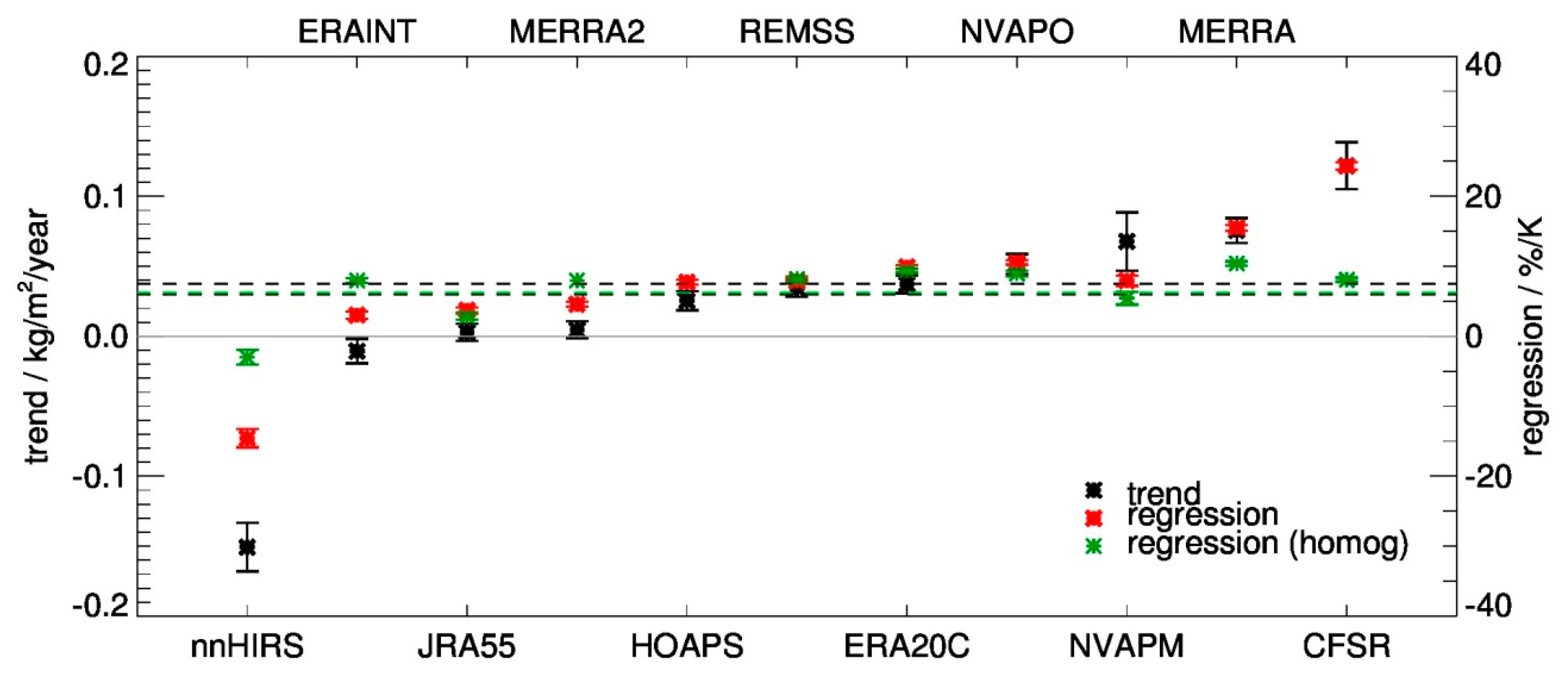
Figure 1 shows the trend estimates and regression coefficients over the global ice-free ocean within 60°N/S for each data record. The observed trend estimates range from −1.51 ± 0.17 kg/m²/decade (nnHIRS) to 1.22 ± 0.16 kg/m²/decade (CFSR) and exhibit large differences. Associated uncertainties are plotted as well and span values between 0.06 and 0.20 kg/m²/decade. In general, the trend estimates are significantly different among the data records. This is confirmed when tested following [7] and ignoring the covariance between trend estimates. Regression coefficients are also shown in order to assess the relationship between TCWV and SST changes as imposed by Clausius–Clapeyron. The minimum and maximum observed regression coefficients are −14.2 ± 1.3 %/K (nnHIRS) and 24.9 ± 0.5 %/K (CFSR), respectively, with 1.3%/K being the maximum uncertainty estimate. Again, the regression coefficients exhibit large differences among the data records. Furthermore, they are outside the expected theoretical range of 6.0%/K to 7.5%/K at 275 K imposed by Clausius–Clapeyron [30], with regression coefficients from HOAPS, the Merged Microwave REMSS, MERRA-2 and NVAP-M being close to the upper or lower boundary of this range. All regression values are significantly different from the expected value of 6.2 %/K, computed using the NOAA OI SST data record. It should be noted that a series of assumptions enter the regression analysis (see [7] for a discussion). In fact, dynamic processes like advection or large-scale circulation can lead to larger than expected regression coefficients with respect to Clausius–Clapeyron [31,32]. Also, it may be more appropriate to assess consistency with theoretical expectation using the SST during generation of the different data records. Previous studies also published trend estimates and regression values [11,30] and a summary on trend estimates in [33]. The summary in [33] exhibits a relatively large spread in trend estimates (−0.29 to 0.9 kg/m²). However, differences in temporal and spatial coverage and utilisation of different data record versions hamper comparability of results shown in [33] and between results found in the literature and published here. In summary, it can be concluded that based on the G-VAP data archive of long-term data records, the trend estimates are generally significantly different and are not in line with theoretical expectations.

In order to identify quality issues in the data records and to find explanations for the large differences in observed trend estimates, the degree of time series homogeneity, i.e., the presence of break points in the time series has been analysed over the global ice-free ocean within 60°N/S. The results for statistically significant break points from the PMF test are shown in

Table 2. Dates of observed break points, break sizes from the PMF test and coincident changes in the observing system or changes of the input to the assimilation schemes based on the analysis of TCWV anomaly differences relative to HOAPS for the global ice-free ocean within 60°N/S (extended and updated from [3,4]). Additionally, the break size from the SNH test is given when within a range of ±3 month of the date of the break point from the PMF test. Here, all given break sizes from the SNH test are significant. The break size is printed in bold when the results from both homogeneity tests agree on the date. The information on the various events is partly taken from figures published in the literature. Information on the status of NOAA satellites was received from http://www.ospo.noaa.gov/Operations/POES/decommissioned.html and https://poes.gsfc.nasa.gov/noaa-heritage.html.

Date yyyy-mm	Break Size kg/m2		Event
PMF	PMF	SNH
CFSR
1998-10	1.19	1.22	Approximate start of assimilation of NOAA15 data; approximate end of assimilation of NOAA11 and NOAA14 data; change from assimilating GOES09 to GOES10 data [20]
ERA-20C
2006-07	0.20	0.25	See text
ERA-Interim
1991-12	−0.58	−0.59	Approximate end of assimilation of F08 data and approximate start of assimilation of F10 data, approximate end of assimilation of NOAA10 data [22]
1994-11	−0.17	−0.06	Start of assimilation of NOAA14 beginning of 1995, approximate end of assimilation of NOAA11 data [22]
1997-04	−0.24	−0.18	Approximate change from assimilation of data from NOAA12 to NOAA11, see [22]
2000-05	−0.10		Approximate start of assimilation of F15 data and stop of assimilation of NOAA11 and NOAA15 data, see [22]
2006-06	0.20	0.34	Approximate end of assimilation of F15 and NOAA14 data, approximate change from GOES10 to GOES11, approximate start of assimilation of Meteosat 5 and 8 data, see [22], see text
2007-04	0.12		Approximate start of assimilation of Meteosat-9 data and approximate end of assimilation of NOAA16 data [22], note that the assimilation of Metop-A data started in late 2006/early 2007
JRA-55
2006-06	0.45	0.27	Start of assimilation of GNSS-RO refractivity observations in 2006-07 [23], see 2006-07 (ERA-Interim), see text
Merged Microwave REMSS
1993-04	0.11	0.09	See [4]
2006-07	0.16	0.17	See text and [4]
MERRA
1998-11	0.47	0.64	Start of assimilation of NOAA15 data in July 1998 [24] note: assimilation of AMSU-A and AMSU-B data (NOAA15) started on 1998-11-01 only while assimilation of HIRS data (NOAA15) started already on 1998-07-02 [34]
MERRA-2
1991-03	−0.46	−0.46	Start of assimilation of F10 data on 1990-12-09 [34]
1997-06	−0.21	−0.10	Start of assimilation of F14 data in 1997-05-08, of NOAA11 on 1997-07-15 and of GOES10 on 1997-04-25, end of assimilation of NOAA12 in 1997-05-23, increase in number of assimilated conventional data in early 1997 (aircraft mainly) [34]
2007-10	0.25		Start of assimilation of surface wind from WindSat in 2007-08, strong increase in number of assimilated AMVs from JMA and a decrease in number of assimilated AMVs from MODIS [25,34]
nnHIRS
1988-11	−0.58		NOAA11 declared operational on 1988-11-08
1991-12	−0.61	−0.99	NOAA10 on standby on 1991-09-17, NOAA12 declared operational on 1991-09-17
1993-02	−0.51	−0.25	See [4] for discussion on results related to NVAP-M. It seems that nnHIRS also exhibits increased uncertainties then.
1997-03	−0.96	−1.20	End of NOAA12 data on 1997-02-29
1998-05	0.35		Launch of NOAA15 on 1998-05-13
NVAP-M
1991-01	−1.18	−0.39	Launch of F10 in 1990-12
1991-11	1.67	1.12	Launch of F11 in 1991-12, stop of consideration of F08 data in 1991-12
1994-12	0.65	0.53	Approximate removal of NOAA11 from input, approximate start of consideration of NOAA14 data (see supplementary material to [26], also discussed in [26]
1998-10	−0.31		Approximate start of consideration of NOAA15 data (see supplementary material to [26])
2001-02	−0.53	−0.46	Approximate start of consideration of NOAA16 data (see supplementary material to [26])
NVAP-O
1991-03	−0.17	−0.09	Launch of F10 in 1990-12
1995-04	0.19	0.32	Launch of F13 in 1995-03

for all long-term TCWV data records of the G-VAP data archive. In the majority of cases (78%), the SNH test confirms the presence of break points detected by the PMF test. The break sizes estimated by both tests exhibit agreement and disagreement, with the maximum difference observed for the 1991-01 break point of NVAP-M. ERA-Interim exhibits the largest number of break points, six in total. This can partly be explained with the small variance of the associated anomaly difference (not shown) and its impact on the significance estimation. Break points larger than 1 kg/m² are observed for CFSR and NVAP-M. Table 2 further reveals that in the majority of cases the break points coincide with changes in the observing system or with changes in the input to assimilation schemes, with one exception (Merged Microwave REMSS in 1993-04) which was discussed in [4] and which has been confirmed by the SNH test. The discussion of the potential impact of the utilised reference [3] is updated here because more data records are considered: HOAPS anomalies are used as reference to compute anomaly differences. Thus, if HOAPS is affected by an inhomogeneity all data records should in principle exhibit this break point. ERA-20C exhibits a break point in July 2006. However, ERA-20C does not assimilate satellite data and therefore this break point might be caused by HOAPS. ERA-Interim, JRA-55 and Merged Microwave REMSS also exhibit this break point in July 2006 (i.e., in 40% of the cases) but not the other data records (CFSR, MERRA, MERRA-2, NVAP-M, NVAP-O and nnHIRS). In addition to the event for JRA-55 given in Table 2. this break point coincides with the activation of a radar beacon on F-15. After July 2006 HOAPS, ERA-Interim and REMSS are not considering data from F-15 anymore. Though a generally good agreement between results from the PMF and the SNH test is observed, discrepancies in the detection of break points and in the break sizes are present. These point to seeming shortcomings in the methods to detect break points and to the need to apply more than one test to approve or disapprove observed break points.

In order to assess the extent to which the observed break points contribute to the observed non-compliance with theoretical expectation imposed by Clausius–Clapeyron, the anomaly time series have been homogenised by successively shifting the anomaly time series with the information available on confirmed break points. Then, the regression coefficients have been recomputed and have been plotted in Figure 1. (green symbols). For five data records, the homogenisation leads to an improvement in the agreement with Clausius–Clapeyron. The regression coefficients for four other data records (ERA-20C, JRA-55, Merged Microwave REMSS, NVAP-O) are hardly affected while the regression coefficients for MERRA-2 change from values close to the lower limit of the expected range to the upper limit of the expected range. Though improvements are evident, i.e., the spread in regression coefficients is smaller and the coefficients are closer to the expected range (partly marginal though), non-compliance with theoretical expectation is still present, most obvious for nnHIRS. For nnHIRS, a decrease in anomalies is observed for the period 1988–1997. This decrease has been reduced by the homogenisation but is still evident in the homogenised anomaly time series (not shown). It can be concluded that homogeneity issues contribute to the non-compliance with theoretical expectation but seemingly additional issues and potentially also incorrectly detected break points lead to the non-compliance.

It can be concluded that the differences in trend estimates and the lack of compliance with theoretical expectation are at least partly caused by the presence of break points and that these break points coincide with changes in the observing system or in the input to assimilation schemes. Obviously, these break points are a function of data record. This is remarkable because all data records rely at least partly on SSM/I observations, except nnHIRS and ERA-20C. Only HOAPS and the Merged Microwave REMSS exhibit non-significant differences in trend estimates and agreement with theoretical expectation within uncertainty estimates.

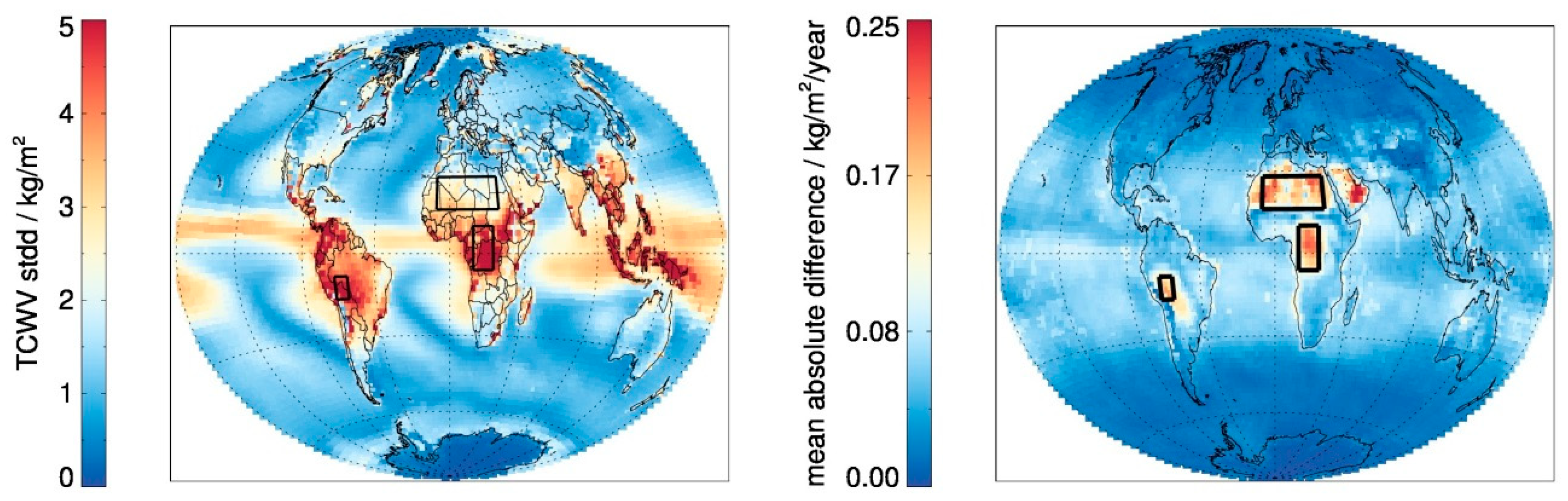
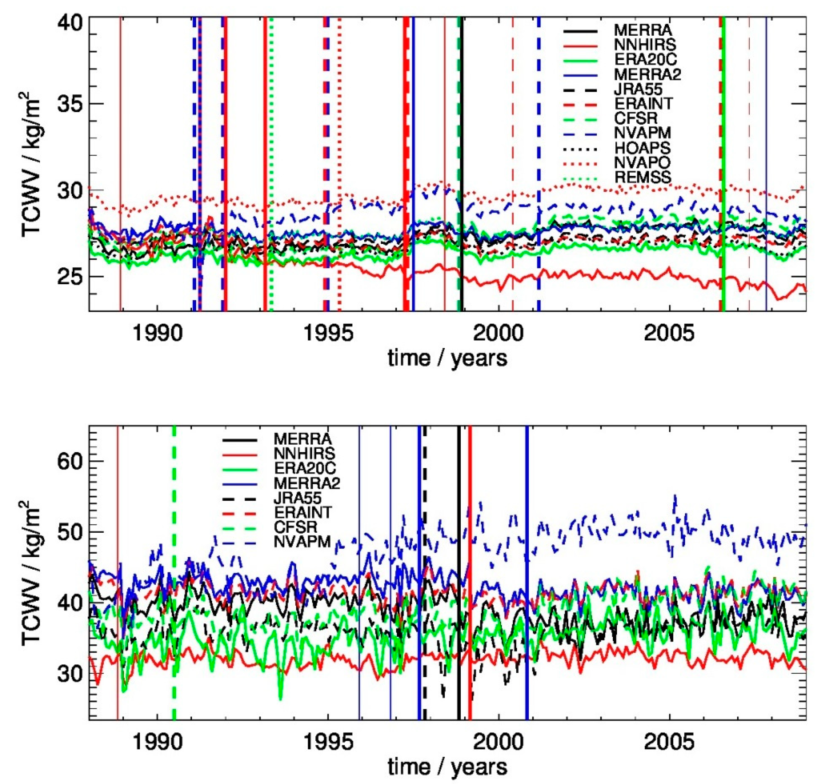
In global maps of the standard deviation and the mean absolute difference in trend estimates between the eleven data records (see Figure 2) distinct spatial features are observed over South America, central Africa and Sahara. Figure 3 shows time series of shifted TCWV anomalies averaged over the global ice-free oceans within 60°N/S and over central Africa. Also shown are the observed break points for both regions. Over central Africa, as for the global ice-free ocean, the break points coincide frequently with changes in the observing system (not shown). Note that it is unlikely that the reference data record ERA-Interim causes any of the observed break points over central Africa: only a single break point in summer 1997 is observed to occur in more than one case, here for MERRA-2 and JRA-55, and thus in less than 30% only. The spread in shifted TCWV anomalies over the global ice-free ocean is smallest in the early part of the common time period, i.e., from 1988 to 1995 and is generally large from 1999 onwards, with a maximum spread of 5.8 kg/m² (3.7%) in 2008. Generally, NVAP-O and nnHIRS exhibit maximum and minimum values, respectively. Obvious features include anomalies in 1997/1998, associated with the El Nino event and a decreasing trend in nnHIRS. The temporal evolution of the spread in shifted TCWV anomalies is similar over central Africa. However, the overall spread is larger with maximum values exceeding 20 kg/m² (50%) and the spread exceeds 10 kg/m² even in the early period. The reason for the spread being maximal in the 2000s is a single data record, i.e., NVAP-M. Obvious features are anomalies in JRA-55 in the late 1990s and an obvious break point in NVAP-M in 1995. Note that the break point in NVAP-M in 1995 has not been detected here but in [4] for reasons given in Section 2. In consequence, future homogeneity testing within G-VAP will include visual inspection of anomaly differences to identify obvious undetected break points. Remarkably, there is hardly any match between a confirmed break point for a specific data record in the top panel and in the bottom panel. This only occurs for MERRA (1998-11) and MERRA-2 (1997-06), i.e., in 12% of the 17 confirmed break points observed over the global ice-free ocean considering data records that include valid data over land and ocean. In a similar manner the number of coincident break points between the regions global ice-free ocean within 60°N/S, central Africa, Sahara and South America as marked in Figure 2. are analysed. For the six pairs of regions the maximum percentage of coincident confirmed break points is 12% which is observed for the pairs global ice-free ocean and central Africa as well as global-ice free ocean and Sahara.

In order to test the consistency of break points detected within a region and to confirm the regional dependency of break point detection, the following exemplary analysis has been carried out: The break point detection has been applied to three subregions of Sahara and the adjacent regions at the coast of west Africa and the Atlantic off the coast of west Africa (see figure in

Table 3. Dates of confirmed break points and break sizes from the PMF and the SNH test for the region Sahara and for five additional regions which are shown in the figure to the lower right. The results are based on the analysis of TCWV anomaly differences relative to ERA-Interim. Printed in bold and green are break points that are observed over Sahara and its three subregions and printed in italic and green are break points over the Atlantic which are different from the break points over Sahara. The figure is a zoom into the right panel of Figure 2. Marked in red is the region Sahara and marked in black are the five subregions: Sahara 1, Sahara 2, Sahara 3, Coast and Atlantic (from east to west). Each subregion has identical width and length in degrees latitude and longitude.

CFSR	Date yyyy-mm	Break size kg/m2		MERRA	Date yyyy-mm	Break size kg/m2
Region	PMF	PMF	SNH	Region	PMF	PMF	SNH
Sahara	2006-05	1.53	1.03	Sahara	2006-05	2.03	1.91
Sahara 1	---	---	---	Sahara 1	2000-11	1.50	0.53
Sahara 2	2006-05	1.71	1.32	Sahara 2	2006-05	2.37	2.37
Sahara 3	1998-03	−1.49	−0.98	Sahara 3	2006-05	1.95	1.36
Sahara 3	2006-05	1.43	1.22
Coast	---	---	---	Coast	---	---	---
Atlantic	1998-10	1.54	2.30	Atlantic	1991-12	0.96	0.83
					1999-01	0.75	0.13
NVAP-M	Date yyyy-mm	Break size kg/m2
Region	PMF	PMF	SNH
Sahara	1993-11	−7.62	−7.06
Sahara 1	1993-11	−7.52	−7.16
Sahara 2	1993-11	−7.31	−6.24
Sahara 3	1993-10	−7.83	−7.35
Coast	1993-09	−4.32	−4.17
Atlantic	2001-02	−1.81	−0.52

.). The region of Sahara has been chosen because it is the largest region considered and all data records that exhibit break points over Sahara have been analysed (i.e., CFSR, MERRA and NVAP-M). The results are shown in Table 3. Though the subregions over Sahara confirm the observed break points in 67% of the cases, sub-regional variability in break point detection is observed for CFSR and MERRA. All results over the Atlantic confirm the regional dependence of the break point detection, i.e., all detected break points occur at times different from those observed over the Sahara. Note that the dates of the break points over the Atlantic agree with the results over the global ice-free ocean shown in Table 2, except for the MERRA break point at 1991-12. Over the coast a mixture of land and ocean grids are analysed and no breaks are detected for CFSR and MERRA while for NVAP-M a break point at 1993-09 is observed, though with smaller break size than over Sahara.

The conclusion is that break points are not uniformly detected globally but are a function of region, confirming the results of [3]. This regional dependence was demonstrated for a few subregions here. It is assumed that the observed regional dependence of the break point detection is a function of the atmospheric and surface conditions that are prevailing in this region or of regional in situ or ground-based observations which are used as input. It needs to be emphasised that changes in the observing system might lead to inhomogeneities that are evident in specific regions only, and not in others. Thus, caution is needed when stability has been demonstrated using reference data with non-global coverage only. Reference [4] demonstrated that long-term continuous radiosonde data records are not available in regions with the observed distinct features. It was recommended to GRUAN to install a station over tropical land, e.g., in central Africa, dedicated to satellite evaluation in climate monitoring context.

5. Analysis of Gridded Water Vapour and Temperature Profiles

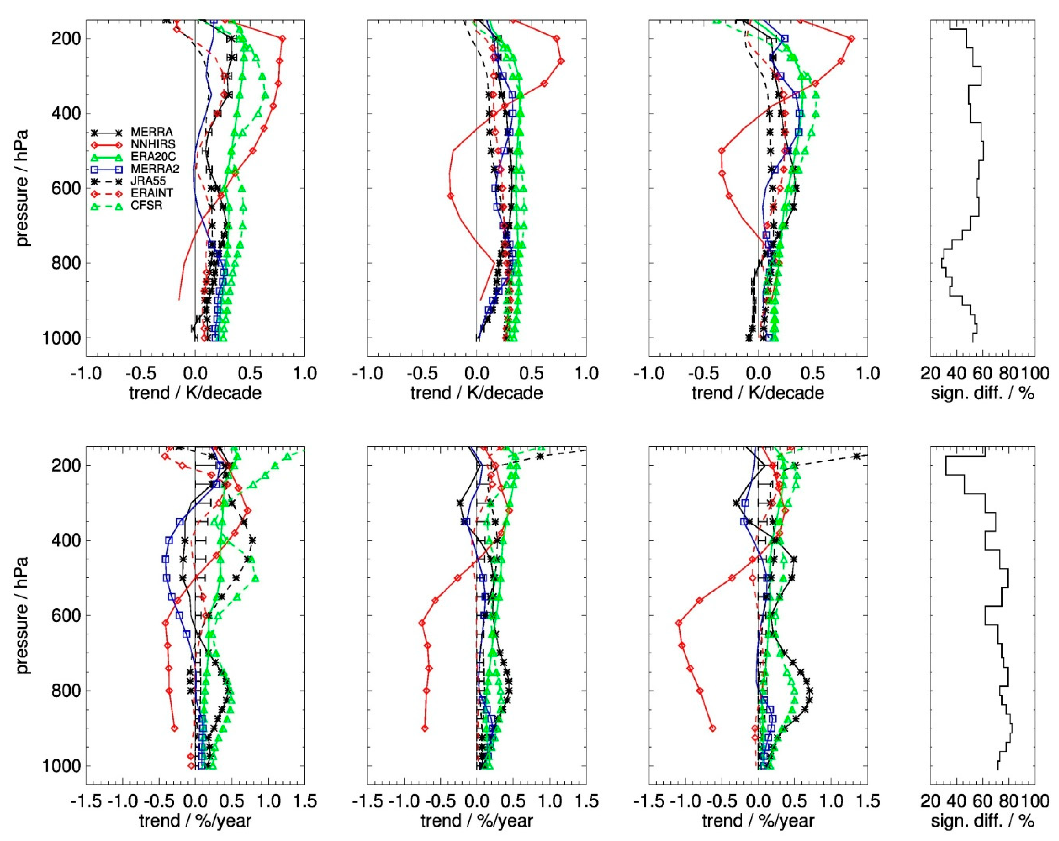
The assessment of water vapour and related temperature profiles focused on the analysis of long-term data records, i.e., with a temporal coverage of more than 20 years. Thus, the six reanalyses and the nnHIRS data records from the G-VAP data archive were analysed. Figure 4 shows profiles of q and T trend estimates for the tropics, the northern hemisphere and the southern hemisphere. The majority of trends in q are smaller than 0.5%/year while minimum and maximum values exceed ±1 %/year (CFSR, JRA-55 and nnHIRS). At near surface layers up to levels of approximately 900 hPa, the trends in q are generally small and exhibit a small spread. A first peak in the spread of trend estimates occurs around 800 hPa in all three latitude bands. Here CFSR and MERRA exhibit side maxima in trend estimates while the trends continue to be close to 0 %/year for ERA-20C, ERA-Interim, JRA-55 and MERRA-2 up to approximately 600 hPa. The trend estimates exhibit maximum spread in the upper troposphere in the tropics and a larger discrepancy in the southern hemisphere than in the northern hemisphere at all levels. Trend estimates for T profiles are usually smaller than 0.4 K/decade and do not exceed values of 0.9 K/decade. When nnHIRS is excluded maximum values hardly exceed 0.6 K/decade. Due to significant HIRS channel frequency changes in satellites operating in the 1990s nnHIRS (see also Table 2) appears as outlier in trend estimates of T and q. Generally, the T trend estimates are positive in all three latitude bands and at all levels. Also, the spread in trend estimates is small at near surface layers, starts to increase at levels around 700 hPa and is maximal in the upper troposphere in the tropics. As for q, the spread in T trend estimates is smallest in the northern hemisphere. Reference [10] also inter-compared vertical profiles of trend estimates and computed the regression between q and SST considering five data records of which one, namely MERRA, is also considered here. Though differences in temporal and partly in spatial coverage are present, their results also exhibit a side maximum around 800 hPa with comparable values for MERRA.

The degree of diversity in trend estimates among the data records is reflected in the percentage of data records being significantly different. This percentage was averaged over all three regions and is shown in the two right most panels of Figure 4. The most pronounced feature is the minimum in the upper troposphere for q. This is caused by the associated uncertainty of the trend estimate. For q, the relative uncertainty generally increases with decreasing pressure and exponentially reaches a maximum in the upper troposphere, inversely following the decrease of q with decreasing pressure, with values being an order of magnitude larger than at near surface layers. For T and q median percentage values are 51% and 73%, respectively. Thus, it can be concluded that the trend estimates in q and T are in the majority of cases significantly different.

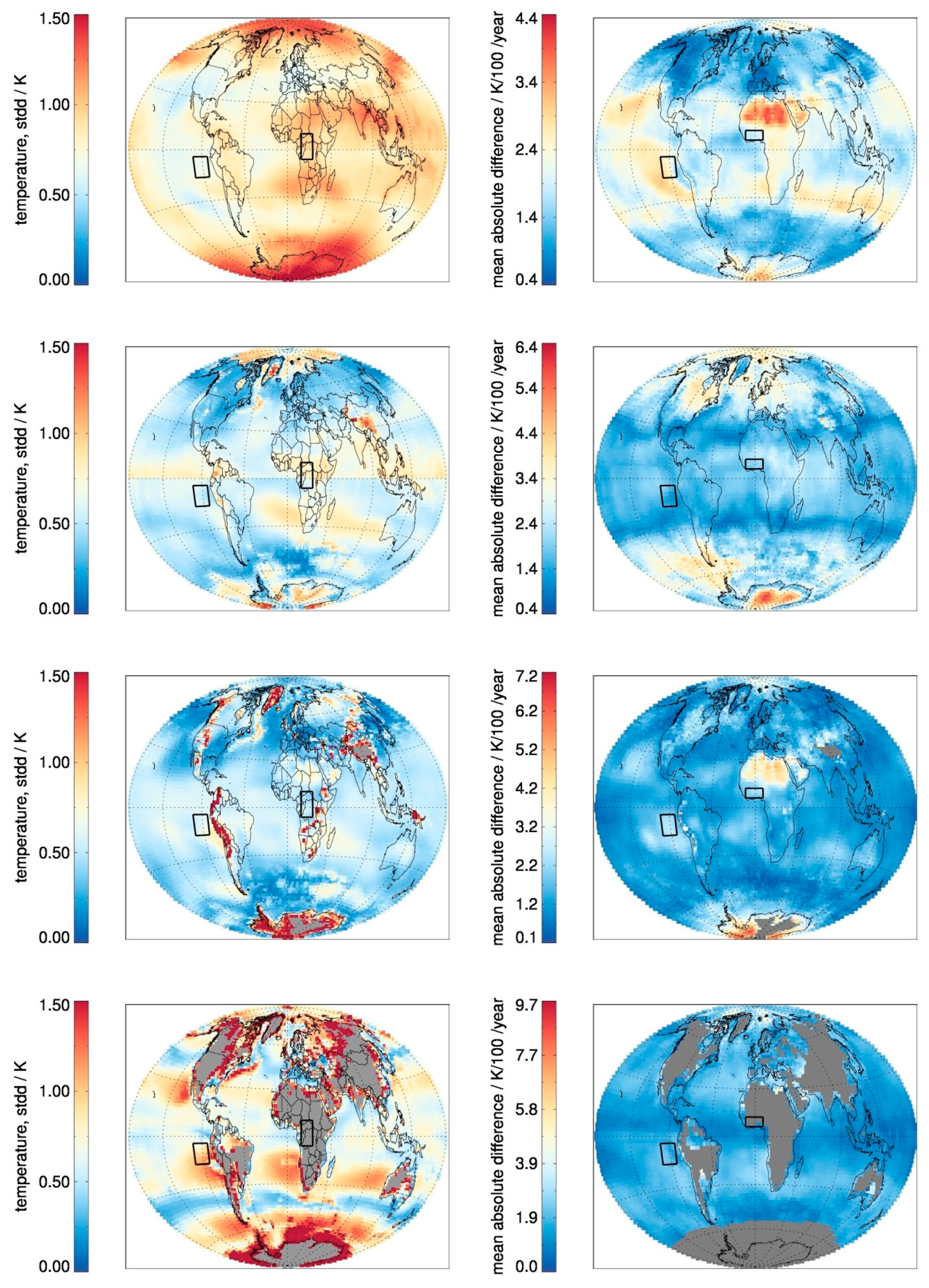
In order to showcase regional aspects of differences among the data records, Figure 5 and Figure 6 present global maps of standard deviations and mean absolute differences in trend estimates for the pressure levels 300, 500, 700 and 1000 hPa in relative and absolute units for q and T, respectively. Distinct regional features are found over stratocumulus regions (q at 700 hPa in left and right panels, q and T at 300 hPa in left and right panels, respectively), Antarctica (q at 300, 500 and 700 hPa in left panels, q at 300 hPa in right panel, T at all four levels in all panels, except at 1000 hPa in right panel), north pole (T at 300 hPa in left panel), central Africa (q at 300 and 500 hPa in left and right panels), Sahara (q and T at 700 hPa in right panels, T at 300 hPa in left and right panels) and over mountainous regions, in particular for T at 700 hPa. The relative standard deviation in q at 300 and 500 hPa exhibits values of >20% over large parts of the ITCZ and the warm pool. Also noticeable are standard deviations in T at 300 hPa which exceed 1 K over both poles and over large parts of northern and southern Africa, India and South-East Asia. Thus, large scale differences in q and T data records are observed in the upper troposphere. The retrieval of absolute humidity in the upper troposphere is a challenging task for the majority of observing systems [36,37], including radiosondes which are an anchor element during assimilation in reanalysis [22]. Thus, G-VAP will continue to analyse the quality of q and T profiles in the upper troposphere, among others, using the NOAA Products Validation System [38].

At 1000 hPa, maximum values in q and T are observed in the vicinity of undefined values. Differences in surface pressure between the data records contribute in two ways: first the difference itself will lead to differences in q and T and second it will impact the number of valid values. The latter point is supported by the right panels of Figure 5 and Figure 6 where data is excluded if 75% of the data is undefined. In case of the reanalysis, undefined values only occur if the surface pressure is smaller than 1000 hPa. Finally, note the spatial inhomogeneity at the equator in relative and absolute standard deviation in q and T at 500 hPa, respectively, and the distinct feature in T at 1000 hPa in the centre of the stratocumulus regions off the coasts of south-western Africa and South America. Both features vanish if nnHIRS is removed. The former feature can be explained with a hemisphere dependent training of the HIRS retrieval version used to build nnHIRS (a smoothing has been applied in newer versions since then, see [39]). Over Sc Pacific, nnHIRS exhibits the smallest temperature increase with the El Nino in 1997/1998 and exhibits a bias relative to the second largest difference relative to ERA-Interim thereafter (not shown).

Based on the inter-comparison results shown in Figure 5 and Figure 6 various distinct regions have been identified where further analyses is pursued. Here, the anomaly differences over Sc Pacific and western Africa have been analysed using the same approach as for TCWV. Statistically significant break points from the PMF test are summarized in

Table 4. Dates of observed break points, break sizes from the PMF test, and coincident changes in the observing system or changes of the input to the assimilation schemes based on the analysis of q and T anomaly differences relative to ERA-Interim for the region Sc Pacific (700 hPa) (extended and updated from [3]). Additionally, the break size from the SNH test is given when within a range of ±3 month of the date of the break point from the PMF test. Break sizes from the SNH test marked with an asterisk are not significant. The break size is printed in bold when the results from both homogeneity tests are significant.

Date yyyy-mm	Break Size g/kg		Break Size K		Data Record	Event
PMF	PMF	SNH	PMF	SNH
1988-10	−0.76				nnHIRS	NOAA11 declared operational on 1988-11-08
1991-08	0.53	0.08*			JRA-55	NOAA12 declared operational on 1991-09-17, approximate end of assimilation of NOAA10 data (MSU), see Figure 1 at http://www.remss.com/missions/amsu (JRA-55 utilizes MSU and AMSU data from REMSS [23])
1991-12	0.26	0.15			MERRA-2	Start of assimilation of F11 data in 1991-12-05, end of assimilation of F08 data in 1991-12-04 and of NOAA10 (MSU and HIRS) data on 1991-09-01 [34]
1997-03		0.21	−0.63	−0.25	CFSR	Approximate stop of assimilation of NOAA12 data [20]
1998-06	0.41	0.13			JRA-55	Approximate start of assimilation of NOAA15 data (Table A1 and Figure 4 of [23], approximate end of assimilation of NOAA12 (MSU), see Figure 1 at http://www.remss.com/missions/amsu
1998-10			0.85	0.52	CFSR	Approximate start of assimilation of NOAA15 data, change from assimilation of GOES09 to GOES10 data [20]
2001-03	−0.55	−0.73		0.89	MERRA	Start assimilation of NOAA16 on 2001-03-02 [24]
2001-04	−0.67	−0.22			CFSR	Approximate start of assimilation of NOAA16 data [20]
2003-08	−0.50	−0.16*			ERA-20C	See text

and

Table 5. As Table 4 but for the region western Africa (300 hPa) (extended and updated from [3]).

Date yyyy-mm	Break Size g/kg		Break Size K		Data Record	Event
PMF	PMF	SNH	PMF	SNH
1990-10			−0.38	−0.15	CFSR	Unclear, see text
1992-12			0.29	0.05*	MERRA-2	MSU channel 4 and SSU channel 3 exhibit anomalous behaviour around 1993-01 (see Figure 15 + 16 in [34]), sharp increase in upper air data assimilation from NOAA Profiler Network in 1992-05
1995-02	−0.03	−0.02			nnHIRS	NOAA14 declared operational on 1995-04-10
1997-03			−0.18		CFSR	Approximate stop of assimilation of NOAA12 data [20]
1998-09	0.05	0.02*		0.64	nnHIRS	Launch of NOAA15 on 1998-05-13, NOAA15 declared operational on 1998-12-15
2001-03			0.19		MERRA-2	Start assimilation of NOAA16 (HIRS) data in 2001-02-16, start assimilation of GOES IR data in 2001-04 [34]
2004-02			−0.16		MERRA	Abrupt decrease in number of assimilated ATOVS data in winter 2003/2004 [24], their Figure 4b), end of assimilation of NOAA16 data on 2004-05-20 in MERRA-2 [34], likely associated with an increase in noise level of HIRS data (see notice on 24 May 2004 at https://www.ospo.noaa.gov/Products/ppp/2004notices.html)

for the regions Sc Pacific and western Africa, respectively. Various break points have been observed for both regions, for both parameters and in particular for all data records. Maximum absolute values exceeding 0.75 g/kg and 0.5 K are observed for CFSR. As for TCWV, the observed break points coincide with changes in the observing system in the majority of cases. Note that no single break point occurred twice over western Africa and CFSR and MERRA, i.e., in 20% of the cases, have a common break point over Sc Pacific. This is an indication that ERA-Interim is not causing the observed break points. However, as ERA-20C is not assimilating satellite data, the break point observed in q over Sc Pacific in 2003-08 is either caused by the non-satellite input data or by ERA-Interim which was used to compute the anomaly differences. The latter is unlikely because such a break point is not observed in any other utilised data records. However, the observed break point approximately coincides with the end of assimilation of NOAA17 AMSU-A observations [22]. Finally, note that the anomaly difference between ERA-20C and ERA-Interim exhibits a decreasing trend for the period 2001–2005 (not shown). In the majority of cases (67%) the SNH test confirms the presence of break points detected by the PMF test over Sc Pacific while over western Africa only 29% of the break points from the PMF test are confirmed by results from the SNH test. Note that the break sizes estimated by both tests are different in the majority of cases. These results underline the previously made comment that the methods seem to have their shortcomings in break point detection and to the need to apply more than one break point test. The only exception from a coincidence of break point and change in observing system is the break point in T from CFSR in 1990-10 over western Africa. The SNH test detects a break point in T from CFSR over western Africa at 1990-07. Given the uncertainty of the break point detection this test confirms the presence of the break point. Though a break point in T at 300 hPa is concerned and though it is present in CFSR only it is mentioned for completeness here that this break point coincides with an abrupt decrease in number of TCWV data in ERA-Interim which have been assimilated under cloudy and rainy conditions [22]. The event for the 1992-12 break point in MERRA-2 is only indicative and was not detected by the SNH test. It can be concluded that numerous break points are present in q and T data records and that these break points lead to artificial trends. This will at least partly explain the spread in trend estimates. Reference [10] reached similar conclusions, which are confirmed and extended here via the application of a consistently applied approach to a comprehensive list of available q and T data records.

Interestingly, results shown in Table 4 and Table 5 do not exhibit a single match in confirmed break points between q and T. The break points in q and T have additionally been compared for the regions global (300, 700 hPa), Sc Pacific (700 hPa), western Africa (300 hPa), Sahara (700 hPa) and central Africa (300 hPa) (as marked in Figure 2, Figure 5 and Figure 6.). The maximum relative number of coincident confirmed break points between q and T is 11% and occurred over the region global (300 hPa). Thus, it can be concluded that the observed break points are not only a function of data record and region but also of parameter. The following hypotheses might explain this dependency: (1) differences in start or end of utilisation between data from different sensors of a specific satellite, and (2) retrieval or assimilation specific details. First, the information content of the sensors is to some extent parameter dependent, e.g., AMSU-A is primarily sensitive to temperature and AMSU-B to water vapour. When available and if specific for a single sensor, sensor information has been provided in Table 4 and Table 5. Unfortunately, a clear conclusion is hardly possible given the available information from the literature. Second, though the retrieval or assimilation schemes use data from a specific sensor as input, the data from that sensor might not pass quality control. The quality control largely depends on changes in the noise level of specific channels of the sensor and can cause anomalies and break points independently of the start and end of assimilation. The impact on number of assimilated data counts and its temporal evolution can be fairly large as shown in [24], their Figure 4. However, this information is either not available or the actual date of a specific anomaly or break point is difficult to deduce from, e.g., provided figures in the literature. In summary, a sound explanation of the observed dependence of the break points on parameter cannot be given.

Various break points have been observed and in the majority of cases these break points coincide with changes in the observing system or in the assimilation scheme. Despite this high frequency in coincidence, a physical explanation of the impact of a change in the observing system, its impact on the retrieval or assimilation scheme and of subsequent aggregation on the presence of break points is not given here. More analysis would require, e.g., denial experiments as, e.g., done by [24] which are beyond scope. Abrupt changes in the noise level or other sensor issues, changes in calibration which have not been accounted for, and the impact of quality control on number of input data can also impact the degree of homogeneity. To our knowledge, changes in the retrieval or assimilation schemes during processing did not occur. It would be advantageous to provide sensor specific information on number of actually considered data counts, in addition to start and end dates of general utilisation. Also, climate variability, e.g., associated with the Pinatubo eruption in 1991, the strong El Nino in 1997/1998 or the change from El Nino to La Nina in 1998, can impact the degree of homogeneity if the reference and the data record retrieval/assimilation schemes and/or sampling differences cause different responses to these events. Finally, uncertainties in the detection of break points are present. The reliability of break point detection decreases with a decrease in the ratio of break size and variability. Small regions can exhibit larger noise levels, so that a variable size of considered regions can impact the comparability of detected break points between these regions.

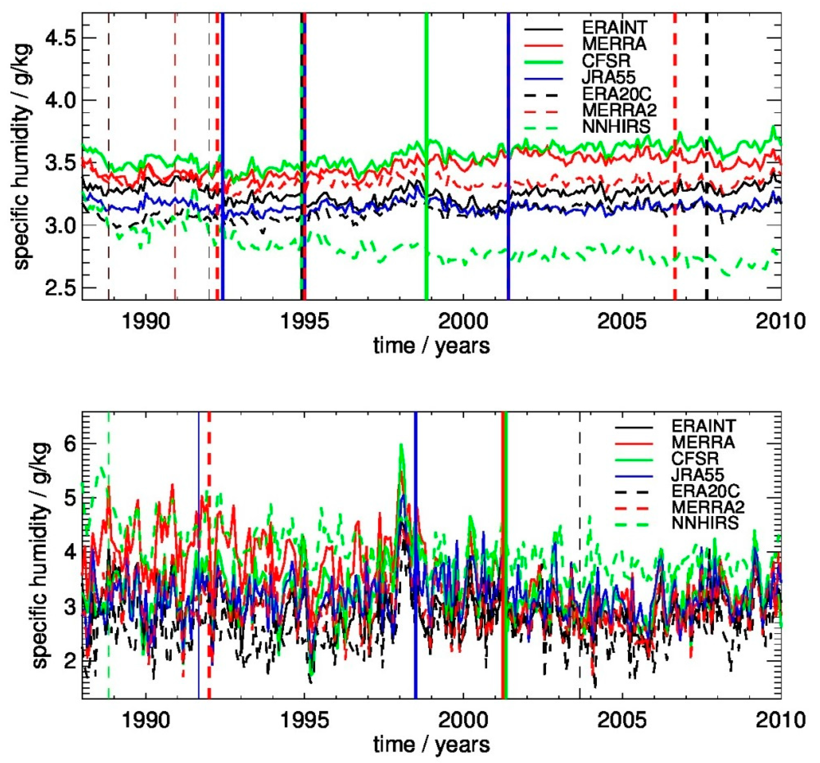
Figure 7 shows time series of anomalies of q averaged globally and over Sc Pacific. Also shown are the observed break points for both regions. Globally, the spread between the data records reaches generally larger values in the 2000s, with its maximum being 1.0 g/kg (28%) in 2009. nnHIRS exhibits a decreasing trend and minimum values while CFSR shows maximum values. Over Sc Pacific the maximum spread is observed in the 1990s and in the late 1980s, with a maximum value of 3.4 g/kg (25%) in 1988, and generally smaller values are present in the 2000s. ERA-20C and nnHIRS exhibit minimum and maximum values, respectively, and MERRA and nnHIRS also show decreasing trends. Prior to further analysis it was assessed if the reference ERA-Interim causes break points in the anomaly differences. The frequency of occurrence of break point detection exceeds 50% for a single case: 1994-11 for the global analysis. In this case, CFSR, ERA-20C, JRA-55 and MERRA-2 exhibit a break point and thus, it is concluded that ERA-Interim is likely causing this break point. In addition, ERA-20C exhibits four break points, one of them in 1994-11. All these break points coincide with changes in the satellite observing system and as ERA-20C does not assimilate satellite data the break points are likely caused by ERA-Interim. However, a visual inspection of the anomaly differences of all considered data records does not indicate that the break points observed for ERA-20C are evident and should have been detected, except for an anomaly in the early 90s (not shown). In consequence, future analysis within G-VAP will repeat the homogeneity analysis with a reference being independent from the satellite potentially causing breaks in the reference data record in case spurious breaks are observed. Hardly any match between a confirmed break point of a specific data record in the top panel and in the bottom panel is observed in Figure 7. This only occurs for MERRA-2 (1991-12), i.e., in approximately 9% of the cases (relative to the number of breaks in the top panel). This analysis is extended by determining the relative number of coincident confirmed break points between the regions global (300, 700 hPa), Sc Pacific (700 hPa), western Africa (300 hPa), Sahara (700 hPa) and central Africa (300 hPa) (as marked in Figure 2, Figure 5 and Figure 6), i.e., for each parameter 14 relative numbers have been determined. For q, the maximum relative number of coincident break points is 20% and occurs for the pair Sahara and central Africa at 700 hPa. In ten cases no coincident break points are observed. For T, 50% are determined for the pair western Africa and Sahara at 700 hPa. However, 0% relative coincidence occurs in nine cases and the average relative coincidence is 11% only. Thus, the conclusion for TCWV that break points are a function of region is also observed for q and T.

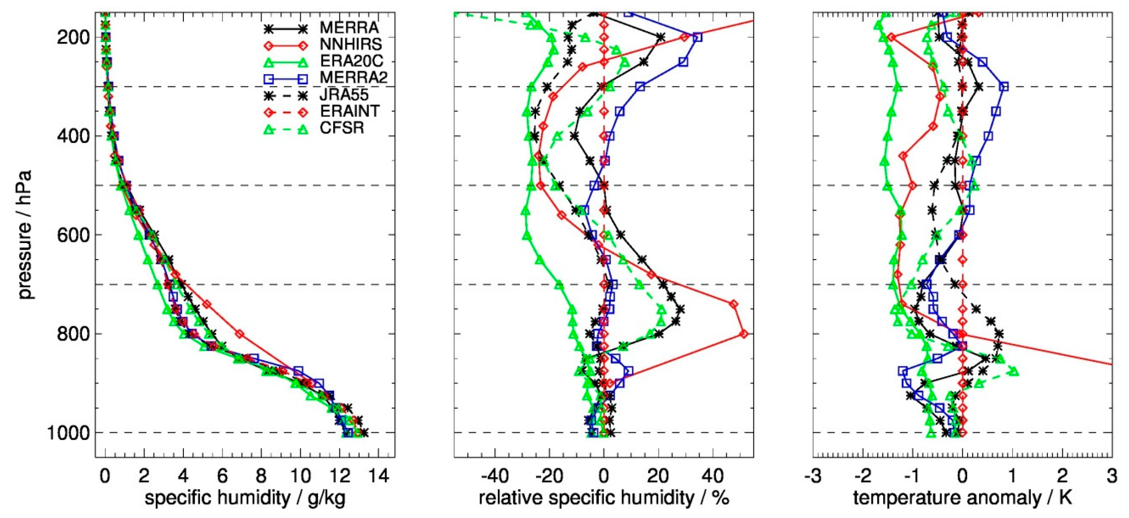
Profiles of q and T as well as q relative to data from ERA-Interim averaged over Sc Pacific marked in Figure 5 and Figure 6 are shown in Figure 8. At near surface layers average values are relatively close to each other. Starting at 900 hPa the spread among the data records increases. Distinct features are maximum spreads in q at 750 and 200 hPa and in T at 900–800 hPa and in the upper troposphere. Part of the spread around 800 hPa is obviously associated with differences in generally small values in the free troposphere and generally large values at the top of the planetary boundary layer. Note that the majority of data records are from reanalysis centres. Using radiosonde data from a field campaign in the East Pacific, in the vicinity of the box shown in Figure 5 and Figure 6, [40] showed that vertical profiles of specific humidity from ERA-Interim are too moist in the boundary layer, too dry in the free troposphere, have a too shallow boundary layer and an inversion which is not sharp enough (their Figure 5 and Figure 6). Our profile inter-comparisons exhibit similar features in overall profile shape with ERA-Interim being at the centre of the spread (middle panel of Figure 8). The authors of [40] further argued that the vertical distribution over stratocumulus regions is controlled by the model itself and not by observations.

In view of these fairly large differences observed in averaged profiles of q and T, their distinct regional features and with the presence of various break points it is recommended to conduct enhanced quality analysis of q and T profile data records over stratocumulus regions.

6. Discussion Based on Case Studies and Instantaneous Data

In addition to break points, various other factors impact the accuracy and precision of water vapour data records and observed differences between them. Ideally, all processes with impact on the data record’s accuracy and precision need to be fully understood, quantified and verified. Recently various efforts such as GRUAN, EUMETSAT CM SAF, CCI, the European Union projects FIDUCEO and GAIA-CLIM, the NASA Earth System Data Records Uncertainty Analysis Program and others have been conducted to assign uncertainties to in situ, ground-based and satellite data and to define a common language, appropriate metrics and best practices for validation (see [35,41,42,43,44]). The comprehensive description of sources of uncertainties, the propagation of uncertainties into higher level products via traceability chains, and the quantification of uncertainties for each value of the instantaneous and gridded products is challenging, requires substantial resources and becomes increasingly inquired. When available, the uncertainty estimates would improve our understanding of observed differences between data records and would need to be verified, i.e., consistency between the product and a reference, given respective uncertainties, needs to be demonstrated [45]. This requires quantitative information on uncertainties arising from collocation and on uncertainties of CDRs and reference data records. The latter two need to include propagated uncertainties from instantaneous data and uncertainties arising from spatial and temporal sampling. On basis of case studies, which were partly carried out in support to G-VAP, some of these uncertainty aspects are briefly discussed in this section.

For the consistency, analysis uncertainty estimates arising from collocation mismatches also need to be quantified. The collocation uncertainty might be negligible if the collocation window is small enough as, e.g., shown by [46]. Recently developed methods to explicitly estimate the collocation uncertainty are, e.g., the multiple triple collocation method described in [47] and the Observing System of Systems Simulator for Multi-mission Synergies Exploration using NWP fields [48] (see also [35]). References [49,50] analysed the collocation uncertainty as function of spatio-temporal mismatch for relative humidity and one conclusion is that the sensitivity of the root mean square difference to temporal mismatches reaches a maximum around 550–380 hPa with values around 1 %/hr.

The majority of satellite products of the G-VAP data archive are based on observations from polar-orbiting platforms and may therefore be affected by uncertainties caused by insufficient sampling of the diurnal cycle of water vapour. Reanalyses assimilate all-sky radiosonde data over land and satellite data mostly under clear-sky conditions (with recent advances to assimilate also cloudy-sky satellite data), both with differences in diurnal cycles, diurnal sampling and associated uncertainties. For satellite-based data records the uncertainty associated with differences in the diurnal sampling of TCWV is relatively small in case of MERIS observations [51]. Reference [52] shows that this conclusion is valid for other polar orbiting platforms as well and that on a global average scale the associated uncertainties do not exceed 0.1 kg/m² or 0.8%. It is noted that the diurnal sampling uncertainties can still be of relevance, if data records affected by diurnal sampling uncertainties and/or orbital drift are used to assess climate change.

Observed regional maxima in standard deviations and in trend estimate differences in TCWV, q and T occur in regions with large mean cloud amounts: stratocumulus regions, tropical land areas, warm pool and ITCZ (see Figure 2, Figure 5 and Figure 6, see also [2]). UV/VIS, NIR and IR-based water vapour data records rely on retrievals which have been predominantly applied under clear-sky conditions. In these cases, the so-called clear-sky bias substantially contributes to the overall uncertainty. This effect is in order of 10% for TCWV [53] and is mainly caused by the fact that the specific humidity within clouds is generally larger than in surrounding clear-sky areas. This was analysed using data from a single microwave imager. Due to the strong diurnal cycle of clouds, in particular in presence of convection, results in clear-sky biases are likely a function of overpass time and number of samples. Thus, differences among clear-sky data records are likely affected by how the diurnal cycle of the clear-sky bias is sampled. Consequently, G-VAP recommends that the sampling of the clear-sky bias as a function of orbit characteristics and of the diurnal cycle of clouds should be analysed to characterise the sampling bias of gridded products from polar orbiting satellites with UV/VIS, NIR and IR instruments on-board. Also, the removal of observations in presence of strong precipitation, as it is the case for several microwave-based water vapour products, might lead to an additional bias. If associated gaps are filled with data from surrounding (typically cloudy) areas, a systematic positive difference is introduced [54]. They noted that this systematic difference not necessarily reflects the true difference between rainy skies and cloudy skies. Recently, [28] estimated this bias at 15 GNSS stations to be on average −0.12 kg/m². They speculate that this bias might be larger in rainier cases. Consequently, it is recommended by G-VAP to characterise a potential bias between rainy-sky and cloudy-sky observations.

Also differences in the ability of the retrieval and assimilation schemes to retrieve extremes will impact the observed differences. In addition, the uncertainty characterisation typically relies on Gaussian statistics. However, water vapour distributions are typically non-Gaussian. For example, [55] analysed the PDF of q at 725 hPa over the tropics within a latitudinal band of ±30°N/S. The overall distribution is far from Gaussian and exhibits a pronounced maximum at small values, a saddle at intermediate values, a side maximum at large values and finally a tail towards maximum values. Considering the deconvolved GPS RO data from [56] as a reference, it became obvious that the utilised reanalysis data, NWP forecasts, other GPS RO data and profiles from hyperspectral sounders generally underestimate the peak at small values and the presence of extreme q values, i.e., the distribution fades at smaller values than the reference. Obviously a far more stringent quantification of differences is given by the analysis of the PDF instead of low order moments like mean and variance.

A prerequisite for the assessment of consistency is the availability of uncertainty estimates as an integral part of the satellite and reanalysis data records and in particular of the reference data records themselves. The efforts on assigning uncertainty and providing high quality reference data by networks such as GRUAN and by coordinated efforts such as GAIA-CLIM are cutting-edge, time consuming and challenging. It might be adequate to say that independent, fully characterized and traceable measurements have been successfully provided by GRUAN. Despite these efforts it seems that comparisons between GRUAN and satellite data, though meant to validate the satellite data, occasionally exhibit potential issues in the GRUAN data. E.g., [36] observe a bias between IASI and forward simulations of GRUAN day time observations which is outside the uncertainty range. Reference [42] summarised results from a workshop dedicated to inconsistencies among satellite data and reference observations, with similar conclusions. Reference [32] showed that the bias between IASI and GRUAN can be removed when adding 2.5 %RH to GRUAN data in the upper troposphere. At present GRUAN comprises 26 stations and 9 out of the 26 have been certified by GRUAN. Once fully established, GRUAN will likely encompass 30–40 stations. The GRUAN network expansion carefully considers satellite validation and climate monitoring requirements. However, certain areas of the Earth will remain to be underrepresented [57] and reprocessing activities of historical archives are not covered by GRUAN’s mandate. In order to further enhance the value of radiosonde data in the validation of satellite-based CDRs and to increase the number of collocations between satellite and radiosonde, G-VAP recommends to bias-correct and reprocess stable multi-station radiosonde archives of humidity and temperature going back to the 1970s (see also [33]). First steps in this direction were carried out by [58,59,60]. Efforts on the characterisation of satellite-based, ground-based and in-situ data carried out in different communities require feedback loops between all parties and are valuable to improve the (understanding of the) data and its quality. Such efforts are underway through developing GRUAN and Global Space-based Inter-Calibration System coordination to utilize GRUAN in satellite IR and microwave sensor assessments to verify uncertainty estimates.

G-VAP focuses on the analysis of gridded and temporally averaged long-term data records. The full characterization of uncertainties associated with instantaneous and gridded data records is not the objective of G-VAP. Instead, the goal of these case studies was to enhance our understanding of the uncertainty sources themselves, endeavoring towards an improved understanding of the differences observed among the various water vapour data records and an assessment of consistency. In view of the results of recent efforts on assigning uncertainties to ground-based, in situ, satellite and reanalysis data, it is recommended by G-VAP that activities on the validation of data records and within assessments need to make use of available uncertainty estimates to assess the degree of consistency.

7. Conclusions and Outlook

In order to characterise long-term water vapour data records from satellite observations and reanalysis G-VAP analysed results from (i) inter-comparisons, (ii) homogeneity tests and (iii) inter-comparisons of trend estimates on both global and regional scales. G-VAP started with an inventory of available water vapour and temperature data records and has provided a concise overview at http://gewex-vap.org/?page_id=13. Only data records with a minimum temporal coverage of ten years form the basis of the G-VAP data archive [2]. This archive includes 11 long-term and 22 short-term TCWV data records as well as seven long-term specific humidity and temperature data records on a common, regular longitude/latitude grid of 2° × 2°. The archive constitutes a valuable collection of data records for various applications such as inter-comparison studies, analysis of variability and climate model evaluation.

The G-VAP data archive formed the basis for the characterization of the quality of long-term water data records. The analysis of this archive led to various recommendations which have been summarised in

Table 6. Recommendations from G-VAP. More recommendations are given in [3].

Recommendation	Addressee
Need for improved recalibration and intercalibration of radiance and brightness temperature data records and homogeneous reprocessing of satellite data records	Space agencies
Provision and assessment of uncertainty estimates as an integral part of data records and reassess stability	Space agencies, PIs, G-VAP
Establish a station over tropical land	GCOS, GRUAN, GUAN
Need for development and sustained generation of a stable, bias corrected multi-station radiosonde archive including reprocessing of historical data	CGMS, WMO
Approach characterization of a potential bias between cloudy skies and rainy skies and of the clear-sky bias considering the diurnal cycle of clouds	Space agencies, PIs, G-VAP
Continue and refine quality analysis of profile data records over stratocumulus regions and in the upper troposphere	Space agencies, PIs, G-VAP

. Distinct spatial features in global maps of standard deviations and mean differences in trend estimates among the data records occur over central Africa, South America, Sahara, the poles and stratocumulus regions. Generally, reference in situ or ground-based measurements are not available in these regions. Thus, it is recommended that, e.g., in the process of extending GRUAN or of redefining GUAN, reference observations will become available in these regions. More generally speaking, a stable, bias corrected multi-station radiosonde archive needs to be developed and operated in a sustained environment including reprocessing of historical data.

Trend estimates were assessed on (near) global scale and for a number of regions. It can be concluded that these trend estimates are generally significantly different among the data records (TCWV, q and T) and are also typically outside the theoretically expected range dictated by Clausius–Clapeyron (TCWV). It was demonstrated that these inconsistencies are at least partly caused by break points which coincide with changes in the observing system in the majority of cases. These break points are a function of data record, region and parameter. In particular the regional imprint of changes in the observing system on stability in combination with the lack of reference observations with global coverage hampers the ability to demonstrate stability on global scale. These stability issues demonstrate the need to develop or improve quality control, recalibration and intercalibration of radiances and brightness temperatures, the data assimilation and bias correction schemes, and to frequently reprocess CDRs from satellite and reanalysis. The occurrence and strength of various break points have been documented here. In future efforts of G-VAP updated versions of the data records, ideally based on improved input data streams, will be analysed and the tabulated information on the break points will form a basis to assess the improvement in terms of homogeneity. Finally, it is concluded that the majority of widely used and well-established data records are affected by inhomogeneity issues and need to be utilised with great caution in climate analysis context. Despite these results, it should be noted that physical explanations for observed break points have not been provided and that the homogeneity tests exhibit not only agreement but also disagreement in break point detection.

It was consensus among G-VAP workshop participants to continue G-VAP beyond the finalisation of its first phase under the umbrella of GEWEX. It was agreed that G-VAP’s next phase will encompass continuity, e.g., quality analysis using PDFs and in the upper troposphere, an improved estimation of collocation uncertainties, and the assessment of improved stability of updated data records. Further, the homogeneity testing will be updated by visual inspection of anomaly differences and by utilisation of additional references. It will also include new activities which will partly be based on the G-VAP recommendations: It was decided to pursue the analysis of a potential bias between cloudy and rainy skies, to enhance the quality analysis of profile data records over the open ocean, in particular over stratocumulus regions and to characterise the clear-sky bias as function of the diurnal cycle of clouds. Finally, G-VAP supports the increasing demand for the provision of uncertainty estimates and will assess this uncertainty information in future activities.