Relative Altitude Estimation Using Omnidirectional Imaging and Holistic Descriptors


Departamento de Ingeniería de Sistemas y Automática, Miguel Hernández University, Avda. de la Universidad s/n, 03202 Elche (Alicante), Spain
*
Author to whom correspondence should be addressed.
†
These authors contributed equally to this work.
Remote Sens. 2019, 11(3), 323; https://0-doi-org.brum.beds.ac.uk/10.3390/rs11030323
Submission received: 27 December 2018
/
Revised: 2 February 2019
/
Accepted: 3 February 2019
/
Published: 6 February 2019
(This article belongs to the Section Remote Sensing Image Processing)
Abstract
:Currently, many tasks can be carried out using mobile robots. These robots must be able to estimate their position in the environment to plan their actions correctly. Omnidirectional vision sensors constitute a robust choice to solve this problem, since they provide the robot with complete information from the environment where it moves. The use of global appearance or holistic methods along with omnidirectional images constitutes a robust approach to estimate the robot position when its movement is restricted to the ground plane. However, in some applications, the robot changes its altitude with respect to this plane, and this altitude must be estimated. This work focuses on this problem. A method based on the use of holistic descriptors is proposed to estimate the relative altitude of the robot when it moves upwards or downwards. This descriptor is constructed from the Radon transform of omnidirectional images captured by a catadioptric vision system. To estimate the altitude, the descriptor of the image captured from the current position is compared with the descriptor of the reference image, previously built. The framework is based on the use of phase correlation to calculate relative orientation and a method based on the compression-expansion of the columns of the holistic descriptor to estimate relative height. Only an omnidirectional vision sensor and image processing techniques are used to solve these problems. This approach has been tested using different sets of images captured both indoors and outdoors under realistic working conditions. The experimental results prove the validity of the method even in the presence of noise or occlusions.

1. Introduction
Currently, the presence of mobile robots in our society has increased considerably. Initially, they were used to carry out some tasks that resulted in being very demanding or dangerous to human operators. However, at present, they are used in other countless tasks with different purposes, thanks to the evolution of the perception and computation equipment and techniques. Currently, they permit designing more autonomous robots that do not require human intervention to carry out their tasks. To fulfil their task, mobile robots must be able to plan a trajectory to arrive at the target points and navigate towards them while avoiding the obstacles in the environment. To accomplish the navigation task in an efficient way, it is necessary to carry out two fundamental tasks. On the one hand, an internal representation of the initially unknown environment (map) has to be created by the robot, and on the other, the robot must be able to estimate its position within this map. The robot needs one or more sensors to extract information from the environment in order to solve the mapping and localization problems. Several kinds of sensors can provide them with useful information, such as encoders, touch sensors, laser, or vision sensors. This information can be used both to build the model of the environment and to estimate the position of the robot.
Vision sensors have become one of the most widespread options in mobile robotics thanks to the big amount of information that they provide to the robot. Garcia et al. [1] presented a survey of mapping and localization methods using vision systems. They permitted different configurations, such as single cameras, stereo cameras, systems with an array of cameras, catadioptric systems, etc. Catadioptric vision systems consist of a single camera pointing to a convex mirror. This configuration permits taking images with a field of view of 360 degrees around the mirror axis. The richness of the information they capture is the reason why this kind of system has been chosen in this work. There are many previous works that have used catadioptric vision systems in navigation tasks. For example, Winters et al. [2] described a method for visual-based robot navigation using an omnidirectional camera. They demonstrated that it is possible to use this kind of image to perform localization tasks. Sometimes, the visual information is combined with other information sources such as encoders, GPS (Global Positioning System), or IMU (Inertial Measurement Unit). Oriolo et al. [3] presented a method for the localization of humanoid robots using a monocular camera, an IMU, encoders, and pressure sensors. Satici et al. [4] presented a navigation and control system for mobile robots that uses a vision sensor, an IMU, and an encoder. In the present work, the only sensor used to estimate relative altitude is a catadioptric vision system.
In recent years, some works have focused on the use of omnidirectional images as the only source of information to solve the mapping and localization tasks. For example, Caruso et al. [5] presented a method to perform visual odometry with a planetary rover using omnidirectional vision, and Corke et al. [6] developed large-scale SLAM (Simultaneous Localization and Mapping) using also omnidirectional cameras. The images contain much redundant information, which may change under many circumstances such as noise and occlusions. For this reason, it is necessary to extract some relevant information from each scene to create the map. This information must permit estimating the position of the robot with robustness. There are two different approaches to carry this out. On the one hand, the image can be described through the extraction and description of local landmarks from the scenes. As an example, Lowe et al. [7] carried out localization and mapping tasks using SIFT (Scale-Invariant Feature Transform), and Bay et al. [8] presented another interest point detector and descriptor, named SURF (Speeded-Up Robust Features). More recently, some alternatives have been presented to extract robust features from images captured with catadioptric vision systems and to match them [9,10,11]. The techniques based on local features can be considered mature methods, and some comparative analyses of their performance can be found in the literature [12]. On the other hand, more recently, a family of methods based on global appearance or holistic descriptors has emerged. They build one unique, compact descriptor per scene and usually lead to relatively straightforward mapping and localization algorithms, based on the pairwise comparison of descriptors. Payá et al. presented a study of the feasibility of some techniques based on the global appearance of omnidirectional images to carry out localization [13] and mapping tasks [14]. Fernández et al. [15] presented a global-appearance approach to carry out simultaneous localization and mapping tasks using hybrid metric-topological maps. The present paper makes use of holistic methods to describe omnidirectional images.
The map of the environment can be created using two main approaches: metrically or topologically. On the one hand, metric maps represent the environment defining the locations of some relevant characteristics with respect to a coordinate system. This configuration permits estimating the position of the robot with geometric accuracy. Munguía et al. [16] described a localization and mapping system, and they created the map using the metric information obtained by different sensors; an orientation sensor, a position sensor (GPS), and a monocular camera. Some other works used this metric approach in mapping and localization tasks, such as [17,18,19]. On the other hand, topological maps tend to model the environment as a graph with a set of nodes that correspond to different locations and the connectivity relationships between them. This mapping approach can be found in some works, such as [20], where a topological framework is used to carry out SLAM (Simultaneous Localization and Mapping) in an underwater environment using computer vision. More recently, some researchers have combined the metric and topological concepts to generate hybrid maps, where the information is arranged into several layers with different levels of detail. Kostavelis et al. [21] created different map layers using the concept of hybrid maps to carry out hierarchical navigation tasks. Dayoub et al. [22] presented a mapping and navigation system, which allows the mobile robot to plan paths and avoid obstacles using a topometric map composed of a globally-consistent pose-graph with a local 3D point cloud attached to each node. In the present work, the height estimation problem is addressed in a topological fashion.
The framework proposed in this paper is presented in the next lines. The robot operates in an environment using an omnidirectional vision system as the only source of information. We also consider that the map of the environment was constructed from a set of images captured while the robot had a planar movement and using global-appearance techniques. Previous works have shown that it is possible to estimate the pose (position and orientation) of the robot in this plane using this kind of technique [23]. In this work, Berenguer et al. used a set of omnidirectional images captured from different poses in the ground plane (reference images) and obtained a holistic descriptor per image, using a combination of the Radon transform and gist. These descriptors are used to build a local map of the environment, through a method based on a spring-mass-damper system, and the pose of the robot in the ground plane is subsequently estimated by comparing the holistic descriptor of the test image with the descriptors included in the map, through a distance measurement. Taking this fact into account, we propose to go one step further in the present work. The goal is to try to estimate, in addition to the in-plane position of the robot, the relative altitude where it is located without incorporating any additional information in the available map of the environment and using only the information captured by the omnidirectional vision system. In summary, the main objective of the paper is to propose a method based on the use of holistic descriptors to estimate relative height. The descriptors are obtained from the Radon transform of omnidirectional images, and the method consists of two main steps. First, the relative orientation between the reference and test images is calculated using POC (Phase-Only Correlation) [24] between the two Radon transform descriptors. Second, an approach based on a set of compressions and expansions of the columns of these descriptors is applied to estimate topological height. The method is able to estimate the altitude in outdoor and indoor environments with robustness against noise and occlusions.
The proposed method has been validated using different sets of images. First, it has been tested using our own synthetic set of images, captured using a virtual catadioptric vision sensor into two different synthetic rooms. This step was carried out with the objective of performing preliminary tests to improve the algorithm before considering actual images. Second, it has been tested using some sets of publicly-available actual images captured both indoors and outdoors, from a variety of positions. Additionally, a straightforward method based on the extraction and matching of local features is developed and run with comparative purposes, as a benchmarking method. It permits evaluating the relative performance (accuracy and computation time) of the method based on holistic descriptors, which is the main contribution of the paper. The remainder of this paper is structured as follows. Section 2 presents the state of the art of the altitude estimation in robotics. Section 3 introduces the method we use to describe global appearance, which is based on the Radon transform. Section 4 presents the algorithm we have designed for height estimation using holistic descriptors and the benchmarking method, based on local landmarks. Section 5 describes the publicly-available sets of images used to validate the approach. Section 6 presents the experiments and results. The last Section 7 outlines the conclusions.
2. State-of-the-Art on Altitude Estimation and Global Appearance Techniques
Recently, some developments have been carried out in the field of altitude estimation using vision sensors to solve the mapping and localization problems when the mobile robot can change its altitude during the operation, as in the case of UAVs (Unmanned Aerial Vehicles). Kim et al. [25] presented a vision system mounted in two different UAVs to assist the path planning of a ground vehicle, estimating its relative position and altitude. They used a single camera mounted on each UAV to capture the scenes. Others authors used a combination of sensors to carry out the altitude estimation task such as Angelino et al. [26], who combined the visual information of a monocular camera and the GPS to estimate the position and altitude of a high-altitude UAV. These works used a combination of several kinds of sensors or the use of two or more visual sensors to carry out the altitude estimation. Comparing to these works, the framework we propose uses only the omnidirectional images captured by one catadioptric vision sensor and global appearance methods (based on the Radon transform) to obtain a holistic descriptor per image and estimate the relative altitude of the robot.
The descriptors based on the global appearance of the scene gather information on the whole scene. Comparing to local methods, they do not extract any information on specific objects or landmarks. This characteristic can be an advantage because global appearance descriptors tend to be more compact, and less computational time is required to compute and compare them. Furthermore, they are a good alternative because global appearance descriptors represent the environment through high-level features that can be interpreted and handled easily. Furthermore, global appearance descriptors tend to be more robust against noise and partial occlusions in the images, compared to local descriptors, as shown in [27]. Several works have demonstrated the validity of these techniques in robot mapping and localization when the movement of the robot is restricted to the ground plane. For example, in [23], different 2D localization and mapping tasks have been carried out using global appearance descriptors, and they have been compared with some descriptors based on landmark extraction to compare the effectiveness and the computational cost. Ranganathan et al. [28] presented a probabilistic topological mapping method that uses information of panoramic scenes captured by a ring of cameras mounted on the robot, and they are described using Fourier signature. Furthermore, Menegatti et al. [29] showed a Monte Carlo localization method with omnidirectional images in large indoor environments using the Fourier signature as the appearance descriptor. However, few studies have been carried out about the altitude estimation using global appearance approaches. Bearing this view in mind, the objective of this work consists of exploring the use of a framework based on omnidirectional vision and global description to estimate the robot altitude.
The algorithm we propose estimates the relative altitude of the robot with respect to the altitude it had when the model was created, using only the visual information captured by the robot from its current position and the visual information stored in the model. There are many mobile robots that change their altitude during their operation, such as UAVs. Many previous works proposed different solutions to the localization problem using UAVs, such as [30], where these platforms were used in navigation tasks in outdoor environments using omnidirectional images and other different sensors such as gyro sensors. This work is mainly based on the detection of the skyline to calculate the altitude and the relative rotation of the robot. Ashutosh et al. [31] showed a combination of omnidirectional and perspective cameras to estimate the altitude of the UAV extracting some characteristics of the scenes.
Omnidirectional images are often transformed to panoramic before describing their visual appearance, such as in [32]. In the presented work, omnidirectional images are described directly, which supposes a reduction of the computational cost. With this aim, we make use of the Radon transform [33], which describes the image in terms of its line-integral projections along some sets of parallel lines. This type of descriptor has been used in [23] to solve the localization problem when the movement of the robot is restricted to the ground plane and has proven to be robust. In rough lines, the method consists of comparing the Radon transforms of two omnidirectional images captured from different altitudes. This comparison needs a previous step, which consists of calculating the difference between the two orientations the robot had when it captured the omnidirectional images. This step was carried out using POC (Phase-Only Correlation), proposed by Kuglin et al. [24]. A preliminary version of this method was presented in [34], where only virtual images were considered to evaluate its performance. In the present paper, the method has been improved, and a new distance measure has been included to work properly with images captured in real environments. The experiments include actual indoor and outdoor images. Additionally, a comparison with a method based on local features is included to prove the effectiveness of the proposed approach.
3. Describing the Global Appearance of Omnidirectional Images
This section presents the description method based on global appearance that we have implemented to describe the omnidirectional images. A comparison of description methods has been done in previous works [14].
To be useful in mapping and localization tasks, the descriptors should present several properties, such as a compression effect in the image information; a correspondence between the distance between two descriptors and the distance between the positions where the images were captured; a low computational cost to obtain and compare them; and robustness against changes in lighting conditions, noise, occlusions, etc. Furthermore, it should contain information on the orientation the robot had when it captured the image. We have chosen the Radon transform to describe the scenes. This mathematical transform has been used previously to describe images with the objective of solving 2D localization tasks [23], and it has been proven to meet all these properties.
The Radon transform was described initially in [33]. Previous research demonstrated the efficacy of this descriptor in shape description and segmentation such as [35,36]. Hoang et al. [35] presented a new shape descriptor, invariant to geometric transformations, based on the Radon, Fourier, and Mellin transforms, and Hasegawa et al. [36] described a shape descriptor combining the histogram of the Radon transform, the logarithmic-scale histogram, and the phase-only correlation.
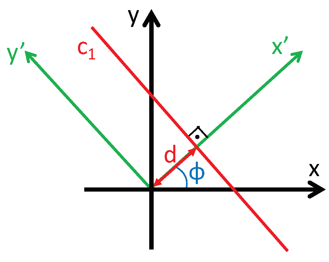
Mathematically, the Radon transform of an image along the line (Figure 1) can be obtained through the next expression:
where is the Radon transform operator. is the image to transform. is the transformed function, which depends on two new variables: the distance from the line to the origin d and the angle between the x axis and the axis, (Figure 1). The axis is parallel to the line.
By considering different values for d and in Equation (1), the transformed function will become a matrix with M rows and N columns. Normally, M is the set of orientations considered (to cover the whole circumference), and N is the number of parallel lines considered at each orientation (to cover the whole image). The distance between each pair of consecutive lines is considered constant.
This transform has been chosen to describe the scenes in this work because it presents some interesting properties. One of them is the scaling property, which is the basis of our altitude estimation algorithm: a scaling of the image by a factor in the x and y coordinates implies a scaling of the Radon transform: the d coordinate is scaled by a factor and the amplitude by a factor :
Another advantage is its robustness against noise or occlusions in the scenes, thanks to the integration process used to build the descriptor. This robustness against noise and occlusions is demonstrated in [23], in 2D localization, by comparing the Radon transform with other descriptors, both based on local features (SIFT) [7] and on global appearance (Fourier Signature (FS)) [37].
4. Altitude Estimation
This section details the altitude estimation method we propose, based on global appearance and the Radon transform (Section 4.1). Additionally, we have developed and implemented a method based on local features (Section 4.2) as a benchmarking method. Thanks to it, a comparative evaluation can be carried out to study the performance of the global appearance method with an approach based on the more classical extraction and description of landmarks.
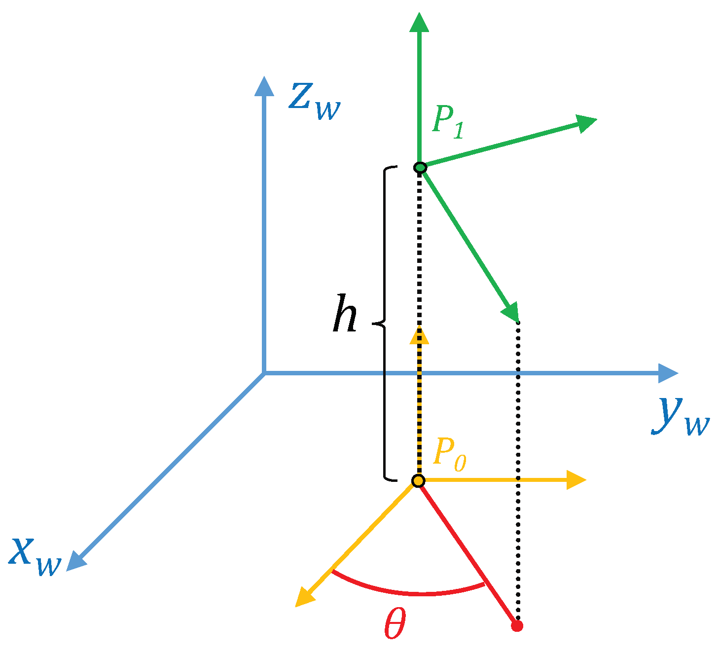
In both cases, the methods provide information on the magnitude and the direction of the vertical movement of the robot using only omnidirectional images captured by a camera mounted on the robot. To do this, the robot inclination with respect to the axis of the world reference system (Figure 2) must not change. Figure 2 shows the world reference system and the robot reference system. A change of the robot reference system is shown when it moves upwards from to . The method compares the images captured from and , and as a result, a topological estimation of the distance between these positions (relative altitude) is obtained.
4.1. Altitude Estimation Using an Approach Based on Global Appearance
In this subsection, the altitude estimation method based on global appearance is presented. First, the basis of the algorithm is described (Section 4.1.1). The method is based on the compression and expansion phenomenon that the Radon transform of omnidirectional images experiences when the robot moves upwards or downwards. Second, Section 4.1.2 presents the phase-only correlation, which is the method used to estimate relative orientation between two Radon transforms. Finally, Section 4.1.3 details the complete height estimation method, which is based on the two concepts presented in the two previous subsections.
The main steps of the method can be outlined as follows. First, the Radon transform descriptors of the reference and test images are calculated. Second, the relative orientation between these descriptors is detected and corrected. Third, a set of compressions, using some different compression factors, is applied to the columns of the descriptors. Fourth, the compression factors that produce the best match between the reference and test images are retained, and finally, the direction of the movement is detected. These steps will be explained in detail in the next subsections.
4.1.1. Compression-Expansion of the Radon Transform
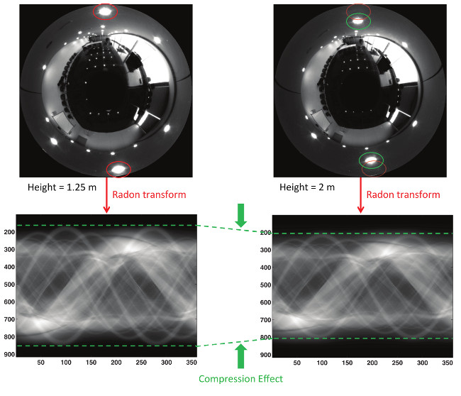
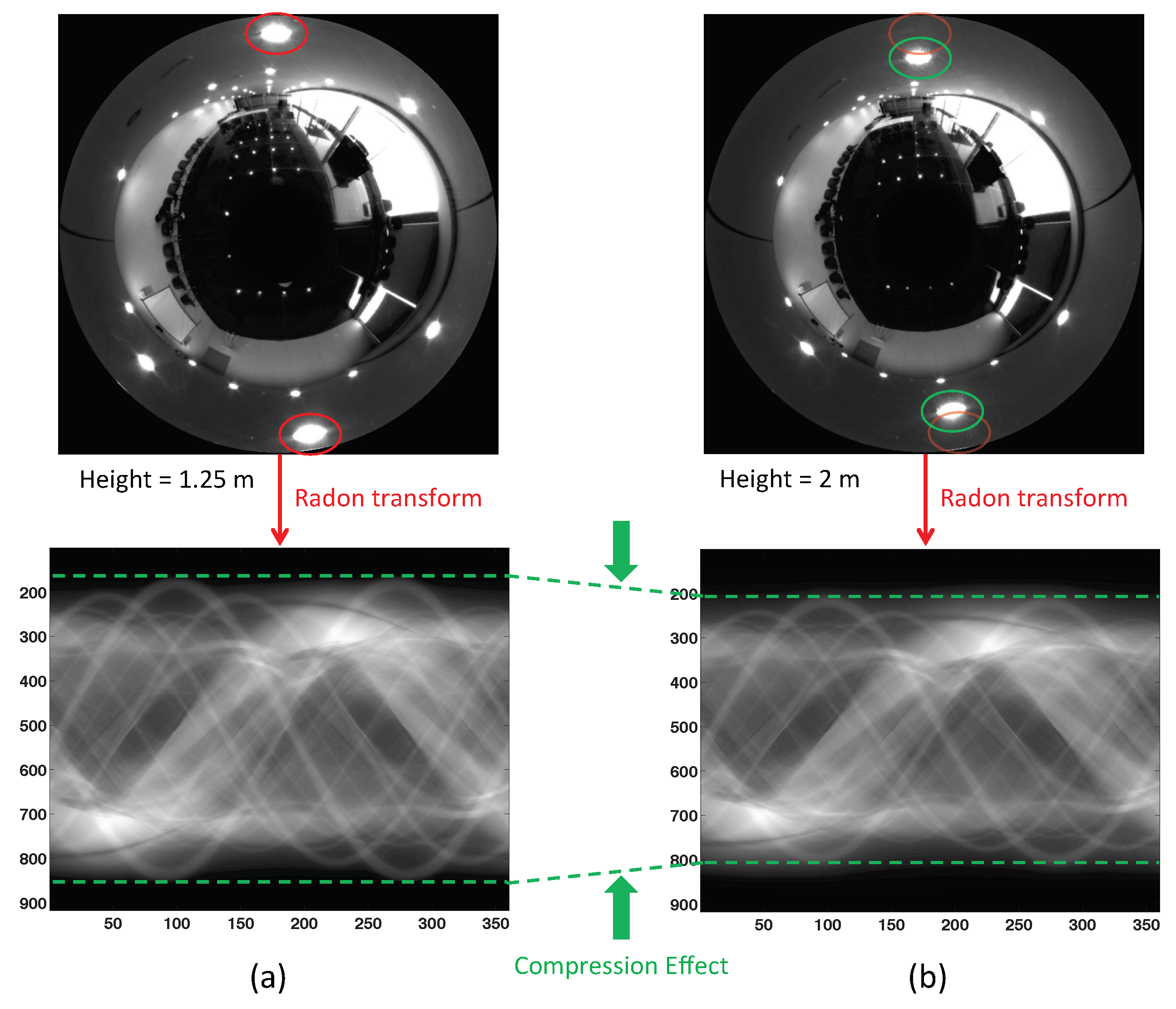
The method is based on the changes experienced by the Radon transform of two scenes captured from different heights when the robot moves along its vertical axis. If the vertical displacement is downwards, the objects in the omnidirectional scene tend to appear further away from the center of the image. This causes the information in the columns of the Radon transform to appear farther from the central row; vice-versa, if the displacement is upwards, the information in the columns tends to appear closer to the central row. This effect is related to the scaling property of the Radon transform.
The Radon transform undergoes a characteristic change owing to this property. The information in the columns of the Radon transform tends to move towards the central row (compression effect) when the robot moves upwards. However, when the robot moves downwards, the information in the columns tends to move away from the central row (expansion effect). This property is used by the method to estimate the relative altitude of the robot.
Figure 3 shows an example of this. Two omnidirectional images captured from different heights (1.25 m and 2 m respectively, with a purely vertical movement) and their corresponding Radon transforms are shown. In this figure, it is possible to observe that, in the second omnidirectional image, the objects have moved towards the center of the omnidirectional image compared to the first one. Both Radon transforms contain the same information, but the second one presents a “compression” effect with respect to the central row.
Therefore, it is necessary to design a procedure that permits quantifying these compressions/ expansions in the Radon transform and studying the correlation between these values and the altitude differences between the capture points of both omnidirectional images.
We consider that the robot has only moved along the axis, and the objective is estimating h (Figure 2). However, prior to this, it is necessary to detect if the robot has changed its orientation with respect to the axis, because it would introduce a shift in the columns of the Radon transform. This is a fundamental step to compare two different Radon transforms.
4.1.2. POC
In this subsection, we present the method we use to compare two Radon transforms. In general, it permits obtaining both the relative orientation between two different Radon transforms and a similitude coefficient between them, as shown in [23]. In the present work, POC is used only to estimate changes in the orientation of the robot around the axis. In short, a change of the robot orientation produces a shift of the columns of the Radon transform of an image, and POC is able to calculate it.
The POC operation between two matrices and with N rows and M columns can be calculated as:
where is the 2D discrete Fourier transform of and is the conjugate of the 2D discrete Fourier transform of . is the inverse 2D discrete Fourier transform operator. u, v are the variables in the frequency domain. is a matrix MxN of correlation coefficients that permits estimating the relative displacements between the two matrices along the axes x and y ( and , respectively) using Equation (4):
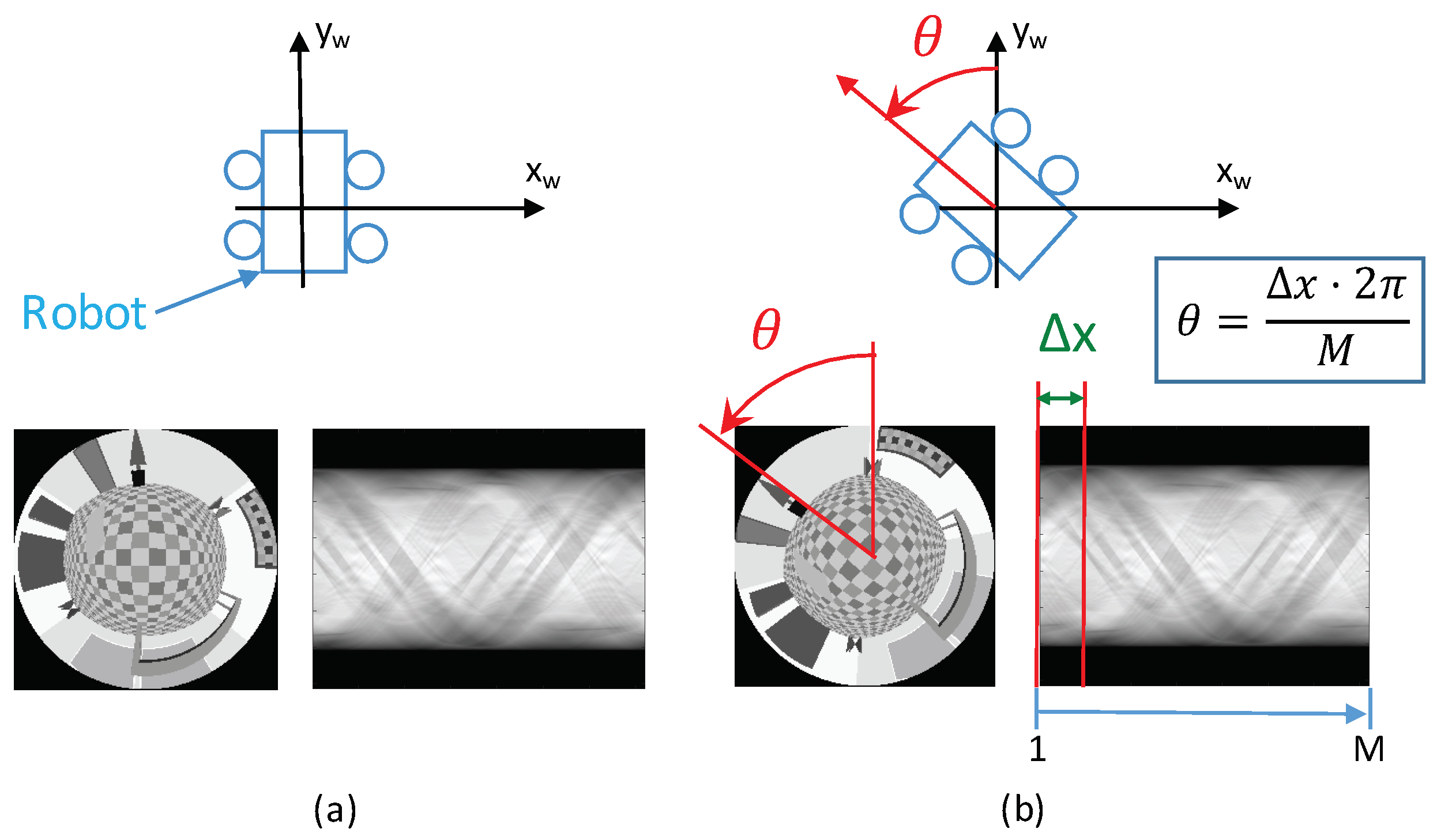
If we compare the Radon transforms of two omnidirectional images using POC, the value is proportional to the relative orientation of the robot when capturing the images according to Equation (5). Figure 4 shows the Radon transforms of two different omnidirectional images captured from the same point , but with different robot orientations with respect to the axis, .
This way, POC is able to compare two images independently of the orientation, and it is also able to estimate this change in orientation.
The POC operation compares two images based on their phase information in the frequency domain. This is an advantage with respect to other methods. Usually, only the magnitude is taken into account, and the phase information is usually discarded. However, when the magnitude and the phase features are examined in the Fourier domain, it follows that the phase features contain also important information because they reflect the characteristics of patterns in the images [38].
4.1.3. Height Estimation Method
The height estimation method is based on the concepts described in the two previous subsections. It is able to cope with changes in orientation with respect to the axis thanks to the use of POC to calculate this rotation using Equation (4). Figure 2 shows the world reference system () and the robot reference systems () when the robot is situated at the points and at with relative orientation with respect to .
The robot captures an omnidirectional image (reference image) from its initial position () and calculates its Radon transform. Then, the robot moves upwards or downwards, takes a new omnidirectional image (test image), and calculates its Radon transform. After this, the robot obtains the orientation change between both Radon transforms, using POC, and carries out the angular offset correction of the second Radon transform, by making a shift in columns equal to:
The next step consists of estimating the altitude difference between both images. Since a change of altitude produces a compression effect in the Radon transform with respect to its central row, the method applies a scale factor a to each column of the Radon transform of the test image, obtaining (the super-index indicates that the Radon transform has been compressed by a factor a using Equation (10)) and comparing the result with the Radon transform of the reference image (). This comparison is carried out using Equation (12), and the result is the distance between each pair of columns. This equation calculates a distance between and considering a normalization factor per column (they are normalized with respect to their maximum value).
The compression is carried out by interpolating the values of the Radon transform columns taking into account the scale factor a (expressed as the half of the difference between the number of pixels of the columns of both Radon transforms):
where is the number of pixels of the columns in .
where , , N is the size of the columns of the original Radon transform, and A is calculated using the following equation:
Furthermore, ⌊A⌋ is the largest integer less than or equal to A, and ⌈A⌉ is the smallest integer greater than A.
This step is repeated several times, considering different values for the compression factor , until the compression cannot be performed any more, because the compressed transform would not contain relevant information. At this moment, the robot has a vector of distance values calculated using Equation (12).
M is the number of rows of the Radon transforms, and N is the number of columns of . is the maximum value of the column j of , and is the maximum value of the column j of .
Each element of the vector has been calculated considering each magnitude of the compression factor .
From this vector, the compression factor that produces the minimum of the vector of distances (Equation (15)) can be considered as a magnitude that is proportional to the relative height.
At this point, it is necessary to distinguish if the translation of the robot has been upwards or downwards. The Radon transform of the test image experiences a compression effect when the translation is upwards. However, when the movement is downwards, the Radon transform of the reference image is the one undergoing the compression effect.
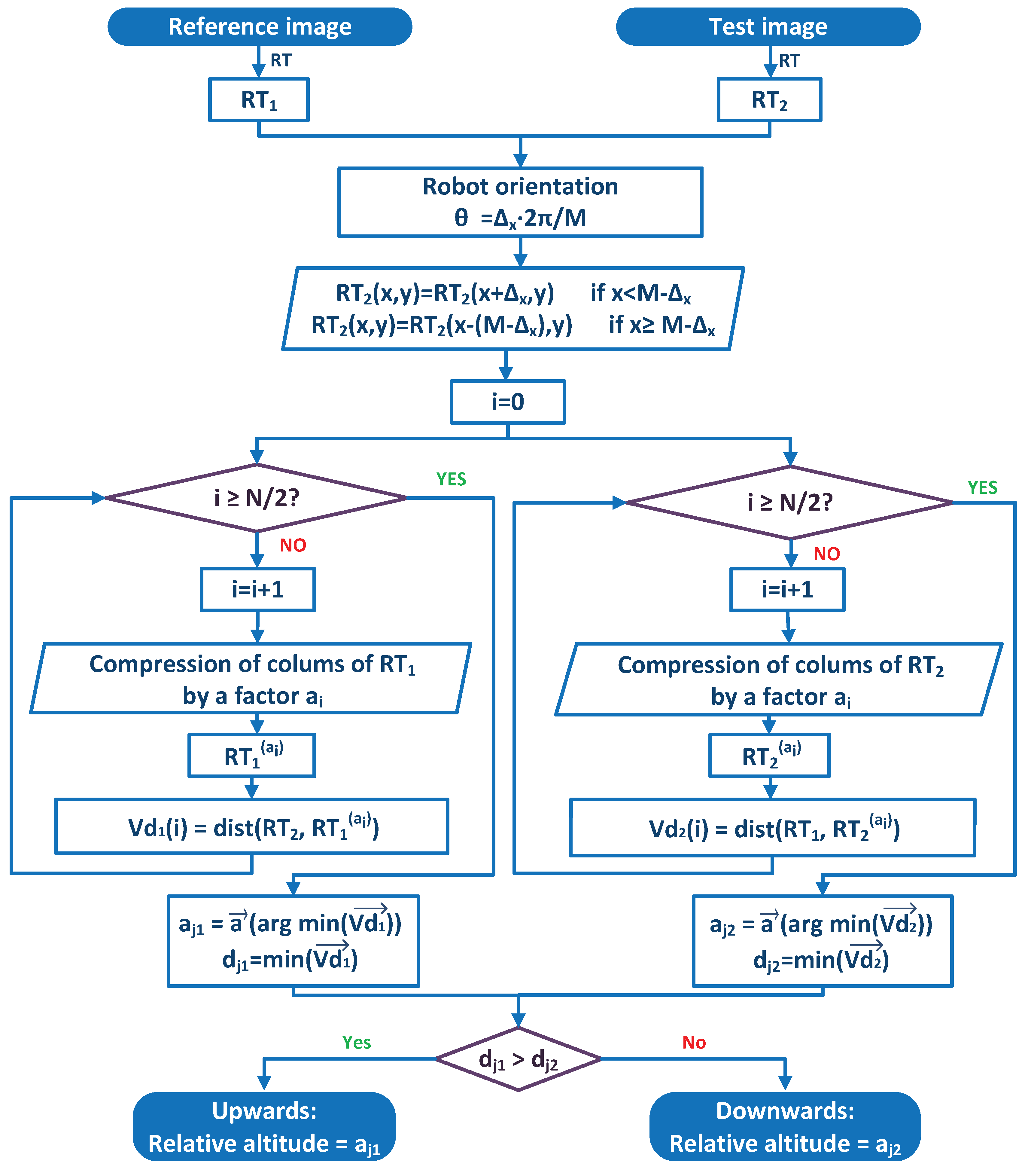
To distinguish the kind of translation (upwards or downwards), first, the Radon transform of the test image is compressed gradually, and the robot carries out the method described in the foregoing paragraphs, to obtain the factor, but in this case, the robot also has to save the minimum magnitude in the vector of distances . This case would be the correct one if the robot had moved upwards. Second, is compressed instead of , obtaining . This case would be the correct case if the robot had moved downwards. Finally, the robot has two factors: from the first case and from the second case, and it has two distances: (from the vector of distances of Case 1 (), Equation (16)) and (from the vector of distances of Case 2 (), Equation (17)). The minimum between and determines which is the correct case, Equation (18). At the end of the process, the robot has a magnitude proportional to the vertical displacement, and depending on the correct case, the displacement has been upwards (Case 1) or downwards (Case 2). Figure 5 shows a complete flowchart of this process.
4.2. Altitude Estimation Using an Approach Based on Local Features
In this subsection, an alternative method based on local features is proposed, with the objective of having a benchmarking method to compare the performance of our global appearance approach. The next paragraphs describe the steps of this method.
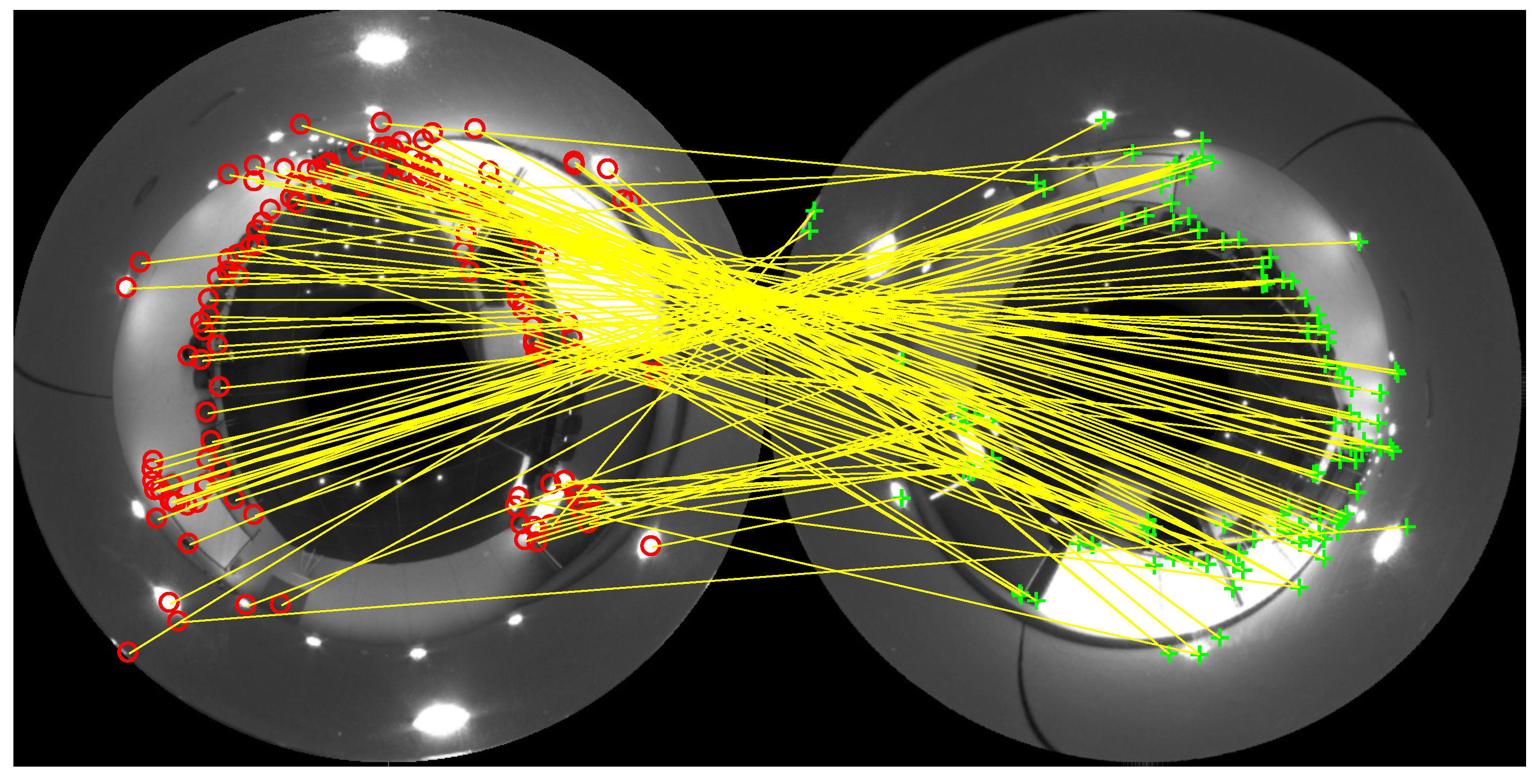
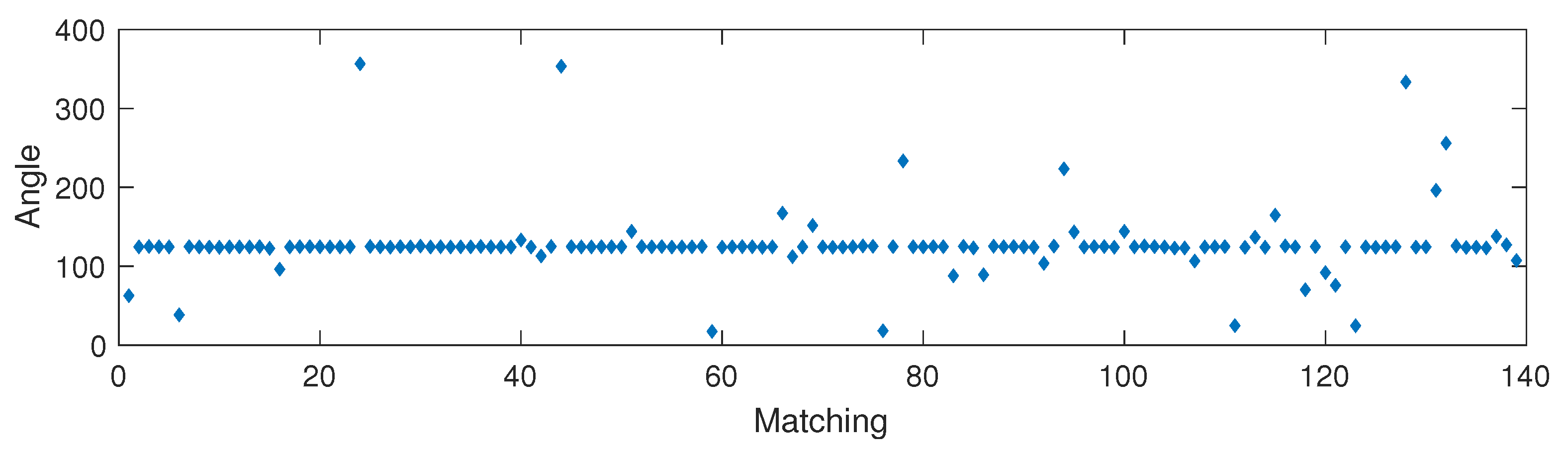
The robot takes an image (reference image) from its current position. Then, it moves upwards or downwards and takes another omnidirectional image (test image). The local landmarks of each image are calculated using any landmark detection algorithm. At this point, the robot has the two images with the landmarks in each image, so it needs to do the matching between the landmarks in the reference image and the landmarks in the test image (Figure 6). Then, the robot has to determine the rotation difference between both images (rotation around the axis). If there is not a rotation, each matching will have a direction that would be the same direction as the one between the landmark of the first image and the center of the image. If it is not the truth, there is a rotation. To estimate it, the angular difference between both directions is calculated for each pair of matched landmarks. Then, all differences calculated are compared using RANSAC (Random Sample Consensus) to get the most repeated difference value (Figure 7). This value is the rotation difference between both images, and the matches with a different value of orientation (outliers) are discarded. Then, the second image is rotated by this angular difference, and the relative altitude estimation is carried out calculating the mean of the distance between all new matched landmarks.
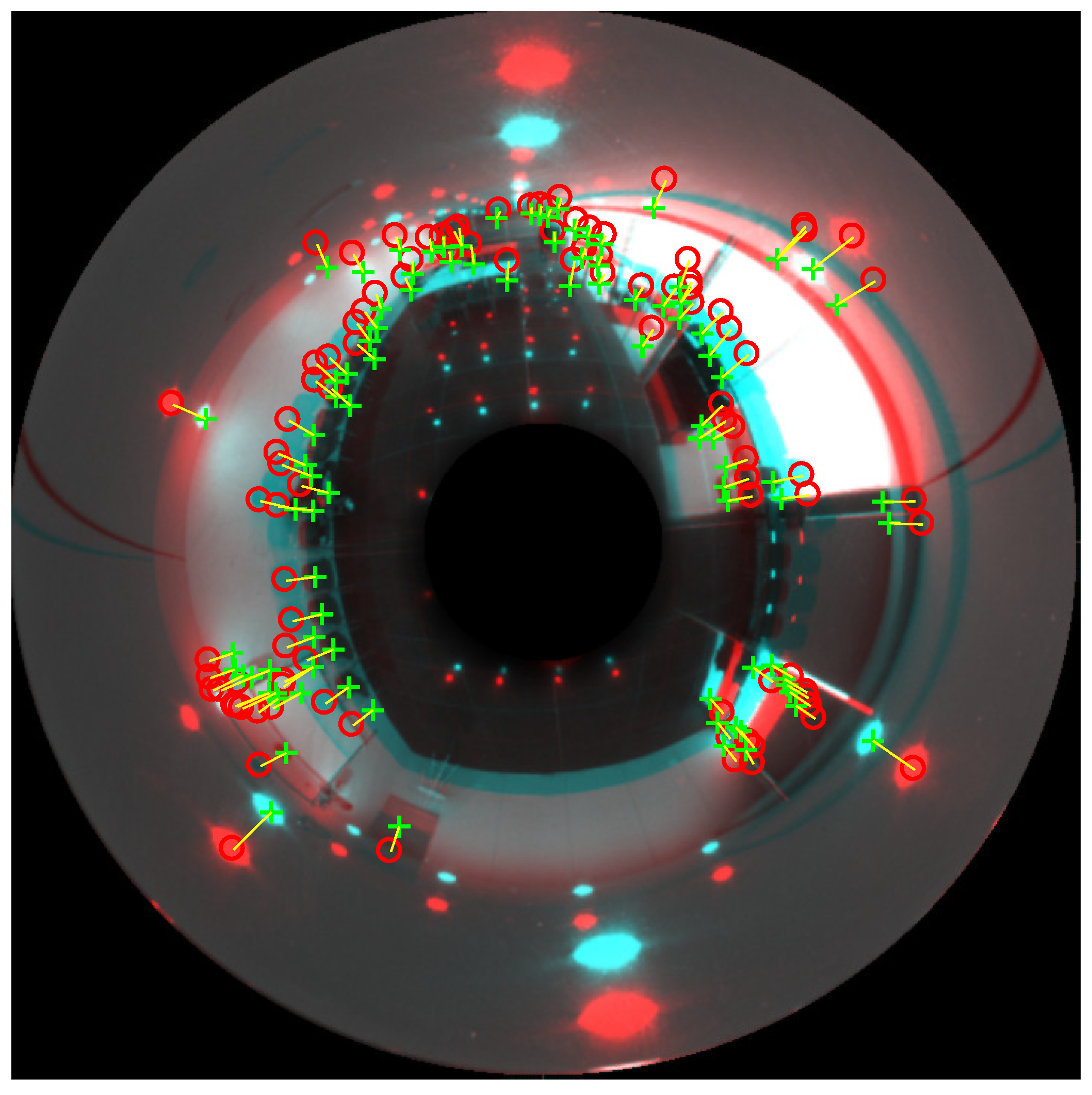
Figure 8 shows an example of two omnidirectional images compared to calculate the distance between the matched features, to obtain the difference of altitude between them. The relative orientation has already been corrected, so all directions between matched landmarks are towards the center of the image. For the sake of clarity, the reference and test images are shown superimposed. The red colored image is the reference image, and the green colored is the test image. The red circles are the final landmarks in the reference image (once outliers have been removed), and the green crosses are the final landmarks in the test image.
While implementing this benchmarking method, two different algorithms have been considered to perform the extraction, description, and matching of landmarks. First, SURF (Speeded-Up Robust Features) points [8] have been considered, since it constitutes a classical framework in robot localization tasks. Second, ASIFT (Affine Scale-Invariant Feature Transform) features [10] have been used, because this method permits extracting and matching features that have undergone large affine distortions; hence, they may constitute a more robust option when working with catadioptric cameras.
5. Image Database
In order to test the performance of the proposed technique, different sets of omnidirectional images have been considered. First, two virtual environments have been created to take omnidirectional images easily. These images permit testing the validity of the method under ideal conditions. After that, several sets of real images were captured both indoors and outdoors under real working conditions, and the algorithm was tested exhaustively with these actual images.
In the next subsection, the main features of both sets of images are outlined.
5.1. Set of Virtual Images
Two different virtual environments have been created, which represent two different rooms. These virtual environments permit creating omnidirectional images from any position and with any orientation. The algorithm to create these virtual images is described in [23].
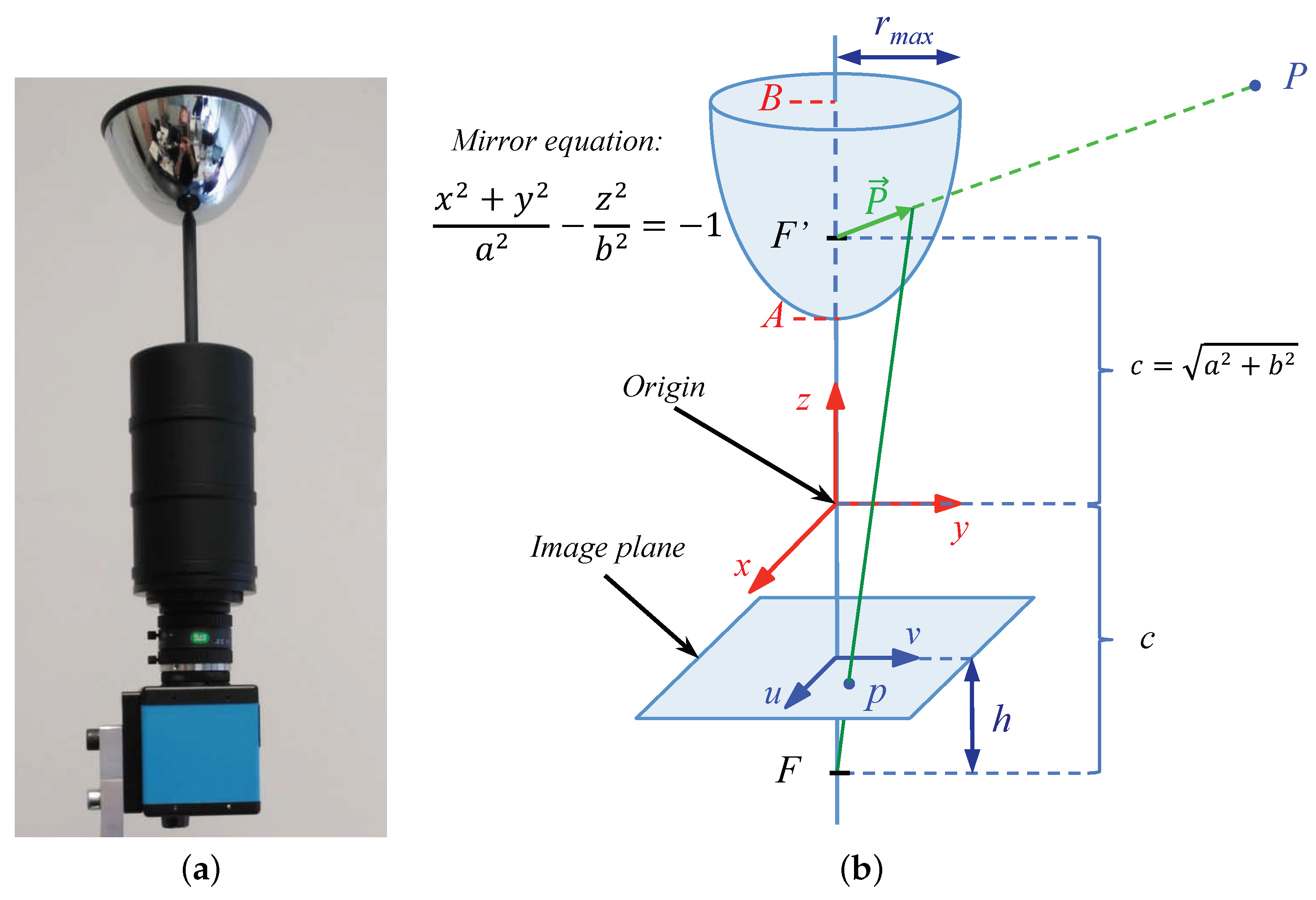
The omnidirectional images used in the experiments have pixels. These images have been created simulating the hyperbolic mirror described in Figure 9b. The parameters used in the mirror equation are mm and mm.
To generate the virtual database, several images have been captured in both environments. Several positions have been chosen on the floor of each environment, and a set of images vertically above these positions was captured to carry out the experiments. The maximum height is 2000 mm, and the minimum 100 mm, with a step of 100 mm. Therefore, this database permits testing the algorithm with a maximum change of height equal to 1900 mm between the reference and test images. Two samples of omnidirectional images captured in one of these virtual environments are shown in Figure 4.
5.2. Set of Actual Images
In the previous subsection, a virtual images database has been presented. This database is used to make a preliminary test of the performance of the proposed technique. However, to test the effectiveness and the robustness of the method, it is necessary to use an actual database.
This actual database is composed of different omnidirectional images taken in different indoor and outdoor environments. These images have pixels. To create this database, 10 different indoor environments and 10 different outdoor environments have been used. In each environment, several images have been captured from a variety of altitudes. The minimum height in indoor environments is 1250 mm (h = 1), and the maximum height is 2300 mm (h = 8), with steps of 150 mm. In the outdoor environments, the minimum height is 1250 mm (named as h = 1 in the experiments) and the maximum height is 2900 mm (h = 12), with steps of 150 mm. Hence, the outdoor dataset permits testing the algorithms with a maximum change of height equal to 1650 mm between the reference and test images.
These omnidirectional images have been captured using the system shown in Figure 9a. This system is composed of a hyperbolic mirror, a camera, and a tripod to change the height. The coordinates of the capture point in each environment are the same; only the coordinate changes.
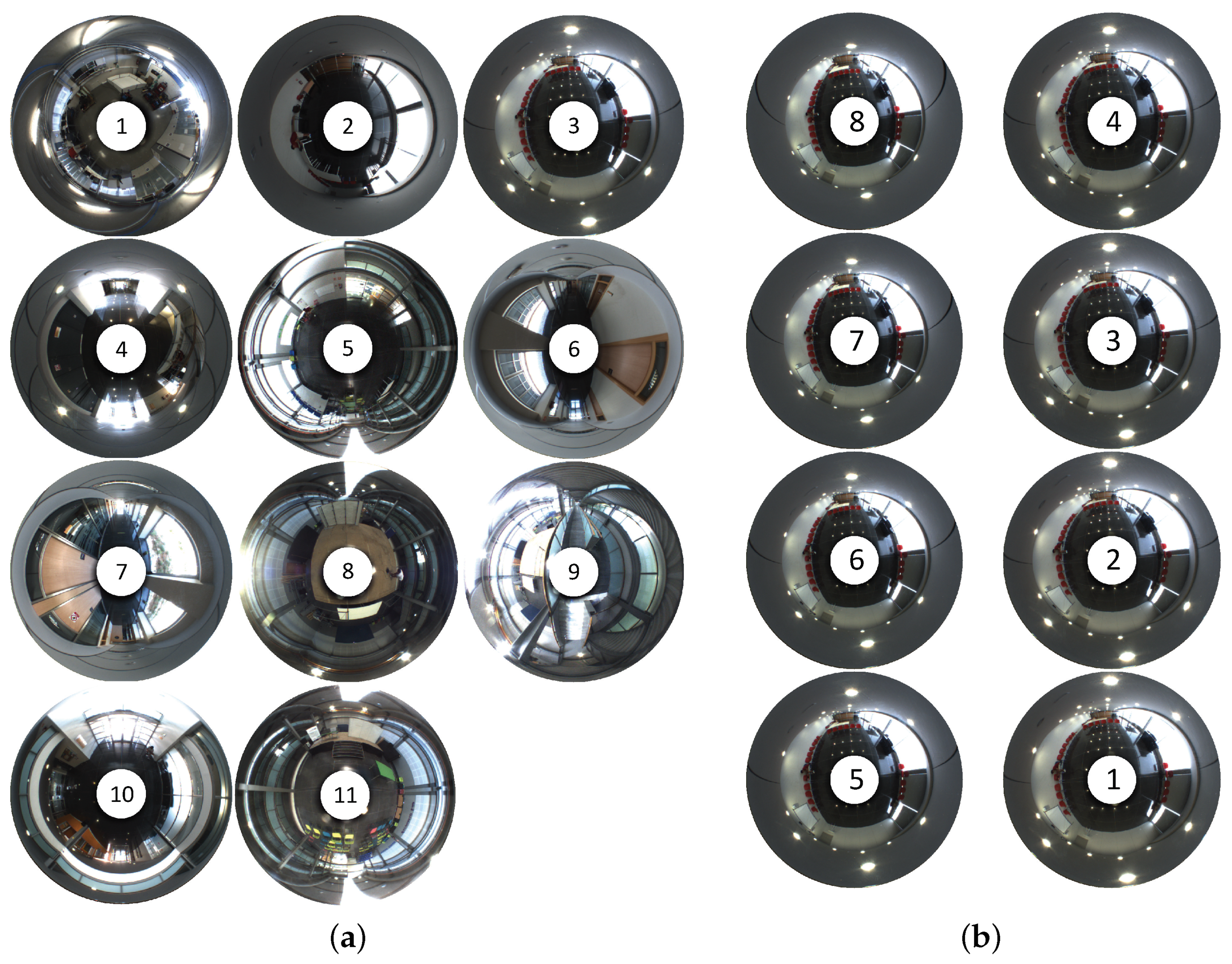
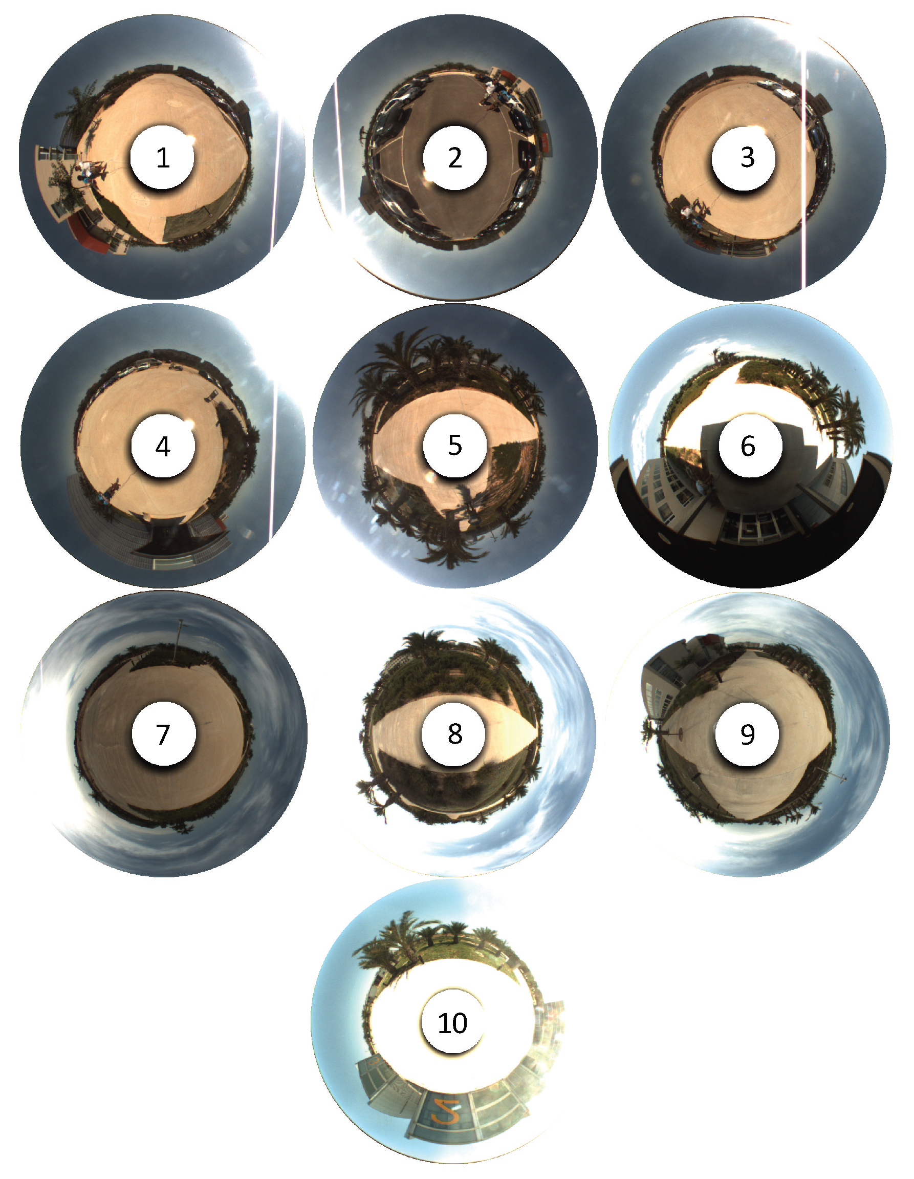
The indoor environments have been chosen to cover a variety of situations: both wide and narrow areas; structured and unstructured environments. Furthermore, the coordinates have been chosen to cover a variety of situations outdoors: both close to buildings and in open spaces. Some sample images can be seen in Figure 10 and Figure 11 The whole set of images is fully accessible and downloadable from [39].
6. Experiments and Results
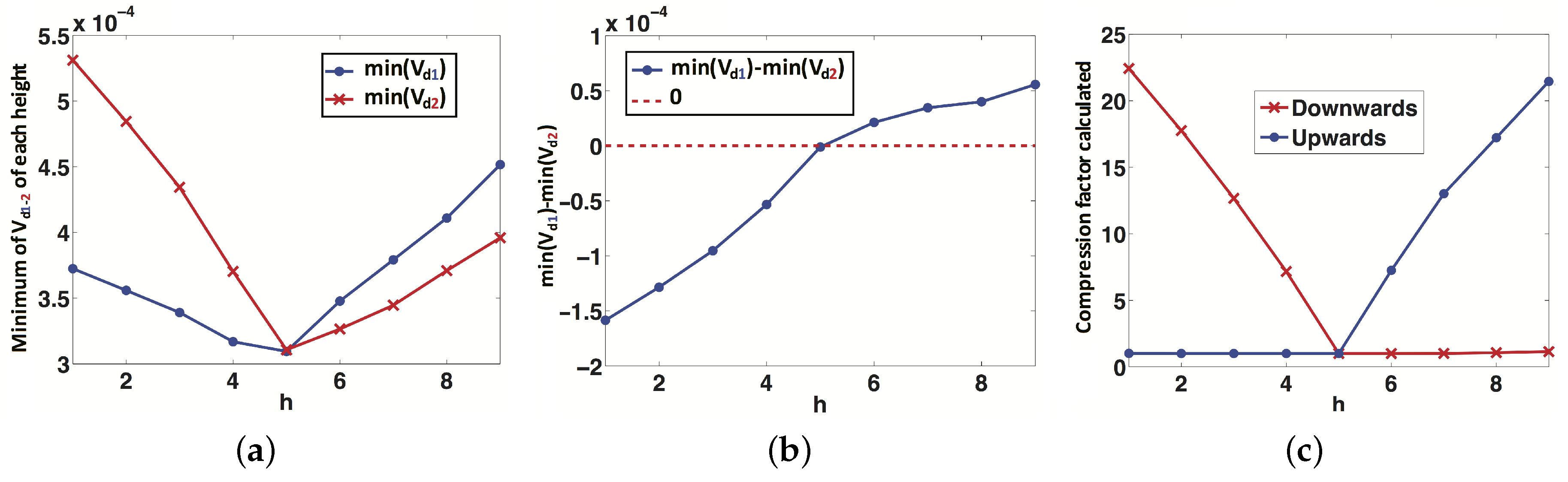
In this section, the results of the experiments with our altitude estimation method are shown. As presented in Section 4, an important step of the algorithm is to know the direction of the displacement (upwards or downwards). To make this distinction, the robot has to calculate the difference between two values: . This difference determines which is the absolute minimum, and it determines which is the correct direction.
Figure 12 shows an example of this process to obtain the direction of displacement, using the virtual environment. In this figure, the image captured at 1.85 m (h = 5) is the reference image, and all the other images are considered individually as test images and compared with the reference. Figure 12a shows, for each height h, the minimum of the vectors (Case 1, blue color) and (Case 2, red color). Figure 12b shows the difference between and . If this difference is positive, the correct case is Case 1 (upwards), and if it is negative, the correct case is Case 2 (downwards). In Figure 12c, the compression factor is represented versus the height h of the test image in both cases. This factor is an estimator of the topological height of the test image with respect to the reference image; therefore, it is proportional to the real relative height between both images. An example of this can be observed in Figure 12b, where the correct case for heights lower than 1.85 m (h = 5) is Case 1 (downwards) and for heights higher than 1.85 m is Case 2 (upwards), as expected. In Figure 12c, the red line to the left of h = 5 indicates the translation magnitude downwards from the reference image, and the blue line to the right of h = 5 indicates the translation magnitude upwards from the reference image. We can observe that the functions are quite linear.
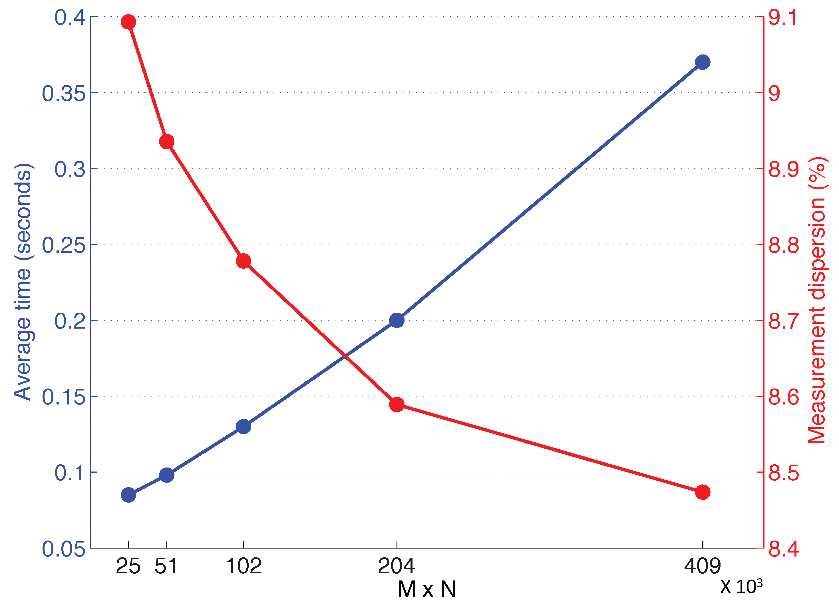
After this, an experiment has been developed to study the computational time of the height estimation algorithm and to optimize the size of the Radon transform descriptor. Figure 13 shows the results of this experiment. The blue curve represents the average time spent in each altitude estimation using the algorithm with different Radon transform sizes (), where M is the number of orientations considered to cover the whole circumference while calculating the Radon transform and N is the number of parallel lines considered at each orientation to calculate the integral along image intensities. In the horizontal axis of the figure, the next sizes are considered: . Furthermore, the red curve shows an uncertainty measurement calculated as the average between the standard deviation of the altitude estimated using eight different heights in each indoor environment. To do the subsequent experiments, we have chosen a Radon transform size of , because it presents a good balance between computational cost and uncertainty. In this case, the necessary time to complete the whole height estimation process is around s.
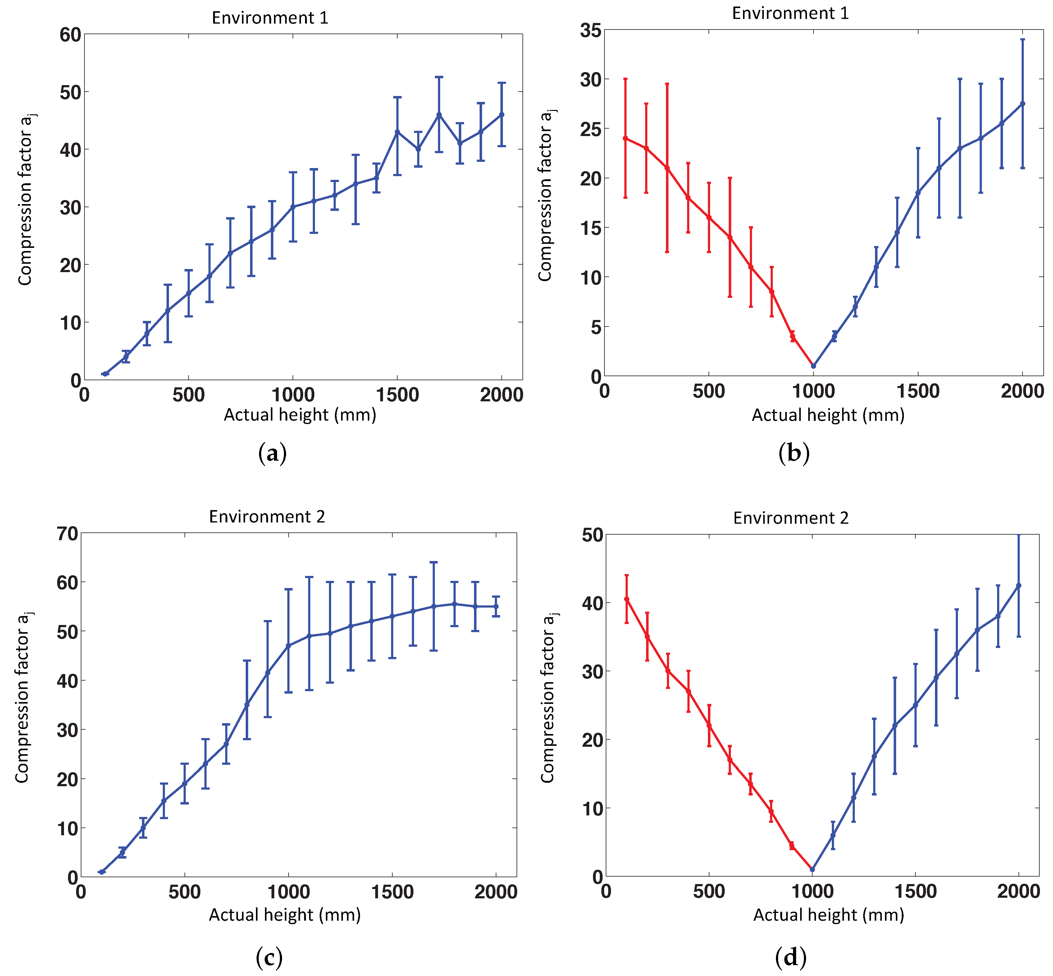
To test the validity and the correct performance of the method, we have done some experiments using omnidirectional images of both virtual environments. Fourteen positions have been selected randomly on the floor of these environments, and 20 images per position have been captured, changing only the altitude with respect to each position, with a height gap of 100 mm between consecutive images. In Figure 14, the global results of these experiments can be observed. The value of our topological height estimator is represented versus the actual metric height of the test image. The red line shows the relative translation when the direction is upwards, and the blue line shows the relative translation when the direction is downwards (in both cases, is a magnitude, which is proportional to the real translation). We can observe that these experiments prove that the method is very linear for values of relative height around or under 1 m. After the validation of the method using virtual environments, it is necessary to test it using the database composed of omnidirectional images taken in actual environments. To do this, we have used the database described in Section 5.2. We have considered also the possible presence of noise and occlusions in the test images, as they are a usual phenomena a mobile robot has to cope with when moving autonomously in a real working environment. We have considered random noise with maximum value equal to 20% of the maximum intensity of the omnidirectional image and occlusions that hide 15% of the omnidirectional image, at most.
Different reference images have been used to prove the correct performance estimating the altitude in both directions (upwards and downwards). One of the reference images has been taken at 1250 mm (h = 1) and the another one at 1850 mm (h = 5).
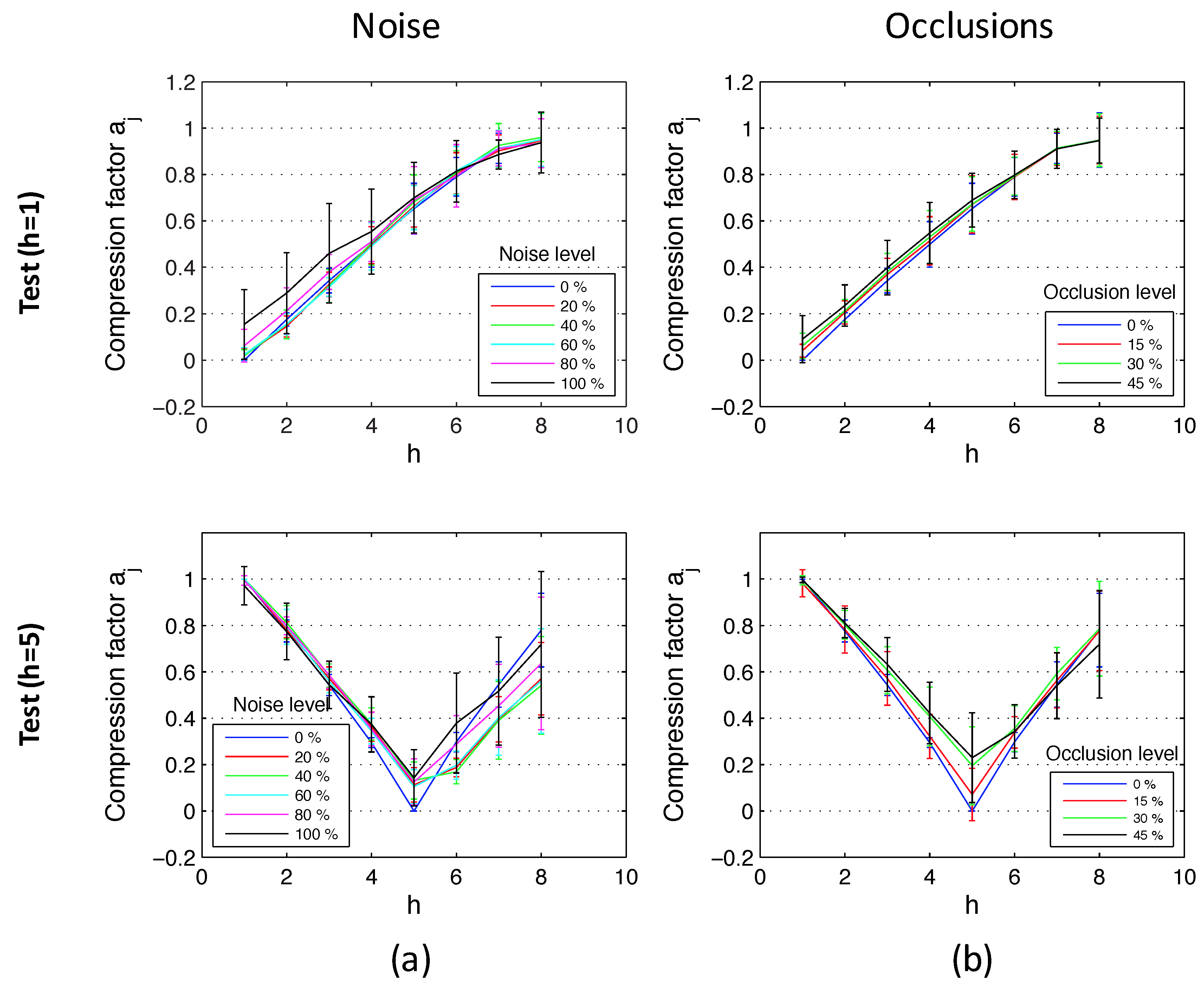
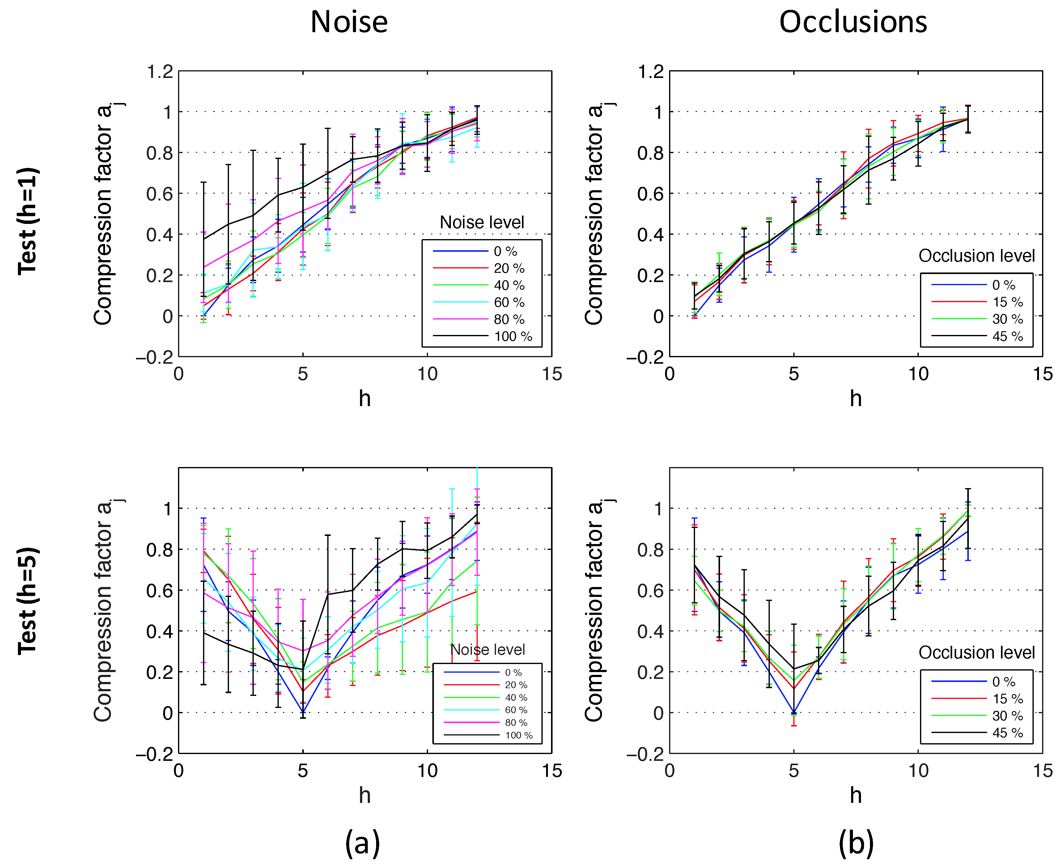
Figure 15 shows the results of the experiments using the database that contains indoor environments (Figure 10). This figure shows the average and the standard deviation of all location estimations by adding different levels of noise (random noise whose maximum value depends on the maximum value of the test image pixels intensity; Figure 15a) and with the presence of different occlusions (the occlusions cover a percentage of the test image; Figure 15b). The compression factors in each experiment have been normalized with respect to the maximum factor in each environment. At last, Figure 16 shows the same experiments using the database captured in outdoor environments (Figure 11). It contains more test points than the indoor database because there are no ceiling limitations in outdoor environments. This way, these figures permit testing the performance of the method for different magnitudes of movement. The horizontal axes show the value of h, which indicates the height where each test image is captured. As stated in Section 5, h = 1 corresponds to a height of 1250 mm, h = 2 corresponds to 1400 mm, etc. There is a gap of 150 mm between consecutive values of h. Figure 15 shows that the behavior of the method in indoor environments is robust. The height indicator proves to be relatively linear (even when severe noise or occlusions are present) and constant (the presence of these disturbing phenomena do not change substantially the behavior of the indicators). Regarding the behavior in outdoor environments, the indicator is robust against the presence of occlusions and moderate noise. However, the presence of severe noise changes the behavior of the indicator (which presents a lower slope under the presence of high levels of noise). Anyway, even in that case, the indicator presents a monotonously-increasing behavior with respect to the reference image.
The results show that the proposed method is able to estimate the topological altitude of the robot using only one omnidirectional vision sensor. Furthermore, it goes beyond the topological concept of connectivity; the method provides a height measure, which is proportional to the geometrical altitude of the robot (except for a scale factor). It is important to highlight the fact that, since the global appearance of the images is used and a topological approach is considered, the calibration of the camera and the stability of its parameters are not critical. Comparing to a previous work that used global appearance descriptors to estimate relative height [40], the present work presents some advantages. First, the orientation of the robot can be different for the reference and the test images, because POC is able to calculate and compensate this difference in orientation. In [40], the images have to be equally orientated to estimate correctly the relative height. Second, among the methods presented in [40], those based on the use of the orthographic view present the best performance, similar to the performance of the Radon transform. However, the computation time necessary to describe and compare the reference and the test images is substantially higher in [40] than in the present paper, where this time is around 0.2 s.
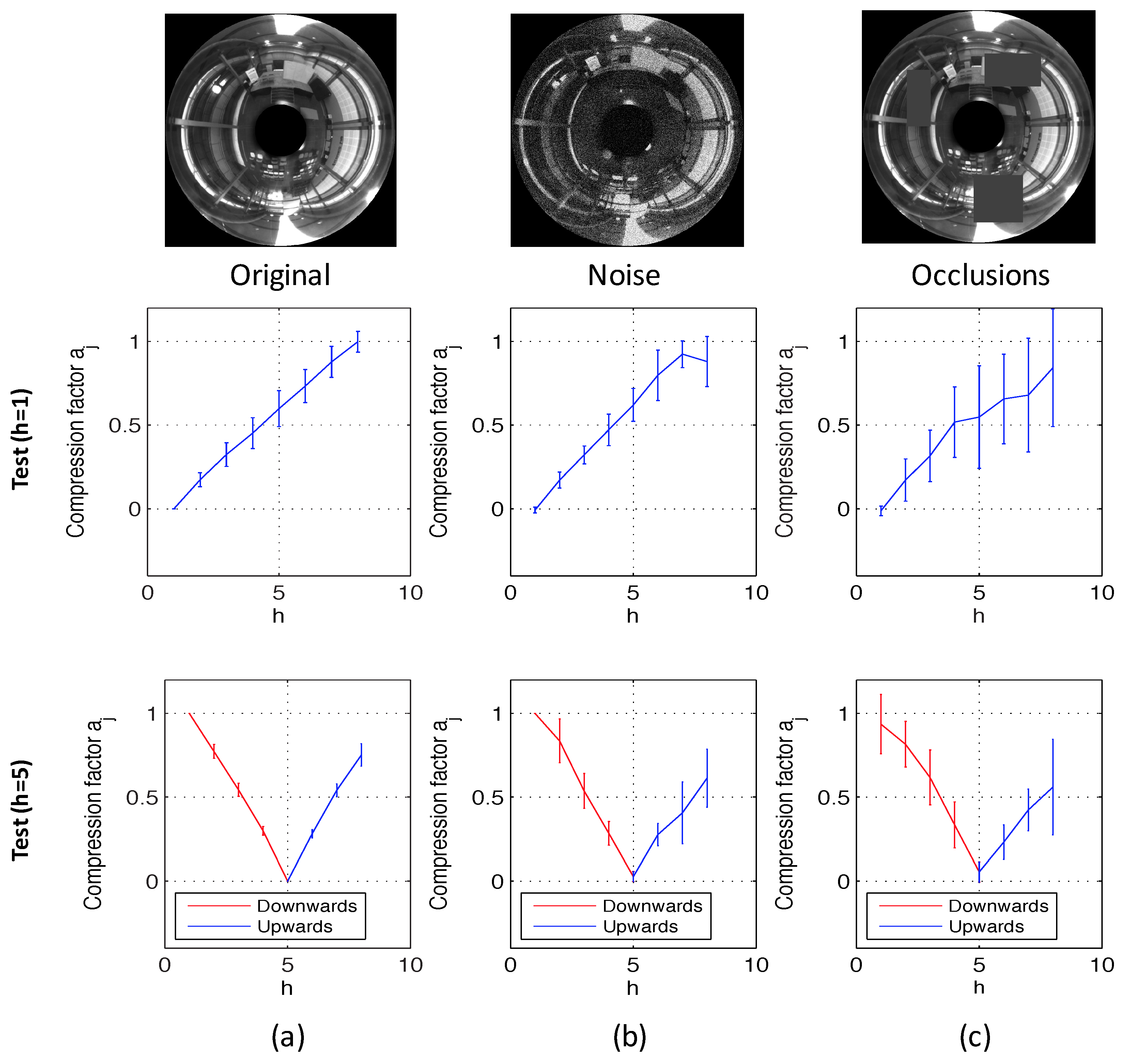
Finally, the method based on Radon transform has been compared with the benchmarking method described in Section 4.2. First of all, as far as the computational time is concerned, the method based on local features takes, on average, 1.3 s when SURF is used and 6.1 s when ASIFT is used. The global appearance method we propose takes 0.2 s on average, when the Radon transform has components (Figure 13). Second, the accuracy of the method in height estimation is studied. Figure 17 shows the same experiments as in Figure 15, but using the local features method and SURF. To obtain Figure 17, the maximum level of noise is of the maximum pixel intensity value of the test image, and the occlusions cover of the image. Comparing both frameworks, the method based on global appearance presents a more linear evolution when such moderate levels of noise and occlusions are present, and the deviation of the results tends to be lower. When the test image does not present noise nor occlusions, the result of both methods is quite similar, as far as linearity and deviation are concerned. Nevertheless, the global appearance method presents a substantially lower computational cost in all cases. Figure 18 shows the results of the same experiments as in Figure 17, but using the outdoor environments (Figure 11). In this case, when the reference image is at h = 5, the slope of the height estimator changes substantially for downwards and upwards movements.
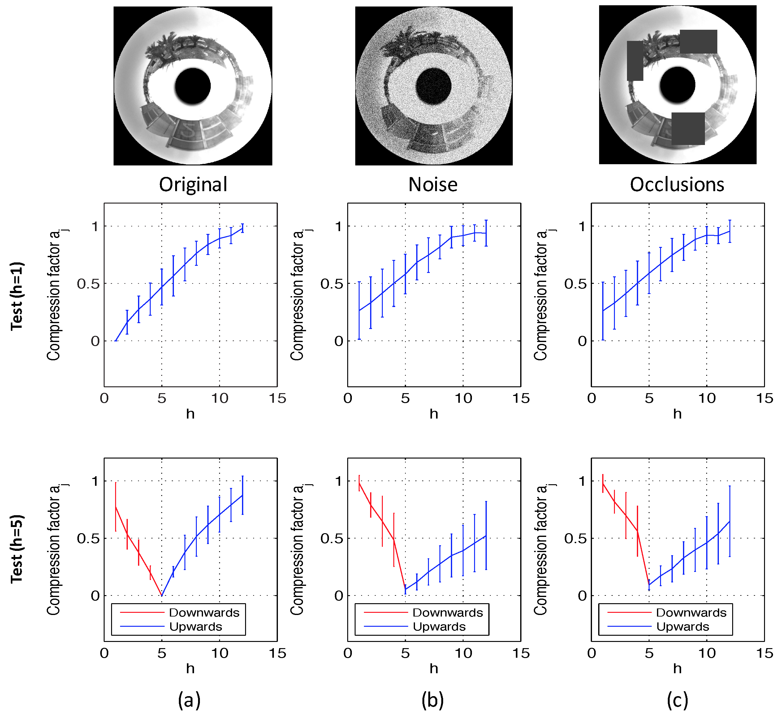
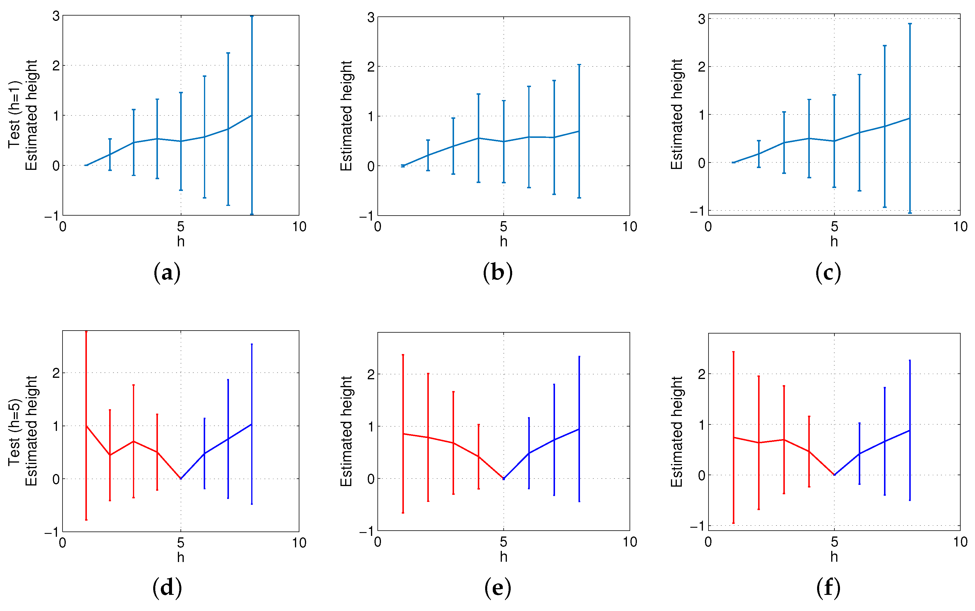
To conclude the experimental section, the method based on Radon transform is compared with the benchmarking method based on ASIFT features. As stated in the previous paragraph, the method based on ASIFT takes, on average, 6.1 s to compare both images and provide the height estimation, while the method based on Radon transform takes 0.2 s. Figure 19 shows the results of the ASIFT benchmarking method when the indoors dataset is considered and Figure 20 with the outdoors dataset. In both figures, the maximum level of noise considered is of the maximum pixel intensity value of the test image, and the occlusions cover of the image. In this case, the benchmarking method presents relatively linear results in indoor environments, even in the presence of noise or occlusions. However, the ASIFT method loses linearity and presents a substantially higher standard deviation when the outdoors database is used, even when the original test images are used (with neither noise nor occlusions added to the test images). Figure 20d shows clearly this effect when the robot moves downwards (red curve).
7. Conclusions
In this work, a method to estimate the relative altitude of a mobile robot has been presented. The Radon transform of omnidirectional images is used by this method to build a global appearance descriptor per image. Furthermore, the method compares the descriptors and finally estimates the relative height of the robot, considering the changes that Radon transforms of images experience when the robot changes its height. A remarkable aspect is that the method is able to detect these height changes both in indoor and outdoor environments using the same map as is used in localization tasks. Furthermore, this approach permits estimating the height of the robot even when it is has a rotation with respect to the floor plane because the POC comparison permits estimating and correcting this rotation.
The experiments developed in this paper use our own sets of images created from two different virtual environments. Furthermore, experiments using actual databases have been carried out to test the validity of the method in indoor and outdoor actual environments, even using images with noise and occlusions. The results demonstrate that the method is able to estimate the relative altitude between two omnidirectional images with robustness and linearity even in the presence of noise and occlusions. Furthermore, the method is able to estimate the relative altitude of the robot in a reasonable amount of time. It would permit navigation in real time.
The method has been compared with an alternative method based on the classical framework of extracting, comparing, and tracking local features. The results have shown that the global appearance method we propose outperforms the local features method and presents a lower computational cost.
The results of this work encourage us to continue this research line. Once the method based on the Radon transform has proven to be a feasible alternative, we are working on the design of a complete visual odometry framework using this descriptor. Additionally, the team is planning to extend the algorithm to estimate movements with six degrees of freedom. It would lead to the creation of a complete SLAM algorithm using this kind of descriptor.
Author Contributions
Conceptualization, L.P. and O.R.; methodology, Y.B., L.P., and O.R.; software, Y.B., D.V., and A.P.; validation, Y.B., D.V., and A.P.; formal analysis, L.P. and O.R.; investigation, Y.B., L.P., and O.R.; resources, O.R. and L.P.; data curation, Y.B., A.P., and D.V.; writing, original draft preparation, Y.B. and L.P.; writing, review and editing, O.R., A.P., and D.V.; visualization, Y.B., D.V., and A.P.; supervision, L.P. and O.R.; project administration, L.P. and O.R.; funding acquisition, L.P. and O.R.
Funding
This research was funded by the Spanish Government through the project DPI2016-78361-R (AEI/FEDER, UE): “Creación de Mapas Mediante Métodos de Apariencia Visual para la Navegación de Robots.
Conflicts of Interest
The authors declare no conflict of interest. The funders had no role in the design of the study; in the collection, analyses, or interpretation of data; in the writing of the manuscript; nor in the decision to publish the results.
Abbreviations
The following abbreviations are used in this manuscript:
| GPS | Global Positioning System |
| IMU | Inertial Measurement Unit |
| SIFT | Scale-Invariant Feature Transform |
| SURF | Speeded-Up Robust Features |
| ASIFT | Affine Scale-Invariant Feature Transform |
| SLAM | Simultaneous Localization and Mapping |
| UAV | Unmanned Aerial Vehicle |
| POC | Phase-Only Correlation |
| RANSAC | Random Sample Consensus |
References
- Garcia-Fidalgo, E.; Ortiz, A. Vision-based topological mapping and localization methods: A survey. Robot. Auton. Syst. 2015, 64, 1–20. [Google Scholar] [CrossRef]
- Winters, N.; Gaspar, J.; Lacey, G.; Santos-Victor, J. Omni-directional vision for robot navigation. In Proceedings of the IEEE Workshop on Omnidirectional Vision, Hilton Head Island, SC, USA, 12 June 2000; pp. 21–28. [Google Scholar]
- Oriolo, G.; Paolillo, A.; Rosa, L.; Vendittelli, M. Humanoid odometric localization integrating kinematic, inertial and visual information. Auton. Robot. 2016, 40, 867–879. [Google Scholar] [CrossRef]
- Satici, A.; Tick, D.; Shen, J.; Gans, N. Path-following control for mobile robots localized via sensor-fused visual homography. In Proceedings of the 2013 American Control Conference, Washington, DC, USA, 17–19 June 2013; pp. 6287–6293. [Google Scholar]
- Caruso, D.; Engel, J.; Cremers, D. Large-scale direct slam for omnidirectional cameras. In Proceedings of the 2015 IEEE/RSJ International Conference on Intelligent Robots and Systems (IROS), Hamburg, Germany, 28 September–2 October 2015; pp. 141–148. [Google Scholar]
- Corke, P.; Strelow, D.; Singh, S. Omnidirectional visual odometry for a planetary rover. In Proceedings of the IEEE/RSJ International Conference on Intelligent Robots and Systems, 2004 (IROS 2004), Sendai, Japan, 28 September–2 October 2004; Volume 4, pp. 4007–4012. [Google Scholar]
- Lowe, D. Object Recognition from local scale-invariant features. In Proceedings of the Seventh IEEE International Conference on Computer Vision, Kerkyra, Greece, 20–27 September 1999; Volume 2, pp. 1150–1157. [Google Scholar]
- Bay, H.; Tuytelaars, T.; Gool, L. SURF: Speeded up robust features. In Proceedings of the Computer Vision at ECCV 2006, Graz, Austria, 7–13 May 2006; Volume 3951, pp. 404–417. [Google Scholar]
- Hansen, P.; Corket, P.; Boles, W.; Daniilidis, K. Scale invariant feature matching with wide angle images. In Proceedings of the IEEE/RSJ International Conference on Intelligent Robots and Systems, San Diego, CA, USA, 10 December 2007; pp. 1689–1694. [Google Scholar]
- Morel, J.M.; Yu, G. ASIFT: A new framework for fully affine invariant image comparison. SIAM J. Imaging Sci. 2009, 2, 438–469. [Google Scholar] [CrossRef]
- Puig, L.; Guerrero, J.J. Scale space for central catadioptric systems: Towards a generic camera feature extractor. In Proceedings of the 2011 IEEE International Conference on Computer Vision (ICCV), Barcelona, Spain, 12 January 2012; pp. 1599–1606. [Google Scholar]
- Jiang, Y.; Xu, Y.; Liu, Y. Performance evaluation of feature detection and matching in stereo visual odometry. Neurocomputing 2013, 120, 380–390. [Google Scholar] [CrossRef]
- Payá, L.; Fernández, L.; Gil, L.; Reinoso, O. Map building and Monte Carlo localization using global appearance of omnidirectional images. Sensors 2010, 10, 11468–11497. [Google Scholar] [CrossRef]
- Payá, L.; Reinoso, O.; Berenguer, Y.; Úbeda, D. Using Omnidirectional Vision to Create a Model of the Environment: A Comparative Evaluation of Global-Appearance Descriptors. J. Sens. 2016, 2016, 1209507. [Google Scholar] [CrossRef]
- Fernández, L.; Payá, L.; Reinoso, O.; Jimenez, L.M. Appearance-based approach to hybrid metric-topological simultaneous localisation and mapping. IET Intell. Transp. Syst. 2014, 8, 688–699. [Google Scholar] [CrossRef]
- Munguía, R.; Urzua, S.; Bolea, Y.; Grau, A. Vision-Based SLAM System for Unmanned Aerial Vehicles. Sensors 2016, 16, 372. [Google Scholar] [CrossRef]
- Forster, C.; Lynen, S.; Kneip, L.; Scaramuzza, D. Collaborative monocular SLAM with multiple Micro Aerial Vehicles. In Proceedings of the 2013 IEEE/RSJ International Conference on Intelligent Robots and Systems, Tokyo, Japan, 3–7 November 2013; pp. 3962–3970. [Google Scholar] [CrossRef]
- Weiss, S.; Achtelik, M.W.; Chli, M.; Siegwart, R. Versatile distributed pose estimation and sensor self-calibration for an autonomous MAV. In Proceedings of the 2012 IEEE International Conference on Robotics and Automation (ICRA), Saint Paul, MN, USA, 14–18 May 2012; pp. 31–38. [Google Scholar] [CrossRef]
- Bunschoten, R.; Krose, B. Robust scene reconstruction from an omnidirectional vision system. IEEE Trans. Robot. Autom. 2003, 19, 351–357. [Google Scholar] [CrossRef]
- Drews, P., Jr.; Botelho, S.; Gomes, S. SLAM in Underwater Environment Using SIFT and Topologic Maps. In Proceedings of the 2008 IEEE Latin American Robotic Symposium, Natal, Brazil, 29–30 October 2008; pp. 91–96. [Google Scholar] [CrossRef]
- Kostavelis, I.; Charalampous, K.; Gasteratos, A.; Tsotsos, J.K. Robot navigation via spatial and temporal coherent semantic maps. Eng. Appl. Artif. Intell. 2016, 48, 173–187. [Google Scholar] [CrossRef]
- Dayoub, F.; Morris, T.; Upcroft, B.; Corke, P. Vision-only autonomous navigation using topometric maps. In Proceedings of the 2013 IEEE/RSJ International Conference on Intelligent Robots and Systems (IROS), Tokyo, Japan, 3–7 November 2013; pp. 1923–1929. [Google Scholar] [CrossRef]
- Berenguer, Y.; Payá, L.; Ballesta, M.; Reinoso, O. Position Estimation and Local Mapping Using Omnidirectional Images and Global Appearance Descriptors. Sensors 2015, 15, 26368–26395. [Google Scholar] [CrossRef] [PubMed]
- Kuglin, C.; Hines, D. The phase correlation image alignment method. In Proceedings of the IEEE International Conference on Cybernetics and Society, San Francisco, CA, USA, 23–25 September 1975; pp. 163–165. [Google Scholar]
- Kim, J.H.; Kwon, J.W.; Seo, J. Multi-UAV-based stereo vision system without GPS for ground obstacle mapping to assist path planning of UGV. Electron. Lett. 2014, 50, 1431–1432. [Google Scholar] [CrossRef]
- Angelino, C.V.; Baraniello, V.R.; Cicala, L. High altitude UAV navigation using IMU, GPS and camera. In Proceedings of the 2013 16th International Conference on Information Fusion (FUSION), Istanbul, Turkey, 9–12 July 2013; pp. 647–654. [Google Scholar]
- Amorós, F.; Payá, L.; Reinoso, O.; Valiente, D. Towards relative altitude estimation in topological navigation tasks using the global appearance of visual information. In Proceedings of the VISAPP 2014 International Conference on Computer Vision Theory and Applications, Lisbon, Portugal, 5–8 January 2014; Volume 1, pp. 194–201. [Google Scholar]
- Ranganathan, A.; Menegatti, E.; Dellaert, F. Bayesian inference in the space of topological maps. IEEE Trans. Robot. 2006, 22, 92–107. [Google Scholar] [CrossRef]
- Menegatti, E.; Zoccarato, M.; Pagello, E.; Ishiguro, H. Image-based Monte Carlo localisation with omnidirectional images. Robot. Auton. Syst. 2004, 48, 17–30. [Google Scholar] [CrossRef]
- Mondragon, I.; Olivares-Ménded, M.; Campoy, P.; Martínez, C.; Mejias, L. Unmanned aerial vehicles UAVs attitude, height, motion estimation and control using visual systems. Auton. Robot. 2010, 29, 17–34. [Google Scholar] [CrossRef]
- Natraj, A.; Ly, D.S.; Eynard, D.; Demonceaux, C.; Vasseur, P. Omnidirectional Vision for UAV: Applications to Attitude, Motion and Altitude Estimation for Day and Night Conditions. J. Intell. Robot. Syst. 2012, 69, 459–473. [Google Scholar] [CrossRef]
- Payá, L.; Amorós, F.; Fernández, L.; Reinoso, O. Performance of Global-Appearance Descriptors in Map Building and Localization Using Omnidirectional Vision. Sensors 2014, 14, 3033–3064. [Google Scholar] [CrossRef] [PubMed]
- Radon, J. Uber die bestimmung von funktionen durch ihre integralwerte langs gewisser mannigfaltigkeiten. Ber. Sachs. Akad. Wiss. 1917, 69, 262–277. [Google Scholar]
- Berenguer, Y.; Payá, L.; Peidro, A.; Reinoso, O. Relative height estimation using omnidirectional images and a global appearance approach. In Proceedings of the 2015 12th International Conference on Informatics in Control, Automation and Robotics (ICINCO), Colmar, France, 21–23 July 2015; Volume 2, pp. 202–209. [Google Scholar]
- Hoang, T.; Tabbone, S. A Geometric Invariant Shape Descriptor Based on the Radon, Fourier, and Mellin Transforms. In Proceedings of the 2010 20th International Conference on Pattern Recognition (ICPR), Istanbul, Turkey, 23–26 August 2010; pp. 2085–2088. [Google Scholar] [CrossRef]
- Hasegawa, M.; Tabbone, S. A Shape Descriptor Combining Logarithmic-Scale Histogram of Radon Transform and Phase-Only Correlation Function. In Proceedings of the 2011 International Conference on Document Analysis and Recognition (ICDAR), Beijing, China, 18–21 September 2011; pp. 182–186. [Google Scholar] [CrossRef]
- Menegatti, E.; Maeda, T.; Ishiguro, H. Image-based memory for robot navigation using properties of omnidirectional images. Robot. Auton. Syst. 2004, 47, 251–267. [Google Scholar] [CrossRef]
- Oppenheim, A.; Lim, J. The importance of phase in signals. Proc. IEEE 1981, 69, 529–541. [Google Scholar] [CrossRef]
- Payá, L.; Amorós, F.; Fernández, L.; Reinoso, O. Miguel Hernandez University. Set of Images for Altitude Estimation. 2014. Available online: http://arvc.umh.es/db/images/altitude/ (accessed on 26 December 2018).
- Amorós, F.; Payá, L.; Ballesta, M.; Reinoso, O. Development of Height Indicators using Omnidirectional Images and Global Appearance Descriptors. Appl. Sci. 2017, 7, 482. [Google Scholar] [CrossRef]
Figure 1.
Line parametrization through the distance to the origin d and the angle between the normal line and the x axis, .
Figure 1.
Line parametrization through the distance to the origin d and the angle between the normal line and the x axis, .

Figure 2.
World and robot reference systems. A change in the height is shown (the robot moves from to ).
Figure 2.
World and robot reference systems. A change in the height is shown (the robot moves from to ).

Figure 3.
Example of the Radon transform compression effect. The figure shows the omnidirectional image and its Radon transform captured at (a) h = 1.25 m and (b) h = 2 m. Comparing both Radon transforms, the second one presents a compression effect with respect to the first one.
Figure 3.
Example of the Radon transform compression effect. The figure shows the omnidirectional image and its Radon transform captured at (a) h = 1.25 m and (b) h = 2 m. Comparing both Radon transforms, the second one presents a compression effect with respect to the first one.

Figure 4.
(a) Omnidirectional image captured from a specific position of the environment and its Radon transform. (b) Omnidirectional image taken from the same location changing only the robot orientation around the axis and its Radon transform. A change of the robot orientation around the axis produces a shift of the columns of the Radon transform, .

Figure 5.
Flowchart of the altitude estimation method.

Figure 6.
Matches between the reference image (left) and the test image (right) in an indoor environment. The red circles are the valid landmarks in the reference image, and the green crosses are the valid landmarks in the test image.
Figure 6.
Matches between the reference image (left) and the test image (right) in an indoor environment. The red circles are the valid landmarks in the reference image, and the green crosses are the valid landmarks in the test image.

Figure 7.
Angular differences between the direction between each landmark in the reference image and the center of the image and the direction between the matched landmark in the test image and the center of the image.
Figure 7.
Angular differences between the direction between each landmark in the reference image and the center of the image and the direction between the matched landmark in the test image and the center of the image.

Figure 8.
Final step of the alternative method. The red-colored image is the reference image, and the blue colored is the test image. The red circles are the final landmarks in the reference image (after removing outliers), and the green crosses are the valid landmarks in the test image.
Figure 8.
Final step of the alternative method. The red-colored image is the reference image, and the blue colored is the test image. The red circles are the final landmarks in the reference image (after removing outliers), and the green crosses are the valid landmarks in the test image.

Figure 9.
(a) Omnidirectional acquisition system. (b) Model of the virtual hyperbolic mirror used to capture the synthetic omnidirectional images.
Figure 9.
(a) Omnidirectional acquisition system. (b) Model of the virtual hyperbolic mirror used to capture the synthetic omnidirectional images.

Figure 10.
(a) One sample omnidirectional image per indoor environment is shown. (b) Images captured in Indoor Environment 3 from the maximum altitude (eight) to the minimum altitude (one).
Figure 10.
(a) One sample omnidirectional image per indoor environment is shown. (b) Images captured in Indoor Environment 3 from the maximum altitude (eight) to the minimum altitude (one).

Figure 11.
One sample omnidirectional image per outdoor environments is shown.

Figure 12.
(a) Minimum of the vectors (Case 1) and (Case 2). (b) Difference between and . (c) The factor, which is proportional to the real relative height between each image and the test image. This example has been carried out using an indoor environment of the virtual dataset.
Figure 12.
(a) Minimum of the vectors (Case 1) and (Case 2). (b) Difference between and . (c) The factor, which is proportional to the real relative height between each image and the test image. This example has been carried out using an indoor environment of the virtual dataset.

Figure 13.
Average time and measurement dispersion using different Radon transform sizes. All indoor environments have been used to carry out these comparisons by calculating eight different altitude estimations in each environment.
Figure 13.
Average time and measurement dispersion using different Radon transform sizes. All indoor environments have been used to carry out these comparisons by calculating eight different altitude estimations in each environment.

Figure 14.
(a) Experiments in Virtual Environment 1 with the reference image at height = 100 mm. (b) Experiments in the environment 1 with the reference image at 1000 mm. (c) Experiments in the virtual environment 2 with the reference image at 100 mm. (d) Experiments in Environment 2 with the reference image at 1000 mm.

Figure 15.
Altitude estimation using the database captured in indoor environments, using reference images at the bottom (h = 1) and in the middle of the height (h = 5). Average and standard deviation of all locations considering (a) the original test images, (b) noise added to the test images, and noise + occlusions added to the test images.

Figure 16.
Altitude estimation using the database captured in outdoor environments, using reference images at the bottom (h = 1) and in the middle of the height (h = 5). Average and standard deviation of all locations considering (a) noise added to the test images and (b) occlusions added to the test images.

Figure 17.
Altitude estimation using the method based on SURF features and the indoors database, using reference images at the bottom (h = 1) and in the middle of the height (h = 5). Average and standard deviation of all locations considering (a) the original test images, (b) noise added to the test images and (c) occlusions added to the test images.

Figure 18.
Altitude estimation using the method based on SURF features and the outdoors database, using reference images at the bottom (h = 1) and in the middle of the height (h = 5). Average and standard deviation of all locations considering (a) the original test images, (b) noise added to the test images, and (c) occlusions added to the test images.

Figure 19.
Altitude estimation using the method based on ASIFT and the indoors dataset. Reference images at the bottom (h = 1) and (a) original test images, (b) noise added to the test images, and (c) occlusions added to the test images. Reference in the middle of the height (h = 5) and (d) original test images, (e) noise added to the test images, and (f) occlusions added to the test images.

Figure 20.
Altitude estimation using the method based on ASIFT and the outdoors dataset. Reference images at the bottom (h = 1) and (a) original test images, (b) noise added to the test images, and (c) occlusions added to the test images. Reference in the middle of the height (h = 5) and (d) original test images, (e) noise added to the test images, and (f) occlusions added to the test images.

© 2019 by the authors. Licensee MDPI, Basel, Switzerland. This article is an open access article distributed under the terms and conditions of the Creative Commons Attribution (CC BY) license (http://creativecommons.org/licenses/by/4.0/).
Share and Cite
MDPI and ACS Style
Berenguer, Y.; Payá, L.; Valiente, D.; Peidró, A.; Reinoso, O. Relative Altitude Estimation Using Omnidirectional Imaging and Holistic Descriptors. Remote Sens. 2019, 11, 323. https://0-doi-org.brum.beds.ac.uk/10.3390/rs11030323
AMA Style
Berenguer Y, Payá L, Valiente D, Peidró A, Reinoso O. Relative Altitude Estimation Using Omnidirectional Imaging and Holistic Descriptors. Remote Sensing. 2019; 11(3):323. https://0-doi-org.brum.beds.ac.uk/10.3390/rs11030323
Chicago/Turabian StyleBerenguer, Yerai, Luis Payá, David Valiente, Adrián Peidró, and Oscar Reinoso. 2019. "Relative Altitude Estimation Using Omnidirectional Imaging and Holistic Descriptors" Remote Sensing 11, no. 3: 323. https://0-doi-org.brum.beds.ac.uk/10.3390/rs11030323
Note that from the first issue of 2016, this journal uses article numbers instead of page numbers. See further details here.