Improving the Performance of Galileo Uncombined Precise Point Positioning Ambiguity Resolution Using Triple-Frequency Observations

Abstract

Compared with the traditional ionospheric-free linear combination precise point positioning (PPP) model, the un-differenced and uncombined (UDUC) PPP model using original observations can keep all the information of the observations and be easily extended to any number of frequencies. However, the current studies about the multi-frequency UDUC-PPP ambiguity resolution (AR) were mainly based on the triple-frequency BeiDou navigation satellite system (BDS) observations or simulated data. Limited by many factors, for example the accuracy of BDS precise orbit and clock products, the advantages of triple-frequency signals to UDUC-PPP AR were not fully exploited. As Galileo constellations have been upgraded by increasing the number of 19 useable satellites, it makes using Galileo satellites to further study the triple-frequency UDUC-PPP ambiguity resolution (AR) possible. In this contribution, we proposed the method of multi-frequency step-by-step ambiguity resolution based on the UDUC-PPP model and gave the reason why the performance of PPP AR can be improved using triple-frequency observations. We used triple-frequency Galileo observations on day of year (DOY) 201, 2018 provided by 166 Multi-GNSS Experiment (MGEX) stations to estimate original uncalibrated phase delays (UPD) on each frequency and to conduct both dual- and triple-frequency UDUC-PPP AR. The performance of UDUC-PPP AR based on post-processing mode was assessed in terms of the time-to-first-fix (TTFF) as well as positioning accuracy with 2-h observations. It was found that triple-frequency observations were helpful to reduce TTFF and improve the positioning accuracy. The current statistic results showed that triple-frequency PPP-AR reduced the averaged TTFF by 19.6% and also improved the positioning accuracy by 40.9%, 31.2% and 23.6% in the east, north and up directions respectively, compared with dual-frequency PPP-AR. With an increasing number of Galileo satellites, it is expected that the robustness and accuracy of the triple-frequency UCUD-PPP AR can be improved further.

1. Introduction

The precise point positioning (PPP) technique has drawn a lot of attention from the Global Navigation Satellite Systems (GNSS) community due to its flexible operation, permitting centimeter- to millimeter-level positioning accuracy with a single receiver and unlimited coverage, which has been widely used for engineering applications and scientific research for many years [1]. Taking advantage of the integer property of the GNSS carrier phase ambiguity through proper handling of satellite and receiver phase delays, the PPP ambiguity resolution (AR) could further reduce convergence time and improve positioning accuracy [2,3,4]. However, current dual-frequency PPP AR still needs a comparatively long initialization and cannot reach the same instantaneous ambiguity resolution and accuracy as the Network-based real-time kinematic (NRTK) positioning technique [5]. With new generations of global navigation satellite system (GNSS) space vehicles transmitting three or more frequency signals, the extra frequency signals are expected to bring significant improvement to the time-to-first-fix (TTFF) and positioning accuracy of PPP AR.

Early researches toward carrier phase AR using three or more signals mainly focused on theory and algorithms of precise relative positioning. Forssell et al. [6] and Vollath et al. [7] made the earliest studies and described the three-carrier ambiguity resolution (TCAR) method. De Jonge et al. [8] and Hatch et al. [9] proposed the cascaded integer resolution (CIR) method. The basic idea of the TCAR/CIR method is that AR starts with the easy-to-fix extra-wide-lane (EWL) combination and steps to the shorter wavelength wide-lane (WL) and narrow-lane (NL) combinations sequentially, in which the WL combination is used to bridge the longest wavelength EWL and the shortest wavelength NL [10]. This method was also further extended and modified by lots of follow-up studies e.g., References [11] or [12], [13] or [14] and [15]. Geng and Bock [16] put forward a triple-frequency AR method based on the idea of TCAR/CIR for an ionospheric-free (IF) linear combination PPP model. The PPP ambiguity resolution is also conducted by three steps, first EWL, then WL and finally NL ambiguity resolution. Their simulated results suggested that the correctness rate of NL AR achieved 99% within 65 s, compared with only 64% within 150 s in the traditional dual-frequency PPP-AR.

In recent years, the studies of multi-frequency PPP are changing from the traditional ionosphere-free combination model to the un-differenced and uncombined (UDUC) model which has the advantage of lower noise and also keeps all the information of the observations [17,18]. The UDUC-PPP model is also considered as the unified multi-GNSS and multi-frequency positioning model [17,19]. Gu et al. [20] studied the triple-frequency PPP-AR based on raw BDS observations. In their study, the satellite phase bias of EWL, WL and L1 ambiguities were first estimated based on the UDUC-PPP model and then the EWL and WL ambiguities with recovered integer property were fixed with LAMBDA method; however, the reliable fixing of the BDS L1 ambiguity faced difficulties. Li et al. [21] proposed a unified BeiDou navigation satellite system (BDS) uncalibrated phase delays (UPD) estimation and UDUC-PPP AR method. However, the results were limited by low precise orbits and clock products as well as the lack of precise BDS PCO+PCV corrections for both receivers and satellites. In addition, their research was only focused on the Asia-Pacific regions instead of the global scale. The above reviews reveal that the current studies about the contributions of triple-frequency signals to UDUC-PPP AR are still limited. As the number of Galileo constellation has increased to a total of 19 useable satellites, it gives us the great opportunity to further research on the improvement of UDUC-PPP AR using triple-frequency signals.

This paper aims to further research on the benefits of extra signals to improve the performance of the UDUC-PPP AR, using Galileo triple-frequency observations. To achieve this goal, we start with proposing the method of multi-frequency step-by-step ambiguity resolution which is based on the UDUC-PPP model. Subsequently, we show and analyze the results in terms of data acquisition, the characteristics of UPD estimates and the performance evaluation of dual- and triple-frequency UDUC-PPP AR. Finally, we summarize the main points and conclusions.

2. Methods

In this section, the UDUC-PPP AR method for clients will be briefly proposed. With triple-frequency measurements, the step-by-step AR can be divided into three cascaded steps, that is first EWL, then WL and finally NL AR. With dual-frequency measurements, AR is divided into two cascaded steps, which are first WL and then NL AR. The reason why we do not select the unified UDUC-PPP AR method which is based on the least-squares ambiguity decorrelation adjustment (LAMBDA) algorithm is that the Z-transformation leads to different linear ambiguity combinations forming according to the specific conditions for dual- and triple-frequency AR [21,22]. For example, linear ambiguity combinations generated by the Z-transformation for dual-frequency case are usually (1, 1) and (−7, 8), while linear ambiguity combinations for triple-frequency case are (0, 1, −1), (−2, 3, −1) and (−146, 162, −15) [23,24]. The different linear ambiguity combinations have the disadvantage of comparing the performance of dual- and triple-frequency AR. Therefore, the predefined combinations of the EWL-WL-NL and WL-NL strategies for dual- and triple-frequency UDUC-PPP AR respectively are beneficial to control the influence of different linear ambiguity combinations on the positioning results.

2.1. UDUC-PPP Observation Equation

The Galileo original pseudo-range and carrier-phase observation equation on frequency band g (g = 1, 2, 3) from station i (i = 1, … r) to satellite j (j = 1, … s) can be expressed as [16,25]

$$\{\begin{array}{l}{P}_{i,g}^j={\rho }_i^j+{\gamma }_g\cdot I_{i,1}^j+d_{i,g}-d^{j,g}+{\epsilon }_{i,g}^j\\ L_{i,g}^j={\rho }_i^j-{\gamma }_g\cdot I_{i,1}^j+{\lambda }_g\cdot (N_{i,g}^j+b_{i,g}-b^{j,g})+{\xi }_{i,g}^j\end{array}$$

(1)

where $P_{i,g}^j$ and $L_{i,g}^j$ denote the original pseudo-range and carrier-phase measurements in meters, respectively and ${\rho }_i^j$ denotes the non-dispersive delay including the geometric distance (m), the clock errors (m), the tropospheric delay (m), etc.; the antenna phase center corrections should be applied to $P_{i,g}^j$ and $L_{i,g}^j$ before ${\rho }_i^j$ becomes unassociated with the frequency. ${\gamma }_g$ is the frequency-dependent multiplier factor at frequency g, which can be expressed as ${\gamma }_g=f_1^2/f_g^2$ and $f$ is the signal frequency. $I_{i,1}^j$ is the slant ionospheric delay on the E1 frequency (m). ${\lambda }_n$ is the wavelength of the phase measurement on the frequency band n (m). $N_{r,n}^s$ is the integer ambiguity on each frequency signals (cycles). $d_{i,g}$ and $d^{j,g}$ denote the receiver- and satellite-specific hardware biases on $P_{i,g}^j$, respectively (m), while $b_{i,g}$ and $b^{j,g}$ denote the uncalibrated phase delays (UPD) at the receiver and satellite sides on $L_{i,g}^j$ (cycles). ${\epsilon }_{i,g}^j$ and ${\xi }_{i,g}^j$ denote unmodeled errors, such as random noise and multipath effects.

2.2. Extra-Wide-Lane Ambiguity Resolution

For triple-frequency PPP AR, the first step is to resolve the EWL ambiguities based on the corresponding Hatch–Melbourne–Wübbena (HMW) linear combination [26,27,28]. The EWL float ambiguity based on Galileo E5a and E5b signals from satellite j to station i can be expressed as

$${\widehat{N}}_{i,(0,1,-1)}^j=(P_{i,(0,1,1)}^j-L_{i,(0,1,-1)}^j)/{\lambda }_{(0,1,-1)}$$

(2)

where ${\widehat{N}}_{i,(0,1,-1)}^j$ denotes the float EWL ambiguity in cycles; $L_{i,(0,1,-1)}^j$ refers to the (0, 1, −1) combination of triple-frequency carrier-phase measurements in meters; $P_{i,(0,1,1)}^j$ denotes the (0, 1, 1) combination of triple-frequency code measurements; and ${\lambda }_{(0,1,-1)}$ is the EWL wavelength. The detailed explanation of linear combinations of raw measurements is given in “Appendix A”. It is noted that the EWL ambiguity obtained by Equation (2) contains both the satellite and receiver phase delays which undermine the integer property of the EWL float ambiguity [16]. We need to use the EWL satellite UPD product for getting rid of the satellite UPDs and also to calculate the single difference between the satellites (SD) observed at the stations for getting rid of the receiver UPDs. Then the SD EWL ambiguity can be easily fixed by rounding over epoch-by-epoch. The SD EWL integer ambiguity can be expressed as

$$\Delta {\overline{N}}_{i,(0,1,-1)}^j=Round[\Delta {\widehat{N}}_{i,(0,1,-1)}^j+\Delta b^{j,(0,1,-1)}]$$

(3)

with

$$\{\begin{array}{l}{\lambda }_{(0,1,-1)}=\left|\frac{c}{f_{E5a}-f_{E5b}}\right|\approx 9.77m\\ I_{EWL}\approx 0\\ {\sigma }_{EWL}=\sqrt{{\mu }_{(0,1,1)}^2{\sigma }_P^2+{\mu }_{(0,1,-1)}^2{\sigma }_L^2}\approx 0.21m\end{array}$$

where $\Delta {\overline{N}}_{i,(0,1,-1)}^j$ denotes the SD EWL integer ambiguity; $\Delta {\widehat{N}}_{i,(0,1,-1)}^j$ denotes the SD EWL float ambiguity; $\Delta b^{j,(0,1,-1)}$ denotes the SD satellite UPD provided by satellite UPD product; $Round[]$ denotes the rounding symbol; $I_{EWL}$ denotes the EWL ionospheric error which is about zero; ${\sigma }_p$ denotes the pseudo-range measurement noise which is usually set at 0.3 m; ${\sigma }_L$ denotes the carrier-phase measurement noise which is usually set at 0.003 m; and ${\mu }_{(0,1,1)}$ and ${\mu }_{(0,1,-1)}$ are pseudo-range and carrier-phase noise amplitude factors which can be calculated according to Appendix A. Therefore, the EWL ambiguity noise ${\sigma }_{EWL}$ which is about 0.21 m can be easily obtained. As can be seen, EWL ambiguity characterizing long wavelength can be hardly effected by measurement noise and ionospheric error, leading to be very easily resolved.

2.3. Wide-Lane Ambiguity Resolution

The second step is to carry out the WL ambiguity resolution. The combinations of (1, −1, 0) or (1, 0, −1) exhibit good properties and are widely employed for WL AR [11,14]. WL ambiguity in triple-frequency PPP can be resolved based on a fixed EWL ambiguity and EWL carrier-phase observables, instead of the corresponding HMW combination in dual-frequency PPP AR. The SD EWL phase observables with ambiguity can be expressed as

$$\Delta {\overline{L}}_{i,(0,1,-1)}^j=\Delta L_{i,(0,1,-1)}^j-{\lambda }_{(0,1,-1)}\Delta {\overline{N}}_{i,(0,1,-1)}^j$$

(4)

where $\Delta {\overline{L}}_{i,(0,1,-1)}^j$ denotes the SD EWL phase observable without ambiguity; $\Delta L_{i,(0,1,-1)}^j$ denotes SD EWL phase observable; and ${\lambda }_{(0,1,-1)}$ denotes the EWL ambiguity wavelength. Then, the SD WL float ambiguity based on Galileo E1 and E5b signals can be expressed as

$$\Delta {\widehat{N}}_{i,(1,0,-1)}^j=(\Delta L_{i,(1,0,-1)}^j-\Delta {\overline{L}}_{i,(0,1,-1)}^j+({\gamma }_{(1,0,-1)}-{\gamma }_{(0,1,-1)})\cdot \Delta I_{i,1}^j)/{\lambda }_{(1,0,-1)}$$

(5)

where $\Delta {\widehat{N}}_{i,(1,0,-1)}^j$ denotes the SD WL float ambiguity; $\Delta L_{i,(1,0,-1)}^j$ denotes the SD WL phase observable; ${\gamma }_{(1,0,-1)}$ and ${\gamma }_{(1,0,-1)}$ denotes the ionospheric scale factor of WL combination and EWL combination, respectively; $\Delta I_{i,1}^j$ is the SD slant ionospheric delay on the E1 frequency; and ${\lambda }_{(1,0,-1)}$ denotes the WL ambiguity wavelength. Similar to Equation (3), the SD WL integer ambiguity can be expressed as

$$\Delta {\overline{N}}_{i,(1,0,-1)}^j=Round[\Delta {\widehat{N}}_{i,(1,0,-1)}^j+\Delta b^{j,(1,0,-1)}]$$

(6)

with

$$\{\begin{array}{l}{\lambda }_{(1,0,-1)}=\left|\frac{c}{f_{E1}-f_{E5b}}\right|\approx 0.81m\\ I_{WL}=({\gamma }_{(1,0,-1)}-{\gamma }_{(0,1,-1)})\Delta I_{i,1}^j\\ {\sigma }_{WL}=\sqrt{{\mu }_{(0,1,-1)}^2+{\mu }_{(1,0,-1)}^2}{\sigma }_L\approx 0.028m\end{array}$$

where $\Delta {\overline{N}}_{i,(1,0,-1)}^j$ denotes the SD WL integer ambiguity; $\Delta b^{j,(1,0,-1)}$ denotes the SD WL satellite UPD; and ${\sigma }_{WL}$ denotes the WL ambiguity measurement noise which can hardly affect the WL integer ambiguity resolution. As can be seen, rapid WL ambiguity resolution can be affected by the residual ionospheric error $I_{WL}$. The traditional strategies for eliminating or reducing the residual ionospheric error are commonly using the ionosphere-free linear combinations [12,14]; however, these combinations are characterized with high-level noise and undermining ambiguity integer properties [15]. An alternative way for reducing the effect of ionospheric errors is to correct them with precise information of ionospheric delay estimated from UDUC-PPP model.

Another strategy for WL ambiguity resolution makes use of the corresponding HMW combination which is usually used in dual-frequency PPP ambiguity resolution. It can be expressed as

$$\{\begin{array}{l}{\tilde{N}}_{i,(1,0,-1)}^j=(P_{i,(1,0,1)}^j-L_{i,(1,0,-1)}^j)/{\lambda }_{(1,0,-1)}\\ \Delta {\stackrel{⌣}{N}}_{i,(1,0,-1)}^j=Round[\Delta {\tilde{N}}_{i,(1,0,-1)}^j+\Delta b^{j,(1,0,-1)}]\end{array}$$

(7)

with

$$\{\begin{array}{l}{\lambda }_{(1,0,-1)}=\left|\frac{c}{f_{E1}-f_{E5b}}\right|\approx 0.81m\\ I_{WL}^{\prime }\approx 0\\ {\sigma }_{WL}^{\prime }=\sqrt{{\mu }_{(1,0,1)}^2{\sigma }_P^2+{\mu }_{(1,0,-1)}^2{\sigma }_L^2}\approx 0.21m\end{array}$$

where ${\tilde{N}}_{i,(1,0,-1)}^j$ denotes the WL float ambiguity which is resolved by HMW combination and $\Delta {\stackrel{⌣}{N}}_{i,(1,0,-1)}^j$ denotes the corresponding WL integer ambiguity. As can be seen, although the effect of ionospheric errors based on HMW combination is close to 0, the large measurement noise is about ten times the EWL-WL strategy. It is noted that the measurement noise of the EWL ambiguity is almost the same as the WL ambiguity which is resolved by the HMW combination, but the very long wavelength of the EWL ambiguity is almost immune to the noise.

2.4. Narrow-Lane Ambiguity Resolution

The third step is to resolve the NL ambiguity. Once the WL ambiguity resolution is completed, we can easily obtain the SD WL phase observable without integer ambiguity. It can be expressed as

$$\Delta {\overline{L}}_{i,(1,0,-1)}^j=\Delta L_{i,(1,0,-1)}^j-{\lambda }_{(1,0,-1)}\Delta {\overline{N}}_{i,(1,0,-1)}^j$$

(8)

where $\Delta {\overline{L}}_{i,(1,0,-1)}^j$ denotes the SD WL phase observable without ambiguity. The SD NL float ambiguity can be expressed as

$$\Delta {\widehat{N}}_{i,(1,0,0)}^j=(\Delta L_{i,(1,0,0)}^j-\Delta {\overline{L}}_{i,(1,0,-1)}^j+({\gamma }_{(1,0,0)}-{\gamma }_{(1,0,-1)})\cdot \Delta I_{i,1}^j)/{\lambda }_{(1,0,0)}$$

(9)

where $\Delta {\widehat{N}}_{i,(1,0,0)}^j$ denotes the SD NL float ambiguity; $\Delta L_{i,(1,0,0)}^j$ denotes the SD NL phase observable; ${\gamma }_{(1,0,0)}$ denotes the ionospheric scale factor of NL combination; and ${\lambda }_{(1,0,0)}$ denotes the NL ambiguity wavelength. With the SD NL satellite UPD product, the SD NL integer ambiguity can be expressed as

$$\Delta {\overline{N}}_{i,(1,0,0)}^j=Round[\Delta {\widehat{N}}_{i,(1,0,0)}^j+\Delta b^{j,(1,0,0)}]$$

(10)

with

$$\{\begin{array}{l}{\lambda }_{(1,0,0)}=\left|\frac{c}{f_{E1}}\right|\approx 0.19m\\ I_{NL}=({\gamma }_{(1,0,0)}-{\gamma }_{(1,0,-1)})\cdot \Delta I_{i,1}^j\\ {\sigma }_{NL}=\sqrt{{\mu }_{(0,1,-1)}^2+{\mu }_{(1,0,-1)}^2}{\sigma }_L\approx 0.009m\end{array}$$

where $\Delta {\overline{N}}_{i,(1,0,0)}^j$ denotes the SD NL integer ambiguity; $\Delta b^{j,(1,0,0)}$ denote the SD NL satellite UPD; $I_{NL}$ denotes the NL ionospheric error; and ${\sigma }_{NL}$ denotes the NL ambiguity measurement noise.

After the EWL, WL and NL ambiguity resolution are completed, we can obtain the SD integer ambiguity on each frequency, which can be expressed as

$$\left(\begin{array}{c}\Delta {\overline{N}}_{i,1}^j\\ \Delta {\overline{N}}_{i,2}^j\\ \Delta {\overline{N}}_{i,3}^j\end{array}\right)=\left[\begin{array}{ccc}0& 0& 1\\ 1& -1& 1\\ 0& -1& 1\end{array}\right]\left(\begin{array}{c}\Delta {\overline{N}}_{i,(0,1,-1)}^j\\ \Delta {\overline{N}}_{i,(1,0,-1)}^j\\ \Delta {\overline{N}}_{i,(1,0,0)}^j\end{array}\right)$$

(11)

where $\Delta {\overline{N}}_{i,1}^j$, $\Delta {\overline{N}}_{i,2}^j$ and $\Delta {\overline{N}}_{i,3}^j$ are SD original integer ambiguity on each frequency signals, respectively. These integer ambiguities on each frequency can be applied as constraint conditions to get the fixed UDUC-PPP solutions. Hence, the fixed parameters $\overline{X}$ can be expressed as [22]

$$\overline{X}=\widehat{X}-Q_{\widehat{X}\widehat{N}}{Q}_{\widehat{N}}^{-1}\left(\widehat{N}-\overline{N}\right)$$

(12)

2.5. Comparison of Dual- and Triple-Frequency UDUC-PPP AR

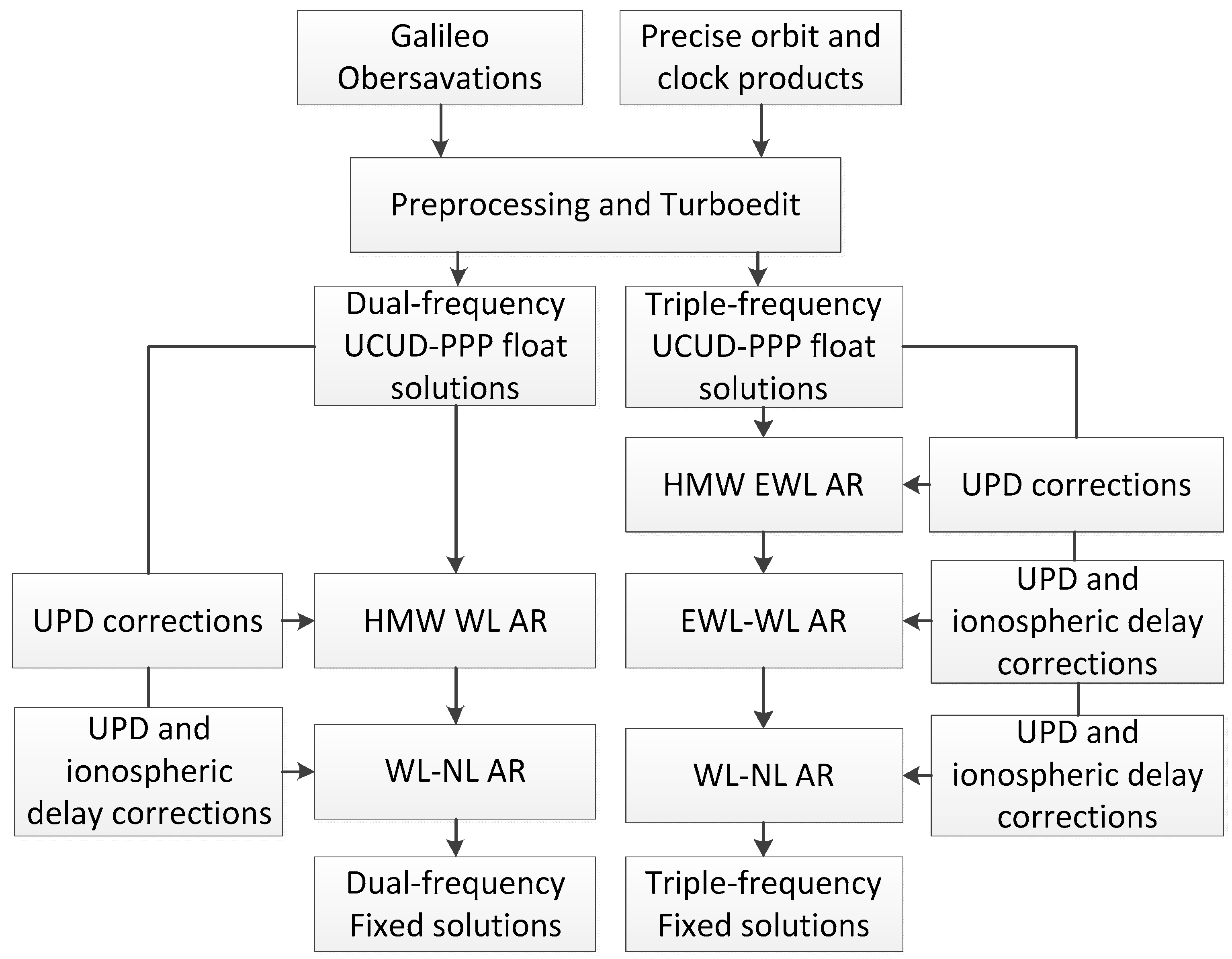
As shown in Figure 1, the main flows of dual- and triple-frequency UDUC-PPP AR are briefly summarized. As can be seen, Galileo observations and precise products are the prerequisite for both dual- and triple-frequency PPP. The data preprocessing and cycle slip detection are carried out before conducting PPP. Dual- or triple-frequency float solutions, including ionospheric delay information, can be easily obtained by the UDUC-PPP model. As we discussed above, dual- or triple-frequency AR can be sequentially resolved using the UPD product and ionospheric delay information. Except for taking advantage of additional observations, the benefit of triple-frequency AR lies in the EWL-WL AR which can weaken measurement noise compared with HMW WL AR.

3. Experiment and Results

In this section, experiments were carried out in order to validate the abovementioned method. We start with the estimating and discussing the characteristics of the Galileo UPDs, which is the prerequisite in precise point positioning with integer ambiguity resolution. Subsequently, we compare the performance of the dual- and triple-frequency float UDUC-PPP. Finally, for the sake of analyzing the benefits of AR using triple-frequency observations, we conduct a dual-frequency PPP AR which uses the WL-NL strategy and a triple-frequency PPP AR which uses the EWL-WL-NL strategy.

3.1. Data Processing Strategy and Original UPD Estimation

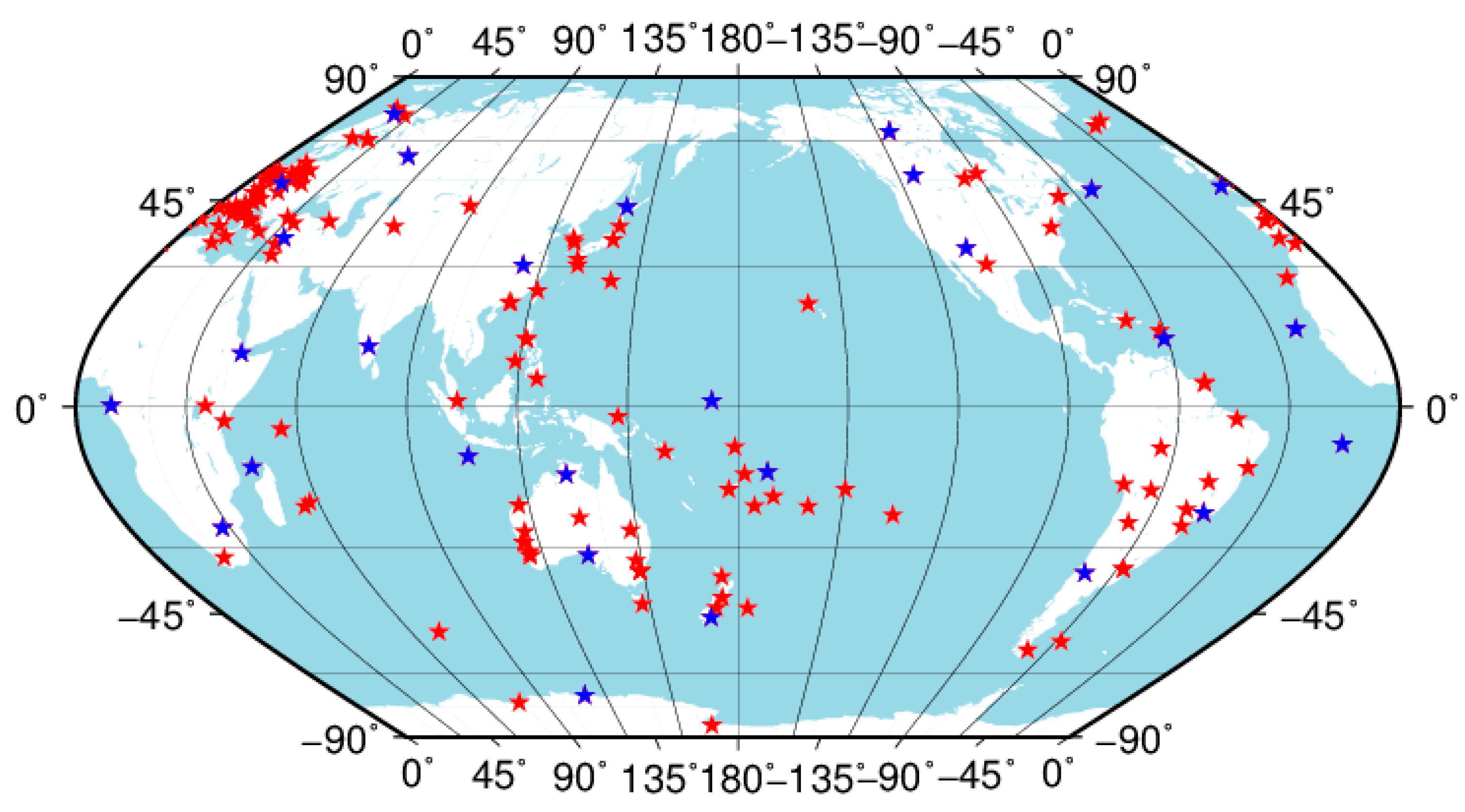
The estimation of UPD is the prerequisite in precise point positioning with integer ambiguity resolution. We use UDUC-PPP schemes to directly estimate the original UPD on each frequency from which we can easily form any combined UPDs, such as EWL and WL UPDs [19,21]. As shown in Figure 2, 166 Multi-GNSS Experiment (MGEX) stations with 30 s sampling interval observations are used for generating triple-frequency original UPDs and 28 stations are used for investigating the performance of UDUC-PPP. Weekly coordinate solutions in the SINEX format are used as the reference coordinates. As shown in

Table 1. The Galileo signal frequency and carrier-phase/pseudo-range observations.

GNSS System	Frequency (MHz)	Carrier Phase	Pseudo Range
	E1/1575.42	L1C/L1X	C1C/C1X
	E5a/1176.45	L5X/L5Q	C5X/C5Q
Galileo	E5b/1207.140	L7X/L7Q	C7X/C7Q
	E5/1191.795	L8X/L8Q	C8X/C8Q
	E6/1278.75	L6C/L6X	C6C/C6X

, the L1, L5 and L7 carrier-phase measurements are used with identical modulations for the pseudo-range measurements, which correspond to those in the E1, E5a and E5b bands, respectively. Carrier-phase observations are given a standard deviation of 3 millimeters, while code observations are de-weighted by a factor of 100 [29]. An elevation-angle-dependent weighting strategy also assigns lesser weight to satellites closer to the local horizon. Precise orbit and clock products at intervals of 5 min and 30 seconds, respectively, provided by GeoForschungsZentrum (GFZ), are used. The Galileo satellite PCO/PCV corrections are corrected with an IGS14 ANTEX file. Since there are no Galileo-specific station PCO/PCV corrections available, GPS values are used as approximations. More details about the Galileo UDUC-PPP processing strategy were summarized in

Table 2. The Galileo UDUC-PPP processing strategy.

Item	Strategies
Estimator	Sequential least square estimator
Observations	Original triple-frequency carrier-phase and pseudo-range observations
Signal selection	Galileo: E1/E5a/E5b
Sampling rate	30 s
Elevation cutoff	15°
Observations weight	Elevation-dependent weight
Ionospheric delay	Estimated as random-walk process
Tropospheric delay	Dry component: corrected with the Saastamoinen) model [30]
	Wet component: estimated as a random-walk process, a Global Mapping Function (GMF) mapping function
Receiver clock	Estimated as white noise
Station displacement	Corrected by IERS Convention 2010, including Solid Earth tide,
	pole tide and ocean tide loading [31]
Satellite PCO/PCV	Corrected using an IGS14 ANTEX file
Receiver PCO/PCV	Corrected using GPS values
Phase-windup effect	Corrected [32]
Relativistic effect	Applied
Station coordinate	Estimated as constants (Static PPP), a white noise (kinematic PPP)

.

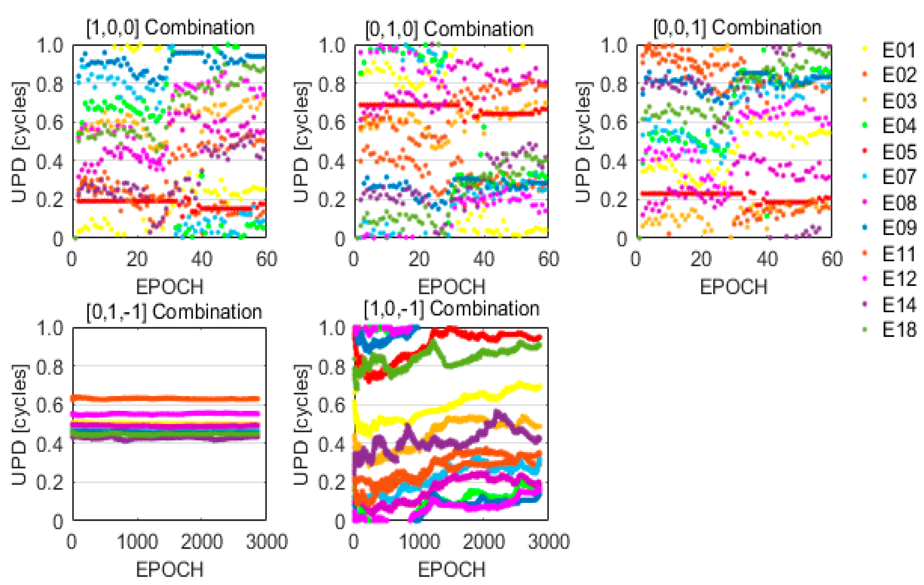
As shown in Figure 3 which depicts the fractional part of the Galileo satellite UPDs on DOY 201, 2018. (1, 0, 0), (0, 1, 0) and (0, 0, 1) UPDs denote the original UPDs on E1, E5a E5b signals, respectively. (0, 1, −1) and (1, 0, −1) UPDs denote the EWL and WL UPDs which could be easily obtained by linear combination of the original UPDs. In fact, original UPDs on each frequency have the advantage to allow for generating any kind of combined UPDs. As can be seen, the EWL UPDs are most stable throughout the whole day because of not only EWL ambiguities characterizing the long wavelength which is about 9.77 m but also EWL ambiguities getting rid of the geometry range as well as some atmosphere delay errors. Although WL ambiguities have similar characteristics as the EWL ambiguities, the relative short wavelength which is about 0.81 m is more easily impacted by measurement noise and multipath effects, which leads to the relative instability of WL UPDs. The original UPDs on each frequency are not stable because they cannot get rid of the impact of the geometry range as well as the atmosphere delay errors. Therefore, the original UPDs are more suitable to be estimated epoch-by-epoch, instead of establishing the forecasting model.

3.2. Performance Comparison of Dual- and Triple-Frequency Float PPP

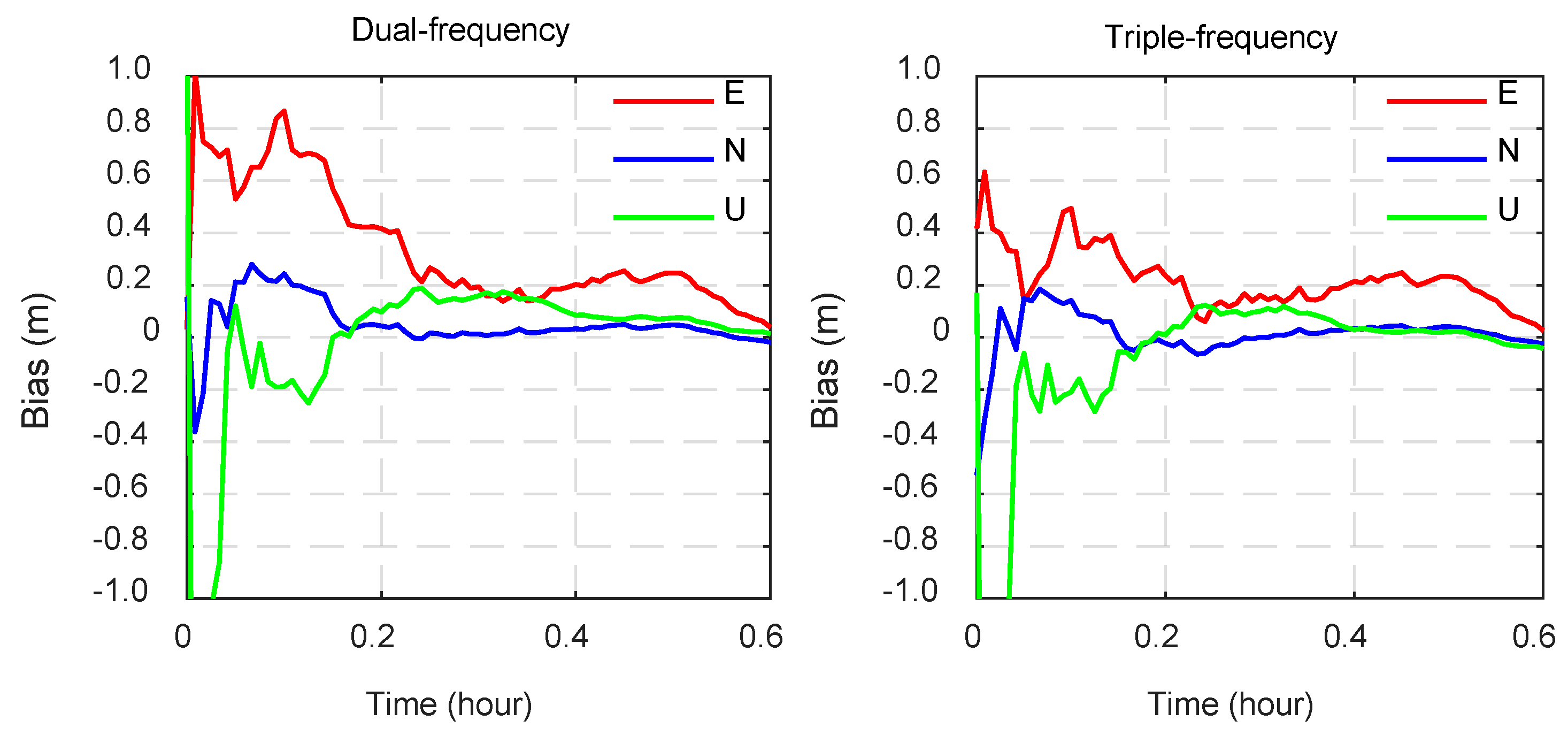
Figure 4 shows a typical time series of the position differences for the Galileo dual- and triple-frequency float PPPs at CPVG station during the initialization on DOY 201, 2018. As can be seen, the positioning accuracy of the triple-frequency PPP is significantly improved especially in the east direction during the first 12 min, even if only six Galileo satellites can be observed at the station. With only the one-epoch observation, the positioning accuracy of the triple-frequency PPP could reach to about 0.6 m in the east direction, in comparison to about a 1 m positioning accuracy of the dual-frequency PPP. With about 12-minute observations, the positioning accuracy of dual-frequency PPP in the east direction was about 0.4 m; however the positioning accuracy of the triple-frequency PPP was about 0.2 m in comparison, with the improvement by about 50%. Compared with dual-frequency observations, the triple-frequency observations surely improve significantly the positioning accuracy during the initial period.

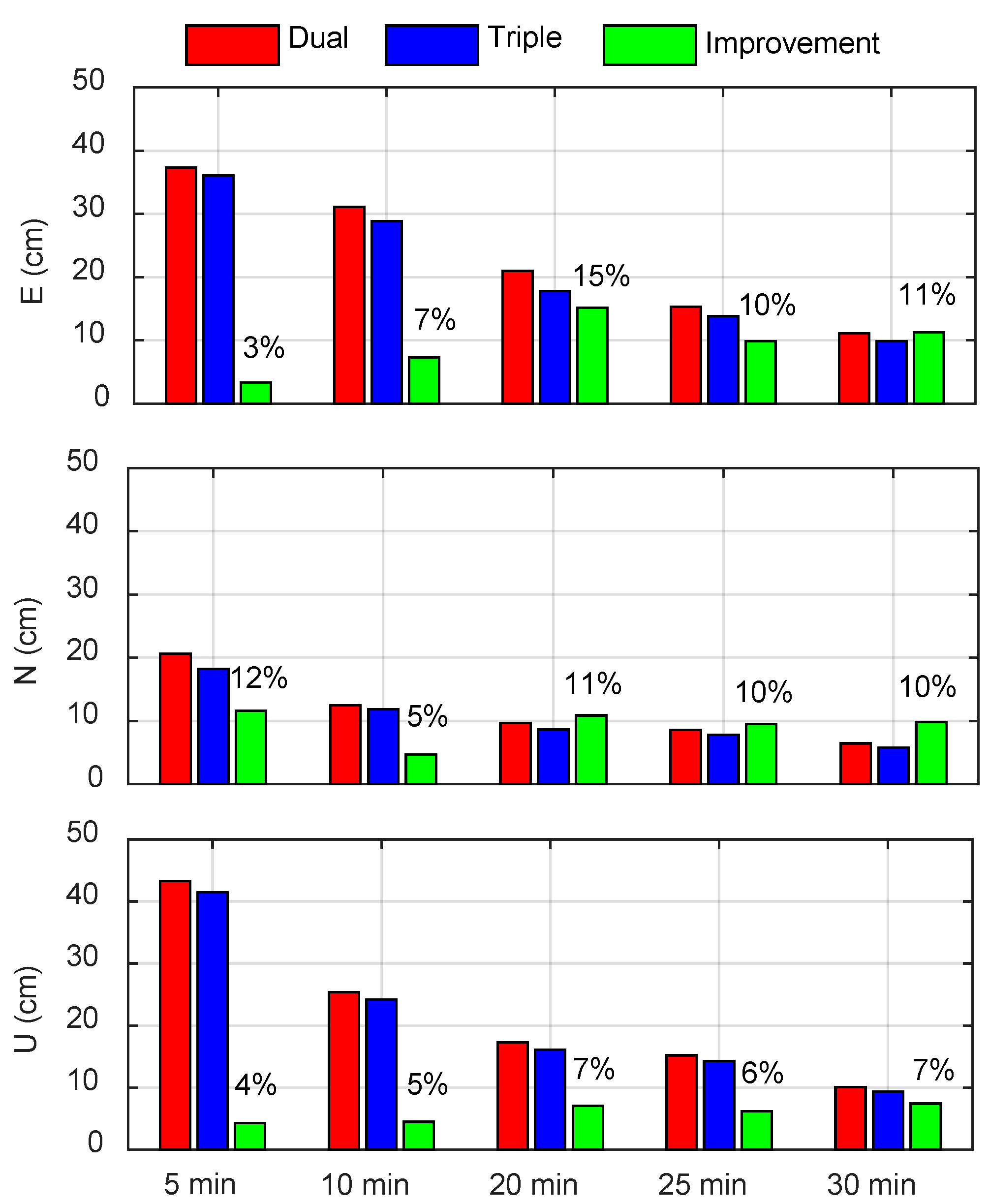
In order to further verify the improvement of convergence time using triple-frequency observations, the averaged positioning accuracy of all the test stations during the initialization was analyzed. In this study, the convergence time denoted the time when the positioning accuracy was better than 10 cm in successive five epochs. The statistics showed averaged positioning accuracy for each session of 5, 10, 20, 25 and 30 min, as shown in Figure 5. As can be seen, the positioning accuracy could be improved in the east, north and up directions when using triple-frequency observations in each session. During the period of 20–30 min, the improvement of the positioning accuracy was the most significant, with about 10–15% in the horizontal direction and 6–7% in the vertical direction. The averaged convergence time for the current Galileo triple-frequency float PPP was about 30 min, with the improvement of about 10% compared with dual-frequency float PPP. It concludes that the additional observations are helpful to improve the performance of float PPP in terms of convergence time and positioning accuracy.

3.3. Performance Comparison of Dual- and Triple-Frequency PPP AR

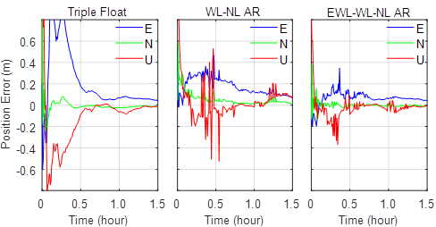
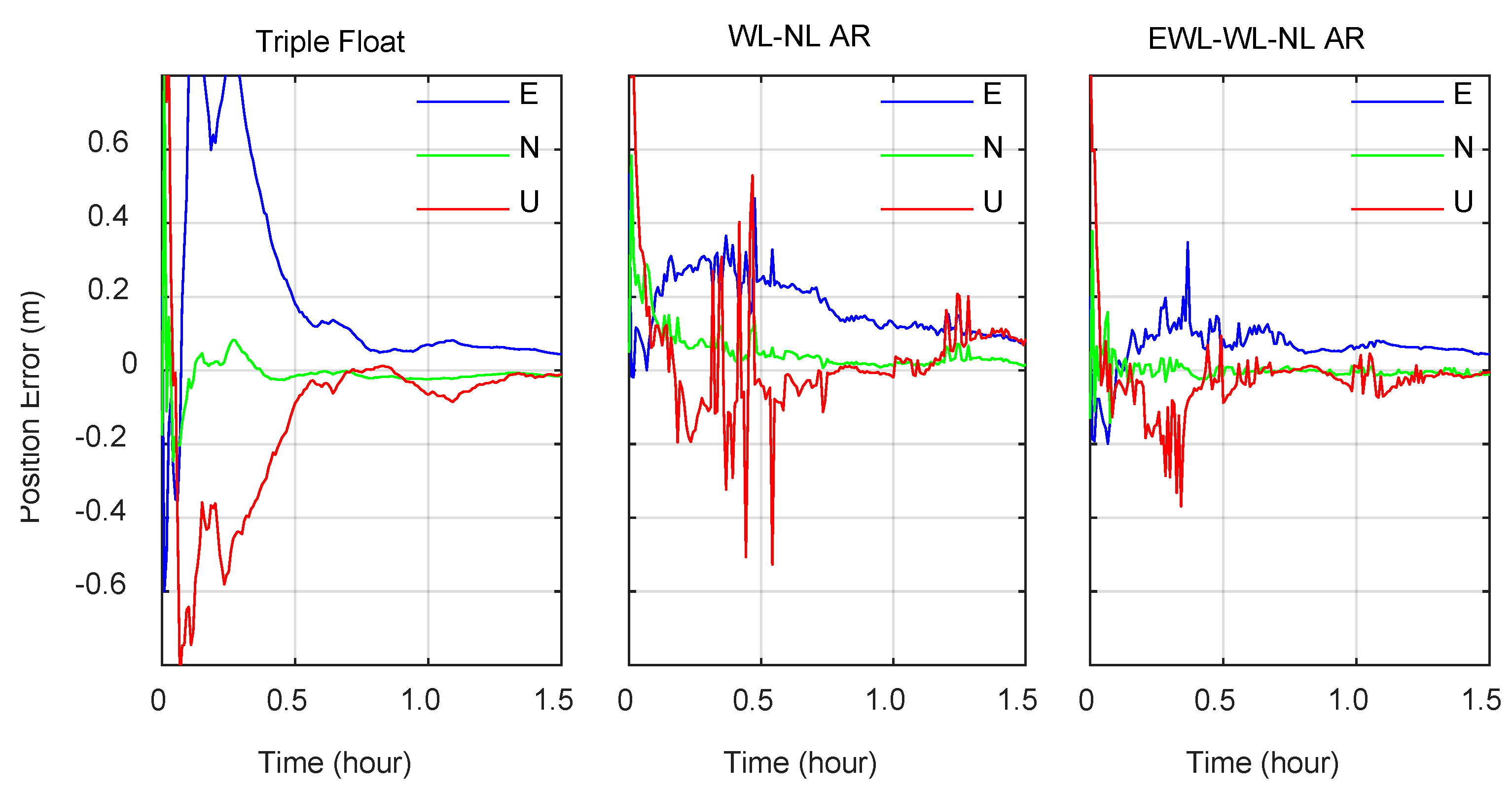
Figure 6 shows the typical position differences for the triple-frequency float solutions, dual-frequency WL-NL AR and triple-frequency EWL-WL-NL AR, making the results with 1.5-h observations at ASCG station on DOY 201, 2018. Because it is expected that not all ambiguities can be fixed simultaneously, a partial ambiguity resolution scheme was conducted [33,34]. As can be seen, the convergence trend of PPP AR, especially triple-frequency PPP AR which had the potential for significantly precise instantaneous positioning, was obviously much faster than the triple-frequency float PPP during the period of the initial ten minutes. Compared with the dual-frequency WL-NL AR, the triple-frequency EWL-WL-NL AR obviously reduced the convergence time and also improved the positioning accuracy. The obtained positioning accuracy of the triple-frequency EWL-WL-NL AR was about 0.2 m instantaneously and dropped down to 0.1 m after 0.5 h of observation time. However, the dual-frequency WL-NL AR reached 0.1 m with about 0.8-h of observations. In addition, during the initialization, especially in the initial 10─30 min, the positioning difference of the triple-frequency EWL-WL-NL AR was more stable than that of the dual-frequency WL-NL AR. The reason may be the difference of the WL ambiguity resolution between dual- and triple-frequency AR. Using the EWL-WL strategy with a ten times smaller measurement noise than the HMW combination WL strategy allows us to successfully resolve the WL ambiguity more easily and rapidly.

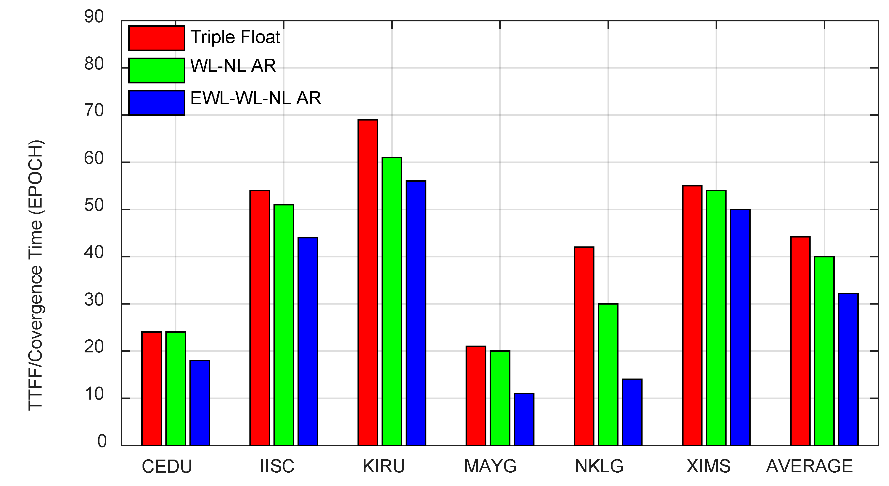
For the purpose of assessing the performance of UDUC-PPP AR further, the TTFF of the dual- and triple-frequency AR as well as the convergence time of the triple-frequency float solutions at the six user stations are shown in Figure 7. The averaged convergence time and TTFF for three groups of solutions are also depicted in Figure 7. In this study, the TTFF denoted the time when the posterior positioning accuracy was in centimeter levels in successive five epochs. It can be demonstrated that the TTFF of the triple-frequency AR is shorter than that of the dual-frequency AR and also shorter than the convergence time of the triple-frequency float PPP at different user stations. The improvement of TTFF varied at different stations. This variation depends on many factors such as latitude, atmosphere condition and receiver types, which need to be studied further. On average, the results of the six stations showed that the TTFF of the triple-frequency AR was about 32 epochs (16 min), which reduced the TTFF by 19.6% compared with the dual-frequency AR and also reduced the convergence time by 27.2% compared with the triple-frequency float PPP.

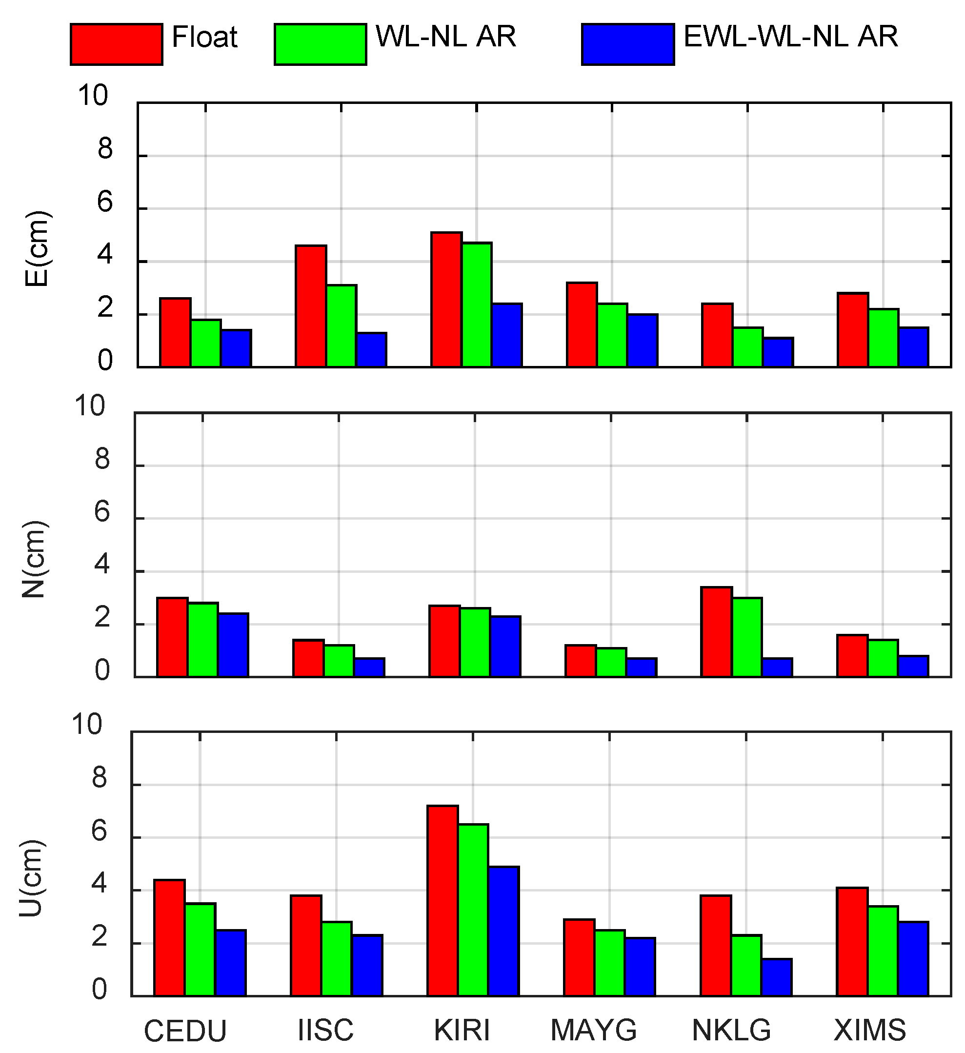
In order to study the positioning accuracy of UDUC-PPP AR, the positioning differences of the triple-frequency float solutions, dual-frequency WL-NL AR and triple-frequency EWL-WL-NL AR with 2-h observations were calculated at the six user stations, as shown in Figure 8. One can see that the current triple-frequency Galileo positioning accuracy with 2-h observations could reach up to 2–4 cm in the east direction, 1–3 cm in the north direction and 2–7 cm in the up direction. It could be seen that the positioning accuracy of the triple-frequency AR was the highest compared with the dual-frequency AR and triple-frequency float solutions. On average,

Table 3. The RMS of the positioning errors for three groups of PPP solutions with 2-h observations for all test stations (unit: cm).

	Triple Float	WL-NL AR	EWL-WL-NL AR
E	0.36	0.28	0.17
N	0.24	0.21	0.15
U	0.46	0.38	0.29

shows the root mean square (RMS) of positioning errors with 2-h observations for the dual-frequency and triple-frequency AR, as well as the triple-frequency float solutions. As can be seen, the triple-frequency PPP AR improved the averaged positioning accuracy by 40.9%, 31.2% and 23.6% compared with the dual-frequency PPP AR and 53.3%, 37.6% and 36.8% compared with the triple-frequency float solutions, in the east, north and up directions, respectively.

4. Discussion

Multi-frequency GNSS PPP-AR is the future direction. In this paper, we verified the triple-frequency UDUC-PPP AR using the Galileo observations provided by IGS-MGEX stations. The averaged statistics demonstrated that the TTFF of Galileo triple-frequency PPP AR was about 32 epochs (16 min), which reduced the TTFF by 19.6% compared with the Galileo dual-frequency PPP AR and also reduced the convergence time by 27.2% compared with the Galileo triple-frequency float PPP. The Galileo triple-frequency PPP AR improved the averaged positioning accuracy by 40.9%, 31.2% and 23.6% compared with the Galileo dual-frequency PPP AR and 53.3%, 37.6% and 36.8% compared with the Galileo triple-frequency float PPP, in the east, north and up directions, respectively. Our statistics about the contribution of triple-frequency observations were much better than those reported by Gu et al. [20] and Li et al. [21]. The reasons may be the fact that not only the precise orbits and clock products of the Galileo satellites but also the PCO/PCV corrections of the Galileo satellites are more accurate than that of the BDS satellites.

As shown in Figure 6, although the triple-frequency AR has great potential to achieve instantaneous centimeter-level precise point positioning, there are still many challenges. As discussed above, there are two main factors that influence rapid PPP AR: measurement noise and residual errors of ionospheric delay. Compared with reducing ionospheric errors, measurement noise processing is more complex. There is no better way to deal with measurement noise but multi-epoch smoothing, which is an important factor limiting rapid PPP AR. Compared to the HMW combination strategy for dual-frequency WL AR, the EWL-WL strategy for triple-frequency WL AR greatly reduces the measurement noise which is the main reason to improve TTFF. As can be seen in Figure 7 and Figure 8, the improvement of the performance of triple-frequency AR is different in each station, which is mainly due to the difference of the ionospheric delay corrections, estimated by the UDUC-PPP model. Due to the current number of Galileo satellites, the accuracy of the ionospheric delay estimates based on the UDUC-PPP model is still limited, leading to unstable positioning results of the triple-frequency AR, as shown in Figure 6.

5. Conclusions

As the number of Galileo satellites increases, we can take advantage of the Galileo constellation to conduct multi-frequency PPP AR. In order to verify that extra frequency signals can contribute to the performance of UDUC-PPP AR, this paper proposed the method of a multi-frequency step-by-step AR suitable for dual- and triple-frequency data processing, based on the UDUC-PPP model. The experiment results showed that the triple-frequency UDUC-PPP can be conducted with a significant improvement in terms of positioning accuracy and convergence time compared with dual-frequency PPP. The triple-frequency float PPP could contribute to improving the position estimations especially during the initialization phase. The averaged convergence time for the current Galileo triple-frequency float PPP was about 30 min, with the improvement of about 10%, compared with the dual-frequency float PPP. Compared with the dual-frequency WL-NL AR, triple-frequency EWL-WL-NL AR could obviously reduce the TTFF and also improve the positioning accuracy.

In addition, we also discussed the reasons why triple-frequency AR is more rapid than dual-frequency AR. The main difference between the dual-frequency AR and triple-frequency AR lies in the way the WL ambiguity is resolved. Using the cascaded strategy of EWL-WL for triple-frequency AR, which goes with ten times smaller measurement noise than the HMW combination WL strategy for dual-frequency, allows the WL ambiguity to be successfully resolved more easily and rapidly. Although the performance of the UDUC-PPP AR can be improved using triple-frequency observations, the accuracy of the ionospheric delay estimates is still a main factor which limits the instantaneous ambiguity resolution. We expect to improve the accuracy of ionospheric delay estimates through multi-GNSS and multi-frequency technology which can further improve the TTFF and the positioning accuracy of UDUC-PPP AR.

References

- Bisnath, S.; Gao, Y. Current State of Precise Point Positioning and Future Prospects and Limitations. Int. Assoc. Geod. Symp. 2008, 133, 615–623. [Google Scholar]
- Ge, M.; Gendt, G.; Rothacher, M.; Shi, C.; Liu, J. Resolution of GPS carrier-phase ambiguities in Precise Point Positioning (PPP) with daily observations. J. Geod. 2008, 82, 389–399. [Google Scholar] [CrossRef]
- Collins, P.; Bisnath, S.; Lahaye, F.; Héroux, P. Undifferenced GPS Ambiguity Resolution Using the Decoupled Clock Model and Ambiguity Datum Fixing. J. Inst. Navig. 2010, 57, 123–135. [Google Scholar] [CrossRef]
- Laurichesse, D.; Mercier, F.; Berthias, J.-P.; Broca, P.; Cerri, L. Integer Ambiguity Resolution on Undifferenced GPS Phase Measurements and Its Application to PPP and Satellite Precise Orbit Determination. J. Inst. Navig. 2009, 56, 135–149. [Google Scholar] [CrossRef]
- Li, X.; Ge, M.; Dousa, J.; Wickert, J. Real-time precise point positioning regional augmentation for large GPS reference networks. GPS Solut. 2013, 18, 61–71. [Google Scholar] [CrossRef]
- Forssell, B.; Martin-Neira, M.; Harrisz, R.A. Carrier phase ambiguity resolution in GNSS-2. In Proceedings of the 10th International Technical Meeting of the Satellite Division of the Institute of Navigation (ION GPS 1997), Kansas, MO, USA, 16–19 September 1997; pp. 1727–1736. [Google Scholar]
- Vollath, U.; Birnbach, S.; Landau, H.; Fraile-Ordoñez, J.M.; Martin-Neira, M. Analysis of Three-Carrier Ambiguity Resolution (TCAR) Technique for Precise Relative Positioning in GNSS-2. In Proceedings of the 11th International Technical Meeting of the Satellite Division of The Institute of Navigation (ION GPS 1998), Nashville, TN, USA, 15–18 September 1998; pp. 417–426. [Google Scholar]
- De Jonge, P.; Teunissen, P.; Jonkman, N.; Joosten, P. The distributional dependence of the range on triple frequency GPS ambiguity resolution. In Proceedings of the National Technical Meeting of The Institute of Navigation, Anaheim, CA, USA, 26–28 January 2000; Volume 5, pp. 605–612. [Google Scholar]
- Hatch, R.; Jung, J.; Enge, P.; Pervan, B. Civilian GPS: The Benefits of Three Frequencies. GPS Solut. 2000, 3, 1–9. [Google Scholar] [CrossRef]
- Werner, W.; Winkel, J. TCAR and MCAR options with Galileo and GPS. In Proceedings of the 16th International Technical Meeting of the Satellite Division of The Institute of Navigation (ION GPS/GNSS), Portland, OR, USA, 9–12 September 2003; pp. 790–800. [Google Scholar]
- Feng, Y. GNSS three carrier ambiguity resolution using ionosphere-reduced virtual signals. J. Geod. 2008, 82, 847–862. [Google Scholar] [CrossRef]
- Li, B.; Feng, Y.; Shen, Y. Three carrier ambiguity resolution: distance-independent performance demonstrated using semi-generated triple frequency GPS signals. GPS Solut. 2009, 14, 177–184. [Google Scholar] [CrossRef]
- Tang, W.; Deng, C.; Shi, C.; Liu, J. Triple-frequency carrier ambiguity resolution for Beidou navigation satellite system. GPS Solut. 2013, 18, 335–344. [Google Scholar] [CrossRef]
- Zhao, Q.; Dai, Z.; Hu, Z.; Sun, B.; Shi, C.; Liu, J. Three-carrier ambiguity resolution using the modified TCAR method. GPS Solut. 2014, 19, 589–599. [Google Scholar] [CrossRef]
- Zhang, X.; He, X. Performance analysis of triple-frequency ambiguity resolution with BeiDou observations. GPS Solut. 2015, 20, 269–281. [Google Scholar] [CrossRef]
- Geng, J.; Bock, Y. Triple-frequency GPS precise point positioning with rapid ambiguity resolution. J. Geod. 2013, 87, 449–460. [Google Scholar] [CrossRef]
- Liu, T.; Wang, N.; Tan, B.; Chen, Y.; Yuan, Y.; Zhang, B. Multi-GNSS precise point positioning (MGPPP) using raw observations. J. Geod. 2016, 91, 253–268. [Google Scholar] [CrossRef]
- Wang, K.; Khodabandeh, A.; Teunissen, P.J.G. Five-frequency Galileo long-baseline ambiguity resolution with multipath mitigation. GPS Solut. 2018, 22, 75. [Google Scholar] [CrossRef]
- Odijk, D.; Zhang, B.; Khodabandeh, A.; Odolinski, R.; Teunissen, P.J.G. On the estimability of parameters in undifferenced, uncombined GNSS network and PPP-RTK user models by means of S-system theory. J. Geod. 2016, 90, 15–44. [Google Scholar] [CrossRef]
- Gu, S.; Lou, Y.; Shi, C.; Liu, J. BeiDou phase bias estimation and its application in precise point positioning with triple-frequency observable. J. Geod. 2015, 89, 979–992. [Google Scholar] [CrossRef]
- Li, P.; Zhang, X.; Ge, M.; Schuh, H. Three-frequency BDS precise point positioning ambiguity resolution based on raw observables. J. Geod. 2018, 92, 1357–1369. [Google Scholar] [CrossRef]
- Teunissen, P.J.G. The least-squares ambiguity decorrelation adjustment: a method for fast GPS integer ambiguity estimation. J. Geod. 1995, 70, 65–82. [Google Scholar] [CrossRef]
- Zhang, B.; Chen, Y.; Yuan, Y. PPP-RTK based on undifferenced and uncombined observations: theoretical and practical aspects. J. Geod. 2018, 1–14. [Google Scholar] [CrossRef]
- Teunissen, P.J.G.; Joosten, P.; Tiberius, C. A comparison of TCAR, CIR and LAMBDA GNSS ambiguity resolution. In Proceedings of the 15th International Technical Meeting of the Satellite Division of the Institute of Navigation (ION GPS 2002), Portland, OR, USA, 24–27 September 2002; pp. 2799–2808. [Google Scholar]
- Guo, F.; Zhang, X.; Wang, J.; Ren, X. Modeling and assessment of triple-frequency BDS precise point positioning. J. Geod. 2016, 90, 1223–1235. [Google Scholar] [CrossRef]
- Hatch, R. The synergism of GPS code and carrier measurement. In Proceedings of the Third International Geodetic Symposium Satellite Doppler Positioning, La Cruces, NM, USA, 8–12 February 1982; pp. 1213–1232. [Google Scholar]
- Melbourne, W.G. The Case for Ranging in GPS-based Geodetic Systems. In Proceedings of the 1st International Symposium on Precise Positioning with the Global Positioning System, Rockville, MD, USA, 15–19 April 1985; pp. 373–386. [Google Scholar]
- Wübbena, G. Software Developments for Geodetic Positioning with GPS using TI-4100 Code and Carrier Measurements. In Proceedings of the 1st International Symposium on Precise Positioning with the Global Positioning System, Rockville, MD, USA, 15–19 April 1985; pp. 403–412. [Google Scholar]
- Innovation: Instantaneous Centimeter-Level Multi-Frequency Precise Point Positioning. Available online: https://www.gpsworld.com/innovation-instantaneous-centimeter-level-multi-frequency-precise-point-positioning/ (accessed on 6 February 2019).
- Saastamoinen, J. Contributions to the theory of atmospheric refraction – Part II. Refraction corrections in satellite geodesy. Bull. Géod. 1973, 47, 13–34. [Google Scholar] [CrossRef]
- Petit, G.; Luzum, B. IERS Conventions (2010); IERS technical note No. 36; Publisher of the Federal Agency for Cartography and Geodesy: Frankfurt am Main, Germany, 2010; p. 179. [Google Scholar]
- Wu, J.T.; Wu, S.C.; Hajj, G.A.; Bertiger, W.I.; Lichten, S.M. Effects of antenna orientation on GPS carrier phase. Manuscr. Geod. 1993, 18, 91–98. [Google Scholar]
- Wang, J.; Feng, Y. Reliability of partial ambiguity fixing with multiple GNSS constellations. J. Geod. 2012, 87, 1–14. [Google Scholar] [CrossRef]
- Li, P.; Zhang, X. Precise Point Positioning with Partial Ambiguity Fixing. Sensors 2015, 15, 13627–13643. [Google Scholar] [CrossRef] [PubMed]
Figure 1.
A flowchart of the dual- and triple-frequency un-differenced and uncombined precise point positioning (UCUD-PPP) ambiguity resolution.
Figure 2.
The distribution of the Galileo reference network and user stations. The red stars denote the reference stations for estimating the uncalibrated phase delays (UPDs); the blue stars denote the user stations for testing the performance of PPP.
Figure 3.
The time series of UPDs for each epoch on day of year (DOY) 201, 2018. (1, 0, 0), (0, 1, 0) and (0, 0, 1) UPD denote the original UPDs of Galileo E1, E5a and E5b signals, respectively. (0, 1, −1) and (1, 0, −1) denote Galileo EWL and WL UPDs.
Figure 4.
The time series of the position differences for the dual-frequency and triple-frequency float solutions with 0.6-h observations at CPVG station on DOY 201, 2018.
Figure 5.
The averaged positioning errors of all the test stations in the east, north and up components for dual-frequency and triple-frequency float solutions during the initialization on DOY 201, 2018.
Figure 6.
The time series of the position differences for the triple-frequency float solutions, dual-frequency WL-NL AR and triple-frequency EWL-WL-NL AR with 1.5-h observations at ASCG station on DOY 201, 2018.
Figure 7.
The time-to-first-fix (TTFF) of the dual-frequency AR and triple-frequency AR, as well as the convergence time of the triple-frequency float solutions at the user stations on DOY 201, 2018.
Figure 8.
The RMS of the positioning errors with a 2-h observation for the dual-frequency and triple-frequency AR, as well as the triple-frequency float solutions (unit: cm).