Exploring the Potential of Satellite Solar-Induced Fluorescence to Constrain Global Transpiration Estimates

Abstract

The opening and closing of plant stomata regulates the global water, carbon and energy cycles. Biophysical feedbacks on climate are highly dependent on transpiration, which is mediated by vegetation phenology and plant responses to stress conditions. Here, we explore the potential of satellite observations of solar-induced chlorophyll fluorescence (SIF)—normalized by photosynthetically-active radiation (PAR)—to diagnose the ratio of transpiration to potential evaporation (‘transpiration efficiency’, τ). This potential is validated at 25 eddy-covariance sites from seven biomes worldwide. The skill of the state-of-the-art land surface models (LSMs) from the eartH2Observe project to estimate τ is also contrasted against eddy-covariance data. Despite its relatively coarse (0.5°) resolution, SIF/PAR estimates, based on data from the Global Ozone Monitoring Experiment 2 (GOME-2) and the Clouds and Earth’s Radiant Energy System (CERES), correlate to the in situ τ significantly (average inter-site correlation of 0.59), with higher correlations during growing seasons (0.64) compared to decaying periods (0.53). In addition, the skill to diagnose the variability of in situ τ demonstrated by all LSMs is on average lower, indicating the potential of SIF data to constrain the formulations of transpiration in global models via, e.g., data assimilation. Overall, SIF/PAR estimates successfully capture the effect of phenological changes and environmental stress on natural ecosystem transpiration, adequately reflecting the timing of this variability without complex parameterizations.

1. Introduction

Plant transpiration dominates the global flux of terrestrial evaporation and is a central element of the hydrologic cycle over land [1,2]. The transpiration flux depends on plant phenology and is mediated by stomatal conductance, by which plants tend to optimize to maximize carbon uptake while reducing water losses [3,4,5,6]. As such, the biophysical and biochemical feedbacks on climate depend on vegetation phenology and plant physiological response to environmental conditions and nutrient cycling [7,8,9,10]. These responses vary among plant species and make the modelling of transpiration particularly challenging [11,12,13]. More specifically, the physiological response to water stress remains a longstanding modelling challenge [14], which may ultimately be addressed by incorporating plant hydraulics into land surface models (LSMs) [15,16,17].

However, perhaps unsurprisingly, current LSMs still constrain transpiration based on empirical relationships between stomatal conductance and environmental variables such as soil moisture, temperature and vapor pressure deficit [18,19,20]. These formulations are supported by limited observational evidence at global scales, and their assumptions affect the modelled heat and drought response of ecosystem transpiration, which remains uncertain in current models [7,21,22]. The effect of water stress on transpiration is typically introduced in LSMs through a dimensionless empirical factor based on an assumed relationship between soil moisture and stomatal conductance, net photosynthesis, mesophyll conductance and/or carboxylation rate [21,23,24,25]. Pure hydrologic and remote-sensing models—which have no explicit photosynthesis and coupled stomatal dependence—use similar empirical water-stress functions to constrain the potential transpiration estimates from Penman–Monteith or Priestley and Taylor approaches [26,27,28,29,30]. Two-source energy balance models utilize remotely sensed surface temperatures to constrain transpiration, but often still rely on Penman–Monteith, Priestley and Taylor, or aerodynamic formulations [31], or solve for latent heat as the residual term in the energy balance [32,33].

Given (a) the importance of transpiration for global hydrology and climate, (b) the dependency of transpiration on phenology and physiological response to environmental stress, and (c) the difficulties representing this response in models, there is a need to unravel these processes at a global scale from an observational perspective. Due to the scarcity and limited coverage of in situ observations, satellite retrievals appear as an attractive means to monitor transpiration constraints, unravel the implications in terms of land feedbacks on climate, and improve the representation of transpiration in LSMs. However, current efforts to study transpiration dynamics based on satellite data are hampered by the inability to detect this flux directly from space [13,34] and are thus limited to process-based modelling [35,36] or machine-learning algorithms [37] run with observed environmental drivers of the flux. Moreover, even when these methods estimate the total terrestrial evaporation reliably, the transpiration component of the flux remains highly uncertain [35,38].

Solar-induced chlorophyll fluorescence (SIF) is a byproduct of photosynthesis: a small fraction of light, initially absorbed by chlorophyll pigments, that is re-emitted as a subtle glow of energy in the spectral range of 650–800 nm [39,40]. The intensity of the SIF signal is indicative of the functioning of the photosynthetic machinery [41]. As water lost through transpiration and carbon uptake through photosynthesis is synchronized by stomatal opening, and is sensitive to similar environmental drivers, negative anomalies in SIF are expected to integrate the effects of different environmental stressors on transpiration [42,43,44]. Spaceborne datasets of global SIF have become available in recent years [45,46,47,48,49,50]. These datasets are already being used to monitor crop photosynthetic activity and gross primary production (GPP) [51,52,53], estimate surface turbulent fluxes [42,54], and improve LSM estimates of photosynthesis [55,56]. However, their potential to understand the effects of environmental stress on global transpiration has not been evaluated.

Here, we present a novel application of SIF observations to diagnose transpiration efficiency (τ), understood as the ratio between transpiration (T) and potential evaporation (E_p). We also establish an in situ validation dataset of τ across eddy-covariance sites to test the performance of satellite retrievals. Analogous τ estimates from a set of four offline LSMs, one hydrologic model and one transpiration retrieval model from the eartH2Observe database [57] (see Section 2.4) are compared against in situ and satellite retrievals. This is done with the ultimate goal to evaluate the potential of SIF to benchmark the representation of transpiration in traditional LSMs.

2. Materials and Methods

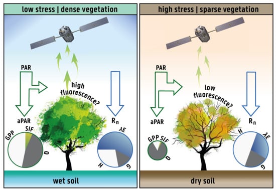
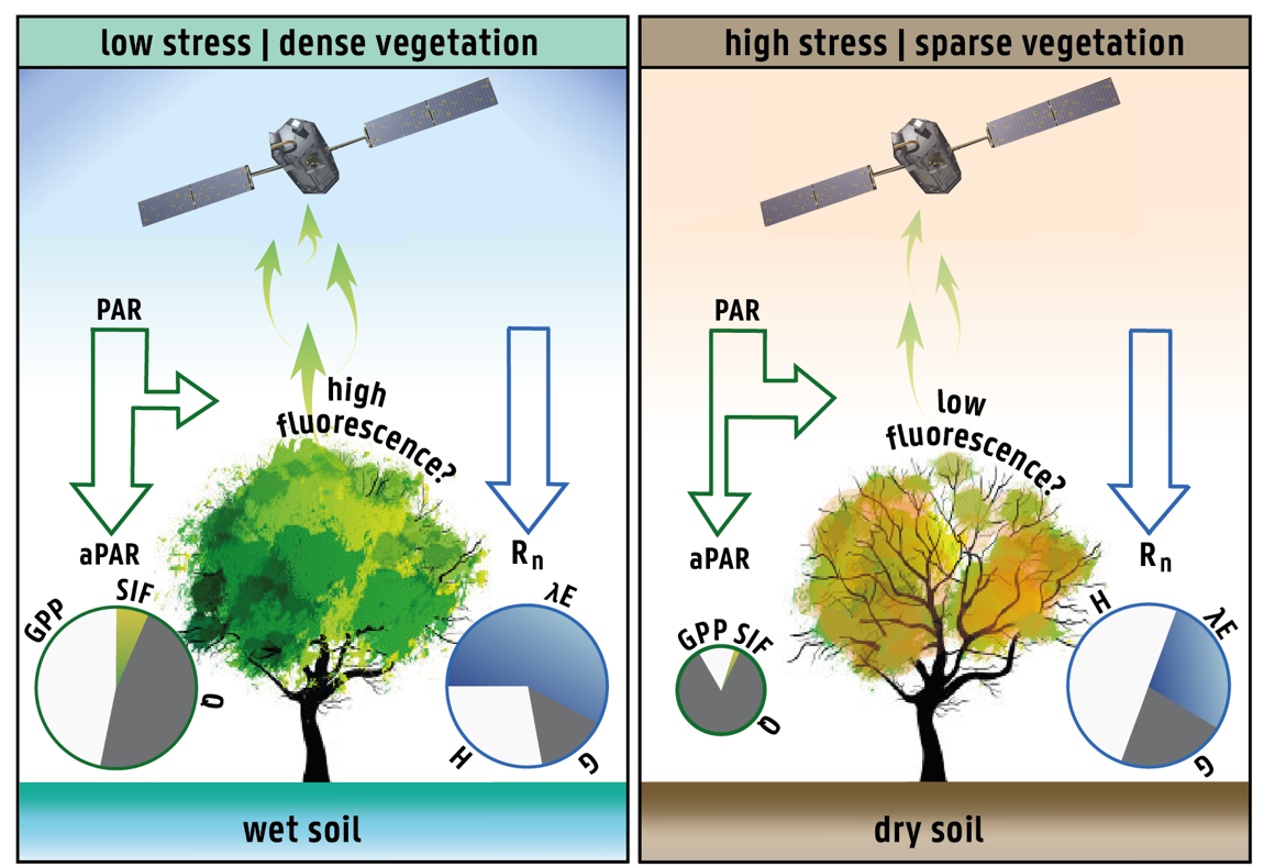
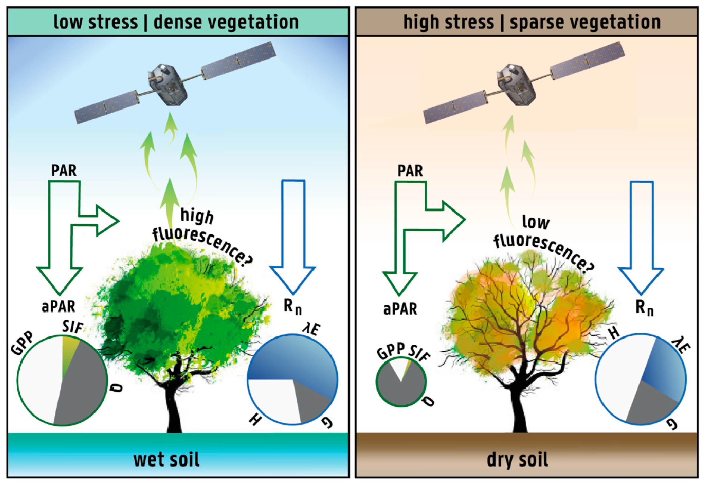
2.1. Rationale and Hypothesis

To date, several studies have suggested a near-linear proportional relationship between GPP and SIF over temporal scales larger than daily [48,58,59]. Since stomatal opening regulates both the CO₂ uptake and vapour loss through transpiration, SIF may also be of use to diagnose transpiration [42,44,60]. From that rationale, it follows that transpiration (T) and SIF hold a proportional relationship that is mediated by the ecosystem water-use efficiency (WUE):

$$\mathrm{T}\propto \mathrm{SIF}\times \mathrm{WUE}$$

(1)

where WUE reflects the ratio of GPP to T. While in nature WUE depends on a plethora of factors, it is widely acknowledged that the atmospheric demand for water explains a large fraction of its variability at ecosystem scale [44,61]: under conditions of high potential evaporation (E_p), the water loss per unit gain of carbon increases. As such, here we explore whether the fraction of E_p that is transpired (hereafter referred to as ‘transpiration efficiency’, τ) holds a proportional relationship to the fraction of photosynthetically active radiation (PAR) that is emitted as SIF:

$$\mathsf{\tau }=\frac{\mathrm{T}}{{\mathrm{E}}_{\mathrm{p}}}\propto \frac{\mathrm{SIF}}{\mathrm{PAR}}$$

(2)

The normalization of SIF (mW/m²/sr/nm) by PAR (W/m²) allows the correction of incoming radiation changes—independent of phenological variability or physiological stress [62]—in an analogous way that the normalization of T by E_p buffers the effect of short-term changes in available energy. Moreover, normalizing by PAR intentionally retains the variability in SIF associated with changes in the fraction of absorbed PAR (i.e., fPAR), which allows us to employ an analogous E_p calculation that is merely atmospheric, so that τ reflects the limitations of the actual ecosystem in response to the atmospheric demand for water (whether that ecosystem limitation has a structural or physiological origin). Following the findings in Maes et al. [63], in which multiple E_p equations were evaluated, E_p (W/m²) is calculated here based on the simple radiation-based formulation by Milly and Dunne [64]:

$${\mathrm{E}}_{\mathrm{p}}=\mathsf{\alpha }\left({\mathrm{R}}_{\mathrm{n}}-\mathrm{G}\right)$$

(3)

where α is a constant unitless parameter (similar to α in the Priestley and Taylor equation), R_n (W/m²) is the surface net radiation and G (W/m²) is the ground heat flux. Maes et al. [63] recommended using a biome-specific parameterization of α rather than the universal value of α = 0.8 proposed by Milly and Dunne [64]—see Table S1 for specific values of α per biome type.

The rationale behind the hypothesis confined in Equation (2) is illustrated in Figure 1. Given a certain amount of R_n and PAR, under low stress conditions (and/or high leaf area), we expect higher levels of transpiration (i.e., λE), GPP and SIF than under high stress conditions (and/or low leaf area) given the same R_n and PAR. For the latter, we expect more sensible heat flux (H), non-radiative decay and non-photochemical quenching (Q). This hypothesis is further sustained by the results from Maes et al. [65], which, by employing an advanced radiative transfer model, showed that most of the variance in T that is left unexplained by SIF variability can be explained by changes in the atmospheric potential to evaporate water.

2.2. Satellite Observations

SIF observations are taken from the Global Ozone Monitoring Experiment-2 (GOME-2) on-board EUMETSAT’s Meteorological Operational Satellite-A (MetOp-A) for the time period 2007–2014. These retrievals are based on the method by Köhler et al. [47], and are obtained from the band 4 using a spectral window of 720–758 nm. Data is available globally at 0.5° spatial resolution and up to 1.5-day temporal resolution in the absence of clouds. SIF data is taken from GOME-2 rather than newer sensors, such as the Orbiting Carbon Observatory-2 (OCO-2) or the TROPOspheric Monitoring Instrument (TROPOMI), as GOME-2 has global coverage and the longest record length. PAR data from the Clouds and Earth’s Radiant Energy System (CERES) [66] are selected based on the closest overpass time to GOME-2 (near 9:30AM), and resampled from 1° to 0.5°. SIF and PAR retrievals are cross-masked and temporally gap-filled prior to the calculation of their ratio using a 15-day moving window; when necessary, estimates are subsequently spatially gap-filled by weighting the eight neighboring pixels based on distance. Time steps with PAR < 40 W/m² are masked to exclude potential nighttime conditions in high latitudes. Finally, GLOBSNOW snow water equivalent data [67] is used to mask for snow conditions.

2.3. Tower Data

Data from the FLUXNET2015 archive of eddy-covariance tower measurements (http://fluxnet.fluxdata.org/data/fluxnet2015-dataset/) are used to create an in situ τ validation dataset by computing the ratio between transpiration and potential evaporation at each daily time step for each tower using daytime values. The measured latent heat at each tower is partitioned into transpiration and soil evaporation using the simple approach introduced by Wei et al. [1], where the ratio of T to total evaporation is a function of land cover type and leaf area index (LAI)—the latter is obtained from the Global Inventory Modeling and Mapping Studies (GIMMS) [68,69]. Using the empirical equations provided by Wei et al. [1], International Geosphere-Biosphere Programme (IGBP) classifications are regrouped into six categories, and the ratio of T to total evaporation is calculated for each time step using empirical LAI regression functions for each land cover type. This ratio is then multiplied by the latent heat at the tower to obtain the flux of transpiration. The E_p from the towers is calculated using the simple available energy formulation by Milly and Dunne [64] using tower R_n and G, with an α value calibrated per individual tower using a subset of unstressed days, as explained by Maes et al. [63]. A series of quality checks are applied to eliminate towers in which representativeness issues may arise (i.e., lack of observations, large fraction of open water, etc.); a full description of these checks is available in the supplemental information. After all quality checks, a total of 25 FLUXNET towers remain for comparisons, as illustrated in Figure S1 and listed in Table S2.

2.4. Land Surface Models (LSMs)

To understand the potential of SIF data to benchmark and constrain transpiration in state-of-the-art LSMs and hydrological models, the τ resulting from a range of offline model runs is also compared against in situ τ estimates. These runs come from the eartH2Observe Tier-2 database, which provides water resource reanalysis datasets at a global scale [57]. Model data comes at 0.25° spatial resolution forced by the WATCH Forcing Data methodology applied to ERA-Interim reanalysis (WFDEI) and the Multi-Source Weighted-Ensemble Precipitation (MSWEP) [70]. Again, τ for each model is approximated by the ratio of T to E_p (Equation (2)). All eartH2Observe models provide offline estimates of T, and while some provide estimates of E_p, inconsistencies in the definition of E_p across models makes their inter-comparison difficult. For a fair comparison between models and in situ measurements, we calculate potential evaporation using the same approach as for the towers.

In total, six models from the eartH2Observe database were used: the Global Land Evaporation Amsterdam Model (GLEAM) v3a [26,71], the WorldWide Water Resources Assessment (W3RA) based on the hydrology component of the Australian Water Resource Assessment Landscape model (AWRA-L) version 1 [72,73], the Hydrology Tiled European Centre for Medium-Range Weather Forecasts (ECMWF) Scheme for Surface Exchanges over Land—Catchment-based Macro-scale Floodplain model (HTESSEL-CaMa) [74,75], the Joint United Kingdom Land Environment Simulator (JULES) [76], the Organising Carbon and Hydrology in Dynamic Ecosystems (ORCHIDEE) [77], and the surface externalisée with TRIP river routing (SURFEX-TRIP) [78,79]. The latter four are LSMs, W3RA is a simplified LSM that is often considered to be a hydrologic model, and GLEAM is a remote sensing-based evaporation retrieval model. Once again, GLOBSNOW snow water equivalent data are used to mask for snow, and MSWEP is used to mask out rain days to avoid the effects of interception.

3. Results

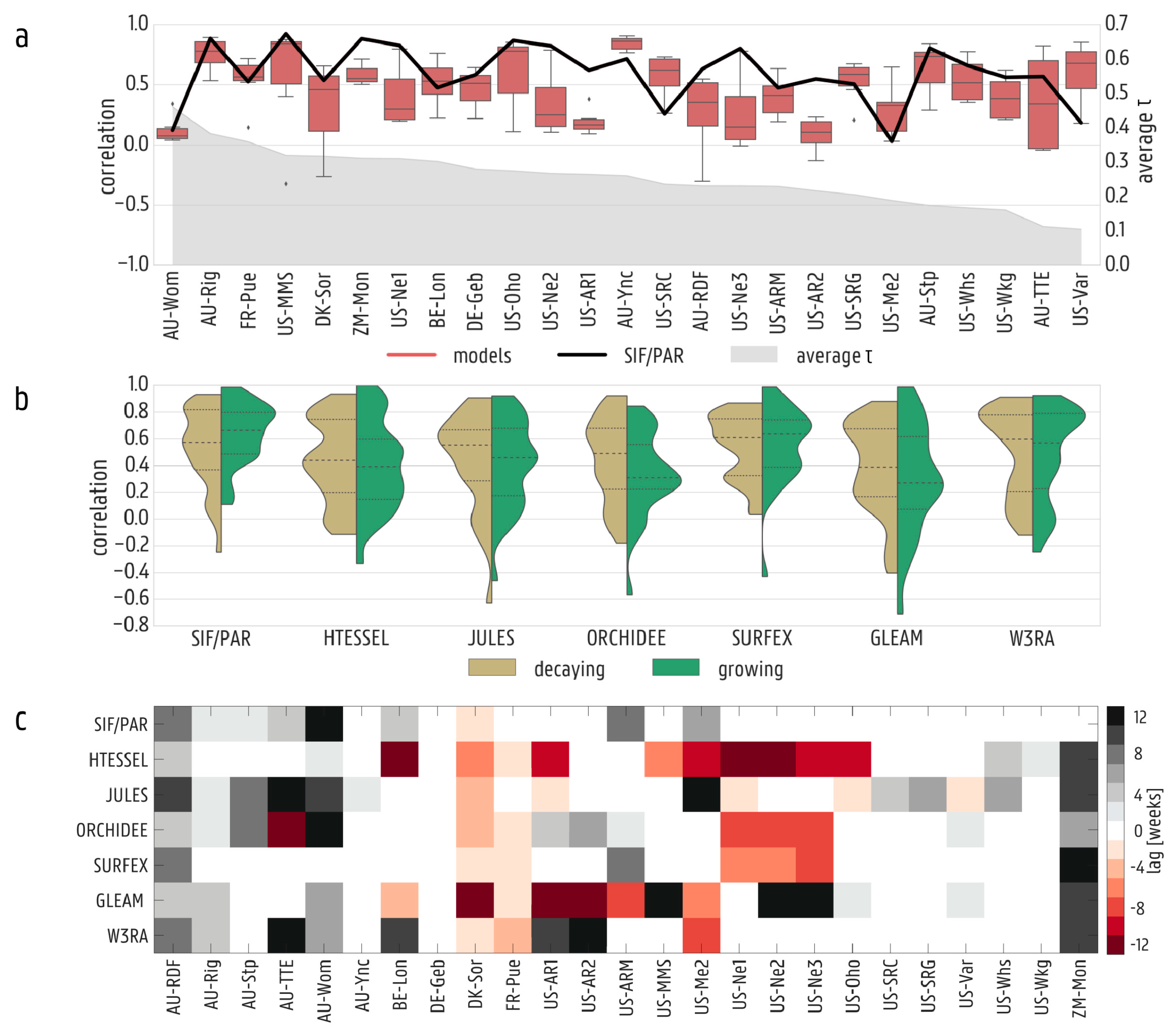
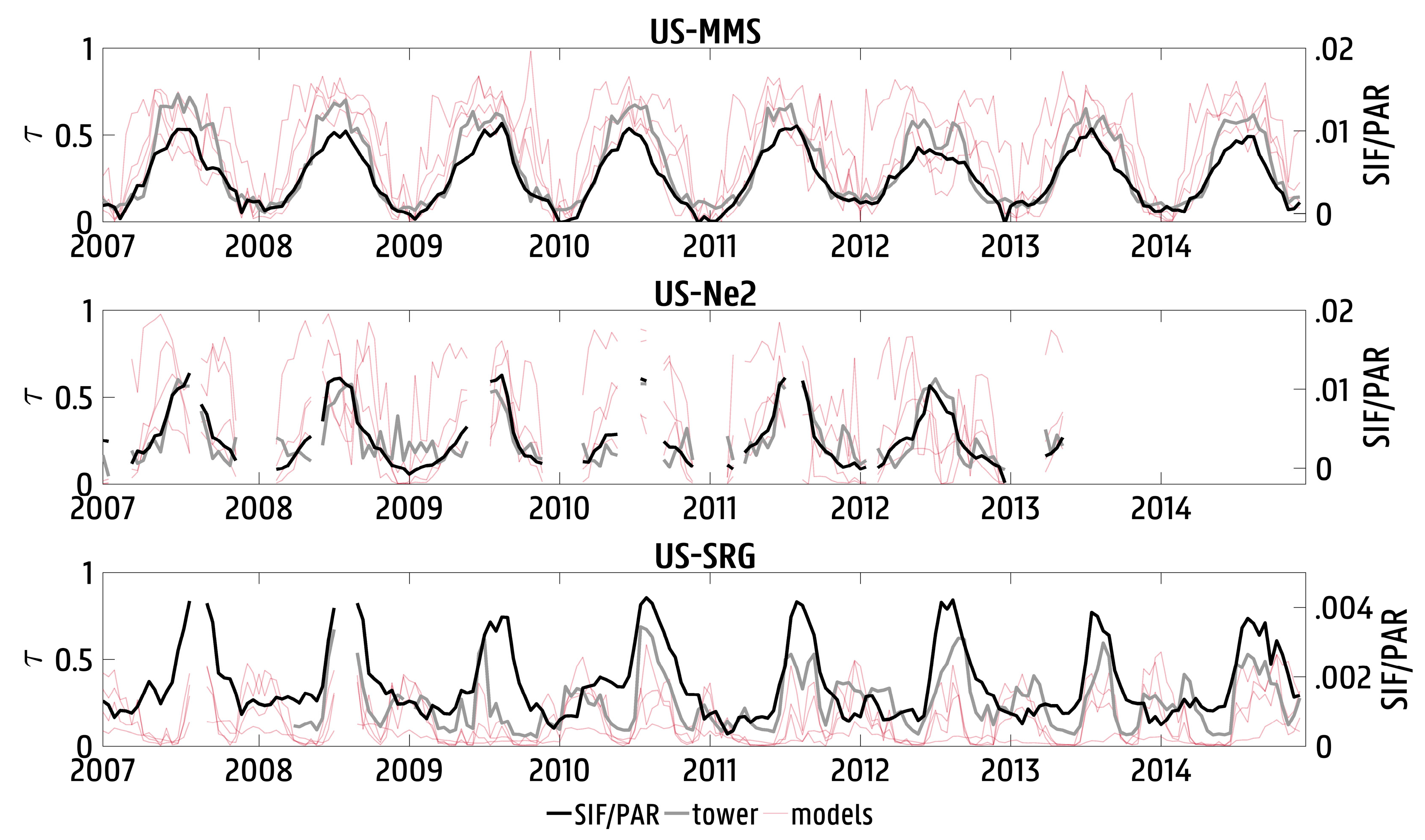
3.1. Validation against In Situ Data

Average Pearson correlation coefficients (R) [80] are calculated based on biweekly aggregates of τ for the period 2007–2014 in comparison to in situ data. Overall, SIF/PAR exhibits an average R = 0.59 for the selection of flux towers, showing individual correlations ranging from R = 0.02 (US-Me2) to R = 0.92 (US-MMS), being statistically significant (p < 0.01) at 22 of the 25 sites. In comparison to individual models, SURFEX (R = 0.56) shows the highest correlations against in situ data; this performance is followed by W3RA (R = 0.50). The remaining models display lower average correlations, ranging from R = 0.09–0.34. The consistently lower performance of some models is further evaluated by analyzing the time series of T and E_p separately against the towers (Figure S2). Results demonstrate that E_p estimates from all models are similar, as expected from their common atmospheric forcing, and that they all compare well to the E_p retrieved at the towers. As such, most of the model-to-tower disagreements in τ result from uncertainties in T: models with higher correlations of T also display a better performance for τ. Figure 2a represents the results of the site validations separately for each individual tower. The overall higher correlations of SIF/PAR against the tower retrievals of τ is evident: for 17 of the 25 sites, correlations are greater than the model ensemble average. Consistently, when correlations are grouped by IGBP biome type at the flux tower scale, the highest correlations between SIF/PAR and the in situ τ data are found at densely forested sites (Figure S3)—some exceptions are further explored in Section 4, including the US-Me2 evergreen needleleaf forest site.

Correlations against in situ data are also explored for months of vegetation growth and decay separately; these periods are defined based on the GPP climatology at each tower. Periods where GPP increases from one month to the next are designated as growing, and those where GPP decreases, designated as decaying. Overall, both SIF/PAR and the models’ τ capture the dynamics at the towers more realistically during the growing season (Figure 2b). Nonetheless, rankings of model performance across both phases are similar to the results over the entire timeframe shown in Figure 2a. SIF/PAR exhibits the highest average R during the growing period (0.64), and compares better to the in situ τ than any of the models. However, during the decaying period, the correlations of SIF/PAR and SURFEX against in situ are comparable (R = 0.53 and R = 0.54, respectively). The remaining models average correlations between 0.30–0.55 during growth and 0.39–0.49 during decay periods.

The ability to capture the timing of transpiration throughout the year is critical for LSMs to be able to simulate the effects of land conditions on temperature, precipitation and radiation adequately [22]. This skill is explored in Figure 2c by computing biweekly cross-correlations against in situ τ retrievals. For SIF/PAR, the maximum cross-correlation against in situ data occurs at zero lag for 16 of the 25 sites. For the remaining sites, SIF/PAR shows a lag in the order of +/– 6 weeks; with the exception of AU-Wom (12 weeks)—results are further discussed in Section 4. Models reflect a wide range of performances, from SURFEX showing maximum cross-correlations at zero lag in a total of 17 of the 25 sites to GLEAM and JULES showing zero lag in only 9 of the 25 sites.

Finally, Figure 3 shows individual time series for three sites (US-MMS, US-Ne2, US-SRG). The three flux towers depicted represent a deciduous broadleaf forest (DBF), cropland (CRO) and grassland (GRA). Time series further demonstrate the ability of SIF/PAR to adequately capture seasonal τ cycles. SIF/PAR most closely follows the tower τ at the DBF site across all seasons compared to the CRO and GRA sites. During the summer months for the CRO site, SIF/PAR does not capture the some of the slight increases in transpiration efficiency (i.e., 2009), which may be due to data resolution (0.5°).

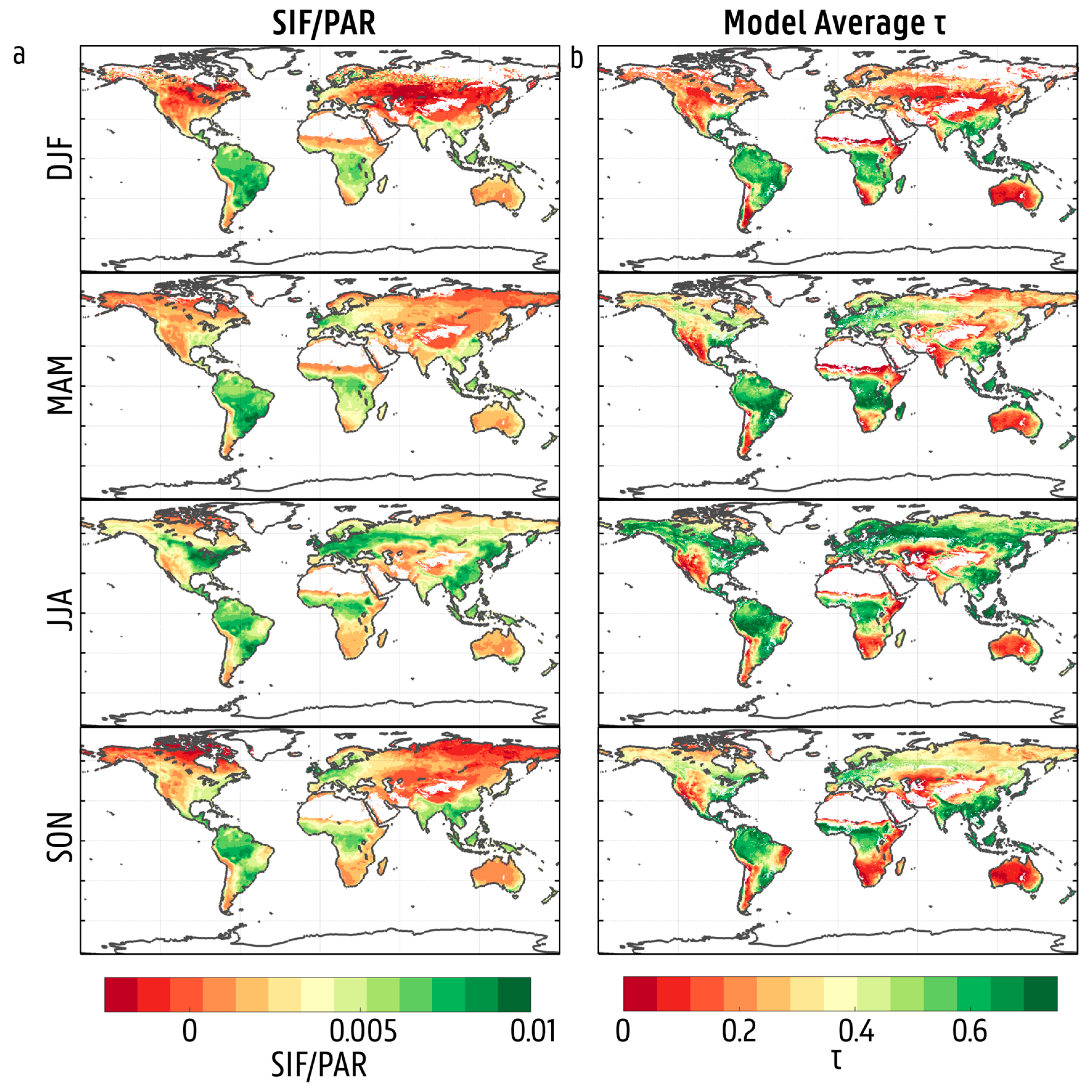
3.2. Spatial and Temporal Variability in Solar-Induced Fluorescence/Photosynthetically Active Radiation (SIF/PAR)

Global seasonal maps of SIF/PAR follow the expected patterns of general vegetation activity in response to different phenological and physiological constraints (Figure 4a). In the Northern Hemisphere, SIF/PAR is lowest during winter (December, January February, (DJF)), suggesting a low transpiration efficiency. In wintertime LAI is lower, with sub-optimal radiation and temperatures, resulting in a reduction of stomatal conductance and carboxylation rates. The highest values (suggesting high transpiration efficiency) occur during the summer (June, July, August (JJA)), when LAI is expected to be high and the vast majority of plant types are active—granted an absence of extreme heat or water stress. In Amazonia, despite the low seasonal variability, SIF/PAR peaks in September, October November (SON). This coincides with the end of the dry season when light availability through the canopy increases, while water is typically not limiting due to the deep rooting structure of emergent species [81,82]. Across the Sahel, SIF/PAR is lowest during DJF and highest during SON, mimicking the timing of the monsoon season. Likewise, in northern Australia, SIF/PAR is the lowest during March, April, May (MAM) and the highest during SON, in phase with the monsoonal rainfall. These spatial and seasonal patterns agree well with the exploration of SIF/PAR by Madani et al. [62]. Finally, Figure 4b displays the seasonal average τ for 2007–2014 for the ensemble of models. While the model ensemble shows markedly lower estimates in water-limited regions, overall spatial patterns agree with those of SIF/PAR, with these similarities being larger for SURFEX and ORCHIDEE—see Figure S4.

4. Discussion

Overall, the results of the validation of SIF/PAR against in situ eddy-covariance estimates reveal the potential of SIF/PAR as a diagnostic of transpiration efficiency. This transpiration efficiency is understood here as the ability of the land cover to meet the atmospheric demand for water, thus may relate to purely phenological variability (e.g., LAI dynamics) as well as to physiological stress related to e.g., extreme climate. SIF/PAR exhibits higher correlations against the in situ data compared to any of the eartH2Observe models, despite its coarser resolution (0.5° versus 0.25°). In a few sites, some models exhibit equivalent or higher performance than SIF/PAR. It is important to note that despite smoothing daily values and using biweekly averages, sensor noise may still be prevalent in SIF/PAR calculations. Nonetheless, the Köhler et al. [47] GOME-2 retrievals tend to exhibit less noise than those from other methods (see ibid.). Future satellites like the European Space Agency’s Fluorescence Explorer (FLEX) or the recently-launched Sentinel 5P (mounting the TROPOMI sensor) are expected to improve these insufficiencies.

When analyzing the validation results grouped by IGBP biome class, SIF/PAR is particularly correlated with the in situ data over densely forested sites, along with grasslands and croplands. SIF/PAR exhibits marked improvements in correlations (0.67) compared to the model average (0.47) for these particular IGBP classes. In contrast, evergreen broadleaf and needleleaf forest sites, like US-Me2, show lower correlations; Madani et al. [62] found similar results when relating SIF with tower GPP (see Figure S3). Further validations indicate that SIF/PAR captures the timing of transpiration efficiency accurately (Figure 2c), and may thus be used to evaluate drought periods. While other optical vegetation indices can be considered, SIF is the only physically-representative remote sensing variable that is expected to capture short-term dynamics in vegetation activity, thus reflect the early stages of transpiration stress. Consequently, SIF has been shown to exhibit the shortest lags with respect to the in situ estimates of latent heat, when compared to traditional optical indices such as LAI, normalized difference vegetation index (NDVI) and enhanced vegetation index (EVI) (see Maes et al. [44,65]).

A potential limitation of our analysis is the lack of validation towers in the Southern Hemisphere, and the fact that not every IGBP class is represented by the 25 towers used for validation. Therefore, the overwhelming majority of towers used in this analysis are clustered in northern mid to high latitudes. Moreover, these sites experience seasonal snow in winter, corresponding to times of declining GPP. Subsequent precipitation and snow masking limits the number of observations, which may explain why the correlations against the in situ observations are slightly lower during the vegetation decay period (Figure 2c). Furthermore, SIF is not corrected for angular anisotropy, which can negatively impact the quality of the observations [83]. Finally, ‘instantaneous’ SIF/PAR retrievals are here compared to daily-average τ from models and towers, as required by the daily resolution of the eartH2Observe data. Consequently, the early overpass timing of GOME-2 (9:30AM), may penalize the SIF/PAR results, as vegetation activity is not expected to be highest in the early morning.

Overall, seasonal analyses and validations demonstrate the potential of SIF/PAR to capture the integrated effect of multiple environmental stress factors on transpiration, such as heat and water stress in dry times and regions or sub-optimal radiation and temperature in wet and cold regions. For instance, at high latitudes, water is not typically a limiting factor, yet sub-optimal temperature and radiation levels may reduce photosynthesis and thus transpiration. This is clearly captured by SIF/PAR (Figure 4a). Especially for deciduous forests, transpiration constraints are not obviously captured by most models, with the exception of SURFEX and ORCHIDEE (see e.g., Figure S4). In the Amazon rainforest, the highest transpiration efficiency occurs at the end of the dry season (SON), which is consistent with the expectations from non-drought years as reported by previous studies [62,84,85]. The relatively lower SIF/PAR values over the Amazon may directly be linked to the higher noise levels in the SIF retrievals over South America due to the South Atlantic magnetic anomaly [86]. Nonetheless, especially in high latitude and tropical biomes, non-climatic drivers can explain a large fraction of the variability in vegetation dynamics [87]; i.e., factors that are poorly represented in models, such as nutrient availability and short-term natural and anthropogenic disturbances (e.g., fires, logging, harvesting, insect epidemics) can be crucial in these environments [88,89,90,91]. The effective assimilation of SIF in global transpiration formulations would directly reflect these dynamics without the need to prescribe species-dependent sensitivities to these stress factors, as in the case of process-based models.

5. Conclusions

We present a novel diagnostic of transpiration efficiency, understood here as the ability of the land surface to meet the atmospheric demand for water vapor. This diagnostic is based on the ratio of SIF over PAR. Validation suggests that SIF satellite observations can potentially be used to constrain transpiration estimates in land surface models. SIF/PAR combines phenological and physiological constraints on the atmospheric demand for water, and adequately reflects the timing of stress. In congruency with the seasonal results, SIF/PAR appears to be capturing more than just water stress and leaf area changes, by demonstrating sensitivity to other factors such as sub-optimal radiation and temperature levels. However, further analysis is needed to determine the capability of SIF/PAR to capture the impact of drought events or heatwaves on transpiration. Estimates of SIF/PAR can be incorporated into transpiration retrieval models (such as GLEAM) or offline land surface models via data assimilation. Finally, our results support the potential of SIF observations to benchmark climate models. This applies not just to the representation of ecosystem carbon exchange, but also to the estimates of surface water and energy fluxes, at a time in which ecosystem stress is still incorporated in climate models via empirical parameterizations.

References

1. Wei, Z.; Yoshimura, K.; Wang, L.; Miralles, D.G.; Jasechko, S.; Lee, X. Revisiting the contribution of transpiration to global terrestrial evapotranspiration. Geophys. Res. Lett. 2017, 44, 2792–2801. [Google Scholar] [CrossRef] [Green Version]
2. Jasechko, S.; Sharp, Z.D.; Gibson, J.J.; Birks, S.J.; Yi, Y.; Fawcett, P.J. Terrestrial water fluxes dominated by transpiration. Nature 2013, 496, 347–350. [Google Scholar] [CrossRef] [PubMed]
3. Collatz, G.J.; Ball, J.T.; Grivet, C.; Berry, J.A. Physiological and environmental regulation of stomatal conductance, photosynthesis and transpiration: a model that includes a laminar boundary layer. Agric. For. Meteorol. 1991, 54, 107–136. [Google Scholar] [CrossRef]
4. Tardieu, F.; Simonneau, T. Variability among species of stomatal control under fluctuating soil water status and evaporative demand: modelling isohydric and anisohydric behaviours. J. Exp. Bot. 1998, 49, 419–432. [Google Scholar] [CrossRef]
5. Medlyn, B.E.; Duursma, R.A.; Eamus, D.; Ellsworth, D.S.; Prentice, I.C.; Barton, C.V.M.; Crous, K.Y.; De Angelis, P.; Freeman, M.; Wingate, L. Reconciling the optimal and empirical approaches to modelling stomatal conductance. Glob. Chang. Biol. 2011, 17, 2134–2144. [Google Scholar] [CrossRef] [Green Version]
6. Lin, Y.S.; Medlyn, B.E.; Duursma, R.A.; Prentice, I.C.; Wang, H.; Baig, S.; Eamus, D.; De Dios, V.R.; Mitchell, P.; Ellsworth, D.S.; et al. Optimal stomatal behaviour around the world. Nat. Clim. Chang. 2015, 5, 459–464. [Google Scholar] [CrossRef] [Green Version]
7. Combe, M.; Vilà-Guerau De Arellano, J.; Ouwersloot, H.G.; Peters, W. Plant water-stress parameterization determines the strength of land–atmosphere coupling. Agric. For. Meteorol. 2016, 217, 61–73. [Google Scholar] [CrossRef]
8. Peñuelas, J.; Rutishauser, T.; Filella, I. Phenology Feedbacks on Climate Change. Science 2009, 324, 887–888. [Google Scholar] [CrossRef] [Green Version]
9. Bonan, G.B. Forests and Climate Change: Forcings, Feedbacks, and the Climate Benefits of Forests. Science 2008, 320, 1444–1449. [Google Scholar] [CrossRef] [Green Version]
10. Schulze, E.; Kelliher, F.M.; Korner, C.; Lloyd, J.; Leuning, R. Relationships among Maximum Stomatal Conductance, Ecosystem Surface Conductance, Carbon Assimilation Rate, and Plant Nitrogen Nutrition: A Global Ecology Scaling Exercise. Annu. Rev. Ecol. Syst. 1994, 25, 629–662. [Google Scholar] [CrossRef]
11. De Kauwe, M.G.; Zhou, S.X.; Medlyn, B.E.; Pitman, A.J.; Wang, Y.P.; Duursma, R.A.; Prentice, I.C. Do land surface models need to include differential plant species responses to drought? Examining model predictions across a latitudinal gradient in Europe. Biogeosciences 2015, 12, 12349–12393. [Google Scholar] [CrossRef]
12. Richardson, A.D.; Anderson, R.S.; Arain, M.A.; Barr, A.G.; Bohrer, G.; Chen, G.; Chen, J.M.; Ciais, P.; Davis, K.J.; Desai, A.R.; et al. Terrestrial biosphere models need better representation of vegetation phenology: Results from the North American Carbon Program Site Synthesis. Glob. Chang. Biol. 2012, 18, 566–584. [Google Scholar] [CrossRef]
13. Fisher, J.B.; Melton, F.; Middleton, E.; Hain, C.; Anderson, M.; Allen, R.; McCabe, M.F.; Hook, S.; Baldocchi, D.; Townsend, P.A.; et al. The future of evapotranspiration: Global requirements for ecosystem functioning, carbon and climate feedbacks, agricultural management, and water resources. Water Resour. Res. 2017, 53, 2618–2626. [Google Scholar] [CrossRef] [Green Version]
14. Novick, K.A.; Miniat, C.F.; Vose, J.M. Drought limitations to leaf-level gas exchange: results from a model linking stomatal optimization and cohesion-tension theory. Plant. Cell Environ. 2016, 39, 583–596. [Google Scholar] [CrossRef] [PubMed]
15. Sperry, J.S.; Wang, Y.; Wolfe, B.T.; Mackay, D.S.; Anderegg, W.R.L.; McDowell, N.G.; Pockman, W.T. Pragmatic hydraulic theory predicts stomatal responses to climatic water deficits. New Phytol. 2016, 212, 577–589. [Google Scholar] [CrossRef] [PubMed]
16. Sperry, J.S.; Venturas, M.D.; Anderegg, W.R.L.; Mencuccini, M.; Mackay, D.S.; Wang, Y.; Love, D.M. Predicting stomatal responses to the environment from the optimization of photosynthetic gain and hydraulic cost. Plant Cell Environ. 2017, 40, 816–830. [Google Scholar] [CrossRef]
17. Xu, X.; Medvigy, D.; Powers, J.S.; Becknell, J.; Guan, K. Hydrological niche separation explains seasonal and inter-annual variations of vegetation dynamics in seasonally dry tropical forests. New Phytol. 2016, 212, 80–95. [Google Scholar] [CrossRef]
18. Jarvis, P.G. The Interpretation of the Variations in Leaf Water Potential and Stomatal Conductance Found in Canopies in the Field. Philos. Trans. R. Soc. B Biol. Sci. 1976, 273, 593–610. [Google Scholar] [CrossRef]
19. Ball, J.T.; Woodrow, I.E.; Berry, J.A. A Model Predicting Stomatal Conductance and its Contribution to the Control of Photosynthesis under Different Environmental Conditions. In Progress in Photosynthesis Research; Springer: Dordrecht, The Netherlands, 1987; pp. 221–224. ISSN1 978-94-017-0521-9. ISSN2 978-94-017-0519-6. [Google Scholar]
20. Oleson, K.W.; Lawrence, D.M.; Bonan, G.B.; Drewniak, B.; Huang, M.; Koven, C.D.; Levis, S.; Li, F.; Riley, J.; Subin, Z.M.; et al. Technical Description of version 4.5 of the Community Land Model (CLM). Available online: http://opensky.ucar.edu/islandora/object/technotes:515 (accessed on 18 October 2017).
21. Verhoef, A.; Egea, G. Modeling plant transpiration under limited soil water: Comparison of different plant and soil hydraulic parameterizations and preliminary implications for their use in land surface models. Agric. For. Meteorol. 2014, 191, 22–32. [Google Scholar] [CrossRef] [Green Version]
22. Miralles, D.G.; Gentine, P.; Seneviratne, S.I.; Teuling, A.J. Land-atmospheric feedbacks during droughts and heatwaves: state of the science and current challenges. Ann. N. Y. Acad. Sci. 2018, 1–17. [Google Scholar] [CrossRef]
23. Calvet, J.C.; Rivalland, V.; Picon-Cochard, C.; Guehl, J.M. Modelling forest transpiration and CO2 fluxes—Response to soil moisture stress. Agric. For. Meteorol. 2004, 124, 143–156. [Google Scholar] [CrossRef]
24. Krinner, G.; Viovy, N.; de Noblet-Ducoudré, N.; Ogée, J.; Polcher, J.; Friedlingstein, P.; Ciais, P.; Sitch, S.; Prentice, I.C. A dynamic global vegetation model for studies of the coupled atmosphere-biosphere system. Global Biogeochem. Cycles 2005, 19, 1–33. [Google Scholar] [CrossRef]
25. Al, R.E.T.; Ronda, R.J.; de Bruin, H.A.R.; Holtslag, A.A.M.; Ronda, R.J.; de Bruin, H.A.R.; Holtslag, A.A.M. Representation of the canopy conductance in modeling the surface energy budget for low vegetation. J. Appl. Meteorol. 2001, 40, 1431–1444. [Google Scholar]
26. Miralles, D.G.; Holmes, T.R.H.; De Jeu, R.A.M.; Gash, J.H.; Meesters, A.G.C.A.; Dolman, A.J. Global land-surface evaporation estimated from satellite-based observations. Hydrol. Earth Syst. Sci. 2011, 15, 453–469. [Google Scholar] [CrossRef] [Green Version]
27. Döll, P.; Fiedler, K.; Zhang, J. Global-scale analysis of river flow alterations due to water withdrawals and reservoirs. Hydrol. Earth Syst. Sci. 2009, 13, 2413–2432. [Google Scholar] [CrossRef] [Green Version]
28. Flörke, M.; Kynast, E.; Bärlund, I.; Eisner, S.; Wimmer, F.; Alcamo, J. Domestic and industrial water uses of the past 60 years as a mirror of socio-economic development: A global simulation study. Glob. Environ. Chang. 2013, 23, 144–156. [Google Scholar] [CrossRef]
29. Gardelin, M.; Lindstrom, G. Priestley-Taylor evapotranspiration in HBV-simulations. Nord. Hydrol. 1997, 28, 233–246. [Google Scholar] [CrossRef]
30. Fisher, J.B.; Baldocchi, D.D.; Misson, L.; Dawson, T.E.; Goldstein, A.H. What the towers don’t see at night: nocturnal sap flow in trees and shrubs at two AmeriFlux sites in California. Tree Physiol. 2007, 27, 597–610. [Google Scholar] [CrossRef]
31. Dhungel, R.; Allen, R.G.; Robison, C.W. Evapotranspiration between satellite overpasses: methodology and case study in agricultural dominant semi-arid areas. Meteorol. Appl. 2016, 730, 714–730. [Google Scholar] [CrossRef]
32. Norman, J.M.; Kustas, W.P.; Humes, K.S. Source approach for estimating soil and vegetation energy fluxes in observations of directional radiometric surface temperature. Agric. For. Meteorol. 1995, 77, 263–293. [Google Scholar] [CrossRef]
33. Colaizzi, P.D.; Kustas, W.P.; Anderson, M.C.; Agam, N.; Tolk, J.A.; Evett, S.R.; Howell, T.A.; Gowda, P.H.; O’Shaughnessy, S.A. Two-source energy balance model estimates of evapotranspiration using component and composite surface temperatures. Adv. Water Resour. 2012, 50, 134–151. [Google Scholar] [CrossRef]
34. Dolman, A.J.; Miralles, D.G.; de Jeu, R.A.M. Fifty years since Monteith’s 1965 seminal paper: The emergence of global ecohydrology. Ecohydrology 2014, 7, 897–902. [Google Scholar] [CrossRef]
35. Miralles, D.G.; Jiménez, C.; Jung, M.; Michel, D.; Ershadi, A.; Mccabe, M.F.; Hirschi, M.; Martens, B.; Dolman, A.J.; Fisher, J.B.; et al. The WACMOS-ET project—Part 2: Evaluation of global terrestrial evaporation data sets. Hydrol. Earth Syst. Sci. 2016, 20, 823–842. [Google Scholar] [CrossRef]
36. McCabe, M.F.; Ershadi, A.; Jimenez, C.; Miralles, D.G.; Michel, D.; Wood, E.F. The GEWEX LandFlux project: Evaluation of model evaporation using tower-based and globally gridded forcing data. Geosci. Model Dev. 2016, 9, 283–305. [Google Scholar] [CrossRef]
37. Jung, M.; Reichstein, M.; Bondeau, A. Towards global empirical upscaling of FLUXNET eddy covariance observations: Validation of a model tree ensemble approach using a biosphere model. Biogeosciences 2009, 6, 2001–2013. [Google Scholar]
38. Talsma, C.J.; Good, S.P.; Jimenez, C.; Martens, B.; Fisher, J.B.; Miralles, D.G.; McCabe, M.F.; Purdy, A.J. Partitioning of evapotranspiration in remote sensing-based models. Agric. For. Meteorol. 2018, 260–261, 131–143. [Google Scholar] [CrossRef]
39. Baker, N.R. Chlorophyll Fluorescence: A Probe of Photosynthesis In Vivo. Annu. Rev. Plant Biol. 2008, 59, 89–113. [Google Scholar] [CrossRef]
40. Papageorgiou, G. Chlorophyll fluorescence: An intrinsic probe of photosynthesis. Bioenerg. Photosynth. 1975, 319–371. [Google Scholar]
41. Porcar-Castell, A.; Tyystjärvi, E.; Atherton, J.; van der Tol, C.; Flexas, J.; Pfündel, E.E.; Moreno, J.; Frankenberg, C.; Berry, J.A. Linking chlorophyll a fluorescence to photosynthesis for remote sensing applications: mechanisms and challenges. J. Exp. Bot. 2014, 65, 4065–4095. [Google Scholar] [CrossRef] [Green Version]
42. Alemohammad, S.H.; Fang, B.; Konings, A.G.; Green, J.K.; Kolassa, J.; Prigent, C.; Aires, F.; Miralles, D.; Gentine, P. Water, Energy, and Carbon with Artificial Neural Networks (WECANN): A statistically-based estimate of global surface turbulent fluxes using solar-induced fluorescence. Biogeosci. Discuss. 2017, 1–36. [Google Scholar] [CrossRef]
43. Cendrero-Mateo, M.P.; Carmo-Silva, A.E.; Porcar-Castell, A.; Hamerlynck, E.P.; Papuga, S.A.; Moran, M.S. Dynamic response of plant chlorophyll fluorescence to light, water and nutrient availability. Funct. Plant Biol. 2015, 42, 746–757. [Google Scholar] [CrossRef]
44. Lu, X.; Liu, Z.; An, S.; Miralles, D.G.; Maes, W.; Liu, Y.; Tang, J. Potential of solar-induced chlorophyll fluorescence to estimate transpiration in a temperate forest. Agric. For. Meteorol. 2018, 252, 75–87. [Google Scholar] [CrossRef]
45. Frankenberg, C.; Fisher, J.B.; Worden, J.; Badgley, G.; Saatchi, S.S.; Lee, J.-E.; Toon, G.C.; Butz, A.; Jung, M.; Kuze, A.; et al. New global observations of the terrestrial carbon cycle from GOSAT: Patterns of plant fluorescence with gross primary productivity. Geophys. Res. Lett. 2011, 38. [Google Scholar] [CrossRef] [Green Version]
46. Joiner, J.; Yoshida, Y.; Vasilkov, A.P.; Corp, L.A.; Middleton, E.M. First observations of global and seasonal terrestrial chlorophyll fluorescence from space. Biogeosciences 2011, 8, 637–651. [Google Scholar] [CrossRef] [Green Version]
47. Köhler, P.; Guanter, L.; Joiner, J. A linear method for the retrieval of sun-induced chlorophyll fluorescence from GOME-2 and SCIAMACHY data. Atmos. Meas. Tech. 2015, 8, 2589–2608. [Google Scholar] [CrossRef] [Green Version]
48. Guanter, L.; Zhang, Y.; Jung, M.; Joiner, J.; Voigt, M.; Berry, J.A.; Frankenberg, C.; Huete, A.R.; Zarco-Tejada, P.; Lee, J.-E.; et al. Global and time-resolved monitoring of crop photosynthesis with chlorophyll fluorescence. Proc. Natl. Acad. Sci. USA 2014, 111, E1327–E1333. [Google Scholar] [CrossRef] [Green Version]
49. Guanter, L.; Frankenberg, C.; Dudhia, A.; Lewis, P.E.; Gómez-Dans, J.; Kuze, A.; Suto, H.; Grainger, R.G. Retrieval and global assessment of terrestrial chlorophyll fluorescence from GOSAT space measurements. Remote Sens. Environ. 2012, 121, 236–251. [Google Scholar] [CrossRef]
50. Köhler, P.; Frankenberg, C.; Magney, T.S.; Guanter, L.; Joiner, J.; Landgraf, J. Global Retrievals of Solar-Induced Chlorophyll Fluorescence With TROPOMI: First Results and Intersensor Comparison to OCO-2. Geophys. Res. Lett. 2018, 45, 10456–10463. [Google Scholar] [CrossRef]
51. Jeong, S.J.; Schimel, D.; Frankenberg, C.; Drewry, D.T.; Fisher, J.B.; Verma, M.; Berry, J.A.; Lee, J.E.; Joiner, J. Application of satellite solar-induced chlorophyll fluorescence to understanding large-scale variations in vegetation phenology and function over northern high latitude forests. Remote Sens. Environ. 2017, 190, 178–187. [Google Scholar] [CrossRef]
52. Joiner, J.; Yoshida, Y.; Vasilkov, A.P.; Schaefer, K.; Jung, M.; Guanter, L.; Zhang, Y.; Garrity, S.; Middleton, E.M.; Huemmrich, K.F.; et al. The seasonal cycle of satellite chlorophyll fluorescence observations and its relationship to vegetation phenology and ecosystem atmosphere carbon exchange. Remote Sens. Environ. 2014, 152, 375–391. [Google Scholar] [CrossRef] [Green Version]
53. Wang, S.; Huang, C.; Zhang, L.; Lin, Y.; Cen, Y.; Wu, T. Monitoring and assessing the 2012 drought in the great plains: Analyzing satellite-retrieved solar-induced chlorophyll fluorescence, drought indices, and gross primary production. Remote Sens. 2016, 8, 61. [Google Scholar] [CrossRef]
54. Shan, N.; Ju, W.; Migliavacca, M.; Martini, D.; Guanter, L.; Chen, J.; Goulas, Y.; Zhang, Y. Modeling canopy conductance and transpiration from solar-induced chlorophyll fluorescence. Agric. For. Meteorol. 2019, 268, 189–201. [Google Scholar] [CrossRef]
55. Lee, J.-E.; Berry, J.A.; van der Tol, C.; Yang, X.; Guanter, L.; Damm, A.; Baker, I.; Frankenberg, C. Simulations of chlorophyll fluorescence incorporated into the Community Land Model version 4. Glob. Chang. Biol. 2015, 21, 3469–3477. [Google Scholar] [CrossRef] [PubMed] [Green Version]
56. Norton, A.J.; Rayner, P.J.; Koffi, E.N.; Scholze, M. Assimilating solar-induced chlorophyll fluorescence into the terrestrial biosphere model BETHY-SCOPE: Model description and information content. Geosci. Model Dev. Discuss. 2018, 11, 1–26. [Google Scholar] [CrossRef]
57. Schellekens, J.; Dutra, E.; Martínez-de la Torre, A.; Balsamo, G.; van Dijk, A.; Weiland, F.S.; Minvielle, M.; Calvet, J.-C.; Decharme, B.; Eisner, S. A global water resources ensemble of hydrological models: The eartH2Observe Tier-1 dataset. Earth Syst. Sci. Data 2017, 9, 389. [Google Scholar] [CrossRef]
58. Sun, Y.; Frankenberg, C.; Wood, J.D.; Schimel, D.S.; Jung, M.; Guanter, L.; Drewry, D.T.; Verma, M.; Porcar-Castell, A.; Griffis, T.J.; et al. OCO-2 advances photosynthesis observation from space via solar-induced chlorophyll fluorescence. Science 2017, 358. [Google Scholar] [CrossRef] [PubMed]
59. Wieneke, S.; Ahrends, H.; Damm, A.; Pinto, F.; Stadler, A.; Rossini, M.; Rascher, U. Airborne based spectroscopy of red and far-red sun-induced chlorophyll fluorescence: Implications for improved estimates of gross primary productivity. Remote Sens. Environ. 2016, 184, 654–667. [Google Scholar] [CrossRef] [Green Version]
60. Rigden, A.J.; Salvucci, G.D.; Entekhabi, D.; Short Gianotti, D.J. Partitioning Evapotranspiration Over the Continental United States Using Weather Station Data. Geophys. Res. Lett. 2018, 45, 9605–9613. [Google Scholar] [CrossRef]
61. Zhou, S.; Yu, B.; Zhang, Y.; Huang, Y.; Wang, G. Partitioning evapotranspiration based on the concept of underlying water use efficiency. Water Resour. Res. 2016, 52, 1160–1175. [Google Scholar] [CrossRef]
62. Madani, N.; Kimball, J.; Jones, L.; Parazoo, N.; Guan, K. Global Analysis of Bioclimatic Controls on Ecosystem Productivity Using Satellite Observations of Solar-Induced Chlorophyll Fluorescence. Remote Sens. 2017, 9, 530. [Google Scholar] [CrossRef]
63. Maes, W.H.H.; Gentine, P.; Verhoest, N.E.C.E.C.; Miralles, D.G.G. Potential evaporation at eddy-covariance sites across the globe. Hydrol. Earth Syst. Sci. Discuss. 2019, 1–33. [Google Scholar]
64. Milly, P.C.D.; Dunne, K.A. Potential evapotranspiration and continental drying. Nat. Clim. Chang. 2016, 6, 946–949. [Google Scholar] [CrossRef]
65. Maes, W.; Gentine, P.; Steppe, K.; Verhoest, N.E.C.; Dorigo, W.A.; Miralles, D.G. Solar-induced fluorescence: The best alternative to monitor global transpiration? In Proceedings of the EGU, Vienna, Austria, 4–13 April 2018. [Google Scholar]
66. Wielicki, B.A.; Barkstrom, B.R.; Harrison, E.F.; Lee, R.B.; Smith, G.L.; Cooper, J.E. Clouds and the Earth’s Radiant Energy System (CERES): An Earth Observing System Experiment. Bull. Am. Meteorol. Soc. 1996, 77, 853–868. [Google Scholar] [CrossRef]
67. Luojus, K.; Pulliainen, J.; Takala, M.; Lemmetyinen, J.; Kangwa, M.; Smolander, T.; Derksen, C. Global Snow Monitoring for Climate Research: Algorithm Theoretical Basis Document (ATBD)–SWE-Algorithm. In Technical Report. 2013. Available online: http://www.globsnow.info/docs/GS2_SWE_ATBD.pdf (accessed on 29 September 2017).
68. Tucker, C.J.; Pinzon, J.E.; Brown, M.E.; Slayback, D.A.; Pak, E.W.; Mahoney, R.; Vermote, E.F.; El Saleous, N. An extended AVHRR 8-km NDVI dataset compatible with MODIS and SPOT vegetation NDVI data. Int. J. Remote Sens. 2005, 26, 4485–4498. [Google Scholar] [CrossRef]
69. Pizon, J.; Brown, M.; Tucker, C. Satellite time series correction of orbital drift artifacts using empirical mode decomposition. Hilbert-Huang Transform Introd. Appl. 2005, 167–186. [Google Scholar]
70. Beck, H.E.; Van Dijk, A.I.J.M.; Levizzani, V.; Schellekens, J.; Miralles, D.G.; Martens, B.; De Roo, A. MSWEP: 3-hourly 0.25° global gridded precipitation (1979–2015) by merging gauge, satellite, and reanalysis data. Hydrol. Earth Syst. Sci. 2017, 21, 589–615. [Google Scholar] [CrossRef] [Green Version]
71. Martens, B.; Miralles, D.G.; Lievens, H.; van der Schalie, R.; de Jeu, R.A.M.; Férnandez-Prieto, D.; Beck, H.E.; Dorigo, W.A.; Verhoest, N.E.C. GLEAM v3: Satellite-based land evaporation and root-zone soil moisture. Geosci. Model Dev. Discuss. 2017, 1–36. [Google Scholar] [CrossRef]
72. van Dijk, A.I.J.M.; Renzullo, L.J.; Wada, Y.; Tregoning, P. A global water cycle reanalysis (2003-2012) merging satellite gravimetry and altimetry observations with a hydrological multi-model ensemble. Hydrol. Earth Syst. Sci. 2014, 18, 2955–2973. [Google Scholar] [CrossRef]
73. Van Dijk, A.; Warren, G. The Australian Water Resources Assessment System. Technical Report 4. Landscape Model (version 0.5) Evaluation Against Observations. CSIRO: Water for a Healthy Country National Research Flagship. 2010. Available online: http://www.clw.csiro.au/publications/waterforahealthycountry/2010/wfhc-awras-evaluation-against-observations.pdf (accessed on 24 October 2017).
74. Balsamo, G.; Beljaars, A.; Scipal, K.; Viterbo, P.; van den Hurk, B.; Hirschi, M.; Betts, A.K. A revised hydrology for the ECMWF model: Verification from field site to terrestrial water storage and impact in the Integrated Forecast System. J. Hydrometeorol. 2009, 10, 623–643. [Google Scholar] [CrossRef]
75. Yamazaki, D.; Kanae, S.; Kim, H.; Oki, T. A physically based description of floodplain inundation dynamics in a global river routing model. Water Resour. Res. 2011, 47, 1–21. [Google Scholar] [CrossRef]
76. Clark, D.B.; Mercado, L.M.; Sitch, S.; Jones, C.D.; Gedney, N.; Best, M.J.; Pryor, M.; Rooney, G.G.; Essery, R.L.H.; Blyth, E.; et al. The Joint UK Land Environment Simulator (JULES), Model description—Part 2: Carbon fluxes and vegetation. Geosci. Model Dev. Discuss. 2011, 4, 641–688. [Google Scholar] [CrossRef]
77. d’Orgeval, T.; Polcher, J.; de Rosnay, P. Sensitivity of the West African hydrological cycle in ORCHIDEE to infiltration processes. Hydrol. Earth Syst. Sci. 2008, 12, 1387–1401. [Google Scholar] [CrossRef] [Green Version]
78. Decharme, B.; Alkama, R.; Douville, H.; Becker, M.; Cazenave, A. Global Evaluation of the ISBA-TRIP Continental Hydrological System. Part II: Uncertainties in River Routing Simulation Related to Flow Velocity and Groundwater Storage. J. Hydrometeorol. 2010, 11, 601–617. [Google Scholar] [CrossRef] [Green Version]
79. Decharme, B.; Martin, E.; Faroux, S. Reconciling soil thermal and hydrological lower boundary conditions in land surface models. J. Geophys. Res. Atmos. 2013, 118, 7819–7834. [Google Scholar] [CrossRef] [Green Version]
80. Pearson, K. Note on Regression and Inheritance in the Case of Two Parents. Proc. R. Soc. London 1895. [Google Scholar]
81. Huete, A.R.; Didan, K.; Shimabukuro, Y.E.; Ratana, P.; Saleska, S.R.; Hutyra, L.R.; Yang, W.; Nemani, R.R.; Myneni, R. Amazon rainforests green-up with sunlight in dry season. Geophys. Res. Lett. 2006, 33, 2–5. [Google Scholar] [CrossRef]
82. Lopes, A.P.; Nelson, B.W.; Wu, J.; de Alencastro Graça, P.M.; Tavares, J.V.; Prohaska, N.; Martins, G.A.; Saleska, S.R. Leaf flush drives dry season green-up of the Central Amazon. Remote Sens. Environ. 2016, 182, 90–98. [Google Scholar] [CrossRef]
83. He, L.; Chen, J.M.; Liu, J.; Mo, G.; Joiner, J. Angular normalization of GOME-2 Sun-induced chlorophyll fluorescence observation as a better proxy of vegetation productivity. Geophys. Res. Lett. 2017, 44, 5691–5699. [Google Scholar] [CrossRef]
84. Bi, J.; Knyazikhin, Y.; Choi, S.; Park, T.; Barichivich, J.; Ciais, P.; Fu, R.; Ganguly, S.; Hall, F.; Hilker, T.; et al. Sunlight mediated seasonality in canopy structure and photosynthetic activity of Amazonian rainforests. Environ. Res. Lett. 2015, 10, 1–6. [Google Scholar] [CrossRef]
85. Saleska, S.R.; Wu, J.; Guan, K.; Araujo, A.C.; Huete, A.; Nobre, A.D.; Restrepo-Coupe, N. Dry-season greening of Amazon forests. Nature 2016, 531, E4–E5. [Google Scholar] [CrossRef] [PubMed]
86. Köhler, P.; Guanter, L.; Kobayashi, H.; Walther, S.; Yang, W. Assessing the potential of sun-induced fluorescence and the canopy scattering coefficient to track large-scale vegetation dynamics in Amazon forests. Remote Sens. Environ. 2017, 204, 769–785. [Google Scholar] [CrossRef]
87. Papagiannopoulou, C.; Miralles, D.G.; Dorigo, W.A.; Verhoest, N.E.C.; Depoorter, M.; Waegeman, W. Vegetation anomalies caused by antecedent precipitation in most of the world. Environ. Res. Lett. 2017, 12, 074016. [Google Scholar] [CrossRef] [Green Version]
88. Fisher, J.B.; Badgley, G.; Blyth, E. Global nutrient limitation in terrestrial vegetation. Global Biogeochem. Cycles 2012, 26, 1–9. [Google Scholar] [CrossRef]
89. Reichstein, M.; Bahn, M.; Ciais, P.; Frank, D.; Mahecha, M.D.; Seneviratne, S.I.; Zscheischler, J.; Beer, C.; Buchmann, N.; Frank, D.C.; et al. Climate extremes and the carbon cycle. Nature 2013, 500, 287–295. [Google Scholar] [CrossRef] [PubMed]
90. Le Quéré, C.; Andrew, R.M.; Canadell, J.G.; Sitch, S.; Korsbakken, J.I.; Peters, G.P.; Manning, A.C.; Boden, T.A.; Tans, P.P.; Houghton, R.A.; et al. Global Carbon Budget 2016. Earth Syst. Sci. Data 2016, 8, 605–649. [Google Scholar] [CrossRef] [Green Version]
91. Zhu, Z.; Piao, S.; Myneni, R.B.; Huang, M.; Zeng, Z.; Canadell, J.G.; Ciais, P.; Sitch, S.; Friedlingstein, P.; Arneth, A.; et al. Greening of the Earth and its drivers. Nat. Clim. Chang. 2016, 6, 791–795. [Google Scholar] [CrossRef] [Green Version]
Figure 1. The hypothesis. Conceptual diagram of the expected surface energy balance and photosynthetically active radiation (PAR) partitioning in response to phenological and physiological constraints. Variables represent the absorbed PAR (i.e., aPAR), solar-induced fluorescence (SIF), non-radiative decay and non-photochemical quenching (Q), gross primary production (GPP), net radiation (Rn), latent heat (λE), sensible heat (H) and ground heat flux (G).
Remotesensing 11 00413 g001
Figure 2. In situ validation. (a) Correlations of flux tower sites versus eartH2Observe models (red boxplots) and SIF/PAR (black line) ordered by fraction of bare soil (grey shade, top). (b) Results during decaying (gold) and growing (green) periods separately (as defined by average monthly climatologies of tower GPP) for SIF/PAR and each model across flux tower sites. (c) Lag at which the cross-correlations for each model and SIF/PAR versus the FLUXNET towers are maximum. Negative values imply an early onset of phenological and/or physiological constraints, while positive implies a delay relative to towers.
Remotesensing 11 00413 g002
Figure 3. Timing of transpiration efficiency (τ). Bi-weekly times series of τ from the flux tower sites US-MMS (deciduous broadleaf forest), US-Ne2 (crop) and US-SRG (grassland) compared to SIF/PAR and the eartH2Observe models for 2007–2014. Precipitation and snow dates are masked.
Remotesensing 11 00413 g003
Figure 4. SIF/PAR (a) and model ensemble τ (b) are averaged across each season (December, January February (DJF); March, April, May (MAM); June, July, August (JJA); and September, October November (SON)) between 2007–2014. Higher values of both SIF/PAR and τ (green regions) indicate unstressed conditions and dense vegetation, while lower values (red regions) indicate greater transpiration constraints. Pixels designated as barren or snow and ice based on the International Geosphere-Biosphere Programme (IGBP) classification are masked out. Pixels with less than 30 days of observations per season are also excluded.
Remotesensing 11 00413 g004