A Comparison of Hybrid Machine Learning Algorithms for the Retrieval of Wheat Biophysical Variables from Sentinel-2

Abstract

This study focuses on the comparison of hybrid methods of estimation of biophysical variables such as leaf area index (LAI), leaf chlorophyll content (LCC), fraction of absorbed photosynthetically active radiation (FAPAR), fraction of vegetation cover (FVC), and canopy chlorophyll content (CCC) from Sentinel-2 satellite data. Different machine learning algorithms were trained with simulated spectra generated by the physically-based radiative transfer model PROSAIL and subsequently applied to Sentinel-2 reflectance spectra. The algorithms were assessed against a standard operational approach, i.e., the European Space Agency (ESA) Sentinel Application Platform (SNAP) toolbox, based on neural networks. Since kernel-based algorithms have a heavy computational cost when trained with large datasets, an active learning (AL) strategy was explored to try to alleviate this issue. Validation was carried out using ground data from two study sites: one in Shunyi (China) and the other in Maccarese (Italy). In general, the performance of the algorithms was consistent for the two study sites, though a different level of accuracy was found between the two sites, possibly due to slightly different ground sampling protocols and the range and variability of the values of the biophysical variables in the two ground datasets. For LAI estimation, the best ground validation results were obtained for both sites using least squares linear regression (LSLR) and partial least squares regression, with the best performances values of R² of 0.78, rott mean squared error (RMSE) of 0.68 m² m⁻² and a relative RMSE (RRMSE) of 19.48% obtained in the Maccarese site with LSLR. The best results for LCC were obtained using Random Forest Tree Bagger (RFTB) and Bagging Trees (BagT) with the best performances obtained in Maccarese using RFTB (R² = 0.26, RMSE = 8.88 μg cm⁻², RRMSE = 17.43%). Gaussian Process Regression (GPR) was the best algorithm for all variables only in the cross-validation phase, but not in the ground validation, where it ranked as the best only for FVC in Maccarese (R² = 0.90, RMSE = 0.08, RRMSE = 9.86%). It was found that the AL strategy was more efficient than the random selection of samples for training the GPR algorithm.

1. Introduction

Accurate quantitative estimation of biophysical variables is of crucial importance for different agricultural and ecological applications. Such variables include leaf area index (LAI), leaf chlorophyll content (LCC), fraction of absorbed photosynthetically active radiation (FAPAR), fractional vegetation cover (FVC), and canopy chlorophyll content (CCC). Their knowledge is valuable, for example, for precision agriculture [1], crop traits monitoring [2], and improved yield prediction and reduction of fertilizer usage [3,4]. The retrieval of vegetation biophysical variables from multispectral optical satellite data has been performed by many studies in the last decades [2,5]. In time, there have been significant developments in the algorithms used for such tasks, with a shift from empirical to more physically-based approaches. Starting from simple parametric regressions between vegetation indices and biophysical variables such as LAI and LCC [6,7,8], the current state of the art relies on hybrid methods exploiting at the same time radiative transfer models (RTM) and non-linear non-parametric regression algorithms [5,9,10]. The methods based on the relationship of, for example, vegetation indices and biophysical variables by the means of fitting functions, typically use the information provided by two or a few spectral bands. This limits the strength of such methods in today’s scenarios where tens or even hundreds of spectral bands are available, respectively, in current super-spectral [11] or forthcoming hyperspectral [12,13] spaceborne sensors.

On the other hand, many of the approaches that have been more recently developed for the retrieval of biophysical variables exploit machine learning regression algorithms (MLRAs). These algorithms have gained wide popularity since they allow the use of more complex models, by requiring only one time-consuming training phase, but allowing their fast application any time thereafter for the retrieval [14,15]. Another advantage of these algorithms is the possibility of training them with full spectral information, thus overcoming issues of band selection or transformation, as in the case of parametric regression methods [16]. These algorithms are adaptive and have the ability to cope with the strong non-linearity inherent in remote sensing data [17,18]. Despite their advantages, these algorithms are computationally demanding, so for some MLRAs it is difficult to carry out a training phase with a large number of samples, though there are some that perform well also when trained with small datasets [19]. Some of the MLRAs are also considered black boxes, e.g., neural networks (NNs) [11,20], in which no insight is given about the physical processes linking the spectral reflectance with the biophysical variables. Others, such as partial least squares regression (PLSR) or Gaussian processes regression (GPR), can instead provide some information on what spectral bands are more relevant. In hybrid methods, MLRA can be trained using physically-based modelling approaches that describe the transfer and interaction of radiation inside the canopy based on physical laws, thus providing explicit relations between the biophysical variables and canopy spectral reflectance. When used in the direct mode, biophysical variables are used as input to the physical based RTM, which in turn simulates the top-of-canopy (TOC) spectral reflectance [9]. Using turbid-medium RTMs it is easy to generate during a short time a large simulated database, with realistic ranges of variation of biophysical variables and their corresponding simulated spectra, within the limits of the assumptions of the RTM on canopy properties. These pairs of biophysical variables and reflectance spectra can be used either in numerical optimization or in look up table (LUT) retrieval methods, by minimizing a cost function expressing the differences between observed (e.g., from satellite data) and RTM model’s simulated reflectance and looking up the corresponding values of the biophysical variables [21]. For operational applications, due to the pixel-by-pixel calculations, these algorithms are computationally very demanding. These methods are also strongly affected by noise and measurement uncertainties [11]. As inversion methods of physically-based RTMs, they suffer from the limitation of the ill-posed nature of model inversion [22,23], by which different combinations of canopy variables lead to local minima having similar reflectance spectra [24].

In the hybrid methods of retrieval, the database obtained from RTM simulations can be used to train MLRA which are able to establish complex non-linear, non-parametric models linking the biophysical variables and the spectral reflectance [9,11]. Hybrid methods have found widespread application and have reached the operational stage, in particular with the application of NNs [25,26,27] trained with the RTM PROSAIL [28,29], such as the algorithm implemented in Sentinel Application Platform (SNAP) biophysical processor tool [29], developed by the European Space Agency (ESA). Leaf area index retrieval using NNs trained with PROSAIL is also carried out operationally for Cyclopes and Moderate Resolution Imaging Spectrometer (MODIS) products [30]. However, NN training is a delicate phase and requires the tuning of multiple parameters, which greatly impacts the robustness of the approach [18]. Thus, in recent years, increasing attention has been paid to alternatives to NNs that are simpler to train and have better potential for retrieval accuracy, such as kernel-based methods [31]. These methods solve non-linear regression problems by transferring the data to a higher dimensional space by the means of a kernel function [16]. Kernel-based algorithms have been suggested to offer some advantages in comparison to NNs. Kernel ridge regression (KRR) has proven to be simple for training and to yield competitive accuracy [18]. Gaussian process regression (GPR) is partially transparent compared to the black box nature of NNs. It allows the use of different kernel functions, ranging from simple to very complex, and it also provides uncertainty estimates with the mean value of prediction [10,32]. Gaussian process regression and KRR have been used to estimate successfully LAI and LCC [10,33]. Unfortunately, some kernel-based algorithms, such as GPR and KRR, are computationally very expensive if trained on large sets of simulations [9,10]. In order to have a general-purpose database, including a wide range of vegetation types, generally a huge number of simulations are performed [10]. However, not all pairs of the reflectance and corresponding biophysical variables will be relevant. Few attempts have been made by the researchers to optimize the simulations that are generated by the physically-based models [10,34]. Active learning (AL) has been proposed as a useful strategy to reduce the size of the RTM-generated database, to make the training of the kernel-based algorithms such as GPR more feasible [10]. Active learning is a sub-field of machine learning, also called optimal experimental design in statistics [35]. It initially starts with a small subset of the samples, and then, based on query strategies using either uncertainty or diversity measurement criteria, adds iteratively new samples to the initial training set of samples. In this way, the most informative samples in a dataset are selected, avoiding redundancy [10]. Active learning techniques have a great potential to optimally sample sets generated by RTM.

Very few studies [9,10] have reported the potential of kernel-based methods using AL techniques in relation to the retrieval of biophysical variables such as LAI, LCC, FVC, FAPAR, and CCC. In particular, although the estimation of these variables from hyperspectral data has been demonstrated [28], the suitability of multispectral satellites has yet to be fully proven, especially for biochemical variables such as LCC. The European Space Agency Sentinel-2 mission has been shown to provide data of a high radiometric quality [36] and has a higher revisit frequency than what is planned for hyperspectral satellites in the near future. Because of the availability of a larger number of spectral bands than other multispectral satellites, and of the inclusion of the red edge region of the spectrum, Sentinel-2 has a good potential for the estimation of these variables [9].

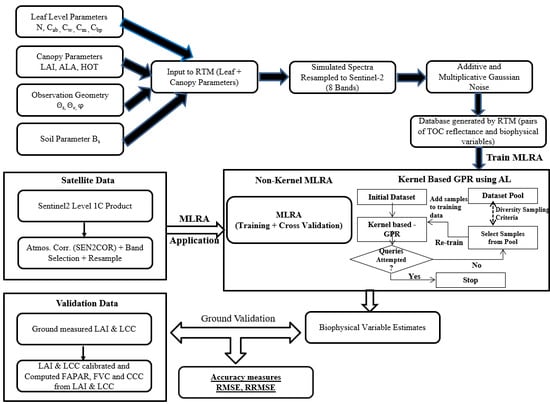
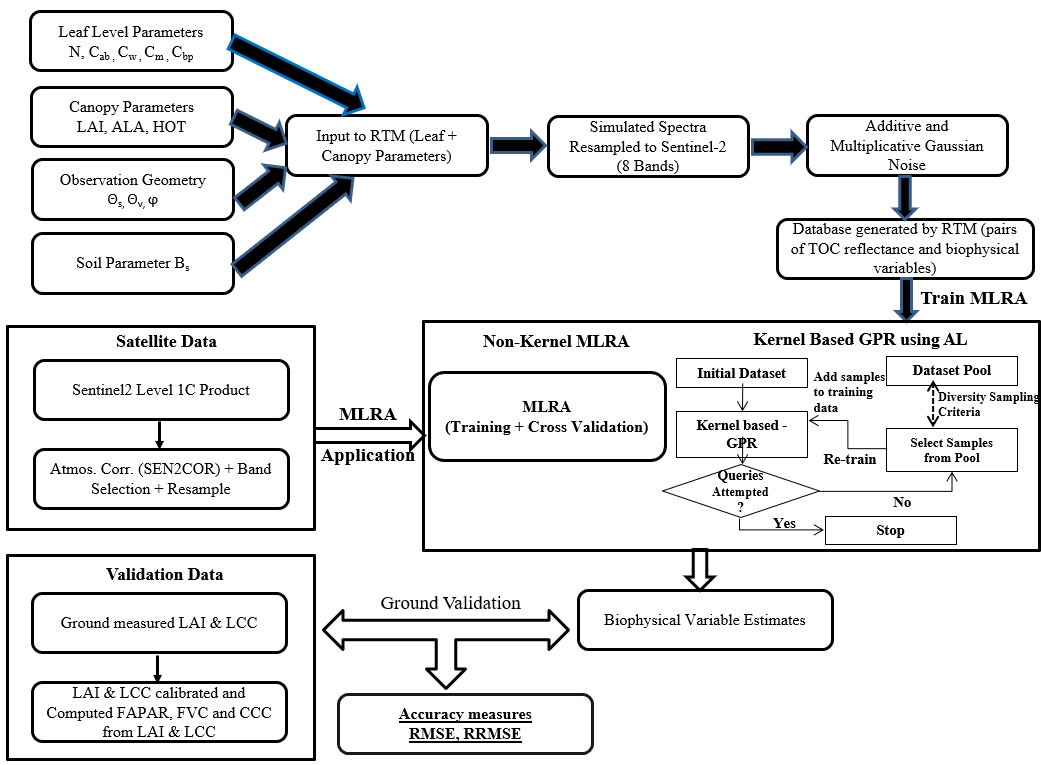
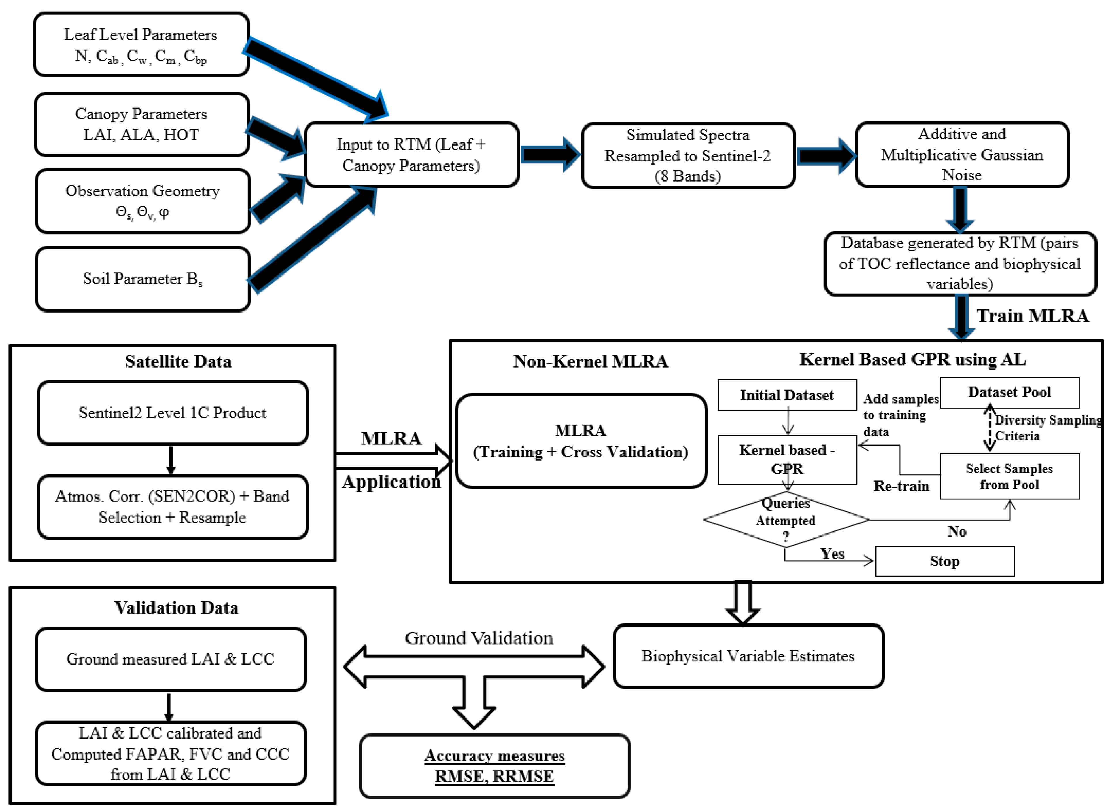
This work explores the application of kernel-based GPR using AL for biophysical variables retrieval from Sentinel-2, comparing the potential of this algorithm with other MLRAs and in particular of the version implemented operationally in SNAP.

The main objectives of this study are thus: (1) to compare the performances of different MLRAs, in particular with respect to the algorithm based on NNs implemented in the biophysical processor tool of the ESA SNAP toolbox, by using the same database of PROSAIL simulations [29]; (2) to assess the accuracy of estimation of the biophysical variables LAI, LCC, FAPAR, CCC, and FVC in the wheat crop, for kernel-based (GPR) and non-kernel-based MLRA hybrid methods of retrieval; (3) to explore the feasibility and potential of the use of AL strategies to optimally sample redundant PROSAIL simulations, to minimize computational time and complexity and allow the use of computationally demanding MLRAs (such as GPR) in hybrid methods.

2. Materials and Methods

The methodology adopted in this work (Figure 1), for the comparison of hybrid methods of biophysical variables retrieval, employed simulations carried out with the model PROSAIL [37] for training MLRA and finally applying them to Sentinel-2 data for assessment with ground measurements collected in two study areas, respectively in Italy and China. The procedure involved the following steps, illustrated in detail in the following sections: (1) generation of simulations with the model PROSAIL; (2) training MLRAs with model simulations and cross-validation; (3) Sentinel-2 data pre-processing; and (4) validation using ground data.

2.1. Generation of PROSAIL Simulations

The model PROSAIL [37] is a widely used RTM for generating realizations of TOC canopy reflectances by considering measured biophysical variables of the crop of interest. It is a combination of the leaf level model PROSPECT [38] and canopy level model SAIL [39]. It has been inverted over a large range of vegetation canopies [40,41,42,43,44,45,46] with varying degrees of success. Reflectance and transmittance of a leaf from the PROSPECT model was used as an input for the SAIL model with the soil optical properties and illumination and observation geometry.

The benchmark against which the different hybrid methods were assessed in this study was the NN algorithm implemented in the ESA SNAP Sentinel-2 Toolbox, as biophysical processor. For this reason, PROSAIL simulations were generated using the same input parameter values and configuration as used for SNAP (M.Weiss personal communication), by following the Sentinel-2 Toolbox level 2 products Algorithm Theoretical Basis Document (ATBD) [29], with the exception of the geometry of observation and illumination which was set only for the conditions of our validation dataset (Section 2.3). The PROSAIL parameters were sampled using a fully orthogonal experimental plan [47], using a component of the BV-NNET (Biophysical Variables Neural Network) tool developed by Reference [48]. This procedure consists of identifying classes of values for each variable. Then all the combinations of classes are sampled once. Finally, the actual values of each variable are randomly drawn within the range of variation defined by the corresponding class, according to the distribution law specified for the variable considered. This process allows to take into account all the interactions among parameters, while having the range of variation for each variable densely and near randomly populated [29].

Table 1. Input parameter value ranges, number of classes, and statistical distributions used for generating the training database with the PROSAIL model.

	Variable	Units	Min	Max	Mode	SD	Class	Law
Canopy	Leaf area index (LAI)	-	0	15	2	2	6	log_normal
	Avearge leaf angle (ALA)	-	30	80	60	20	3	gaussian
	Hot spot parameter (HsD)	-	0.1	0.5	0.2	0.5	1	gaussian
	Leaf structure index (N)	-	1.2	1.8	1.5	0.3	3	gaussian
Leaf	Leaf chlorophyll content (LCC)	µg cm−2	20	90	45	30	4	gaussian
	Leaf dry matter content (Cdm)	g cm−2	0.003	0.011	0.005	0.005	4	gaussian
	Leaf water content (Cw_Rel)	-	0.6	0.85	0.75	0.08	4	uniform
	Brown pigments (Cbp)	-	0	2	0	0.3	3	gaussian
Soil	Soil brightness (Bs)	-	0.5	3.5	1.2	2	4	gaussian

reports the parameter ranges, statistical distribution, and number of classes of the PROSAIL model that were used in the present work, which were the same as those employed for training NNs in SNAP (M. Weiss personal communication). A total of 41,472 simulations were generated, representing an extensive range of vegetation properties.

The PROSAIL model top of the canopy (TOC) full spectra (at 1 nm resolution) were then resampled, using Sentinel-2 spectral response functions, to the same eight bands as used in the Sentinel-2 level 2 products ATBD [29], i.e., bands 3 to 7, 8a, 11, and 12, excluding the bands most affected by atmospheric attenuation. The spectral resampling was carried out according to Equation (1):

$$\mathsf{\rho }=\sum _{\mathrm{i}}^{\mathrm{N}}\left[\frac{\mathsf{\beta }\left(\mathsf{\lambda }\right)}{{\sum }_{\mathrm{i}}^{\mathrm{N}}\mathsf{\beta }\left(\mathsf{\lambda }\right)}\right]\ast \mathsf{\rho }\left(\mathsf{\lambda }\right)$$

(1)

where ρ and ρ(λ) are, respectively, the resampled Sentinel-2 reflectance and the PROSAIL reflectance at wavelength λ. β(λ) represents the weight of the band’s spectral response function of the Sentinel-2 MSI sensor, whereas i and N are, respectively, the minimum and maximum wavelengths of the Sentinel-2 band. Similarly, a Gaussian noise model was used to better describe actual Sentinel-2 characteristics as well as the ability of the RTM used to represent actual reflectance. The noise was computed as follows [29]:

$${\mathrm{R}}^{*}\left(\mathsf{\lambda }\right)=\mathrm{R}\left(\mathsf{\lambda }\right)\left(1+\mathrm{M}\mathrm{D}\left(\mathsf{\lambda }\right)+\mathrm{M}\mathrm{I}\right)/100)+\mathrm{A}\mathrm{D}\left(\mathsf{\lambda }\right)+\mathrm{A}\mathrm{I}$$

(2)

where R(λ) and R*(λ) are the raw simulated reflectance and reflectance contaminated with noise, respectively. Multiplicative wavelength dependent noise and multiplicative wavelength independent noise are represented as MD and MI. Similarly, AD and AI are the additive wavelength dependent noise and independent noise, respectively. A value of 0.01 was used for AD and AI and a value of 2% was used for MD and MI for all the bands.

2.2. Training Machine Learning Algorithms

Some of the most widely-used parametric and non-parametric regression algorithms were trained (or calibrated) with the simulations generated by the PROSAIL model, including linear regression, non-linear regression, hierarchical tree-based approaches, and kernel-based algorithms (

Table 2. Summary of the algorithms compared in this study.

Algorithm	Brief Description	References
LSLR	Least Square Linear Regression relies on the linear relationship between explanatory variables, parameters, and the output variable.	[49]
PLSR	Partial Least Square Regression performs the regression on the projections generated using partial least squares approach.	[50]
NN	Neural Networks is an architecture composed of multiple layers of artificial neurons. For this study, hyperbolic tangent function was used and NN architecture was optimized with the Levenberg–Marquardt learning algorithm with a loss function.	[5,18,51]
RegT	Regression Trees was initially a classical approach of decision trees, in which sorting and grouping methods were added to model non-linear relationships.	[52]
BooT	Boosting Trees works by sequentially applying a classification algorithm to reweighted versions of the training data and then taking a weighted majority vote of the sequence of the classifiers thus produced.	[5,53]
BagT	Bagging Trees is a method for generating multiple versions of a predictor and using them to obtain an aggregated predictor.	[54]
RFFE	Random Forest Fit Ensemble is an ensemble to decision tree-based approach for improving the prediction accuracy, such that each tree depends on the values of a random vector sampled independently and with the same distribution for all trees in the forest.	[55]
RFTB	Random Forest Tree Bagger combines the bagging approach with the generalized approach of random forest of aggregating multiple decision trees.	[54,55]
GPR	Gaussian Process Regression are non-parametric kernel-based probabilistic models, based on Gaussian processes. They are described as a collection of random variables, any finite number of which have a joint Gaussian distribution. GPR also provides uncertainty estimates with the mean value of prediction.	[56,57]

).

The non-kernel-based regression methods evaluated in this study were: least squares linear regression (LSLR), partial least square regression (PLSR), NNs, regression trees (RegT), bagging trees (BagT), boosting trees (BooT), random forest fit ensemble (RFFE), and random forest tree bagger (RFTB). We also assessed the kernel-based MLRA GPR, by combining it with an AL strategy. A brief description and the references where these methods are described in detail are reported in Table 2.

The simulation dataset of 41,472 spectra was used for training the different algorithms. Because of the long processing time required for the training, and of the necessity of having replicates in order to carry out a statistical analysis of the results, 10 subsets of 2500 samples were extracted randomly (with replacement) from the PROSAIL simulated spectra dataset. All the MLRA were trained (and subsequently validated) ten times with the subsets of 2500 simulations each, except for GPR. Since the latter was more computationally demanding, we adopted an AL procedure for selectively further reducing the size of the training set.

Active learning (AL) is a technique which starts from a small set of initial training data and optimally selects samples from a larger data pool, based on different criteria, such as uncertainty or diversity indicators. Samples from the data pool are picked up and added to the initial training dataset, based on diversity criteria. Selecting samples by diversity ensures that added samples are dissimilar from those already accounted for. To identify the best method for selecting the samples from the data pool, we have used three different diversity-based criteria which performed as the best in a previous study [10]. These are angle-based diversity (ABD), Euclidean distance-based diversity (EBD), and cluster-based diversity (CBD). In the implementation used in this work, these criteria were applied also to the label information (i.e., the biophysical variables), since this was available in the data pool (Verreslt J., personal communication). Each process in AL was started with 50 samples as initial training data and the remaining 2450 samples in a data pool. Subsequently, a maximum of 50 samples were added per iteration, with stopping criteria of 100 iterations or a RMSE decrease lower than 50%. Only when performance was improved were the samples added. The whole AL process was repeated 10 times starting from the different subsets of 2500 records each.

In the comparison of the different diversity-based criteria, the full training set of 2500 samples was also used as a reference. Following this assessment, since EBD was the best performing method (see Results section), we only used EBD to further train and validate GPR with AL.

For all the algorithms described above, a cross-validation was performed with a k-fold strategy, where k is the number of folds with a value of 10.

The implementation of all the MLRAs was performed with the Matlab ARTMO Toolbox version 3.24 [58].

2.3. Validation with Sentinel-2 Data and Ground Measurements

Once the regression algorithms described in the previous section were trained using the PROSAIL simulations, they were applied to Sentinel-2 data acquired over two sites, Maccarese (Central Italy) and Shunyi (China). For both sites, cloud-free Sentinel-2 images were selected for the closest date to ground measurement collection (

Table 3. Sentinel-2 acquisitions and ground measurements dates.

Site	Date-Ground Measurements	Date-S2 Acquisition	Difference (Days)
Maccarese, Italy	31 January 2018	29 January 2018	2
	16 February 2018	13 February 2018	3
	6 April 2018	6 April 2018	0
	20 April 2018	19 April 18	1
Shunyi, China	7–8 April 2016	10 April 2016	2
	20–21 April 2016	23 April 2016	2
	3–5 May 2016	3 May 2016	0
	18–19 May 2016	14 May 2016	4

). Only the same 8 Sentinel-2 bands that had been used to resample PROSAIL simulations, i.e., bands 3 to 7, 8a, 11, and 12, were used. This band selection was established as optimal for biophysical variables retrieval, by reducing the noise introduced by atmospheric effects [29,59]. The images were initially processed for atmospheric correction with the Sen2cor tool implemented in SNAP (version 6.0) to obtain level 2A TOC reflectance and then resampled to a 10-m pixel size.

Maccarese (41.833° lat. N, 12.217° long. E, alt. 8 m a.s.l.) is located on the west coast of Central Italy, near Rome. It is a private farm of 3200 ha in a flat area with large fields. Field campaigns to measure biophysical variables on the durum wheat (Triticum durum Desf.) crop were carried out for this location from January 2018 to April 2018, for different growing conditions of the crop of interest, at dates close to Sentinel-2 acquisitions. The variables were sampled according to an elementary sampling unit (ESU) scheme, to capture the variability within and among different fields. Each ESU consisted of a quadrat of 20 m by 20 m size, to easily accommodate the Sentinel-2 10-m pixel resolution. A total of 15 ESUs, placed at different locations were employed at different sampling dates. Each of the ESUs contained nine points, where LAI and LCC measurements were collected. Leaf area idex was measured using the LAI-2000 or the LAI-2200C Plant Canopy Analyzer (LI-COR, Lincoln, NE, USA). Since LAI 2000/2200C measurements were not always acquired under diffuse light conditions, data were pre-processed by applying the recommended scattering correction procedure [60]. Four readings were taken above the canopy, with and without diffused cap and six readings below the canopy with 90° cap. While processing for scattering corrections five angles of directions 7°, 23°, 38°, 53°, and 68° were considered, i.e., LAI measurements including the extreme rings.

Chlorophyll measurements were obtained using the Force-A Dualex leaf clip reader on the top-most leaves. The calibration of Dualex on durum wheat was previously performed [61] with an estimation accuracy with root mean square error (RMSE) values ranging between 7 and 11 μg cm⁻². The following equation [61] was used to recalibrate and compute LCC from the Dualex measured readings

$$\mathrm{LCC}= -3.12+1.55\times \left(\mathrm{Dualex}\right)$$

(3)

LAI 2000/2200C measurements were also used to derive other biophysical variables, i.e., FVC and FAPAR. FVC was obtained from the LAI values measured on the ground by using the following equation [62]:

$$\mathrm{FVC}= {\left(1-{\mathrm{e}}^{-0.43 \times \mathrm{LAI}}\right)}^{0.52}$$

(4)

Previous studies have shown that the instantaneous FAPAR value at 10:00 (or 14:00) solar time is very close to the daily integrated value under clear sky conditions [29,48]. A Matlab script was written to compute FAPAR from the raw LAI-2200 data measured on the ground. The script extracts time dimensions, angles, and gaps fraction data from raw data files, computes day of the year and calculates FAPAR at 10:00 hour solar time. The CCC was estimated by multiplying LAI with chlorophyll content at leaf level.

A dataset of ground measurements corresponding to Sentinel-2 data was also collected in the Shunyi district (40.130 lat. N, 116.654 long. E), Beijing, in China. Ground campaigns were carried out in the period between April 2016 and May 2016 on the winter wheat (Triticum aestivum L.) crop. Leaf area index was measured using Licor LAI 2000/2200C and chlorophyll was measured using Force-A Dualex readings and calibrated using laboratory analysis. From April 2016 to May 2016, at four different dates, with 24 observations per date, LAI and LCC were collected in different wheat fields. The FVC was computed as mentioned using Equation (4). Due to the unavailability of raw LAI data, FAPAR was not computed for this test site.

The ground validation dataset was thus composed of 45 samples for Maccarese (each one the average of an ESU) and 96 samples for Shunyi.

2.4. Comparative Assessment of MLRAs

We used r², root mean square error (RMSE), and relative RMSE (RRMSE %) to assess the accuracy of the retrievals for both the k-fold cross validation and the ground validation. The RRMSE was used to compare the performances across different MLRAs and variables [18]. In general, the performances of the models were estimated by comparing the differences among RRMSE of the estimated and measured values of different biophysical variables. Lower RMSE values corresponded to higher accuracy of the algorithms for the retrieval of biophysical variables from Sentinel-2.

To assess the presence of statistically significant differences among the performances of the models, we applied a Friedman test to the computed metrics [63]. Whenever the Friedman test revealed significant differences (p < 0.001) among the metric means, which indicated the presence of significant differences among the models, a Friedman’s aligned ranks post-hoc test, followed by Benjamini/Hochberg (non-negative) adjusted for p-values, was performed for multiple pairwise comparisons.

3. Results

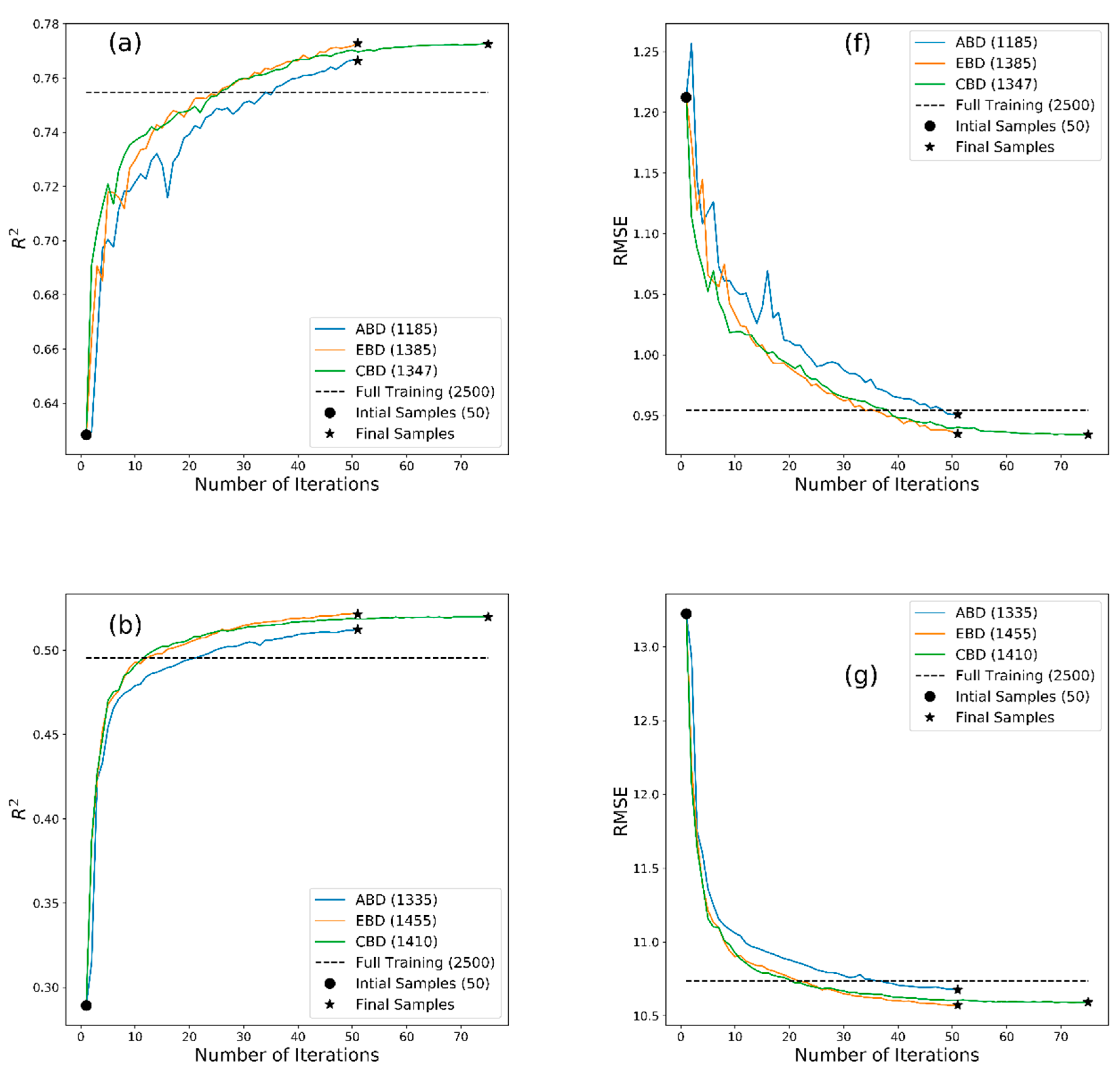
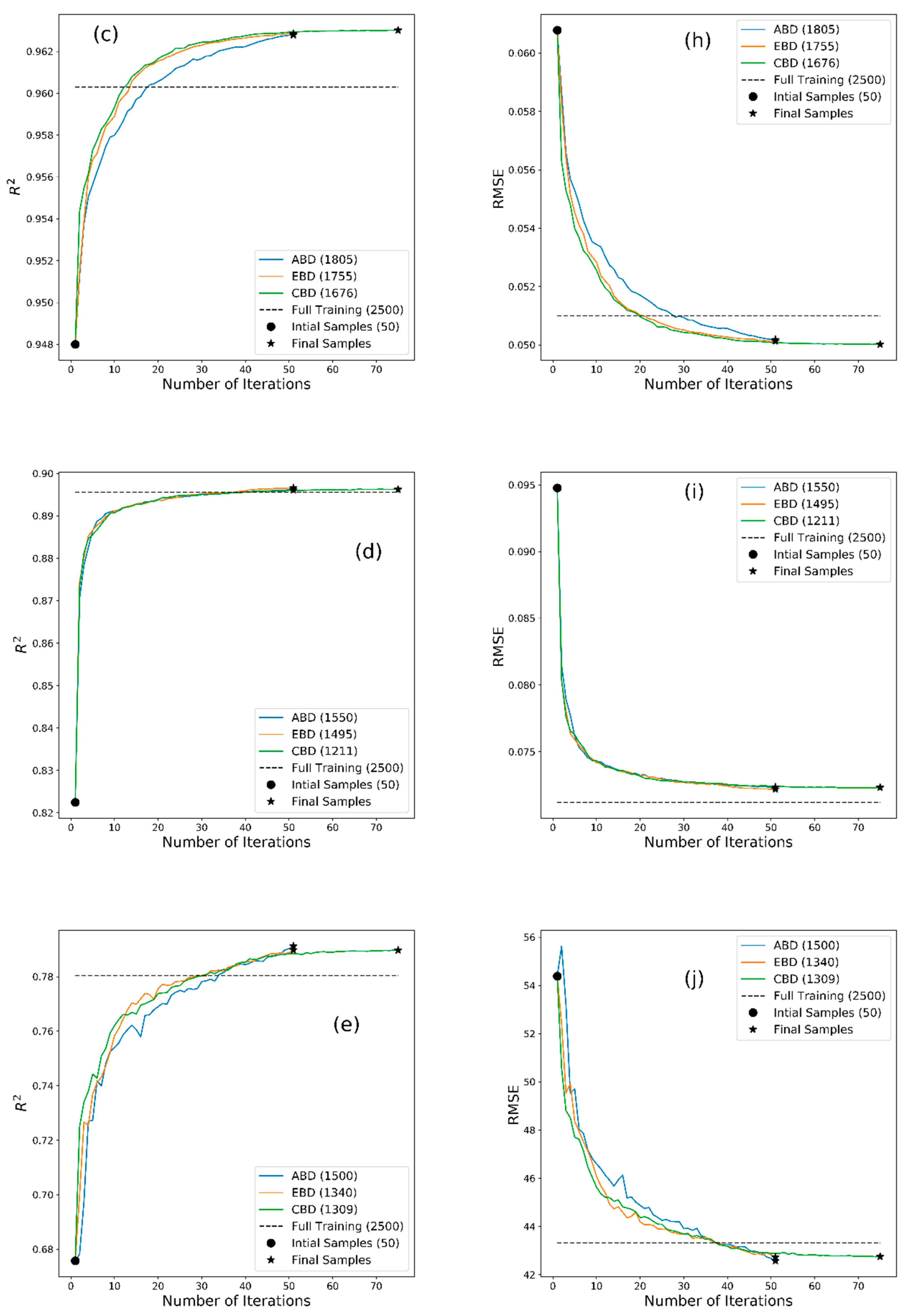
The full simulation dataset generated with PROSAIL was used as a source of subsets for training the different MLAs, as described in the methods section, except for GPR for which a data reduction procedure based on AL was employed. Preliminarily, for GPR we compared three different diversity-based criteria used to perform AL, with respect to the full training with 2500 samples. Figure 2 shows the comparison of the different methods of sample selection in terms of R² and RMSE with respect to the number of iterations, for all the variables, applied to the Maccarese dataset. Only when the performance was improved were the samples added. This explains why fewer samples were added than potentially possible, i.e., less than 50 samples were added for each iteration (e.g., in Figure 2a the final sample size for CBD was of 1347 at 75 iterations).

The Euclidean distance-based diversity metric EBD surpassed ABD and CBD, achieving higher r² and lower RMSE values, i.e., higher accuracy and lower error, with a lower number of samples and iterations. The best performing EBD was thus subsequently used in all further applications of AL in the present work. It should be noted that the training of GPR with the full set of 2500 samples, i.e., without AL, provided worse performance than AL in all cases except for FAPAR, despite using a larger dataset for training, revealing some redundancy in the full set.

In the comparison to all the algorithms tested, the cross-validation metrics give an indication of their performance, though the actual accuracy can be more realistically assessed using ground validation results.

Table 4. Mean RMSE values of the 10 replicates for the estimation of LAI, LCC, CCC, FVC, and FAPAR using different machine learning algorithms (MLRAs) for cross-validation (CV) and ground validation (GV), for the Maccarese test site. Abbreviations for the MLRAs are reported in Table 2. Values sharing the same letters are not significantly different according to Friedman’s aligned rank post-hoc test. The best results for each variable are highlighted in bold.

MLRA	LAI		LCC		CCC		FVC		FAPAR
	CV	GV	CV	GV	CV	GV	CV	GV	CV	GV
BagT	0.99 b	1.01 d	11.4 c	8.90 a	45.83 a,b	46.12 b	0.05 c	0.08 a	0.08 c	0.11 a
NN (ARTMO)	1.04 c	0.90 b	11.02 b	10.68 b,c	46.53 b	52.1 c	0.05 b	0.09 b,c	0.07 b	0.11 a
RFTB	1.00 b	0.93b c	11.55 c,d	8.88 a	46.47 b	44.71 b	0.06 d	0.08 a	0.08 c	0.10 a
PLSR	1.18 e	0.69 a	11.16 b	11.6 c,d	53.25 c	40.44 a	0.06 e	0.13 d	0.09 e	0.12 b
LSLR	1.18 e	0.68 a	11.15 b	12.05 d	53.14 c	40.86 a	0.06 e	0.13 d	0.09 e	0.12 b
BooT	1.14 d	0.98 c,d	11.61 d	10.94 b,c	52.08 c	57.51 c,d	0.06 f	0.09 b	0.08 d	0.11 a
RegT	1.30 f	1.17 e	14.99 e	11.63 c,d	60.26 d	61.22 d,e	0.07 g	0.09 b,c	0.10 f	0.12 b
RFFE	1.40 g	1.44 f	16.03 f	13.18 d	64.36 d	68.32 e	0.08 h	0.10 c	0.11 g	0.12 b
GPR + AL	0.94 a	1.31 f	10.55 a	10.22 b	43.81 a	54.56 c	0.05 a	0.08 a	0.07 a	0.11 a
NN (SNAP)		0.74		10.94		44.61		0.108		0.105

and

Table 5. Mean RMSE values of 10 replicates for the estimation of LAI, LCC, CCC, FVC and FAPAR using different machine learning algorithms (MLRA) for cross-validation (CV) and ground validation (GV), for the Shunyi test site. Abbreviations for the MLRAs are reported in Table 2. Values sharing the same letters are not significantly different according to Friedman’s aligned ranks post-hoc test. The best results for each variable are highlighted in bold.

MLRA	LAI		LCC		CCC		FVC
	CV	GV	CV	GV	CV	GV	CV	GV
BagT	0.99 b	1.74 c,d	11.67 d	17.28 a	46.12 b	56.72 a	0.05 c	0.19 c
NN(ARTMO)	1.02 b	1.42 b	11.27 b	24.41 c	46.52 b	98.14 e	0.05 b	0.17 a
RFTB	1.00 b	1.67 c	11.8 e	16.77 a	46.69 b	56.51 a	0.05 d	0.19 c
PLSR	1.18 d	1.01 a	11.43 c	24.77 c	52.94 c	68.11 c	0.06 f	0.18 b
LSLR	1.18 d	1.00 a	11.43 b,c	25.98 b,c	52.86 c	74.33 d	0.06 f	0.18 b
BooT	1.12 c	1.46 b	11.91 e	25.91 d	51.69 c	94.77 e	0.05 e	0.18 b
RegT	1.32 e	1.76 d	15.26 f	20.75 b	60.63 d	62.71 b	0.07 g	0.21 d
RFFE	1.42 e	2.14 e	16.36 g	25.62 b	64.29 d	76.96 d	0.07 h	0.21 d
GPR + AL	0.93 a	1.98 e	10.79 a	22.75 b	42.55 a	61.35 b	0.05 a	0.18 b
NN (SNAP)		1.16		23.61		123.53		0.18

report the summary of RMSE estimates for both cross-validation and ground validation for the Maccarese and Shunyi datasets, respectively, for all the algorithms tested.

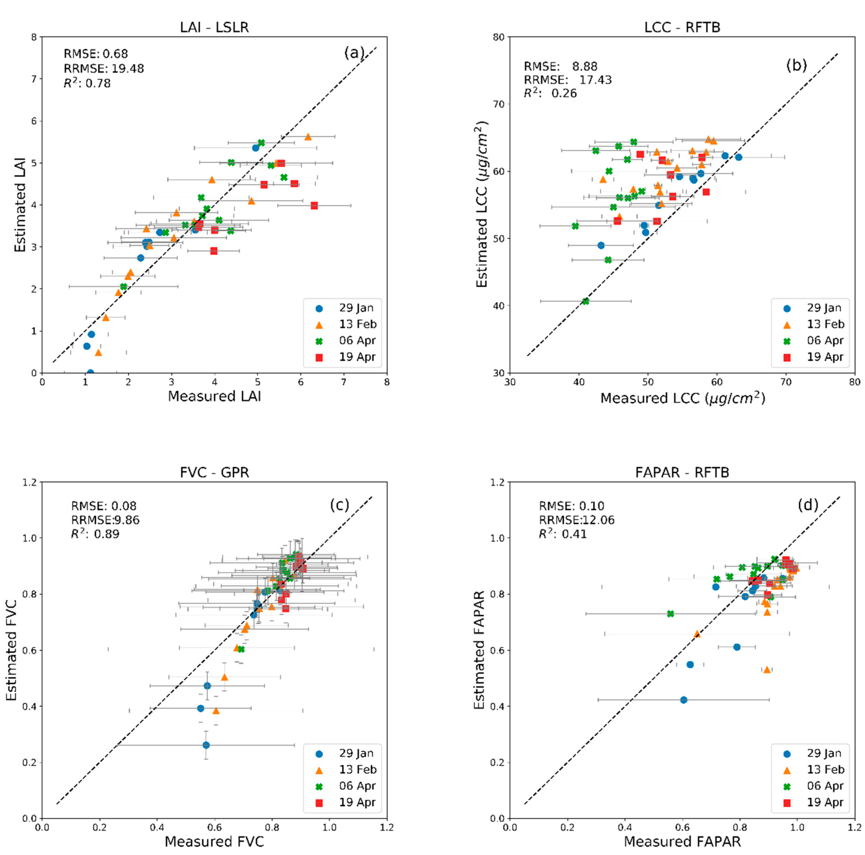
For Maccarese (Table 4), LSLR and PLSR were the best performing algorithms for LAI retrieval when validated with ground data, in terms of RMSE, with values of 0.68 (R² = 0.78, RRMSE = 19.48%) and 0.69 (R² = 0.78, RRMSE = 19.84%) respectively. These were also the fastest computing algorithms among all the MLRAs in terms of time required for training (data not shown). The cross-validation and ground validation results (Figure 3a) indicated that LSLR apparently did not show saturation, even up to LAI values of 5 or 6. The retrieval of LCC was best performed by RFTB (Figure 3b) and BagT, with RMSE values of 8.88 μg cm⁻² (R² = 0.26 and RRMSE = 17.43%) and 8.90 μg cm⁻² (R² = 0.27 and RRMSE = 17.46%). 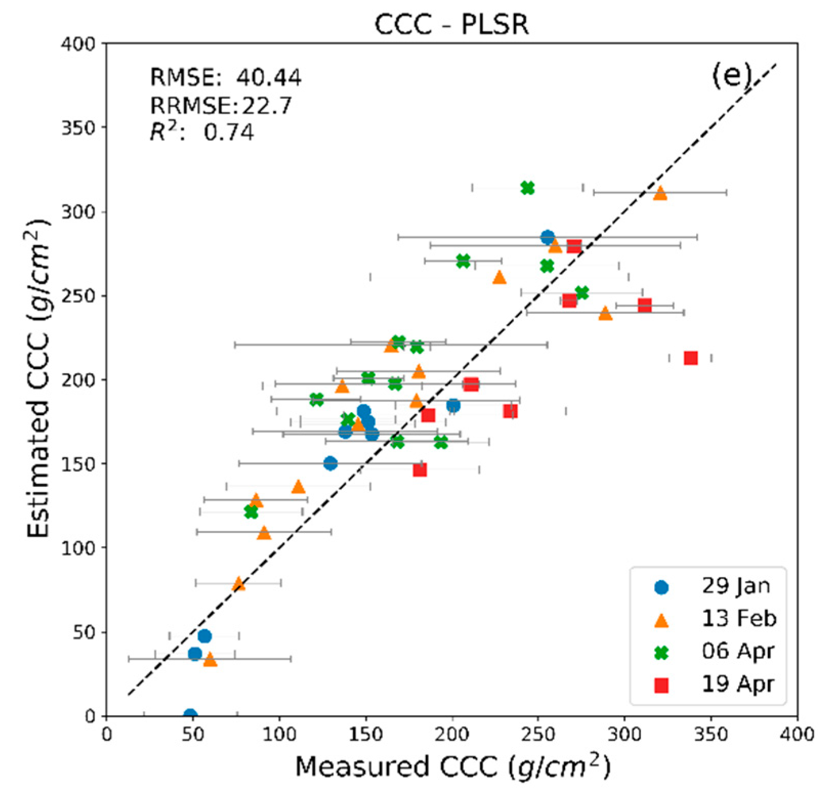An overestimation of LCC was observed (Figure 3b). The lowest RMSE of 40.44 g cm⁻² (R² = 0.74 RRMSE = 22.7%) (Figure 3e), was obtained for the retrieval of CCC with PLSR. The retrieval accuracy of LSLR was not significantly different from that of PLSR for CCC (RMSE = 40.86 g cm⁻², R² = 0.74 and RRMSE = 22.9%). Indeed, PLSR was not significantly different from LSLR in terms of RMSE for all the variables considered. The lowest RMSE for FVC was 0.08 (R² = 0.9 and RRMSE = 9.8%), obtained with the GPR algorithm (Figure 3c). For FVC, RFTB and BagT were also not significantly different from GPR in terms of RMSE. The FAPAR was best retrieved with a RMSE of 0.10 (R² = 0.41 and RRMSE = 12.06%) using the RFTB approach (Figure 3d), although GPR was not significantly different in terms of RMSE, which was only slightly higher. It was observed that, even in the best performing algorithms, an underestimation of low values of FVC and FAPAR was apparent (Figure 3c,d). It should also be noted that these latter variables show a smaller range of variation in the measured values as compared to the other biophysical variables. As can be seen, GPR was always the best performing algorithm in the cross-validation results, but this was not confirmed by the ground validation tests, with the exception of FVC and FAPAR estimation.

As can be observed from the horizontal error bars of Figure 3, considerable variability occurred among ground measurements inside ESUs, despite the visually apparent homogeneity of the crop canopy in the sampled area of each ESU.

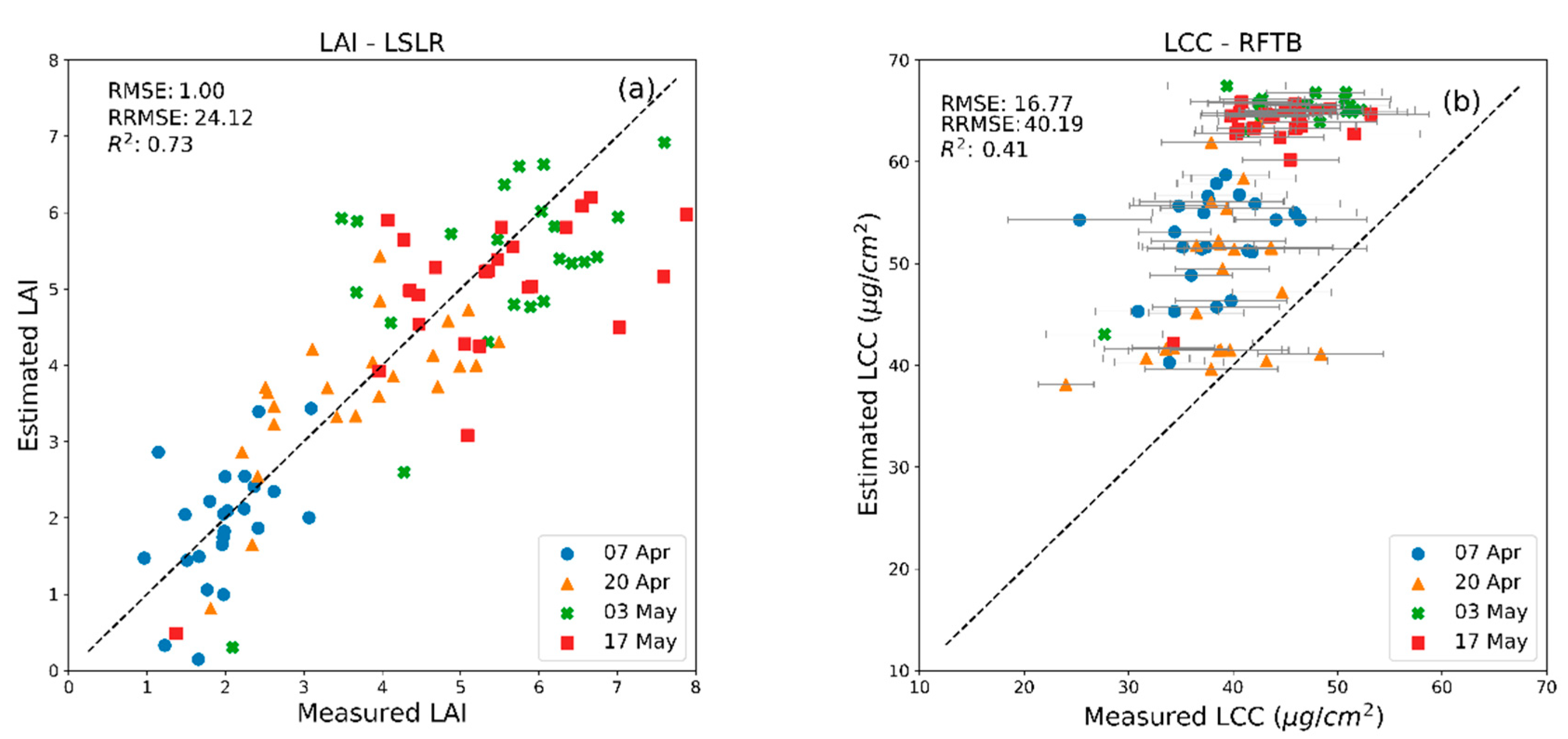
For the Shunyi datasets (Table 5), the ground variability could not be reported for LAI, for which single-point measurements were carried out, but an estimate of the variability for chlorophyll could be made since multiple measurements were available for each point (Figure 4b).

The best accuracy for LAI retrieval for the Shunyi site was a RMSE of 1.00 m² m⁻² (R² = 0.73 and RRMSE = 24.12%) obtained with LSLR (Table 5), i.e., the same algorithm providing the best results also for Maccarese. For LAI, PLSR had a similar performance as that of LSLR, with a RMSE = 1.01 m² m⁻² and (R² = 0.72 and RRMSE = 24.50%), i.e., also consistently with the results of LAI retrieval for Maccarese. Similarly, for Maccarese, LCC was best retrieved with an RMSE value of 16.77 μg cm⁻², (R² = 0.41 and RRMSE = 40.19%) using RFTB (Table 5). 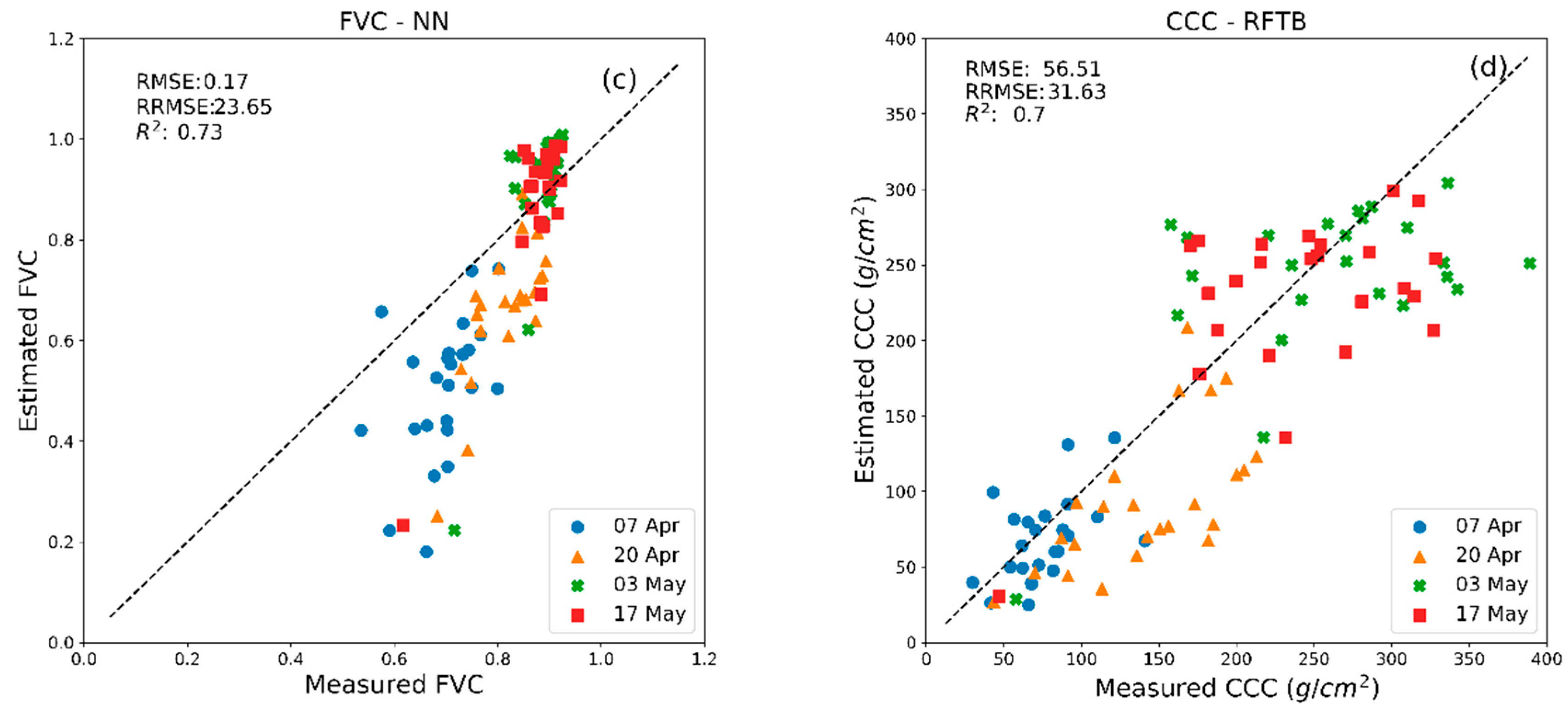Although RFTB produced the lowest error for retrieving LCC, its retrieval using BagT approach was not significantly different, with RMSE = 17.28 μg cm⁻², R² = 0.41 and RRMSE = 41.41%. For CCC retrieval, the lowest RMSE, 56.51 g cm⁻² (R² = 0.7, RRMSE = 31.63%), was achieved by the RFTB method. In this case, BagT was not significantly different from RFTB (R² = 0.71, RMSE = 56.72 and RRMSE = 31.75%). For this test site, FVC was retrieved with an RMSE of 0.17 (R² = 0.73 and RRMSE = 23.65%) with NNs (Figure 4c). Also, for the Shunyi test site, GPR was always the best performing algorithm in cross-validation but not in ground validation tests.

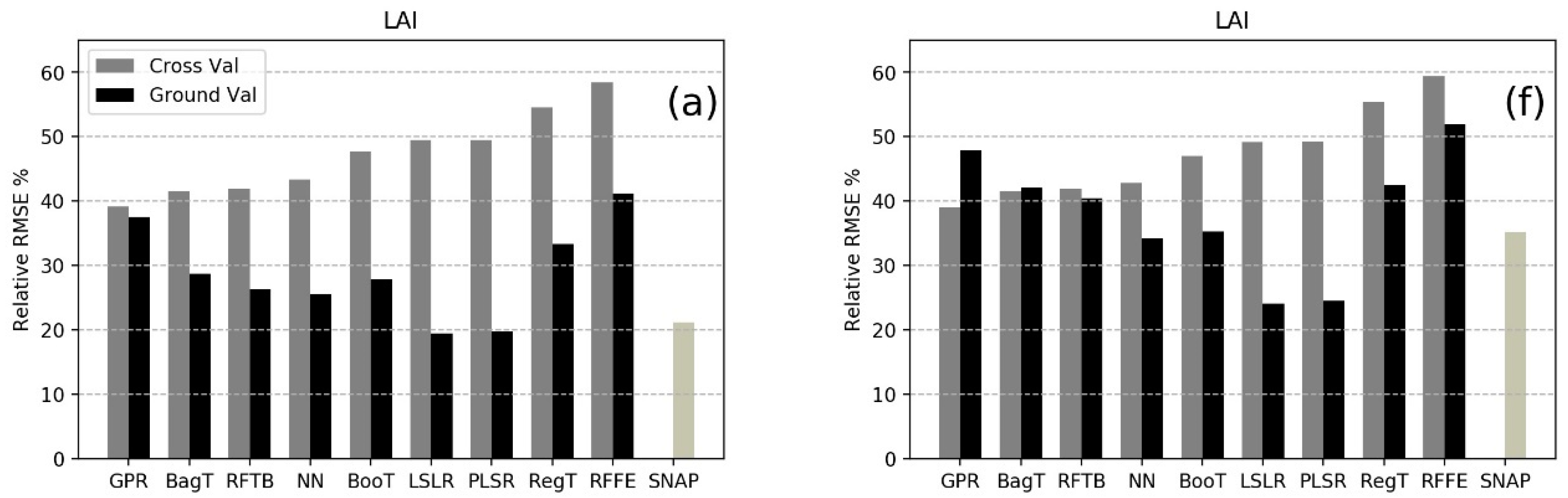
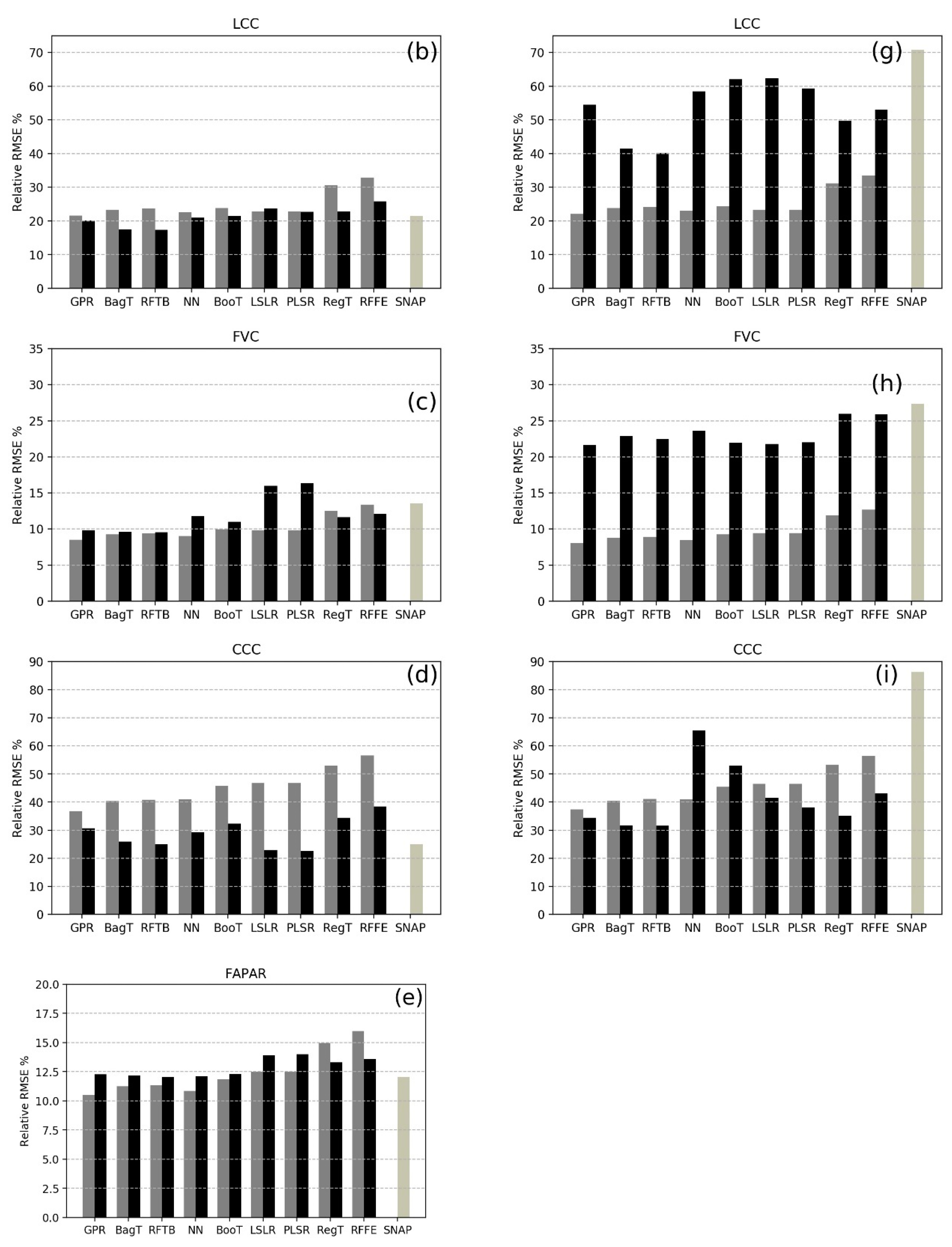
A summary of the results in terms of RRMSE for all the biophysical variables tested with different MLRAs for both sites is presented in Figure 5.

It can be seen from Figure 5, that the k-fold cross-validation (k = 10) provided in some circumstances worse results (higher RRMSE) than the validation with ground data (e.g., Figure 5a). This is particularly evident for LAI and CCC for the Maccarese site. Usually, since it was carried out with subset of the same dataset as used for the training of the MLRAs, the cross-validation error was lower than the ground validation error, but this was not the case here, as can be seen from Figure 5a–e. The different statistical distributions of training and ground validation data might be a possible reason. It appears that the range of variation of the training sets was much larger than that of the ground validation sets, with more extreme values. This could have possibly led to more unreliable retrievals in the cross-validation when extreme values were sampled, which did not happen in the ground validation.

For the Shunyi test site, RRMSE values were generally higher than for the Maccarese (Figure 5), probably because of the larger differences in the statistical distributions of the ground validation dataset from the training set, as compared for the Maccarese and possibly for the larger error introduced by the sampling protocol.

In general, for LAI, algorithms such as LSLR and PLSR, seemed to outperform more complex MLRAs such as NNs, for example providing better results than those found by applying the biophysical processor implemented in the ESA SNAP toolbox.

For leaf chlorophyll (LCC), much worse results were obtained for Shunyi than for Maccarese, with a clear advantage of RFTB for both sites for ground validation tests. The performance of the NN implementation of SNAP was particularly poor for Shunyi, though it should be noted that this variable was back-calculated from the CCC variable generated by SNAP.

Fractional ground cover (FVC) showed the smallest error among all the biophysical variables tested, alongside FAPAR which was only available for Maccarese. Neural networks provided the best accuracies with the lowest values of relative RMSEs for the latter variable.

Although different algorithms from different families of MLRAs performed well for different biophysical variables, the GPR was considered particularly interesting, as it provided uncertainty estimates with the mean value of prediction (Figure 3c). However, despite its good cross-validation results, GPR ranked as the top algorithm only for FVC and FAPAR for the Maccarese test site (Table 4). The AL procedure only selected the most informative samples of the dataset, thus the training of GPR was performed with a smaller set of PROSAIL simulations compared to the other algorithms, showing that it was quite efficient and robust.

The time taken for training the models ranged from 0.003 seconds for LSLR to 47.5 seconds for NNs and a maximum 548.3 seconds for GPR. Although, GPR took longer to train, it should be noted that it performed AL using EBD and used fewer samples to train and achieved high accuracy in comparison to other models.

When considering single ground sampling dates separately, generally the retrieval performances were improved (

Table 6. Ground validation estimation results at each ground sampling date, for the best performing algorithms for the Maccarese test site.

MLRA	29 January 2018		13 February 2018		6 April 2018		20 April 2018
	R2	RMSE	R2	RMSE	R2	RMSE	R2	RMSE
LSLR (LAI)	0.89	0.59	0.88	0.55	0.73	0.51	0.55	1.09
RFTB (LCC)	0.91	3.01	0.55	7.75	0.25	12.56	0.11	7.03
GPR (FVC)	0.90	0.12	0.89	0.08	0.90	0.05	0.71	0.05
RFTB (FAPAR)	0.74	0.10	0.45	0.14	0.44	0.09	0.56	0.06
PLSR (CCC)	0.94	26.32	0.87	33.37	0.65	44.46	0.45	55.97

) compared to the bulked data (Table 4). In some cases, e.g., LAI and CCC, the worst results were obtained at the latest date, due to the fact that it was generally more difficult to estimate higher LAI values.

4. Discussion

There are different methods for the retrieval of biophysical variables from remote sensing data and all the methods have their pros and cons [16]. Currently, hybrid methods have the capability of combining physical and statistical methods and are considered state of the art. In this paper, different MLRAs (kernel-based and non-kernel based) were trained and applied for the retrieval of the crop biophysical variables LAI, LCC, FAPAR, FVC, and CCC with the same configuration and settings of RTM PROSAIL simulated spectra as those implemented in ESA SNAP biophysical variables retrieval toolbox, with the exception of the observation geometry. With the same of configuration of PROSAIL parameters (Section 2.1), a total of 41,472 simulated spectra was generated, which turned out to be rather redundant and inefficient for performing the training steps. Subsets of 2500 randomly extracted simulated spectra were used to perform the training of the algorithms and this procedure was repeated ten times with different subsets. This was done in order to allow a comparison of alternative MLRAs to a well-established operational algorithm [29].

The SNAP algorithm relies on the use of PROSAIL simulations for training NNs, which are the most widely-used tools for operational biophysical variables retrieval [25,26,27,28]. The downside of the NNs are that they require a relatively long time for training, tuning of parameters is a difficult task, they are black box in nature, and can be unpredictable if training and validation data deviate from each other even slightly [5]. In this paper, various alternative MLRAs outperformed NNs. For example, LAI retrieval was best performed with LSLR and PLSR, consistently for both tests, although with different accuracies, i.e., RMSE of 0.68 for Maccarese and 1 for Shunyi [5], compared with different retrieval strategies for LAI and reporting the best performing algorithms for each category. In the case of parametric regression, the best performing algorithm was Tian 3-band formulation (RMSE = 0.615 and R² = 0.823), whereas VH-GPR performed best among non-parametric regression algorithms (RMSE = 0.436 and R² = 0.902). However, it should be noted that the accuracies found by these authors, somehow better than those of the present study, could be explained by the fact that they used cross-validation in which the training was carried out using the ground dataset, not independent model simulations such as in the present work.

The LCC was best retrieved by the RFTB method for both sites, revealing a general overestimation, but the error of estimation was higher for the Shunyi test site compared to the Maccarese (Figure 3b and Figure 4b), particularly for SNAP. Also, the error of CCC estimates was very high for the SNAP tool compared to the other algorithms tested in this work for the Shunyi ground validation (Figure 5i). It was previously shown by Reference [64] that Sentinel-2 bands at a 10 m spatial resolution are suitable for estimating LAI, LCC, and CCC. They retrieved LAI (R² = 0.809), LCC (R² = 0.696) and CCC (R² = 0.818) with vegetation indices approach. Multiple vegetation indices were compared for identification of potential vegetation index for the retrieval of LAI, LCC, and CCC in [65], the best correlation for LCC was with the Meris Terrestrial Chlorophyll Index (MTCI) (R² = 0.77) and Sentinel-2 red-edge position index (S2REP) (R² = 0.91), for LAI, inverted red-edge chlorophyll index (IRECI) (R² = 0.77) and NDI45 (R² = 0.62), Normalised Difference Vegetation Index (NDVI) for CCC (R² = 0.70). These results are better than those found in the present work, but again, empirical approaches employing the ground datasets were employed by these authors for the calibration of the models.

The FVC variable was more accurately predicted than LAI or LCC, though with slightly higher error for Shunyi. With hierarchical tree-based methods such as BagT, RFTB, and GPR, the error reached was even lower than 10%, which is in line with Global Monitoring for Environment and Security (GMES) goal accuracy [66] (Figure 5c). In the case of CCC retrieval, it can be noted that the lowest RRMSE was provided by RFTB and BagT, though also GPR performs similarly to RFTB. The FAPAR variable was only estimated for the Maccarese test site, due to the unavailability of the ground measurements for validation, it was not estimated for the Shunyi test site. The results showed that this variable was best retrieved with the RFTB method, with the lowest RMSE (Table 3).

The GPR was proved to be an efficient and powerful regressor for the biophysical variables retrieval in previous reports [18]. A study conducted by Reference [18], retrieved LAI, Chl, and FVC using different methods, such as NNs, kernel ridge regression (KRR), support vector regression, and GPR for different Sentinel-2 and Sentinel-3 configurations. They found that an overall good performance throughout all Sentinel configurations was provided by GPR. A study carried out by Reference [10] also found that GPR using AL techniques is an efficient and robust method for the retrieval of LAI and LCC from Sentinel-3 OLCI spectra. However, this was not the case in our study. The GPR method, coupled with AL procedure, provided the best results in terms of computational time and low error only for FVC and FAPAR ground validation tests (Figure 5c,e,h). On the other hand, GPR generally performed as the best algorithm for the retrieval of all the biophysical variables, only for the cross-validations tests (Table 4 and Table 5). Hence, of importance for further analysis to investigate how accurately GPR performs when validated against independent ground data. As Reference [10] pointed out, GPR is based on non-parametric regression in a Bayesian framework, it provides insights in bands carrying relevant information and also in theoretical uncertainty estimates, thus partially overcoming the black box problem [5]. These uncertainties are a useful tool for the assessment of upscaling capabilities of biophysical variables from airborne or spaceborne platforms and their respective scales [32]. A study conducted by [9] introduced the AL approach with GPR and SVM regressions to deal with the problems of training sample collection for biophysical variables estimation. Their results obtained on simulated MEdium Resolution Imaging Spectrometer (MERIS) and real SeaWiFS Bio-optical Algorithm Mini-Workshop (SeaBAM) datasets were characterized by higher performances in terms of both accuracy and stability with respect to a completely random selection strategy. The present work seems to support these results highlighting the efficiency of the AL procedure, since, when using a smaller set of selected training data, comparable results were obtained than with a random selection of larger size (Figure 2).

5. Conclusions

Hybrid methods of biophysical variables retrieval rely on the generation of simulated spectra using physically-based RTM for the training of MLRAs, under the assumption of a more general applicability as compared to the training carried out using measured data, since RTMs allow to simulate a wider range of leaf and canopy properties. Operationally, so far, only NNs have been implemented as a hybrid method, e.g., in the ESA SNAP toolbox. Due to complexity of parameter tuning and the black box nature of the algorithm, in recent years, several studies have focused on alternative MLRAs such as kernel-based methods. They offer an interesting alternative to NNs in terms of performance and computational demand, sometimes partially overcoming the black box nature of NNs. In the present study, it was shown, using the same set of PROSAIL simulations, that some MLRAs could provide better results than NN-based algorithms implemented in SNAP. This was particularly evident for chlorophyll and fractional vegetation cover. It resulted that the best performing algorithms varied according to the biophysical variables to be estimated: e.g., LSLR and PLSR worked better for LAI, whereas RFTB and BagT for LCC. This study also showed that these variables’ results were consistent for two different datasets respectively collected in Italy and China on wheat, though the retrieval accuracies depended somehow on errors introduced during the ground sampling protocol. The absolute values of the retrieval accuracies are in some cases higher than the best performances reported in previous studies, but most of these previous studies did not train the regression algorithms with completely independent datasets, as was done in the present study. Further studies should be conducted to investigate alternative strategies, e.g., of active learning procedures, using different kernel functions, and validate the retrievals using a wider range of agricultural crops, also assessing their performance for canopies that depart more from the assumptions of the turbid medium used in the PROSAIL RTM.

References

1. Zhang, C.; Kovacs, J.M. The application of small unmanned aerial systems for precision agriculture: A review. Precis. Agric. 2012, 13, 693–712. [Google Scholar] [CrossRef]
2. Jay, S.; Maupas, F.; Bendoula, R.; Gorretta, N. Retrieving LAI, chlorophyll and nitrogen contents in sugar beet crops from multi-angular optical remote sensing: Comparison of vegetation indices and PROSAIL inversion for field phenotyping. Field Crops Res. 2017, 210, 33–46. [Google Scholar] [CrossRef] [Green Version]
3. Goffart, J.P.; Olivier, M.; Frankinet, M. Potato crop nitrogen status assessment to improve N fertilization management and efficiency: Past–present–future. Potato Res. 2008, 51, 355–383. [Google Scholar] [CrossRef]
4. Cilia, C.; Panigada, C.; Rossini, M.; Meroni, M.; Busetto, L.; Amaducci, S.; Boschetti, M.; Picchi, V.; Colombo, R. Nitrogen status assessment for variable rate fertilization in maize through hyperspectral imagery. Remote Sens. 2014, 6, 6549–6565. [Google Scholar] [CrossRef]
5. Verrelst, J.; Rivera, J.P.; Veroustraete, F.; Muñoz-Marí, J.; Clevers, J.G.; Camps-Valls, G.; Moreno, J. Experimental Sentinel-2 LAI estimation using parametric, non-parametric and physical retrieval methods–A comparison. ISPRS J. Photogramm. Remote Sens. 2015, 108, 260–272. [Google Scholar] [CrossRef]
6. Jordan, C.F. Derivation of leaf-area index from quality of light on the forest floor. Ecology 1969, 50, 663–666. [Google Scholar] [CrossRef]
7. Rouse, J.; Haas, R.; Schell, J.; Deering, D.; Harlan, J. Monitoring the Vernal Advancement of Retrogradation of Natural Vegetation, NASA/GSFC, Type III, Final Report. Available online: https://ntrs.nasa.gov/archive/nasa/casi.ntrs.nasa.gov/19730017588.pdf (accessed on 20 February 2019).
8. Rondeaux, G.; Steven, M.; Baret, F. Optimization of soil-adjusted vegetation indices. Remote Sens. Environ. 1996, 55, 95–107. [Google Scholar] [CrossRef]
9. Pasolli, E.; Melgani, F.; Alajlan, N.; Bazi, Y. Active learning methods for biophysical parameter estimation. IEEE Trans. Geosci. Remote Sens. 2012, 50, 4071–4084. [Google Scholar] [CrossRef]
10. Verrelst, J.; Dethier, S.; Rivera, J.P.; Muñoz-Marí, J.; Camps-Valls, G.; Moreno, J. Active learning methods for efficient hybrid biophysical variable retrieval. IEEE Geosci. Remote Sens. Lett. 2016, 13, 1012–1016. [Google Scholar] [CrossRef]
11. Verrelst, J.; Camps-Valls, G.; Muñoz-Marí, J.; Rivera, J.P.; Veroustraete, F.; Clevers, J.G.; Moreno, J. Optical remote sensing and the retrieval of terrestrial vegetation bio-geophysical properties–A review. ISPRS J. Photogramm. Remote Sens. 2015, 108, 273–290. [Google Scholar] [CrossRef]
12. Pignatti, S.; Acito, N.; Amato, U.; Casa, R.; Castaldi, F.; Coluzzi, R.; De Bonis, R.; Diani, M.; Imbrenda, V.; Laneve, G.; et al. Environmental products overview of the Italian hyperspectral prisma mission: The SAP4PRISMA project. In Proceedings of the 2015 IEEE International Geoscience and Remote Sensing Symposium (IGARSS), Milan, Italy, 26–31 July 2015. [Google Scholar]
13. Guanter, L.; Kaufmann, H.; Segl, K.; Foerster, S.; Rogass, C.; Chabrillat, S.; Kuester, T.; Hollstein, A.; Rossner, G.; Chlebek, C. The EnMAP spaceborne imaging spectroscopy mission for earth observation. Remote Sens. 2015, 7, 8830–8857. [Google Scholar] [CrossRef]
14. Durbha, S.S.; King, R.L.; Younan, N.H. Support vector machines regression for retrieval of leaf area index from multiangle imaging spectroradiometer. Remote Sens. Environ. 2007, 107, 348–361. [Google Scholar] [CrossRef]
15. Lázaro-Gredilla, M.; Titsias, M.K.; Verrelst, J.; Camps-Valls, G. Retrieval of biophysical parameters with heteroscedastic Gaussian processes. IEEE Geosci. Remote Sens. Lett. 2014, 11, 838–842. [Google Scholar] [CrossRef]
16. Verrelst, J.; Malenovský, Z.; Van der Tol, C.; Camps-Valls, G.; Gastellu-Etchegorry, J.-P.; Lewis, P.; North, P.; Moreno, J. Quantifying Vegetation Biophysical Variables from Imaging Spectroscopy Data: A Review on Retrieval Methods. Surv. Geophys. 2018, 1–41. (in press). [Google Scholar] [CrossRef]
17. Knudby, A.; LeDrew, E.; Brenning, A. Predictive mapping of reef fish species richness, diversity and biomass in Zanzibar using IKONOS imagery and machine-learning techniques. Remote Sens. Environ. 2010, 114, 1230–1241. [Google Scholar] [CrossRef]
18. Verrelst, J.; Muñoz, J.; Alonso, L.; Delegido, J.; Rivera, J.P.; Camps-Valls, G.; Moreno, J. Machine learning regression algorithms for biophysical parameter retrieval: Opportunities for Sentinel-2 and-3. Remote Sens. Environ. 2012, 118, 127–139. [Google Scholar] [CrossRef]
19. Wang, L.; Zhou, X.; Zhu, X.; Dong, Z.; Guo, W. Estimation of biomass in wheat using random forest regression algorithm and remote sensing data. Crop J. 2016, 4, 212–219. [Google Scholar] [CrossRef] [Green Version]
20. Benítez, J.M.; Castro, J.L.; Requena, I. Are artificial neural networks black boxes? IEEE Trans. Neural Netw. 1997, 8, 1156–1164. [Google Scholar] [CrossRef] [PubMed] [Green Version]
21. Rivera, J.P.; Verrelst, J.; Leonenko, G.; Moreno, J. Multiple cost functions and regularization options for improved retrieval of leaf chlorophyll content and LAI through inversion of the PROSAIL model. Remote Sens. 2013, 5, 3280–3304. [Google Scholar] [CrossRef]
22. Combal, B.; Baret, F.; Weiss, M.; Trubuil, A.; Mace, D.; Pragnere, A.; Myneni, R.; Knyazikhin, Y.; Wang, L. Retrieval of canopy biophysical variables from bidirectional reflectance: Using prior information to solve the ill-posed inverse problem. Remote Sens. Environ. 2003, 84, 1–15. [Google Scholar] [CrossRef]
23. Atzberger, C. Object-based retrieval of biophysical canopy variables using artificial neural nets and radiative transfer models. Remote Sens. Environ. 2004, 93, 53–67. [Google Scholar] [CrossRef]
24. Houborg, R.; Boegh, E. Mapping leaf chlorophyll and leaf area index using inverse and forward canopy reflectance modeling and SPOT reflectance data. Remote Sens. Environ. 2008, 112, 186–202. [Google Scholar] [CrossRef]
25. Pozdnyakov, D.; Shuchman, R.; Korosov, A.; Hatt, C. Operational algorithm for the retrieval of water quality in the Great Lakes. Remote Sens. Environ. 2005, 97, 352–370. [Google Scholar] [CrossRef]
26. Schiller, H.; Doerffer, R. Improved determination of coastal water constituent concentrations from MERIS data. IEEE Trans. Geosci. Remote Sens. 2005, 43, 1585–1591. [Google Scholar] [CrossRef]
27. Verger, A.; Baret, F.; Weiss, M. Performances of neural networks for deriving LAI estimates from existing CYCLOPES and MODIS products. Remote Sens. Environ. 2008, 112, 2789–2803. [Google Scholar] [CrossRef]
28. Verger, A.; Baret, F.; Camacho, F. Optimal modalities for radiative transfer-neural network estimation of canopy biophysical characteristics: Evaluation over an agricultural area with CHRIS/PROBA observations. Remote Sens. Environ. 2011, 115, 415–426. [Google Scholar] [CrossRef]
29. Weiss, M.; Baret, F. S2ToolBox Level 2 Products: LAI, FAPAR, FCOVER. Available online: https://step.esa.int/docs/extra/ATBD_S2ToolBox_L2B_V1.1.pdf (accessed on 21 February 2019).
30. Chai, L.; Qu, Y.; Zhang, L.; Wang, J. Lai retrieval from cyclopes and modis products using artificial neural networks. In Proceedings of the 2008 Geoscience and Remote Sensing Symposium, Boston, MA, USA, 7–11 July 2008. [Google Scholar]
31. Camps-Valls, G.; Bruzzone, L. Kernel Methods for Remote Sensing Data Analysis; John Wiley & Sons: Hoboken, NJ, USA, 2009. [Google Scholar]
32. Verrelst, J.; Alonso, L.; Caicedo, J.P.R.; Moreno, J.; Camps-Valls, G. Gaussian process retrieval of chlorophyll content from imaging spectroscopy data. IEEE J. Sel. Top. Appl. Earth Obs. Remote Sens. 2013, 6, 867–874. [Google Scholar] [CrossRef]
33. Verrelst, J.; Rivera, J.P.; Moreno, J.; Camps-Valls, G. Gaussian processes uncertainty estimates in experimental Sentinel-2 LAI and leaf chlorophyll content retrieval. ISPRS J. Photogramm. Remote Sens. 2013, 86, 157–167. [Google Scholar] [CrossRef]
34. Verrelst, J.; Rivera, J.P.; Gitelson, A.; Delegido, J.; Moreno, J.; Camps-Valls, G. Spectral band selection for vegetation properties retrieval using Gaussian processes regression. Int. J. Appl. Earth Obs. Geoinf. 2016, 52, 554–567. [Google Scholar] [CrossRef]
35. Settles, B. Active Learning Literature Survey. Available online: http://burrsettles.com/pub/settles.activelearning.pdf (accessed on 21 January 2019).
36. Gascon, F.; Bouzinac, C.; Thépaut, O.; Jung, M.; Francesconi, B.; Louis, J.; Lonjou, V.; Lafrance, B.; Massera, S.; Gaudel-Vacaresse, A. Copernicus Sentinel-2A calibration and products validation status. Remote Sens. 2017, 9, 584. [Google Scholar] [CrossRef]
37. Jacquemoud, S.; Verhoef, W.; Baret, F.; Bacour, C.; Zarco-Tejada, P.J.; Asner, G.P.; François, C.; Ustin, S.L. PROSPECT+ SAIL models: A review of use for vegetation characterization. Remote Sens. Environ. 2009, 113, S56–S66. [Google Scholar] [CrossRef]
38. Feret, J.-B.; François, C.; Asner, G.P.; Gitelson, A.A.; Martin, R.E.; Bidel, L.P.; Ustin, S.L.; Le Maire, G.; Jacquemoud, S. PROSPECT-4 and 5: Advances in the leaf optical properties model separating photosynthetic pigments. Remote Sens. Environ. 2008, 112, 3030–3043. [Google Scholar] [CrossRef]
39. Verhoef, W. Light scattering by leaf layers with application to canopy reflectance modeling: The SAIL model. Remote Sens. Environ. 1984, 16, 125–141. [Google Scholar] [CrossRef] [Green Version]
40. Meroni, M.; Colombo, R.; Panigada, C. Inversion of a radiative transfer model with hyperspectral observations for LAI mapping in poplar plantations. Remote Sens. Environ. 2004, 92, 195–206. [Google Scholar] [CrossRef]
41. Richter, K.; Atzberger, C.; Vuolo, F.; Weihs, P.; d’Urso, G. Experimental assessment of the Sentinel-2 band setting for RTM-based LAI retrieval of sugar beet and maize. Can. J. Remote Sens. 2009, 35, 230–247. [Google Scholar] [CrossRef]
42. Richter, R.; Schlapfer, D.; Muller, A. Operational atmospheric correction for imaging spectrometers accounting for the smile effect. IEEE Trans. Geosci. Remote Sens. 2011, 49, 1772–1780. [Google Scholar] [CrossRef]
43. Palacharla, P.K.; Durbha, S.S.; King, R.L.; Gokaraju, B.; Lawrence, G.W. A hyperspectral reflectance data based model inversion methodology to detect reniform nematodes in cotton. In Proceedings of the 6th International Workshop on the Analysis of Multi-Temporal Remote Sensing Images (Multi-Temp), Trento, Italy, 12–14 July 2011. [Google Scholar]
44. Le Maire, G.; Marsden, C.; Verhoef, W.; Ponzoni, F.J.; Seen, D.L.; Bégué, A.; Stape, J.-L.; Nouvellon, Y. Leaf area index estimation with MODIS reflectance time series and model inversion during full rotations of Eucalyptus plantations. Remote Sens. Environ. 2011, 115, 586–599. [Google Scholar] [CrossRef]
45. Si, Y.; Schlerf, M.; Zurita-Milla, R.; Skidmore, A.; Wang, T. Mapping spatio-temporal variation of grassland quantity and quality using MERIS data and the PROSAIL model. Remote Sens. Environ. 2012, 121, 415–425. [Google Scholar]
46. Liang, L.; Qin, Z.; Zhao, S.; Di, L.; Zhang, C.; Deng, M.; Lin, H.; Zhang, L.; Wang, L.; Liu, Z. Estimating crop chlorophyll content with hyperspectral vegetation indices and the hybrid inversion method. Int. J. Remote Sens. 2016, 37, 2923–2949. [Google Scholar] [CrossRef]
47. Bacour, C.; Jacquemoud, S.; Tourbier, Y.; Dechambre, M.; Frangi, J.-P. Design and analysis of numerical experiments to compare four canopy reflectance models. Remote Sens. Environ. 2002, 79, 72–83. [Google Scholar] [CrossRef]
48. Baret, F.; Hagolle, O.; Geiger, B.; Bicheron, P.; Miras, B.; Huc, M.; Berthelot, B.; Niño, F.; Weiss, M.; Samain, O.; et al. LAI, fAPAR and fCover CYCLOPES global products derived from VEGETATION. Remote Sens. Environ. 2007, 110, 275–286. [Google Scholar] [CrossRef] [Green Version]
49. Bajwa, S.G.; Gowda, P.H.; Howell, T.A.; Leh, M. Comparing Artificial Neural Network and Least Square Regression Techniques for LAI Retrieval from Remote Sensing Data. Available online: http://www.asprs.org/a/publications/proceedings/pecora17/0006.pdf (accessed on 21 February 2019).
50. Geladi, P.; Kowalski, B.R. Partial least-squares regression: A tutorial. Anal. Chim. Acta 1986, 185, 1–17. [Google Scholar] [CrossRef]
51. Hagan, M.T.; Menhaj, M.B. Training feedforward networks with the Marquardt algorithm. IEEE Trans. Neural Netw. 1994, 5, 989–993. [Google Scholar] [CrossRef] [PubMed]
52. Breiman, L.; Friedman, J.H.; Olshen, R.A.; Stone, C.J. Classification and Regression Trees; Routledge: New York, NY, USA, 1984. [Google Scholar]
53. Friedman, J.; Hastie, T.; Tibshirani, R. Additive logistic regression: A statistical view of boosting (with discussion and a rejoinder by the authors). Ann. Stat. 2000, 28, 337–407. [Google Scholar] [CrossRef]
54. Breiman, L. Bagging predictors. Mach. Learn. 1996, 24, 123–140. [Google Scholar] [CrossRef] [Green Version]
55. Breiman, L. Random forests. Mach. Learn. 2001, 45, 5–32. [Google Scholar] [CrossRef]
56. Williams, C.K.; Rasmussen, C.E. Gaussian Processes for Machine Learning. Available online: http://www.gaussianprocess.org/gpml/chapters/RW.pdf (accessed on 20 February 2019).
57. Williams, C.K.; Rasmussen, C.E. Gaussian Processes for Regression. Available online: https://pdfs.semanticscholar.org/e251/664b68fe1b2bdbf39d938b96adfabe54c4fd.pdf (accessed on 20 February 2019).
58. Verrelst, J.; Rivera, J.; Alonso, L.; Moreno, J. ARTMO: An Automated Radiative Transfer Models Operator Toolbox for Automated Retrieval of Biophysical Parameters Through Model Inversion. Available online: http://ipl.uv.es/artmo/files/JV_ARTMO_paper_Earsel.pdf (accessed on 20 February 2019).
59. Camacho, F.; Baret, F.; Weiss, M.; Fernandes, R.; Berthelot, B.; Sánchez, J.; Latorre, C.; García-Haro, J.; Duca, R. Validación de algoritmos para la obtención de variables biofísicas con datos Sentinel2 en la ESA: Proyecto VALSE-2. In Proceedings of the XV Congreso de la Asociación Española de Teledetección INTA, Torrejón de Ardoz (Madrid), 22–24 October 2013. [Google Scholar] [CrossRef]
60. Li-Cor, I. LAI-2000 Plant Canopy Analyzer Instruction Manual; LI-COR Inc.: Lincoln, NE, USA, 1992. [Google Scholar]
61. Casa, R.; Castaldi, F.; Pascucci, S.; Pignatti, S. Chlorophyll estimation in field crops: An assessment of handheld leaf meters and spectral reflectance measurements. J. Agric. Sci. 2015, 153, 876–890. [Google Scholar] [CrossRef]
62. Nielsen, D.C.; Miceli-Garcia, J.J.; Lyon, D.J. Canopy cover and leaf area index relationships for wheat, triticale, and corn. Agron. J. 2012, 104, 1569–1573. [Google Scholar] [CrossRef]
63. Das, B.; Nair, B.; Reddy, V.K.; Venkatesh, P. Evaluation of multiple linear, neural network and penalised regression models for prediction of rice yield based on weather parameters for west coast of India. Int. J. Biometeorol. 2018, 62, 1809–1822. [Google Scholar] [CrossRef] [PubMed]
64. Clevers, J.G.; Kooistra, L.; van den Brande, M.M. Using Sentinel-2 data for retrieving LAI and leaf and canopy chlorophyll content of a potato crop. Remote Sens. 2017, 9, 405. [Google Scholar] [CrossRef]
65. Frampton, W.J.; Dash, J.; Watmough, G.; Milton, E.J. Evaluating the capabilities of Sentinel-2 for quantitative estimation of biophysical variables in vegetation. ISPRS J. Photogramm. Remote Sens. 2013, 82, 83–92. [Google Scholar] [CrossRef] [Green Version]
66. Drusch, M.; Gascon, F.; Berger, M. GMES Sentinel-2 Mission Requirements Document. Available online: https://earth.esa.int/pub/ESA_DOC/GMES_Sentinel2_MRD_issue_2.0_update.pdf (accessed on 20 February 2019).
Figure 1. Flow-chart of the methodology used for the present study. Retrieval of biophysical variables: Leaf area index (LAI), Leaf chlorophyll content (LCC), Fraction of vegetation cover (FVC), Fraction of absorbed photosynthetically active radiation (FAPAR) and Canopy chlorophyll content (CCC). Radiative Transfer Model (RTM) parameters abbreviations are reported in Table 1. The RTM was used to train Machine Learning Algorithms (MLRA) including Gaussian Process Regression (GPR) using Active Learning (AL). Accuracy was assessed using the root mean squared error (RMSE) and relative RMSE (RRMSE).
Remotesensing 11 00481 g001
Figure 2. Comparison of three diversity criteria of data pool samples selection in AL, i.e. angle-based diversity (ABD), Euclidean distance-based diversity (EBD), and cluster-based diversity (CBD) for the different biophysical variables for the Maccarese dataset. (a,f) LAI; (b,g) LCC; (c,h) FVC (d,i) FAPAR; (e,j) CCC. The values in parentheses in the legend indicate the final size of the training dataset after the Active learning process. The star symbol indicates the final samples after reaching the AL stopping criteria (see text). The horizontal dashed line indicates the performance of the GPR training with the full dataset of 2500 samples without AL.
Remotesensing 11 00481 g002aRemotesensing 11 00481 g002b
Figure 3. Best performing algorithms for the retrieval of (a) LAI, (b) LCC, (c) FVC, (d) FAPAR, and (e) CCC for the Maccarese test site. The horizontal error bars represent the standard deviation of measurements inside each ESU. Vertical error bars represent uncertainty estimates using GPR for FVC (c).
Remotesensing 11 00481 g003aRemotesensing 11 00481 g003b
Figure 4. Best performing algorithms for (a) LAI, (b) LCC, (c) FVC, and (d) CCC retrieval for the dataset from Shunyi, China. The horizontal error bars for LCC represent the standard deviation of single chlorophyll measurements.
Remotesensing 11 00481 g004aRemotesensing 11 00481 g004b
Figure 5. RRMSE (%) for LAI, LCC, FVC, CCC, and FAPAR for Maccarese, Italy (left) and LAI, LCC, FVC, and CCC for Shunyi, China (right).
Remotesensing 11 00481 g005aRemotesensing 11 00481 g005b