Temporal Convolutional Neural Network for the Classification of Satellite Image Time Series


Faculty of Information Technology, Monash University, Melbourne, VIC 3800, Australia
*
Author to whom correspondence should be addressed.
Remote Sens. 2019, 11(5), 523; https://0-doi-org.brum.beds.ac.uk/10.3390/rs11050523
Submission received: 30 January 2019
/
Revised: 25 February 2019
/
Accepted: 26 February 2019
/
Published: 4 March 2019
Abstract
:Latest remote sensing sensors are capable of acquiring high spatial and spectral Satellite Image Time Series (SITS) of the world. These image series are a key component of classification systems that aim at obtaining up-to-date and accurate land cover maps of the Earth’s surfaces. More specifically, current SITS combine high temporal, spectral and spatial resolutions, which makes it possible to closely monitor vegetation dynamics. Although traditional classification algorithms, such as Random Forest (RF), have been successfully applied to create land cover maps from SITS, these algorithms do not make the most of the temporal domain. This paper proposes a comprehensive study of Temporal Convolutional Neural Networks (TempCNNs), a deep learning approach which applies convolutions in the temporal dimension in order to automatically learn temporal (and spectral) features. The goal of this paper is to quantitatively and qualitatively evaluate the contribution of TempCNNs for SITS classification, as compared to RF and Recurrent Neural Networks (RNNs) —a standard deep learning approach that is particularly suited to temporal data. We carry out experiments on Formosat-2 scene with 46 images and one million labelled time series. The experimental results show that TempCNNs are more accurate than the current state of the art for SITS classification. We provide some general guidelines on the network architecture, common regularization mechanisms, and hyper-parameter values such as batch size; we also draw out some differences with standard results in computer vision (e.g., about pooling layers). Finally, we assess the visual quality of the land cover maps produced by TempCNNs.
1. Introduction
The biophysical cover of Earth’s surfaces—land cover—has been declared as one of Essential Climate Variables [1]. Accurate knowledge about land cover is indeed key to environmental research, to the monitoring of the effects of climate change, to resources management, as well as to assist in disaster prevention. Accurate and up-to-date land cover maps are critical as both inputs to modeling systems—e.g., flood and fire spread models—and decision tools to inform public policy makers [2].
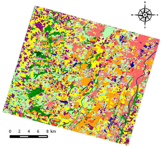
State-of-the-art approaches to producing accurate land cover maps use supervised classification of satellite images [3]. This makes it possible for maps to be reproducible and to be automatically produced at a global scale while reaching high levels of accuracy [4]. Figure 1 displays an example of such a map. Latest satellite constellations are capable of acquiring Satellite Image Time Series (SITS) with high spectral, spatial and temporal resolutions. For instance, the two Sentinel-2 satellites provide, since March 2017, worldwide images every five days, freely distributed, within 13 spectral bands at spatial resolutions varying from 10 to 60 m [5].
These new high-resolution SITS constitute an incredible source of data for land cover mapping, especially for vegetation and crop mapping [6,7], at regional and continental scales [4,8]. They also question the choice of the classification algorithms: although traditional algorithms showed good performance for SITS classification [3], they do not explicitly use the temporal relationship between acquisitions. Conversely, deep learning methods are appealing for this task [9], because they are capable of automatically extracting useful representations, as demonstrated both in the machine learning community [10] and in remote sensing [11]. The recent availability of long SITS on large areas calls for new studies to evaluate if (and how) SITS classification task can benefit from deep learning techniques.
In the following, we first review the state-of-the-art approaches used for SITS classification. Then, we describe the most recent applications of deep learning to remote sensing data, with focus on time series classification. Finally, we present the motivations and contributions of this work.
1.1. Traditional Approaches for SITS Classification
The state-of-the-art classification algorithms used to produce maps are currently Support Vector Machines (SVMs) and Random Forests (RFs) [12]. These algorithms are generally applied at pixel-level on the stack of multi-spectral images contained in the SITS. These algorithms are oblivious to the temporal dimension that structures SITS. The temporal order in which the images are presented has thus no influence on the results: counter-intuitively, a shuffle of the images in the series would result in the same model and thus in same accuracy. It induces a loss of the temporal behaviour for classes with evolution over time, such as the numerous forms of vegetation that are subject to seasonal change.
One solution to mitigate this problem has been to pre-calculate temporal features extracted from vegetation index time series, and then to feed them to a classification algorithm [13,14,15]. Temporal features that have been used include some statistical values, such as the maximum vegetation index, and the approximation of key dates in the phenological stages of the targeted vegetation classes, e.g., the time of peak vegetation index. However, the addition of such temporal features has shown little effect on classification performance [16].
To make the most of the temporal domain, other works have applied Nearest Neighbor (NN) -type approaches combined with temporal similarity measures [17]. Such measures aim at capturing the temporal trends present in the series by measuring a similarity independent of some temporal shifts between two time series [18]. Although promising, these methods require a complete scan of the training set for classifying each test instance—leading to prohibitive computational costs when using more than a few thousand profiles [19]—and only provide little abstraction of the training data.
1.2. Deep Learning in Remote Sensing
Deep learning approaches have been successfully used for many machine learning tasks including face detection [20], object recognition [21], and machine translation [22]. Benefiting from both theoretical and technical advances [23,24], they have shown to be extremely effective when there exists a relationship between the dimensions of the data such as for images, audio, or text. The applications to remote sensing of the two main deep learning architectures—Convolutional Neural Networks (CNNs) and Recurrent Neural Networks (RNNs)—are presented in the following.
1.2.1. Convolutional Neural Networks
CNNs have been widely applied to various remote sensing tasks including land cover classification of very high spatial resolution images [25,26], semantic segmentation [27], object detection [28], reconstruction of missing data [29], or pansharpening [30]. In these works, CNN models make the most of the spatial structure of the data by applying convolutions in both x and y dimensions. The main successful application of CNNs in remote sensing remains the classification of hyperspectral images, where 2D-CNNs across the spatial dimension have also been tested [31], as well as 1D-CNNs across the spectral dimension [32], and even 3D-CNNs across spectral and spatial dimensions [33,34].
Regarding the classification of multi-source and multi-temporal data, 1D-CNN and 2D-CNN have been used without taking advantage of the temporal dimension [35,36]: convolutions are applied either in the spectral domain or in the spatial domain, excluding the temporal one. In other words, the order of the images still has no influence on the model and results.
Meanwhile, temporal 1D-CNNs (TempCNNs) where convolutions are applied in the temporal domain have proven to be effective for handling the temporal dimension for (general) time series classification [37], and 3D-CNN for both the spatial and temporal dimension in video classification [38]. Consequently, these TempCNN architectures, that could make the most of the temporal structure of SITS have started to be explored in remote sensing where convolutions are applied across the temporal dimension alone [39,40], and also 3D-CNNs where convolutions are applied in both temporal and spatial dimensions [41]. In particular, these preliminary works highlight the potential of TempCNNs with higher accuracy than traditional algorithms such as RF. Although similar in nature with the work proposed in [40], this paper proposes an exhaustive study of TempCNNs (presented in Section 2) where we show how to handle multi-spectral images and use a broader nomenclature (not specific to summer crops).
1.2.2. Recurrent Neural Networks
RNNs are another type of deep learning architecture that are intrinsically designed for sequential data. For this reason, they have been the most studied architecture for SITS classification. They have demonstrated their potential for the classification of optical time series [42,43] as well as multi-temporal Synthetic Aperture Radar (SAR) [44,45]. Approaches have been tested with two types of units: Long-Short Term Memory (LSTM) and Gated Recurrent Units (GRUs) showing a small accuracy gain when using GRUs [42,46]. In addition, these works have shown that RNNs outperform traditional classification algorithms such as RFs or SVMs.
Some recent works dedicated to SITS classification have also combined RNNs with 2D-CNNs (spatial convolutions) either by merging representations learnt by the two types of networks [47] or by feeding a CNN model with the representation learned by a RNN model [48,49]. These types of combinations have also been used for land cover change detection task between multi-spectral images [50,51].
RNN models are able to explicitly consider the temporal correlation of the data [46] making them particularly well-suited to drawing a prediction at each time point, such as when translating each word in a sentence [22]. In remote sensing, an RNN model based on LSTM units has been proposed to output a land cover prediction at several time steps to detect palm oil plantations [52]. However, land cover mapping usually aims at producing one label for the whole series, where the label holds a temporal meaning (e.g., “corn crop”). RNNs might therefore be less suited to this specific classification task. In particular, the number of training steps (i.e., the number of back-propagation steps) is a function of the length of the series ([53] (Section 10.2.2)), while it is only a function of the depth of the network for CNNs. The result is a network that is: (1) harder to train because patterns at the start of the series are many layers away from the classification output, and (2) longer to train because the error has to be back-propagated through each layer in turn.
1.3. Our Contributions
In this paper, we extensively study the use of TempCNNs—where convolutions are applied in the temporal domain—for the classification of high-resolution SITS. The main contributions of this paper include:
- demonstrating the potential of TempCNNs against RFs and RNNs,
- showing the importance of temporal convolutions,
- evaluating the effect of additional hand-crafted spectral features such as vegetation indices,
- exploring the architecture of TempCNNs.
This paper proposes the study of TempCNN for SITS classification. We provide a methodological understanding of the models and their theoretical underpinnings, as well as an experimental study that gives general guidelines about how they should be used and parameterized. For this purpose, we first compare the classification performance of TempCNNs to the one of RFs and RNNs. Then, we discuss different architecture choices including size of the convolutions, pooling layers, width and depth of the network, regularization mechanisms and batch size. To our knowledge, this work is the first extensive study of TempCNNs for remote sensing to date. This paper focuses on 1D-CNN models and does not cover the use of the spatial structure of the data: each pixel is considered as an instance and the features learnt by the network are spectro-temporal. Similarly to previous studies, we work at pixel level and not at object level, mostly because the delineations of plots of land are not available for the whole studied area. Working at object level would thus require a pre-segmentation of the data that would introduce another dimension to this study and overly complicate the analysis. An interested reader could refer to [41] for a first exploration of that topic.
All the topics are addressed experimentally using 46 high-resolution Formosat-2 images, with training/test sets composed of one million labeled time series. This paper presents the results obtained over 2000 (79 architectures and 25 experiments for each) deep learning models. It corresponds to more than 2,000 hours of training time performed mainly on NVIDIA Tesla V100 Graphical Processing Units (GPUs).
This paper is organized as follows: Section 2 describes our TempCNN model which is used in the experiments. Then, Section 3 is dedicated to the description of the data and the experimental settings. Section 4 is the core section of the paper that presents our experimental results. Finally, Section 5 draws the main conclusions of this work.
2. Temporal Convolutional Neural Networks
This Section aims at presenting TempCNN models. We first briefly review the theory of neural networks and CNNs. We then present the principles of temporal convolutions. We finally introduce the general form of the TempCNN architecture studied in Section 4.
2.1. General Principles
Deep neural networks are based on the concatenation of different layers where each layer takes the outputs of the previous layer as inputs. Figure 2 shows an example of a fully-connected network where the neurons in green represent the input, the neurons in blue belong to the hidden layers and the neurons in red are the outputs. As depicted, each layer is composed of a certain number of units, also known as neurons. The input layer size depends on the dimension of the instances, whereas the output layer is composed of C units for a classification task with C classes. The number of hidden layers and their number of units need to be selected by the practitioner.
Formally, the outputs of a layer l, the activation maps denoted by , are obtained with a two-step calculation: it first takes a linear combination of the inputs—which are the output of layer , i.e., , and then it applies a non-linear activation function to this linear combination. It can be written as follow:
where and are the weights and the biases of the layer l, respectively, that need to be learned.
The activation function, denoted by in Equation (1), is crucial as it allows to introduce non-linear combinations of the features. If only linear functions were used, the depth of the network would have little effect since the final output would simply be a linear combination of the input, which could be achieved with a single layer. In this work, we use the well-kown Rectified Linear Units (ReLU), calculated as [23].
Stacking several layers allows to increase the capacity of the network to represent complex functions, while keeping the layers simple, i.e., composed of a small number of units. Section 4.4 will provide some experimental results for different network depths.
Let be a set of n training instances such as . The pair represents training instance i where is a D-variate time series of length T associated with the label for C classes. Formally, can be expressed by , where for a time stamp t. Note that is equal to in Equation (1).
Training a neural network corresponds to finding the values of and that will minimize a given cost function, which assesses the fit of the model to the data. This process is known as empirical risk minimization, and the cost function is usually defined as the average of the errors committed on each training instance:
where correspond to the network predictions.
The loss function , for a multi-class classification problem, is usually the cross-entropy loss:
where represents the probability of predicting the true class of instance i computed by the last layer of the network (the Softmax layer) and denoted for a network with L layers..
Training deep neural networks presents two main challenges which are offset by a substantial benefit. First, it requires significant expertise to engineer the architecture of the network, choose its hyper-parameters, and decide how to optimize it. In return, such models require less feature engineering than more traditional classification algorithms and have shown to provide superior accuracy across a wide range of tasks. It is in some sense shifting the difficulty linked to feature engineering to the one of architecture engineering. Second, deep neural networks are usually prone to overfitting because of their very low bias: they have so many parameters that they can fit a very large family of functions, which in turn creates an overfitting issue [54]. Section 4.4 will provide an analysis of TempCNN accuracy as a function of the number of learned parameters.
2.2. Temporal Convolutions
Convolutional layers were proposed to limit the number of weights that a network needs to learn while trying to make the most of the structuring dimensions in the data—e.g., spatial, temporal or spectral—[55]. They apply a convolution filter to the output of the previous layer. As compared to dense layers (i.e., the fully-connected layer presented in Section 2.1) where the output of a neuron is a single number reflecting the activation, the output of a convolution filter is an activation map. For example, if the input is a univariate time series, then the output will be a time series where each point in the series is the result of the convolution filter.
Figure 3 shows the application of a gradient extraction filter onto the time series depicted in blue. The output is depicted in red. It takes high positive values where an increase in the signal is detected, and low negative values where a decrease in the signal occurs. Note that the so-called convolution is technically a cross-correlation.
Convolutional layers have for specificity to share their parameters across different locations: the same linear combination is applied by sliding it over the entire input. This drastically reduces the number of weights in the layer, by assuming that the same convolution might be useful in different parts of the time series. This is why the number of trainable parameters only depends on the filter size of the convolution f and on the number of units n, but not on the size of the input. Conversely, the size of the output will depend on the size of the input, and also on two other hyper-parameters—the stride and the padding. The stride represents the interval between two convolution centers. Padding controls the addition of values (usually zeros) at the start and end of the input series, before the calculation of the convolution. It makes it possible, for instance, to ensure that the output has the same size as the input.
2.3. Proposed Network Architecture
In this section, we present the baseline architecture that will be discussed in this manuscript. Note that the goal of this paper is not to propose the best architecture for our data, but rather to explore the behaviour of TempCNNs for SITS classification through exhaustive experiments.
Figure 4 displays the base TempCNN architecture used in the experiments (Section 4). The architecture is composed of three convolutional layers (64 units), one dense layer (256 units) and one Softmax layer. The filter size of convolutions is set to 5. Section 4.4 will justify the width (i.e., number of units) and the depth (i.e., number of convolution layers) of this architecture. Moreover, Section 4.2 will study the influence of convolution filter size. Finally, the experimental section will also examine the use of pooling layers (Section 4.3).
To control for overfitting, we use four regularization mechanisms: dropout with a dropout rate of 0.5 [56], a -regularization on the weights (also named weight-decay) applied for all the layers with a small rate of , a validation set corresponding to 5% of the training set, and batch normalisation [24].
Similarly to the split between the train and test set (see the details in Section 3.2), the validation set is built such that instances do not come from the same polygons as ones from the train set. Section 4.5 will detail the influence of these four regularization mechanisms.
We train the network using Adam optimization (standard parameter values: , , and ) [57] with a batch size of 32, and a maximum number of epochs set to 20, with an early stopping mechanism with a patience of zero. The influence of the batch size on the accuracy and the training time are analysed in Section 4.6.
All the studied CNN models have been implemented with the Keras library [58], with Tensorflow as the backend [59]. To facilitate others to build on this work, we have made our code available at https://github.com/charlotte-pel/temporalCNN.
3. Material and Methods
This section presents the dataset used for the experiments. We first present the optical satellite data. Next, we briefly describe the reference data. Then, we detail the data preparation steps. Finally, we present the benchmark algorithms and evaluation measures.
3.1. Optical Satellite Data
The study area is located at the South West of France, near the city of Toulouse (1°10 E, 43°27 N). It is 24 km × 24 km area where about 60% of the soil correspond to arable surfaces. The area has a temperate continental climate with hot and dry summer—average temperature of about 22.4 °C and rainfall of about 38 mm per month. Figure 5 displays a satellite image of the area in false color from 14 July 2006.
The satellite dataset is composed of 46 Formosat-2 images acquired at 8 meter spatial resolution during the year 2006. Figure 6 shows the distribution of the acquisitions. Note that Formosat-2’s characteristics are similar to the new Sentinel-2 satellites that provide 10 m spatial resolution images every five days.
For each Formosat-2 image, only the three bands Near-Infrared (760–900 nm) (NIR), Red (630–690 nm) (R) and Green (520–600 nm) (G) are used. The blue channel has been discarded since it is sensitive to atmospheric artifacts.
Each image has been ortho-rectified to ensure the same pixel locations throughout the time series. In addition, the digital numbers from the row images have been converted to top-of-canopy reflectance by the French Space Agency [60]. This last step corrects images from atmospheric effects, and also outputs cloud, shadow and saturation masks. The remaining steps of the data preparation—temporal resampling, feature extraction and feature normalization—are presented in Section 3.3.
3.2. Reference Data
The reference data come from three sources: (1) farmer’s declaration from 2006 (Registre Parcellaire Graphique in French), (2) field campaigns performed during 2006, and (3) a reference map obtained with a semi-automatic procedure [61]. From these three reference sources, we extracted a total of 13 classes representing three winter crops (wheat, barley and rapeseed), five summer crops (e.g., corn, soy and sunflower), four natural classes (grassland, forests and water) and urban areas. Note that the reference map (3) is only used to extract the urban class, which is stable over time, and we checked the associated polygons visually.
Table 1 displays the total number of instances per class at pixel- and polygon-level. It shows great variations in the number of available instances for each class where grassland, urban surfaces, wheat and sunflower predominate.
The reference data are randomly split into two independent datasets at the polygon level where 60% of the data is used for training the classification algorithms and 40% is used for testing. To statistically evaluate the performance of the different algorithms, this splitting operation is repeated five times [62]. Hence, each algorithm is evaluated on five different train/test splits. To also take the variations from weights’ initialization into account, we train the neural networks five times on each train/test split. The presented results are then averaged over the 25 runs ().
3.3. Data Preparation
3.3.1. Temporal Resampling
The optical SITS includes invalid pixels due to the presence of clouds and saturated pixels. Nowadays, the high temporal resolution of SITS is used to efficiently detect clouds and their shadows [60]. The produced masks are then used to gap-fill the cloud-covered and saturated pixels before applying supervised classification algorithms, without a loss of accuracy [63]. We use here a temporal linear interpolation for imputing invalid pixel values. Although not perfect given the non-linear phenomena observed through the SITS, using more complex methods have shown only little impact on classification performance [64]. Note also that the biggest temporal gaps in the dataset occur mainly during the winter where the vegetation is not evolving much.
As most of the classification algorithms explored in the manuscript require a regular temporal sampling, we apply interpolation and resampling on a regular temporal grid defined with a time gap of two days. The starting and ending dates correspond to the first and last acquisition dates of the Formosat-2 series, respectively. This operation increases the length of the Formosat-2 time series from 46 to 149. As some studied algorithms, such as RF, may be sensitive to this increase of the length, we also keep the original temporal sampling with interpolation.
3.3.2. Feature Extraction
We calculate spectral indices after the gapfilling step for each element of the pixel series. Spectral indices are commonly used in addition of spectral bands as the input of the supervised classification system in the remote sensing literature [3]. They can help the classifier to handle some non-linear relationships between the spectral bands [4]
More specifically, we compute three commonly used indices: the Normalized Difference Vegetation Index (NDVI) [65], the Normalized Difference Water Index (NDWI) [66] and a brilliance index (IB) defined as the norm of all the available bands [63].
In the experiments, as we want to quantify the contribution of the spectral features on the different algorithms, we use a set of three different configurations: 1) NDVI only, 2) the spectral bands only (SB), and 3) the spectral bands and all indices (SB + NDVI + NDWI + IB). Note that we also decided to analyse NDVI separately, as it is the most common index for vegetation mapping. Table 2 summarizes the total number of variables for our SITS as a function of the temporal strategy and the spectral features that we use.
3.3.3. Feature Normalization
In remote sensing, the input time series are generally standardized by subtracting the mean and dividing by the standard deviation for each feature where each time stamp is considered as a separate feature. This standardization, named z-normalization of each band at each date in the following, ensures that the variation in the features is not dominated by a single feature that has a high dynamic rank. However, this transforms the general trend of the series.
In machine learning, the input data are generally z-normalized by subtracting the mean and divided by the standard deviation for each time series [67]. This z-normalization of each time series has been introduced to be able to compare time series that have similar trends, but different scaling and shifting [68]. However, it leads to a loss of the meaning of the magnitude, whereas magnitude is crucial for vegetation mapping, e.g., corn will have higher NDVI values than other summer crops.
To overcome both limitations of the common normalization methods, we use a min-max normalization per feature across all images. The traditional min-max normalization performs a subtraction of the minimum, then a division by the range, i.e., the maximum minus the minimum [69]. As this normalization is highly sensitive to extreme values, we propose to use 2% (or 98%) percentile rather than the minimum (or the maximum) value. For each feature, both percentile values are extracted from all the time-stamp values. In the following, this normalization is named global feature min/max normalization.
Figure 7 displays four NDVI temporal profiles (top left)—rapeseed, corn, deciduous and water—for the three types of normalization: z-normalization of each time series, z-normalization of each band at each date, global feature min/max normalization (2–98%). Z-normalization of each time series (top right) produces highly transformed temporal profiles, and loses the relative vertical positioning of the spectra. Similarly, z-normalization of each band at each date (bottom left) also modifies the meaning of the amplitude. For instance, the normalized rapeseed profile looks flat during the growing season (between day of year 35 and 75), although the NDVI increases during this period (indicating a growth of the plant). Finally, global feature min/max normalization (2–98%) (bottom right) is the only one that does not change the shape of the temporal profiles, while ensuring that most of the values are within .
3.4. Benchmark Algorithms
We use Random Forest (RF) as the state-of-the-art algorithm for SITS classification, and Recurrent Neural Networks (RNNs) as the leading deep learning algorithm for sequential data. Both benchmark algorithms are briefly introduced.
3.4.1. Random Forests
The remote sensing community has assessed the performance of different algorithms for SITS classification showing that Random Forest (RF) and Support Vector Machine (SVM) algorithms dominate other traditional algorithms [3,70]. In particular, the RF algorithm can handle the high dimension of the SITS data [16], is robust to the presence of mislabeled data [71], has high accuracy performance on large scale study [4], and has easy-to-tune parameters [16].
The RF algorithm builds an ensemble of binary decision trees [72]. Its first specificity is to use a bootstrap sample of the data at each tree—i.e., training instances are selected randomly with replacement [73]— in order to increase diversity among the trees. The second specificity is the use of random subspace technique for choosing the splitting criterion at each node: a subset of the features is first randomly selected, then all the possible splits on this subset are tested based on a feature value test, e.g., maximization of the Gini index. It results in a split of the data into two subsets, for which previous operations are recursively repeated. The construction stops when all the nodes are pure (i.e., in each node, all the instances belong to the same class), or when a user-defined criterion is met, such as a maximum depth or maximum number of instances at the node.
3.4.2. Recurrent Neural Networks
First developed for sequential data, RNN models have been recently applied to several classification tasks in remote sensing, and particularly for crop mapping [45,46,48]. They share the learnt features across different positions. As the error is back-propagated at each time step, the computational cost can be high and it might cause learning issues such as vanishing gradient. Hence, most recent RNN architectures use LSTM or GRU units that help to capture long distance connections and solve the vanishing gradient issue. They are composed of a memory cell as well as update and reset gates to decide how much new information to add and how much past information to forget. Moreover, RNNs are known to be able to handle series with different lengths, but to the best of our knowledge, not about dealing with an irregular sampling within one sequence.
Following the most recent studies, we train bidirectional RNNs with stacks of three GRUs, one dense layer with 256 neurons and a Softmax layer [46,48]. The same number of neurons is used in the three GRUs. More specifically, we have trained five different models comprised of 16, 32, 64, 128 or 256 neurons. As we focus on the analysis of TempCNNs in this paper, Section 4.1 will report only the best RNN result (128 neurons) obtained on the test instances. All the models have been trained similarly to the CNNs with Keras (backend Tensorflow): batch size equal to 32, Adam optimization, and monitoring of the validation loss with an early stopping mechanism (c.f., Section 2.3).
3.5. Performance Evaluation
We evaluate the performance of the different classification algorithms quantitatively and qualitatively. Following traditional quantitative evaluations, we calculate confusion matrices by comparing the reference labels with the predicted ones. Then, we compute the standard Overall Accuracy (OA) measure, as well as user’s accuracy (UA), producer’s accuracy (PA) and F-Score per-class. In addition, we also evaluate the results qualitatively through visual inspection.
4. Experimental Results
This section aims at evaluating the TempCNN architecture presented in Section 2.3. We designed a set of six experiments in order to study:
- how the proposed TempCNN architecture makes the most of both spectral and temporal dimensions,
- how the filter size of temporal convolutions influence the accuracy,
- how pooling layers influence the accuracy,
- how wide and deep the model should be,
- how the regularization mechanisms help training the model,
- what values should be used for batch size.
A last section is dedicated to the visual analysis of the produced land cover maps.
As explained in Section 3.2, all the presented Overall Accuracy (OA) values correspond to average values over five folds. When displayed, the interval always correspond to one standard deviation. All details of the trained networks are available at https://github.com/charlotte-pel/temporalCNN.
4.1. Benefiting from Both Spectral and Temporal Dimensions
In this experiment, we compare four configurations: (1) no guidance, (2) only temporal guidance, (3) only spectral guidance, and (4) both temporal and spectral guidance (TempCNNs). Before presenting the obtained results, we first describe the trained models for these fourth types of guidance, which are illustrated in Figure 8.
No guidance: Similar to a traditional classifier, such as the RF algorithm, the first considered type of model ignores the spectral and temporal structures of the data, i.e., the expected model is the same regardless of the order in which the features (spectral and temporal) are given. For this configuration, we decided to train two types of algorithms: (1) the RF classifier selected as the competitor [3], and (2) a deep learning model composed of three dense layers of 1024 units—this specific architecture is named FC in the following. Both models are trained the whole dataset with features, with T the length of the times series and D the number of spectral features (see Table 2). As both RF and FC models do not require regular temporal sampling, the use of 2-day sampling is not necessary and can even lead to under-performance. The use of high dimensional space composed of redundant and sometimes noisy features may indeed decrease accuracy. Hence, the results of both models are displayed for the original temporal sampling, i.e., .
Temporal guidance: The second type of model provides guidance only along the temporal dimension. We train an architecture with convolution filters of size . In other words, the same convolution filters are applied across the temporal dimension, identically for all the spectral dimensions (second column in Figure 8).
Spectral guidance: The third type of model includes guidance only on the spectral dimension (third column in Figure 8). For this purpose, a convolution of size is first applied without padding, reducing the spectral dimension to one for the next convolution layers of size .
Spectro-temporal guidance: The last type of model corresponds to the one presented in Section 2.3 (TempCNNs), where the first convolutions have size (last column in Figure 8). The choice of this architecture is explained in the following sections. We also compare this architecture to RNNs, which also provide a spectro-temporal guidance (Section 3.4).
It is interesting to note that studying temporal and spectral guidance separately is not standard; we only include it here as a means to disentangle the contribution of the different components of our TempCNN model. As illustrated by Figure 8, all the applied convolutions are 1D-convolutions as they slide over one dimension only: over time for both TempCNN and the temporal guidance, and the spectral dimension for the spectral guidance.
Table 3 displays the Overall Accuracy (OA) and one standard deviation for the four levels of guidance. As the use of engineering features may help the different models, we train all the models for the three types of features presented in Section 3.3: NDVI alone, spectral bands (SB), and spectral bands with three spectral indices (SB-SF). For both models using temporal guidance, the filter size f is set to five. All the models are learned as specified in Section 2.3, including dropout and batch normalization layers, weight decay and the use of a validation set.
Table 3 shows that the OA increases for CNN models when adding more guidance, regardless of the type of used features. Note that the case of only using the spectral guidance with NDVI feature is a particular “degenerate” case: the spectral dimension is composed of only one feature (NDVI). The trained model applies convolutions of size (1,1), leading to a model that does not provide any guidance.
When using at least the spectral bands in the feature vector (SB and SB-SF columns), our TempCNN model outperforms all other algorithms with variations in OA between 1 and 3%. We have also performed a paired t-test to compare the mean accuracy obtained over the different folds of TempCNNs against the three other competitors. The p-values are lower than for TempCNN vs both FC and RF, and for TempCNN vs RNN; TempCNN thus significantly outperforms the three models at the traditional 5% significance threshold.
Interestingly, models based on only spectral convolutions with spectral features (fifth row, second column) slightly outperform models that used only temporal guidance (fourth row, second column). This result confirms the importance of the spectral domain for land cover mapping application. In addition, the use of convolutions in both temporal and spectral domains leads to slightly better OA compared to the other three levels of guidance. Finally, Table 3 shows that the use of spectral indices in addition of the available spectral bands does not help to improve the accuracy of traditional and deep learning algorithms.
To explore this result further, Table 4 gives the producer’s accuracy (PA), the user’s accuracy (UA) and the F-Score per class for the three main classification algorithms: RFs, RNNs and TempCNNs.
Table 4 shows that TempCNNs outperform other algorithms with the highest F-Scores for all but two classes, while obtaining very close results for the two remaining classes. TempCNNs obtain very good results on the most frequent classes (wheat, sunflower, and grassland), but also on the rarer ones (peas, sorghum, and conifer).
4.2. Influence of the Filter Size
For CNN models using a temporal guidance, it is also interesting to study the filter size. Considering the 2-day regular temporal sampling, a filter size of f (with f an odd number) will abstract the temporal information over days, before and after each point of the series. Given this natural expression in number of days, we name the reach of the convolution: it corresponds to half of the width of the temporal neighborhood used for the temporal convolutions.
Table 5 displays the OA values as a function of reach for TempCNN. We study five size of filters corresponding to a reach of 2, 4, 8, 16, and 32 days, respectively.
Table 5 shows that the maximum OA is obtained for a reach of 8 days, with a similar OA for 4 days. The F-Score values per class corroborate this results where maxima are often achieved for a reach of 4 or 8 days. Although the OA values are close for the different reach values, there are some observable differences per class: conifer, sorgo, and pea have F-Score differences that range from 2.8 to 8.9%. This result shows the importance of the high temporal resolution SITS, such as the one provided at five days by both Sentinel-2 satellites. The frequency of acquisition indeed allows CNNs to abstract enough temporal information from the temporal convolutions. In general, the reach of the convolutions will mainly depend on the patterns that need to be abstracted at a given temporal resolution. For example, even though the F-scores are very similar w.r.t. reach, the conifer class seems to require the lowest reach and the deciduous to require the highest reach.
4.3. Are Local and Global Temporal Pooling Layers Important?
In this Section, we explore the use of pooling layers for different reach values. Pooling layers are generally used in image classification task to both speed-up the computations and make the learnt features more robust to noise [74]. They can be seen as a de-zooming operation, which naturally induces a multi-scale analysis when interleaved between successive convolutional layers. For a time series, these pooling layers simply reduce the length, and thus the resolution, of the time series that are output by the neurons—and this by a factor k.
Two types of pooling have received most of the attention in the literature in computer vision: 1) the local max-pooling [75], and 2) the global average pooling [76]. For time series, global average pooling seems to have been more successful [9,37]. We want to see here if these previous results can be generalized for time series classification.
For this purpose, we train models with a global average pooling layer added after the third convolution layers for the following reach: 2, 4, 8, 16, and 32 days. We also train models with local pooling layers interleaved between each convolution layer with a window size k of 2. As local pooling layers virtually increase the reach of the following convolutional layers for this experiment, we kept the reach constant—2, 4, 8, 16, and 32 days—by reducing the convolution filter size f after each convolution. For example, a constant reach of 8 is obtained by applying successively three convolutions with filter sizes of 9, 5, and 3, with a local pooling layer after each convolutional one.
Figure 9 displays the OA values as a function of reach. Each curve represents a different configuration: local max-pooling (MP) in blue, local max-pooling and global average pooling (MP + GAP) in orange, local average pooling (AP) in yellow, local and global average pooling (AP + GAP) in purple, and global average pooling (GAP) in green. The horizontal red dashed line corresponds to the OA values obtained without pooling layers in the previous experiment.
Figure 9 shows that the use of pooling layers performs poorly: the OA results are almost always below the one obtained without pooling layers (red dashed line). Let us describe in more details the different findings for both global and local pooling layers.
The use of a global average pooling layer leads to the biggest decrease in accuracy. This layer is generally used to drastically reduce the number of trainable parameters by reducing the size of the last convolution layer to its depth. It thus performs an extreme dimensionality reduction, that decreases here the accuracy performance.
Regarding the use of only local pooling layers, Figure 9 shows similar results for both max and average pooling layers. The OA values tend to decrease when the reach increases. The results are similar to those obtained by the model without pooling layers (horizontal red dashed line) for reach values lower than nine days, with even a slight improvement when using a local average pooling layer with a constant reach of four days.
This last result contrasts with results obtained in computer vision tasks for which: (1) max-pooling tends to give better results than average pooling, and (2) the use of local pooling layers helps to improve the classification performance. The main reason for this difference is probably task-related. In image classification, local pooling layers are known to extract features that are invariant to the scale and small transformations leading to models that can detect objects in an image no matter their locations or their sizes. However, the location of the temporal features, and their amplitude, are critical for SITS classification. For example, winter and summer crops, that we want to distinguish, may have similar profiles with only a shift in time. Removing the temporal location of the peak of greenness might prevent their discrimination.
4.4. How Wide and Deep a Model for Our Data?
4.4.1. Influence of the Width or Bias-Variance Trade-Off
This section has two goals: 1) justify the complexity of the learned models, and 2) be able to give an idea about how wide should the model be. Both objectives relate to the bias-variance trade-off of the model for our quantity of data. The more complex the model (i.e., more parameters), the lower its bias, i.e., the fewer incorrect assumptions the model makes about the distribution from which the data is sampled. Conversely, given a fixed quantity of training data, the more complex the model, the higher the variance. Many classifiers vary their bias-variance trade-offs automatically by changing their bias, such as decision trees tend to grow deeper as the quantity of data increases. For neural networks however, the bias is mostly fixed by the architecture, and the variance by the architecture and the quantity of training data. We use here the number of trainable parameters as a proxy for model complexity, which provides a reasonable measure when dealing with a specific classification problem where the quantity of data and the number of classes are fixed ([53] (Chapter 7, Introduction)).
We study seven CNN architectures with increasing number of parameters. Each architecture has three convolutional layers, one dense layer (256 neurons), and the Softmax layer as depicted in Figure 4. We then vary the number of neurons—or width—of the convolutional layers (16 to 1024 neurons). The depth of the model is specifically studied right after. The total number of trainable parameters then ranges from about 320,000 to 50 million. All models are trained following Section 2.3, with the exception of not using a validation set in order to observe more accuracy variations by letting the models being more prone to overfitting. Figure 10a shows the OA values as a function of number of parameters in logarithmic-scale.
Figure 10a shows that the architecture is very robust to a drastic change in number of parameters, as exhibited by OA varying only between 93.28% for 50M parameters and 93.69% for 2.5M parameters. The standard deviation increases with the number of parameters, but even at 50M parameters, most results are between 91% and 95% accuracy. Note that 50M parameters is an extremely large number of parameters for our dataset of about 620,000 training instances. From this result, one can see that models having about 2.5M of parameters with three convolutional layers and one dense layers have a good bias-variance trade-off.
If more training data is available, using a similar architecture is likely to conservatively work well, because more data is likely to drive the variance down while bias is fixed. If less data is available, one could decide to use a smaller architecture but again, overall, the results are very stable.
4.4.2. Influence of the Depth
We now propose here to vary the number of successive layers, i.e., the depth of the network, for the same model complexities. To keep the model complexity constant, we decrease the number of units for deeper networks. More specifically, we consider six architectures composed of one to six convolutional layers with a number of units ranging from 256 to 16, and one dense layer with a number of units ranging from 64 to 2048. Figure 10b shows OA values as a function of number of convolutions.
Figure 10b shows that the highest accuracies are obtained with the lowest standard deviation for an optimal number of convolutional layers of two or three. For a given complexity (here about 2.5M parameters), the use of an inappropriate number of convolutional layers and number of units may lead to an under-performance of TempCNNs. For a specific task, the selection of a reasonable architecture might be important, and could be optimized via cross-validation or using meta-learning approaches [77,78,79].
4.5. How to Control Overfitting?
Our TempCNN model includes four mechanisms to deal with overfitting: (1) regularization of the weights, (2) dropout, (3) using a validation set and (4) batch normalization. Regarding the optimal architecture in Section 4.4, the model needs to learn a number of parameters higher than more than three times the given number of training instances—2.5M of parameters versus 620,000 training data instances. This section aims at determining which of the used regularization mechanisms are the most important to train the TempCNN network. For this purpose, we first train our TempCNN architectures with only one regularization technique, then with all regularization techniques except one.
Table 6 displays OA values with or without the use of different regularization mechanisms. The first row displays the results when no regularization mechanism is applied (lower bound), whereas the last row displays the results when all the regularization mechanisms are used (higher bound).
Table 6 shows that the use of dropout is the most important regularization mechanism for TempCNNs as its only use leads to an OA value close from the one obtained when using the four regularization mechanisms. Conversely, the use of a validation set and the weight decay seem less useful to regularise the model.
4.6. What Values Should be Used for Batch Size?
This section aims at studying the influence of the batch size on the classification performance and on the training time. For this purpose, the model of Section 4.5 is trained for the following batch sizes: . Table 7 displays the OA values and also the training time for each studied batch size.
Table 7 shows that for our experiments the batch size influences the training time, but not the accuracy of the trained models, as all OA values are comparable. This result implies that large batch sizes can be selected to speed up training.
4.7. Visual Analysis
This experimental section ends with a visual analysis of the results for both blue and green areas of size 3.7 km × 3.6 km (465 pixels × 450 pixels) displayed in Figure 5. The analysis is performed for RF and TempCNN. The original temporal sampling is used for RF, whereas the regular temporal sampling at two days is used to train TempCNN. Both models are trained on the datasets with three spectral bands. The full maps are available in our online repository at https://github.com/charlotte-pel/temporalCNN.
Figure 11 displays the produced land cover maps. The first row displays the results for the blue area, whereas the second row displays the one for the green area. The first column displays the Formosat-2 image in false color for 14 July 2006 (zoom of Figure 6). The second and third columns give the results for the RF and the TempCNN algorithms, respectively. Images in the last column display the disagreements between both classifiers in red. Legend of land cover maps can be found in Table 1.
Although the results look visually similar, the disagreement images between both classifiers highlight some strong differences on the delineations between several land cover, but also at the object-level (e.g., crop, urban areas, forest). Regarding the delineation disagreements, we found that RF spreads out the majority class, i.e., urban areas, leading to an over-detection of this class, especially for mixing pixels. Regarding object disagreements, one can observe that RF mistakenly classifies an area as ‘urban’ (light pink) while it is a sunflower crop (purple). That crop, which was part of the test set, is highlighted with a green outline in the top-row results. Finally, this visual analysis shows that both classification algorithms exhibit some salt and pepper noise, that could be potentially removed by a post-processing procedure or by incorporating some spatial information into the classification framework.
5. Conclusions
This work explored the use of TempCNNs for SITS classification. Through an extensive set of experiments carried out on a series of 46 Formosat-2 images, we showed that the proposed TempCNN model outperforms RF and RNN algorithms by a margin of 1 to 3% in overall accuracy. A visual analysis also shows the good quality of TempCNN to accurately map land cover without over representation of majority classes.
To provide intuitions beyond this good performance, we studied the impact of the network architecture by varying the depth and the width of the models, by looking at the influence of common regularization mechanisms, and by exploring different batch size values. We have also demonstrated the importance of using both temporal and spectral dimensions when computing the convolutions. The remaining experimental results support two main recommendations on the use of pooling layers and the manual engineering of spectral features. First, we show that the use of global pooling layers, which drastically reduces the number of trainable parameters, is armful for SITS classification. Overall, we recommend careful study of the influence of pooling layers before any integration into a TempCNN network, and to favour local average pooling. Second, we show that the addition of manually-calculated spectral features, such as the NDVI, does not seem to improve TempCNN models. We thus recommend not to use them.
All these results show that TempCNNs are a very strong learner for Sentinel-2 SITS, which presents a high spectral resolution with 10 bands at a spatial resolution of 10 and 20 m. The presence of salt and pepper noise also indicates a need to take the spatial dimension of SITS into account, in addition to the spectral and temporal dimensions. Integrating the spatial dimension represents a good avenue for future research.
Author Contributions
All the authors have been involved in the writing of the manuscript and the design of experiments. C.P. has run the different experiments. Investigation, C.P.; Methodology, C.P., G.I.W. and F.P.; Writing—review & editing, C.P., G.I.W. and F.P.
Funding
François Petitjean is the recipient of an Australian Research Council Discovery Early Career Award (project number DE170100037) funded by the Australian Government. This material is based upon work supported by the Air Force Office of Scientific Research, Asian Office of Aerospace Research and Development (AOARD) under award number FA2386-18-1-4030.
Acknowledgments
The authors would like to thank their colleagues from the CESBIO laboratory (Jordi Inglada, Danielle Ducrot, Claire Marais-Sicre, Olivier Hagolle and Mireille Huc) for providing the reference land-cover maps as well as the corrected Formosat-2 images. They would also like to thank Hassan Ismail Fawaz and Germain Forestier for their comments on the manuscript, as well as anonymous reviewers for their very constructive comments.
Conflicts of Interest
The authors declare no conflict of interest.
Abbreviations
The following abbreviations are used in this manuscript:
| AP | Average Pooling |
| CNN | Convolutional Neural Network |
| GAP | Global Average Pooling |
| IB | Brilliance Index |
| MP | Max pooling |
| NDVI | Normalized Difference Vegetation Index |
| NDWI | Normalized Difference Water Index |
| OA | Overall Accuracy |
| RF | Random Forests |
| RNN | Recurrent Neural Network |
| SB | Spectral Band |
| SITS | Satellite Image Time Series |
| SVM | Support Vector machine |
| TempCNN | Temporal Convolutional Neural Network |
References
- Bojinski, S.; Verstraete, M.; Peterson, T.C.; Richter, C.; Simmons, A.; Zemp, M. The concept of essential climate variables in support of climate research, applications, and policy. Bull. Am. Meteorol. Soc. 2014, 95, 1431–1443. [Google Scholar] [CrossRef]
- Feddema, J.J.; Oleson, K.W.; Bonan, G.B.; Mearns, L.O.; Buja, L.E.; Meehl, G.A.; Washington, W.M. The importance of land-cover change in simulating future climates. Science 2005, 310, 1674–1678. [Google Scholar] [CrossRef] [PubMed]
- Gómez, C.; White, J.C.; Wulder, M.A. Optical remotely sensed time series data for land cover classification: A review. ISPRS J. Photogramm. Remote Sens. 2016, 116, 55–72. [Google Scholar] [CrossRef] [Green Version]
- Inglada, J.; Vincent, A.; Arias, M.; Tardy, B.; Morin, D.; Rodes, I. Operational high resolution land cover map production at the country scale using satellite image time series. Remote Sens. 2017, 9, 95. [Google Scholar] [CrossRef]
- Drusch, M.; Del Bello, U.; Carlier, S.; Colin, O.; Fernandez, V.; Gascon, F.; Hoersch, B.; Isola, C.; Laberinti, P.; Martimort, P.; et al. Sentinel-2: ESA’s Optical High-Resolution Mission for GMES Operational Services. Remote Sens. Environ. 2012, 120, 25–36. [Google Scholar] [CrossRef]
- Matton, N.; Sepulcre, G.; Waldner, F.; Valero, S.; Morin, D.; Inglada, J.; Arias, M.; Bontemps, S.; Koetz, B.; Defourny, P. An automated method for annual cropland mapping along the season for various globally-distributed agrosystems using high spatial and temporal resolution time series. Remote Sens. 2015, 7, 13208–13232. [Google Scholar] [CrossRef]
- Vuolo, F.; Neuwirth, M.; Immitzer, M.; Atzberger, C.; Ng, W.T. How much does multi-temporal Sentinel-2 data improve crop type classification? Int. J. Appl. Earth Obs. Geoinf. 2018, 72, 122–130. [Google Scholar] [CrossRef]
- Immitzer, M.; Vuolo, F.; Atzberger, C. First experience with Sentinel-2 data for crop and tree species classifications in central Europe. Remote Sens. 2016, 8, 166. [Google Scholar] [CrossRef]
- Ismail Fawaz, H.; Forestier, G.; Weber, J.; Idoumghar, L.; Muller, P.A. Deep learning for time series classification: A review. arXiv, 2018; arXiv:1809.04356. [Google Scholar]
- Bengio, Y.; Courville, A.; Vincent, P. Representation learning: A review and new perspectives. IEEE Trans. Pattern Anal. Mach. Intell. 2013, 35, 1798–1828. [Google Scholar] [CrossRef] [PubMed]
- Zhu, X.X.; Tuia, D.; Mou, L.; Xia, G.S.; Zhang, L.; Xu, F.; Fraundorfer, F. Deep Learning in Remote Sensing: A Comprehensive Review and List of Resources. IEEE Geosci. Remote Sens. Mag. 2017, 5, 8–36. [Google Scholar] [CrossRef] [Green Version]
- Khatami, R.; Mountrakis, G.; Stehman, S.V. A meta-analysis of remote sensing research on supervised pixel-based land-cover image classification processes: General guidelines for practitioners and future research. Remote Sens. Environ. 2016, 177, 89–100. [Google Scholar] [CrossRef] [Green Version]
- Jia, K.; Liang, S.; Wei, X.; Yao, Y.; Su, Y.; Jiang, B.; Wang, X. Land cover classification of Landsat data with phenological features extracted from time series MODIS NDVI data. Remote Sens. 2014, 6, 11518–11532. [Google Scholar] [CrossRef]
- Pittman, K.; Hansen, M.C.; Becker-Reshef, I.; Potapov, P.V.; Justice, C.O. Estimating global cropland extent with multi-year MODIS data. Remote Sens. 2010, 2, 1844–1863. [Google Scholar] [CrossRef]
- Valero, S.; Morin, D.; Inglada, J.; Sepulcre, G.; Arias, M.; Hagolle, O.; Dedieu, G.; Bontemps, S.; Defourny, P.; Koetz, B. Production of a dynamic cropland mask by processing remote sensing image series at high temporal and spatial resolutions. Remote Sens. 2016, 8, 55. [Google Scholar] [CrossRef]
- Pelletier, C.; Valero, S.; Inglada, J.; Champion, N.; Dedieu, G. Assessing the robustness of Random Forests to map land cover with high resolution satellite image time series over large areas. Remote Sens. Environ. 2016, 187, 156–168. [Google Scholar] [CrossRef]
- Petitjean, F.; Inglada, J.; Gançarski, P. Satellite image time series analysis under time warping. IEEE Trans. Geosci. Remote Sens. 2012, 50, 3081–3095. [Google Scholar] [CrossRef]
- Maus, V.; Câmara, G.; Cartaxo, R.; Sanchez, A.; Ramos, F.M.; de Queiroz, G.R. A time-weighted dynamic time warping method for land-use and land-cover mapping. IEEE J. Sel. Top. Appl. Earth Obs. Remote Sens. 2016, 9, 3729–3739. [Google Scholar] [CrossRef]
- Belgiu, M.; Csillik, O. Sentinel-2 cropland mapping using pixel-based and object-based time-weighted dynamic time warping analysis. Remote Sens. Environ. 2018, 204, 509–523. [Google Scholar] [CrossRef]
- Schroff, F.; Kalenichenko, D.; Philbin, J. Facenet: A unified embedding for face recognition and clustering. In Proceedings of the IEEE Conference on Computer Vision and Pattern Recognition, Boston, MA, USA, 7–12 June 2015; pp. 815–823. [Google Scholar]
- Redmon, J.; Farhadi, A. YOLO9000: Better, Faster, Stronger. In Proceedings of the 2017 IEEE Conference on Computer Vision and Pattern Recognition (CVPR), Honolulu, HI, USA, 21–26 July 2017; pp. 6517–6525. [Google Scholar]
- Bahdanau, D.; Cho, K.; Bengio, Y. Neural machine translation by jointly learning to align and translate. In Proceedings of the International Conference on Learning Representations (ICLR), Banff, AB, Canada, 14–16 April 2014. [Google Scholar]
- Krizhevsky, A.; Sutskever, I.; Hinton, G.E. Imagenet classification with deep convolutional neural networks. In Proceedings of the 25th International Conference on Neural Information Processing Systems, Lake Tahoe, NV, USA, 3–8 December 2012; pp. 1097–1105. [Google Scholar]
- Ioffe, S.; Szegedy, C. Batch Normalization: Accelerating Deep Network Training by Reducing Internal Covariate Shift. In Proceedings of the International Conference on Machine Learning, Lille, France, 6–11 July 2015; pp. 448–456. [Google Scholar]
- Maggiori, E.; Tarabalka, Y.; Charpiat, G.; Alliez, P. Convolutional Neural Networks for large-scale remote-sensing image classification. IEEE Trans. Geosci. Remote Sens. 2017, 55, 645–657. [Google Scholar] [CrossRef]
- Postadjian, T.; Le Bris, A.; Sahbi, H.; Mallet, C. Investigating the potential of deep neural networks for large-scale classification of very high resolution satellite images. ISPRS Ann. Photogramm. Remote Sens. Spat. Inf. Sci. 2017, 4, 183–190. [Google Scholar] [CrossRef]
- Volpi, M.; Tuia, D. Dense semantic labeling of subdecimeter resolution images with convolutional neural networks. IEEE Trans. Geosci. Remote Sens. 2017, 55, 881–893. [Google Scholar] [CrossRef]
- Audebert, N.; Le Saux, B.; Lefèvre, S. Segment-before-detect: Vehicle detection and classification through semantic segmentation of aerial images. Remote Sens. 2017, 9, 368. [Google Scholar] [CrossRef]
- Zhang, Q.; Yuan, Q.; Zeng, C.; Li, X.; Wei, Y. Missing Data Reconstruction in Remote Sensing image with a Unified Spatial-Temporal-Spectral Deep Convolutional Neural Network. IEEE Trans. Geosci. Remote Sens. 2018, 56, 4274–4288. [Google Scholar] [CrossRef]
- Masi, G.; Cozzolino, D.; Verdoliva, L.; Scarpa, G. Pansharpening by Convolutional Neural Networks. Remote Sens. 2016, 8, 594. [Google Scholar] [CrossRef]
- Liang, H.; Li, Q. Hyperspectral imagery classification using sparse representations of convolutional neural network features. Remote Sens. 2016, 8, 99. [Google Scholar] [CrossRef]
- Hu, F.; Xia, G.S.; Hu, J.; Zhang, L. Transferring deep convolutional neural networks for the scene classification of high-resolution remote sensing imagery. Remote Sens. 2015, 7, 14680–14707. [Google Scholar] [CrossRef]
- Li, Y.; Zhang, H.; Shen, Q. Spectral–spatial classification of hyperspectral imagery with 3D convolutional neural network. Remote Sens. 2017, 9, 67. [Google Scholar] [CrossRef]
- Hamida, A.B.; Benoit, A.; Lambert, P.; Amar, C.B. 3-D Deep Learning Approach for Remote Sensing Image Classification. IEEE Trans. Geosci. Remote Sens. 2018, 56, 4420–4434. [Google Scholar] [CrossRef]
- Kussul, N.; Lavreniuk, M.; Skakun, S.; Shelestov, A. Deep learning classification of land cover and crop types using remote sensing data. IEEE Geosci. Remote Sens. Lett. 2017, 14, 778–782. [Google Scholar] [CrossRef]
- Scarpa, G.; Gargiulo, M.; Mazza, A.; Gaetano, R. A CNN-Based Fusion Method for Feature Extraction from Sentinel Data. Remote Sens. 2018, 10, 236. [Google Scholar] [CrossRef]
- Wang, Z.; Yan, W.; Oates, T. Time series classification from scratch with deep neural networks: A strong baseline. In Proceedings of the International Joint Conference on Neural Networks (IJCNN), Anchorage, AK, USA, 14–19 May 2017; pp. 1578–1585. [Google Scholar]
- Wu, Z.; Wang, X.; Jiang, Y.G.; Ye, H.; Xue, X. Modeling spatial-temporal clues in a hybrid deep learning framework for video classification. In Proceedings of the 23rd ACM International Conference on Multimedia, Brisbane, Australia, 26–30 October 2015; pp. 461–470. [Google Scholar]
- Di Mauro, N.; Vergari, A.; Basile, T.M.A.; Ventola, F.G.; Esposito, F. End-to-end Learning of Deep Spatio-temporal Representations for Satellite Image Time Series Classification. In Proceedings of the European Conference on Machine Learning & Principles and Practice of Knowledge Discovery in Databases (PKDD/ECML), Skopje, Macedonia, 18–22 September 2017. [Google Scholar]
- Zhong, L.; Hu, L.; Zhou, H. Deep learning based multi-temporal crop classification. Remote Sens. Environ. 2019, 221, 430–443. [Google Scholar] [CrossRef]
- Ji, S.; Zhang, C.; Xu, A.; Shi, Y.; Duan, Y. 3D Convolutional Neural Networks for Crop Classification with Multi-Temporal Remote Sensing Images. Remote Sens. 2018, 10, 75. [Google Scholar] [CrossRef]
- RuBwurm, M.; Körner, M. Temporal Vegetation Modelling Using Long Short-Term Memory Networks for Crop Identification from Medium-Resolution Multi-spectral Satellite Images. In Proceedings of the Computer Vision and Pattern Recognition Workshops, Honolulu, HI, USA, 21–26 July 2017; pp. 1496–1504. [Google Scholar]
- Sun, Z.; Di, L.; Fang, H. Using Long Short-Term Memory Recurrent Neural Network in land cover classification on Landsat and Cropland data layer time series. Int. J. Remote Sens. 2018, 40, 1–22. [Google Scholar] [CrossRef]
- Ienco, D.; Gaetano, R.; Dupaquier, C.; Maurel, P. Land Cover Classification via Multitemporal Spatial Data by Deep Recurrent Neural Networks. IEEE Geosci. Remote Sens. Lett. 2017, 14, 1685–1689. [Google Scholar] [CrossRef] [Green Version]
- Minh, D.H.T.; Ienco, D.; Gaetano, R.; Lalande, N.; Ndikumana, E.; Osman, F.; Maurel, P. Deep recurrent neural networks for winter vegetation quality mapping via multitemporal SAR Sentinel-1. IEEE Geosci. Remote Sens. Lett. 2018, 15, 464–468. [Google Scholar] [CrossRef]
- Ndikumana, E.; Ho Tong Minh, D.; Baghdadi, N.; Courault, D.; Hossard, L. Deep Recurrent Neural Network for Agricultural Classification using multitemporal SAR Sentinel-1 for Camargue, France. Remote Sens. 2018, 10, 1217. [Google Scholar] [CrossRef]
- Benedetti, P.; Ienco, D.; Gaetano, R.; Ose, K.; Pensa, R.G.; Dupuy, S. M3-Fusion: A Deep Learning Architecture for Multiscale Multimodal Multitemporal Satellite Data Fusion. IEEE J. Sel. Top. Appl. Earth Obs. Remote Sens. 2018, 11, 4939–4949. [Google Scholar] [CrossRef]
- Rußwurm, M.; Körner, M. Multi-temporal land cover classification with sequential recurrent encoders. ISPRS Int. J. Geo-Inf. 2018, 7, 129. [Google Scholar] [CrossRef]
- Rußwurm, M.; Körner, M. Convolutional LSTMs for Cloud-Robust Segmentation of Remote Sensing Imagery. In Proceedings of the Spatio-Temporal Workshop on Neural Information Processing Systems, Montreal, QC, Canada, 3–8 December 2018. [Google Scholar]
- Lyu, H.; Lu, H.; Mou, L. Learning a transferable change rule from a recurrent neural network for land cover change detection. Remote Sens. 2016, 8, 506. [Google Scholar] [CrossRef]
- Mou, L.; Bruzzone, L.; Zhu, X.X. Learning spectral-spatial-temporal features via a recurrent convolutional neural network for change detection in multispectral imagery. IEEE Trans. Geosci. Remote Sens. 2019, 57, 924–935. [Google Scholar] [CrossRef]
- Jia, X.; Khandelwal, A.; Nayak, G.; Gerber, J.; Carlson, K.; West, P.; Kumar, V. Incremental dual-memory LSTM in land cover prediction. In Proceedings of the 23rd ACM SIGKDD International Conference on Knowledge Discovery and Data Mining, Halifax, NS, Canada, 13–17 August 2017; pp. 867–876. [Google Scholar]
- Goodfellow, I.; Bengio, Y.; Courville, A. Deep Learning; MIT Press: Cambridge, MA, USA, 2016. [Google Scholar]
- Zhang, C.; Bengio, S.; Hardt, M.; Recht, B.; Vinyals, O. Understanding deep learning requires rethinking generalization. In Proceedings of the International Conference on Learning Representations (ICLR), Toulon, France, 24–26 April 2017. [Google Scholar]
- LeCun, Y.; Boser, B.E.; Denker, J.S.; Henderson, D.; Howard, R.E.; Hubbard, W.E.; Jackel, L.D. Handwritten digit recognition with a back-propagation network. In Advances in Neural Information Processing Systems; Morgan Kaufmann Publishers Inc.: San Francisco, CA, USA, 1990; pp. 396–404. [Google Scholar]
- Srivastava, N.; Hinton, G.; Krizhevsky, A.; Sutskever, I.; Salakhutdinov, R. Dropout: A simple way to prevent neural networks from overfitting. J. Mach. Learn. Res. 2014, 15, 1929–1958. [Google Scholar]
- Kingma, D.P.; Ba, J. Adam: A method for stochastic optimization. In Proceedings of the International Conference on Learning Representations (ICLR), Banff, AB, Canada, 14–16 April 2014. [Google Scholar]
- Chollet, F. Keras. 2015. Available online: https://keras.io (accessed on 1 February 2018).
- Abadi, M.; Barham, P.; Chen, J.; Chen, Z.; Davis, A.; Dean, J.; Devin, M.; Ghemawat, S.; Irving, G.; Isard, M.; et al. TensorFlow: A System for Large-Scale Machine Learning. In Proceedings of the 12th USENIX Symposium on Operating Systems Design and Implementation, OSDI 2016, Savannah, GA, USA, 2–4 November 2016; Volume 16, pp. 265–283. [Google Scholar]
- Hagolle, O.; Huc, M.; Villa Pascual, D.; Dedieu, G. A multi-temporal and multi-spectral method to estimate aerosol optical thickness over land, for the atmospheric correction of FormoSat-2, LandSat, VENUS and Sentinel-2 images. Remote Sens. 2015, 7, 2668–2691. [Google Scholar] [CrossRef]
- Idbraim, S.; Ducrot, D.; Mammass, D.; Aboutajdine, D. An unsupervised classification using a novel ICM method with constraints for land cover mapping from remote sensing imagery. Int. Rev. Comput. Softw. 2009, 4, 165–176. [Google Scholar]
- Lyons, M.B.; Keith, D.A.; Phinn, S.R.; Mason, T.J.; Elith, J. A comparison of resampling methods for remote sensing classification and accuracy assessment. Remote Sens. Environ. 2018, 208, 145–153. [Google Scholar] [CrossRef]
- Inglada, J.; Arias, M.; Tardy, B.; Hagolle, O.; Valero, S.; Morin, D.; Dedieu, G.; Sepulcre, G.; Bontemps, S.; Defourny, P.; et al. Assessment of an operational system for crop type map production using high temporal and spatial resolution satellite optical imagery. Remote Sens. 2015, 7, 12356–12379. [Google Scholar] [CrossRef]
- Valero, S.; Pelletier, C.; Bertolino, M. Patch-based reconstruction of high resolution satellite image time series with missing values using spatial, spectral and temporal similarities. In Proceedings of the IEEE International Geoscience and Remote Sensing Symposium (IGARSS), Beijing, China, 10–15 July 2016; pp. 2308–2311. [Google Scholar]
- Rouse, J., Jr.; Haas, R.; Schell, J.; Deering, D. Monitoring vegetation systems in the Great Plains with ERTS. In Proceedings of the Third Symposium on Significant Results Obtained from the First Earth, Washington, DC, USA, 10–14 December 1973. [Google Scholar]
- McFeeters, S.K. The use of the Normalized Difference Water Index (NDWI) in the delineation of open water features. Int. J. Remote Sens. 1996, 17, 1425–1432. [Google Scholar] [CrossRef]
- Bagnall, A.; Lines, J.; Bostrom, A.; Large, J.; Keogh, E. The great time series classification bake off: A review and experimental evaluation of recent algorithmic advances. Data Min. Knowl. Discov. 2017, 31, 606–660. [Google Scholar] [CrossRef]
- Goldin, D.Q.; Kanellakis, P.C. On similarity queries for time-series data: Constraint specification and implementation. In International Conference on Principles and Practice of Constraint Programming; Springer: Cassis, France, 1995; pp. 137–153. [Google Scholar]
- Han, J.; Pei, J.; Kamber, M. Data Mining: Concepts and Techniques; Elsevier: Amsterdam, The Netherlands, 2011. [Google Scholar]
- Belgiu, M.; Drăguţ, L. Random Forest in remote sensing: A review of applications and future directions. ISPRS J. Photogramm. Remote Sens. 2016, 114, 24–31. [Google Scholar] [CrossRef]
- Pelletier, C.; Valero, S.; Inglada, J.; Champion, N.; Marais Sicre, C.; Dedieu, G. Effect of training class label noise on classification performances for land cover mapping with satellite image time series. Remote Sens. 2017, 9, 173. [Google Scholar] [CrossRef]
- Breiman, L. Random Forests. Mach. Learn. 2001, 45, 5–32. [Google Scholar] [CrossRef] [Green Version]
- Breiman, L. Bagging predictors. Mach. Learn. 1996, 24, 123–140. [Google Scholar] [CrossRef] [Green Version]
- Boureau, Y.L.; Ponce, J.; LeCun, Y. A theoretical analysis of feature pooling in visual recognition. In Proceedings of the 27th International Conference on Machine Learning (ICML-10), Haifa, Israel, 21–24 June 2010; pp. 111–118. [Google Scholar]
- Ren, S.; He, K.; Girshick, R.; Sun, J. Faster r-CNN: Towards real-time object detection with region proposal networks. In Proceedings of the Advances in Neural Information Processing Systems, Montreal, QC, Canada, 7–12 December 2015; pp. 91–99. [Google Scholar]
- He, K.; Zhang, X.; Ren, S.; Sun, J. Deep residual learning for image recognition. In Proceedings of the IEEE Conference on Computer Vision and Pattern Recognition, Las Vegas, Nevada, USA, 27–30 June 2016; pp. 770–778. [Google Scholar]
- Bergstra, J.; Bengio, Y. Random search for hyper-parameter optimization. J. Mach. Learn. Res. 2012, 13, 281–305. [Google Scholar]
- Hutter, F.; Hoos, H.H.; Leyton-Brown, K. Sequential model-based optimization for general algorithm configuration. In Proceedings of the International Conference on Learning and Intelligent Optimization, Rome, Italy, 17–21 January 2011; pp. 507–523. [Google Scholar]
- Snoek, J.; Larochelle, H.; Adams, R.P. Practical bayesian optimization of machine learning algorithms. In Proceedings of the Advances in Neural Information Processing Systems, Lake Tahoe, NV, USA, 3–8 December 2012; pp. 2951–2959. [Google Scholar]
Figure 1.
An example land cover map.

Figure 2.
Example of fully-connected neural network.

Figure 3.
Convolution of a time series (blue) with the positive gradient filter (black). The result (red) takes high positive values when the signal sharply increases, and conversely.
Figure 3.
Convolution of a time series (blue) with the positive gradient filter (black). The result (red) takes high positive values when the signal sharply increases, and conversely.

Figure 4.
Proposed temporal Convolutional Neural Network (TempCNN). The network input is a multi-variate time series. Three convolutional filters are consecutively applied, then one dense layer, and finally the Softmax layer, that provides the predicting class distribution.
Figure 4.
Proposed temporal Convolutional Neural Network (TempCNN). The network input is a multi-variate time series. Three convolutional filters are consecutively applied, then one dense layer, and finally the Softmax layer, that provides the predicting class distribution.

Figure 5.
Formosat-2 image in false color (near infra-red, red, green) from 14 July 2006. Green and blue squares will be inspected visually in the experiments.
Figure 5.
Formosat-2 image in false color (near infra-red, red, green) from 14 July 2006. Green and blue squares will be inspected visually in the experiments.

Figure 6.
Acquisition dates of the Formosat-2 image time series.

Figure 7.
Three types of normalization of four Normalized Difference Vegetation Index (NDVI) temporal profiles.
Figure 7.
Three types of normalization of four Normalized Difference Vegetation Index (NDVI) temporal profiles.

Figure 8.
Types of guidance. The top row represents our input in a 2D array, whereas the bottom row represents the output of one neuron under each guidance scheme.
Figure 8.
Types of guidance. The top row represents our input in a 2D array, whereas the bottom row represents the output of one neuron under each guidance scheme.

Figure 9.
Overall Accuracy (OA) as function of reach for local max-pooling (MP) in blue, local max-pooling and global average pooling (MP + GAP) in orange, local average pooling (AP) in yellow, local and global average pooling (AP + GAP) in purple, and global average pooling (GAP) alone in green. We use the dataset with three spectral bands and a regular temporal sampling at two days.

Figure 10.
Overall Accuracy (±one standard deviation in orange) as a function of the number of parameters (a) or the number of successive convolutional layers (b) for seven temporal Convolutional Neural Network models. We use the dataset with three spectral bands and a regular temporal sampling at two days.

Figure 11.
Visual results for two areas. The first column displays the Formosat-2 image in false color from 14 July 2006. The second and third columns give the results for Random Forest (RF) and our TempCNN model, respectively. The images in the last column displays in red the disagreement between both classifiers. Legend of land cover maps is given in Table 1.


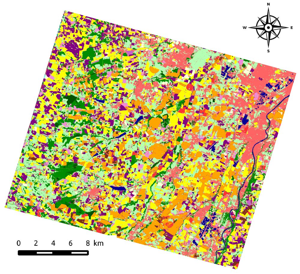
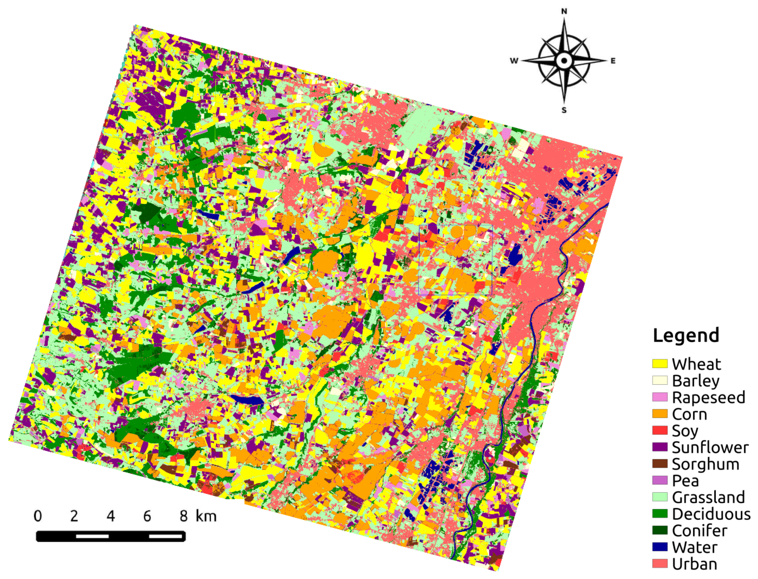
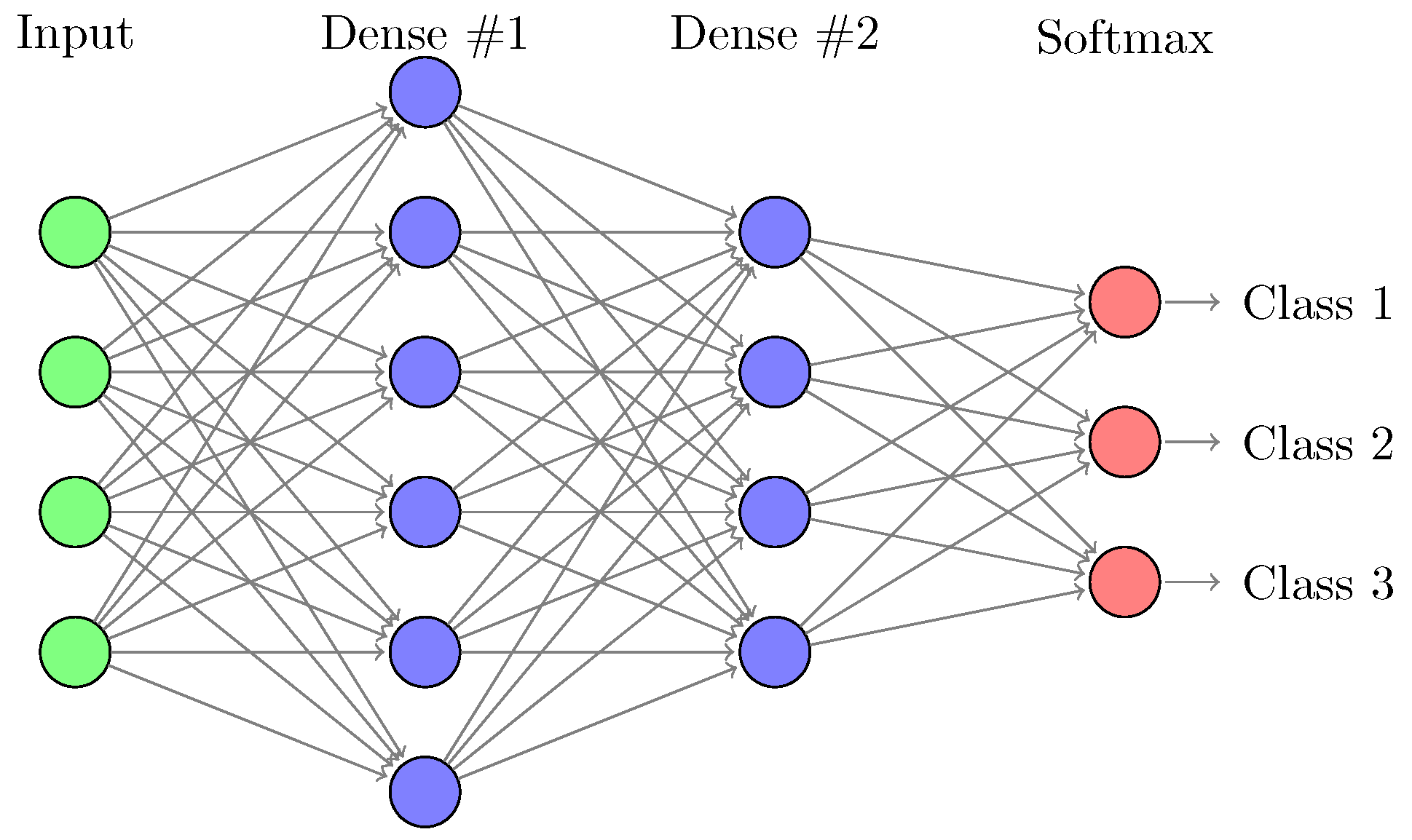
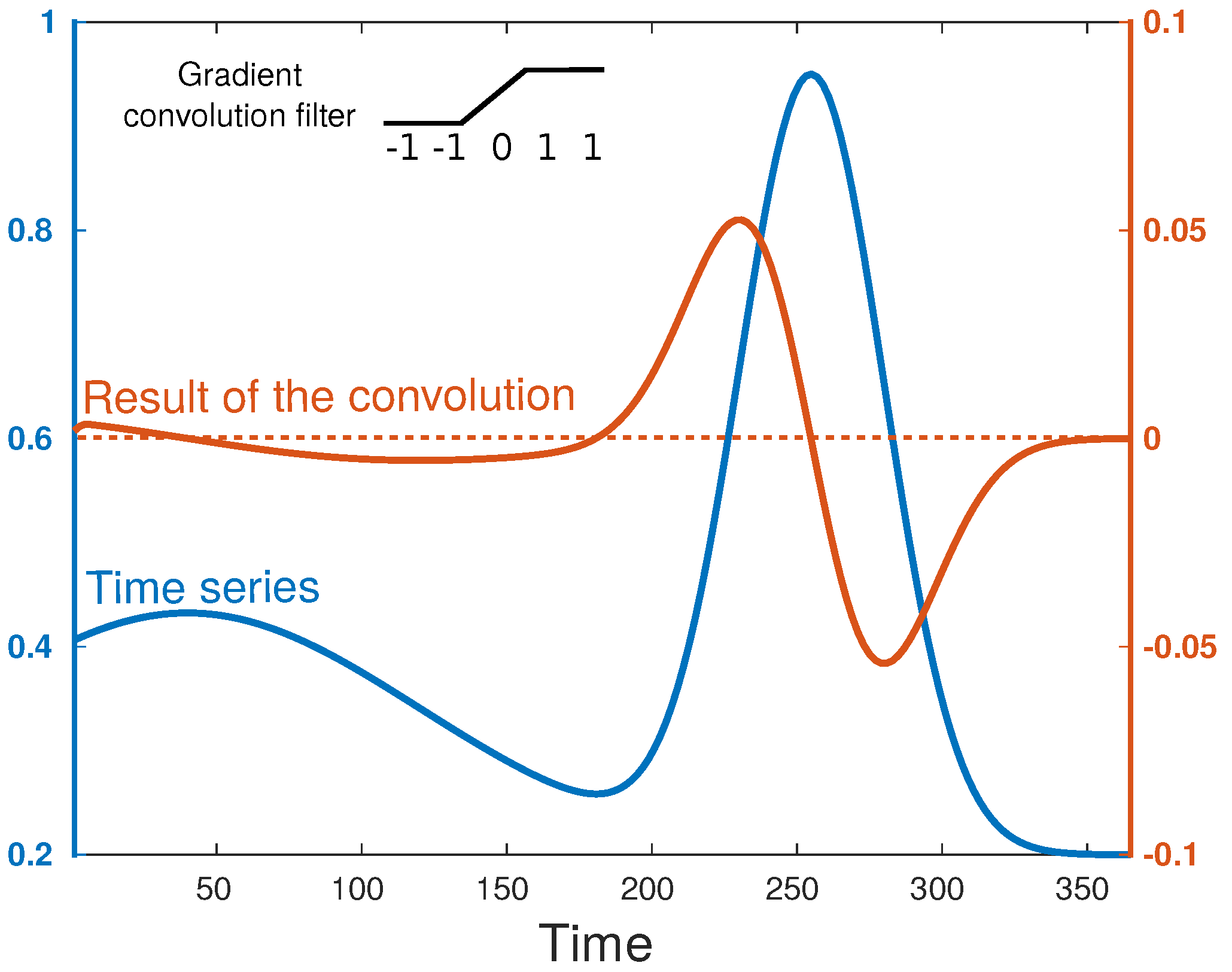
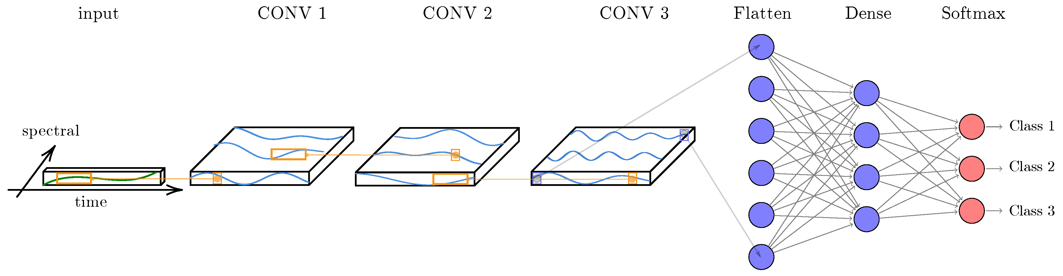
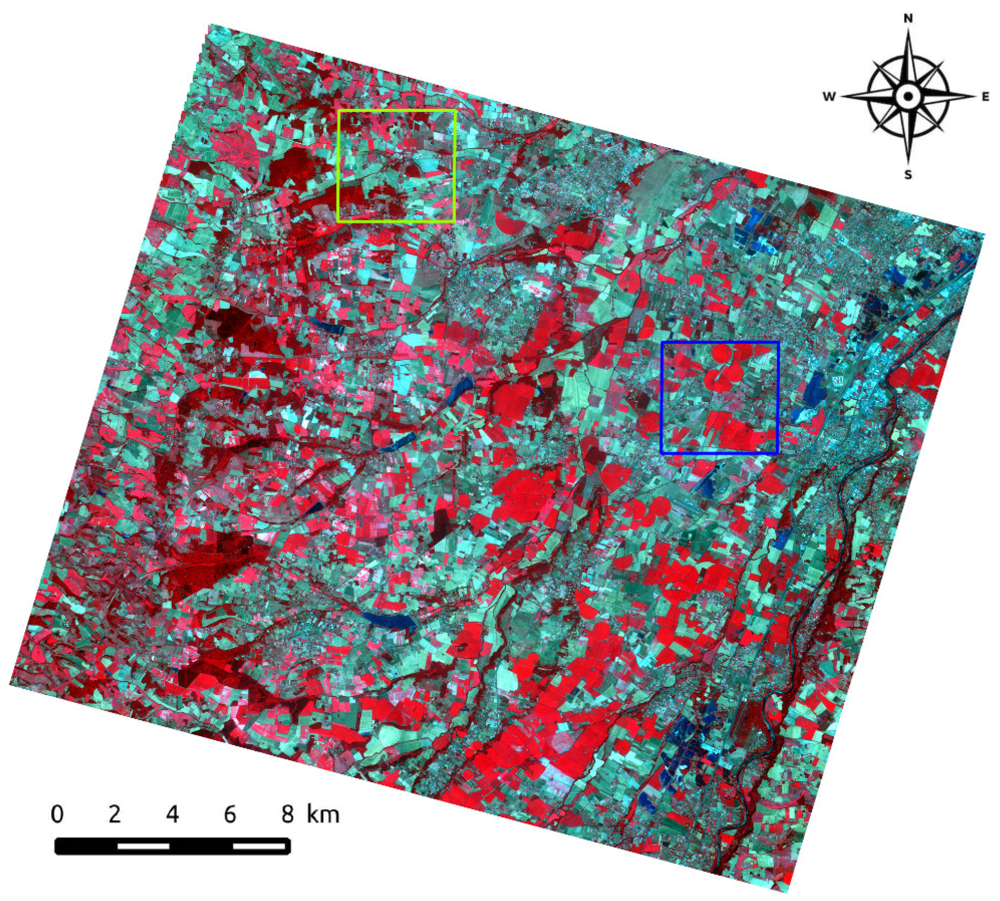
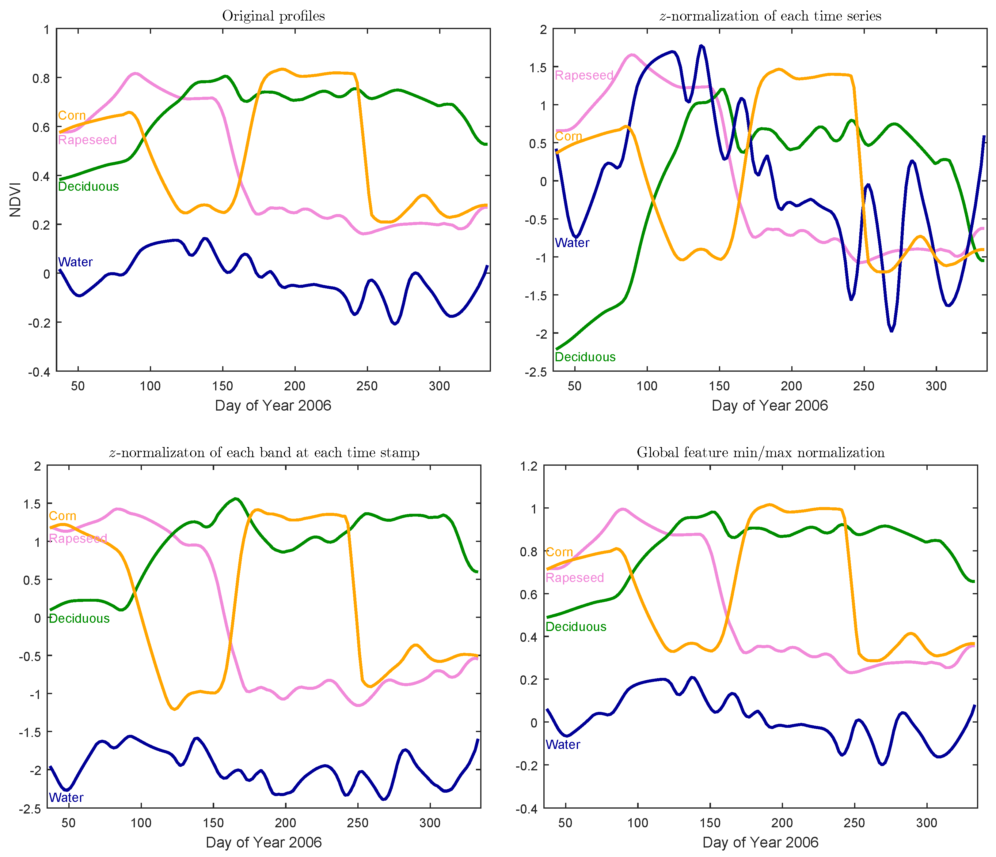
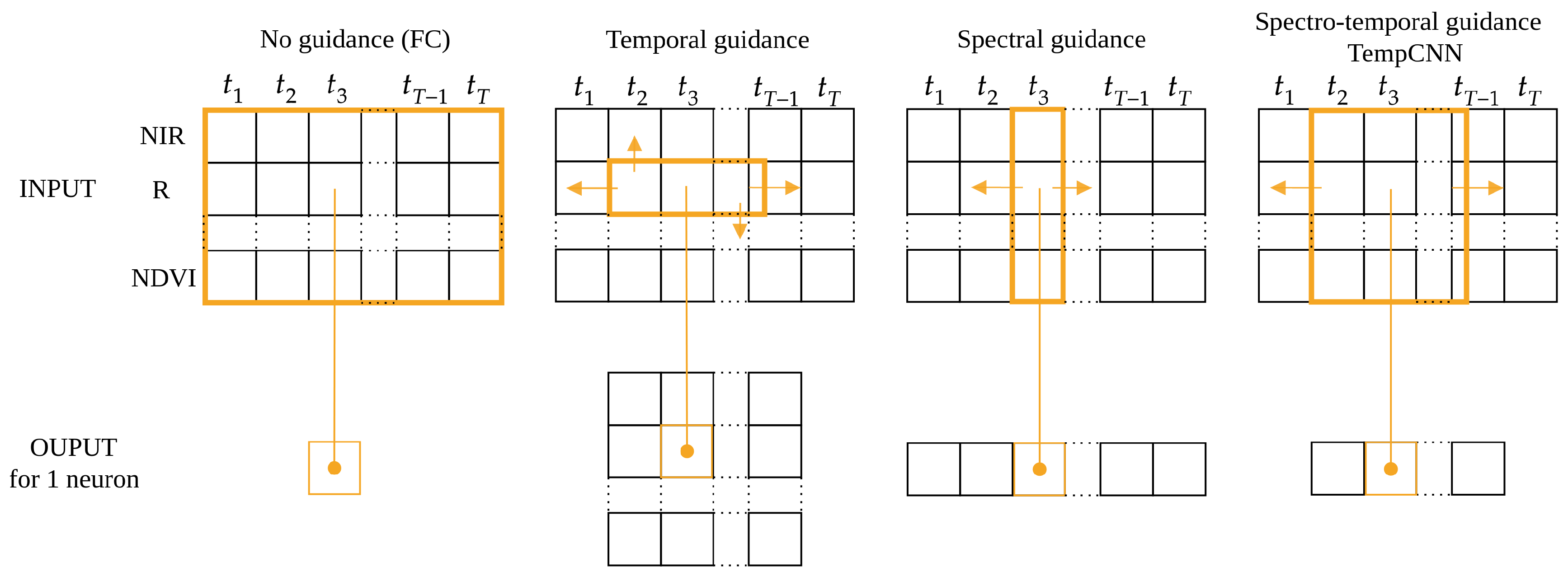
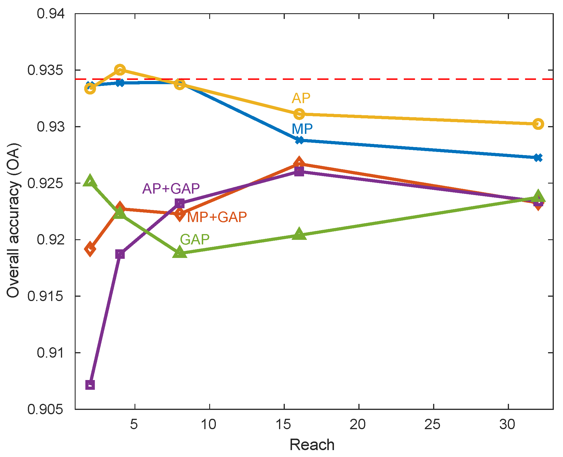
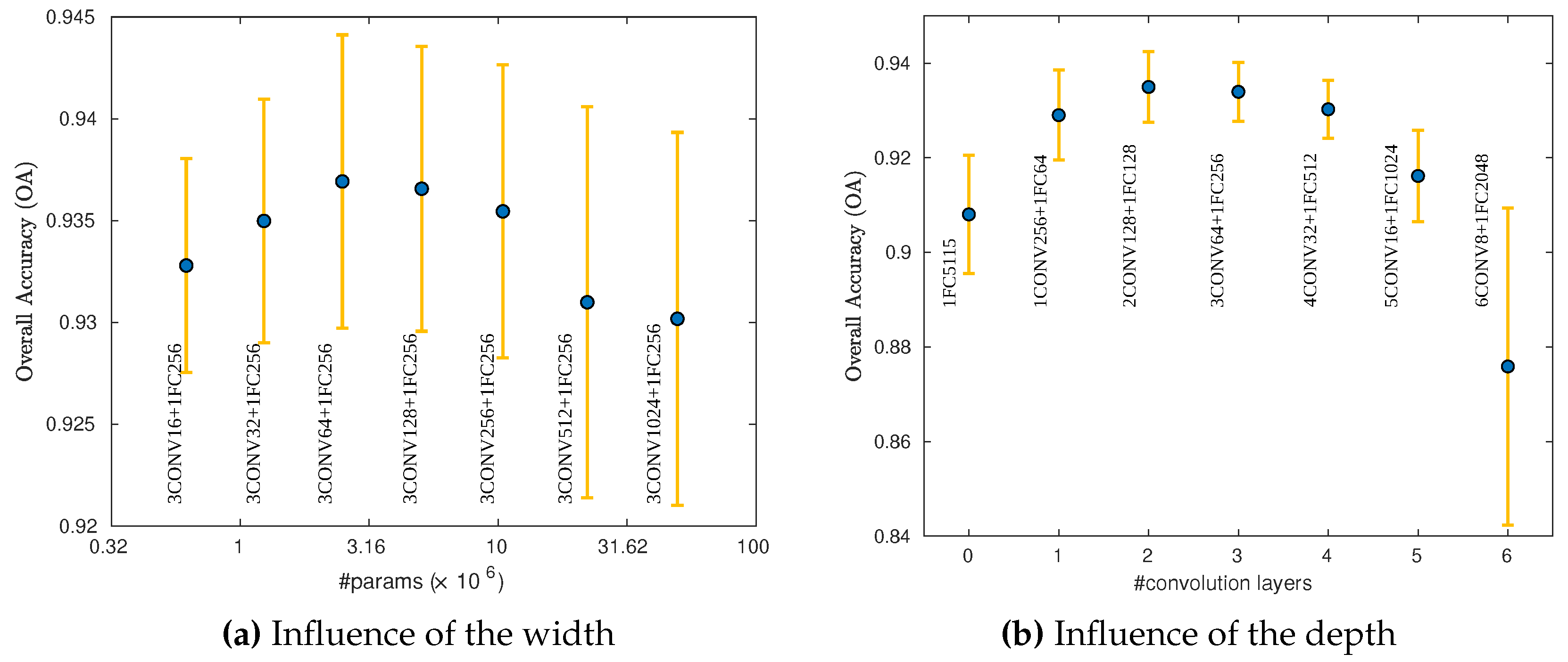
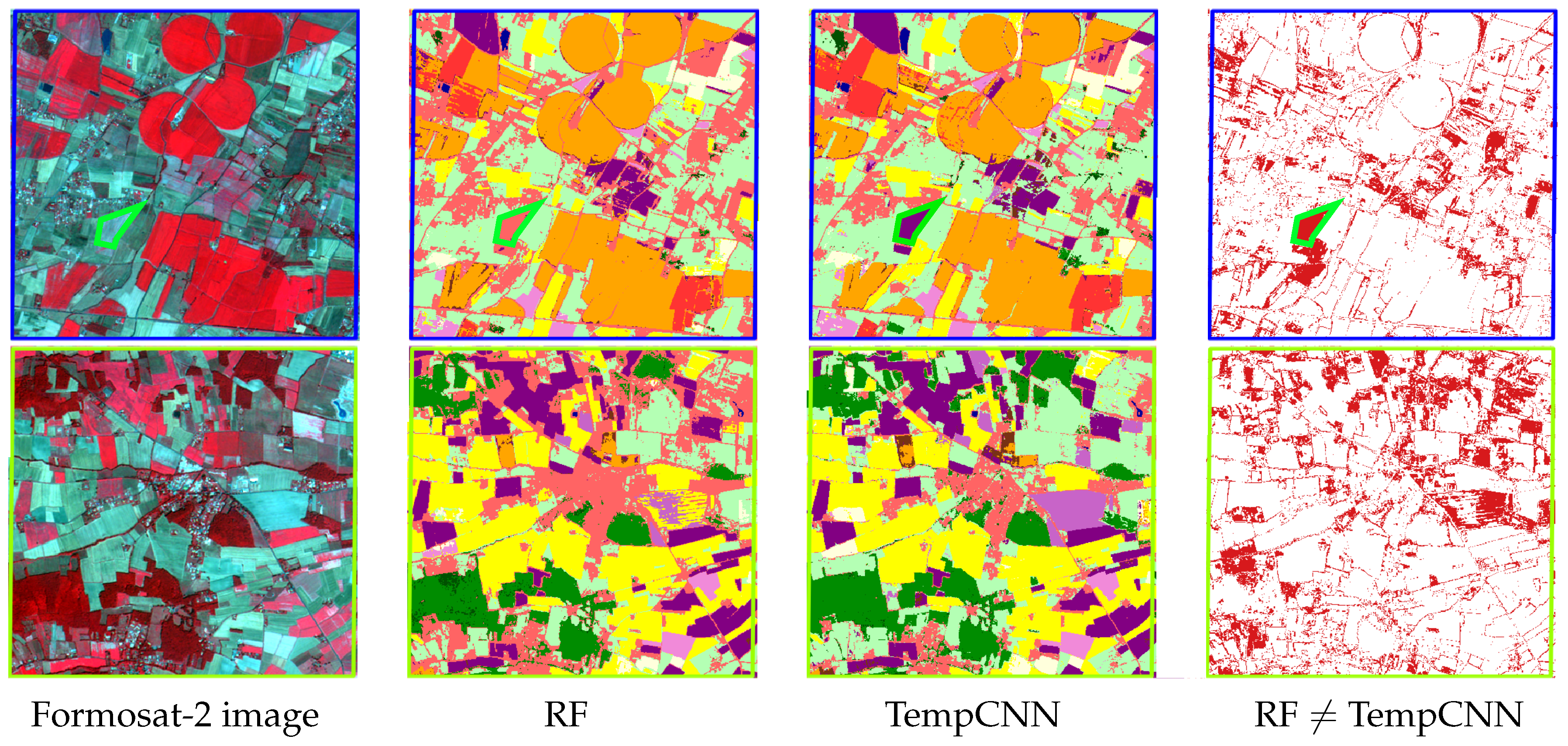
Table 1.
Number of instances per class counted at pixel- and polygon-level.
| Classes | Pixels | Polygons | Legend |
|---|---|---|---|
| Wheat | 194,699 | 295 |  |
| Barley | 23,404 | 43 |  |
| Rapeseed | 36,720 | 55 |  |
| Corn | 62,885 | 83 |  |
| Soy | 9481 | 24 |  |
| Sunflower | 108,718 | 173 |  |
| Sorghum | 17,305 | 22 |  |
| Pea | 9151 | 15 |  |
| Grassland | 202,718 | 328 |  |
| Deciduous | 29,488 | 24 |  |
| Conifer | 15,818 | 18 |  |
| Water | 30,544 | 32 |  |
| Urban | 292,478 | 307 |  |
| Total | 1,033,409 | 1419 |
Table 2.
Number of features () for the studied dataset with T the length of the time series, and D the number of spectral features.
Table 2.
Number of features () for the studied dataset with T the length of the time series, and D the number of spectral features.
| Temporal Sampling | NDVI | SB | SB-NDVI-NDWI-IB | |
|---|---|---|---|---|
| D = 1 | D = 3 | D = 6 | ||
| original | 46 | 138 | 276 | |
| 2 days | 149 | 447 | 894 |
SB: Spectral Bands, NDVI: Normalized Difference Vegetation Index, NDWI: Normalized Difference Water Index, IB: Brilliance Index.
Table 3.
Averaged overall accuracy (± one standard deviation) over five folds for four levels of help in spectral and/or temporal dimensions. Three feature vectors are used here: (1) Normalized Difference vegetation index (NDVI), (2) spectral bands (SB), and (3) SB and three spectral features (SB-SF). Bold values show the highest performance for each type of features. CNN/ COnvolutional Neural Network.
| NDVI | SB | SB-SF | ||
|---|---|---|---|---|
| No guidance | Random Forest (RF) | 88.17 ± 0.59 | 90.02 ± 1.44 | 90.92 ± 1.22 |
| Fully-Connected (FC) | 86.90 ± 1.65 | 91.36 ± 1.15 | 91.87 ± 0.88 | |
| Recurrent Neural Network (RNN) | 88.62 ± 0.86 | 92.18 ± 1.43 | 92.38 ± 0.83 | |
| CNN with temporal guidance | 90.16 ± 0.94 | 92.74 ± 0.80 | 93.00 ± 0.83 | |
| CNN with spectral guidance | 88.24 ± 0.63 | 93.34 ± 0.88 | 93.24 ± 0.83 | |
| CNNwith spectro-temporal guidance (TempCNN) | 90.06 ± 0.88 | 93.42 ± 0.76 | 93.45 ± 0.77 | |
Table 4.
Per-class quality measures. PA: producer’s accuracy. UA: user’s accuracy. Bold values represent the highest F-Score per class.
Table 4.
Per-class quality measures. PA: producer’s accuracy. UA: user’s accuracy. Bold values represent the highest F-Score per class.
| RFs | RNNs | TempCNNs | |||||||
|---|---|---|---|---|---|---|---|---|---|
| UA | PA | F-Score | UA | PA | F-Score | UA | PA | F-Score | |
Whe  | 94.53 | 94.86 | 94.70 | 95.03 | 94.75 | 94.89 | 95.21 | 95.97 | 95.59 |
Bar  | 90.08 | 58.49 | 70.92 | 67.28 | 61.52 | 64.27 | 82.59 | 59.90 | 69.44 |
Rap  | 96.52 | 92.70 | 94.57 | 94.86 | 91.26 | 93.02 | 98.34 | 95.61 | 96.96 |
Cor  | 91.74 | 97.43 | 94.50 | 95.24 | 96.02 | 95.63 | 94.04 | 97.55 | 95.76 |
Soy  | 91.82 | 71.52 | 80.41 | 83.36 | 78.52 | 80.87 | 84.83 | 82.86 | 83.83 |
Sun  | 90.09 | 92.15 | 91.11 | 90.02 | 93.27 | 91.62 | 91.02 | 94.56 | 92.76 |
Sor  | 75.02 | 30.66 | 43.53 | 66.14 | 49.66 | 56.73 | 78.02 | 47.13 | 58.77 |
Pea  | 98.91 | 44.42 | 61.30 | 72.20 | 59.22 | 65.07 | 85.66 | 69.93 | 77.00 |
Gra  | 91.54 | 87.01 | 89.22 | 92.49 | 93.69 | 93.09 | 92.84 | 94.92 | 93.87 |
Dec  | 81.09 | 68.18 | 74.08 | 78.79 | 75.74 | 77.24 | 79.57 | 74.18 | 76.78 |
Con  | 52.55 | 49.01 | 50.71 | 57.56 | 56.05 | 56.79 | 54.48 | 59.45 | 56.86 |
Wat  | 99.90 | 99.02 | 99.46 | 99.21 | 97.92 | 98.56 | 99.81 | 99.69 | 99.75 |
Urb  | 86.47 | 99.66 | 92.60 | 96.48 | 98.92 | 97.68 | 97.16 | 99.31 | 98.22 |
Table 5.
Averaged Overall Accuracy (OA), ±one standard deviation, and F-Score values for five reach values. Bold values highlights the highest values.
Table 5.
Averaged Overall Accuracy (OA), ±one standard deviation, and F-Score values for five reach values. Bold values highlights the highest values.
| Reach | 2 | 4 | 8 | 16 | 32 |
|---|---|---|---|---|---|
| Whe | 95.47 | 95.58 | 95.67 | 95.48 | 95.30 |
| Bar | 68.17 | 69.39 | 69.44 | 68.75 | 68.29 |
| Rap | 96.76 | 96.93 | 96.73 | 96.58 | 95.58 |
| Cor | 95.58 | 95.77 | 96.65 | 96.41 | 96.18 |
| Soy | 82.79 | 83.78 | 83.97 | 82.96 | 82.97 |
| Sun | 92.44 | 92.76 | 92.82 | 92.74 | 92.87 |
| Sor | 54.58 | 58.77 | 61.87 | 62.00 | 61.20 |
| Pea | 74.64 | 77.01 | 75.24 | 68.14 | 69.79 |
| Gra | 93.82 | 93.85 | 93.95 | 93.17 | 92.86 |
| Dec | 76.78 | 76.65 | 76.46 | 76.13 | 76.83 |
| Con | 56.57 | 56.49 | 54.21 | 53.88 | 53.80 |
| Wat | 99.76 | 99.76 | 99.78 | 99.66 | 99.70 |
| Urb | 98.16 | 98.22 | 98.15 | 97.58 | 97.43 |
| OA | 93.29 ± 0.82 | 93.42 ± 0.76 | 93.43 ± 0.62 | 93.00 ± 0.85 | 92.79 ± 0.72 |
Table 6.
Averaged overall accuracy over five runs using different regularization techniques. The first and last rows display Overall Accuracy when all the regularization techniques are turned off and on, respectively. The used dataset is composed of three spectral bands with a regular temporal sampling at two days.
| Overall Accuracy | |
|---|---|
| Nothing | 90.83 ± 0.82 |
| Only dropout | 93.12 ± 0.64 |
| Only batch normalization | 92.22 ± 0.86 |
| Only validation set | 91.17 ± 0.94 |
| Only weight decay | 90.74 ± 1.00 |
| All except dropout | 92.07 ± 1.20 |
| All except batch normalization | 92.89 ± 0.72 |
| All except validation set | 93.68 ± 0.60 |
| All except weight decay | 93.52 ± 0.77 |
| All | 93.42 ± 0.76 |
Table 7.
Training time and averaged Overall Accuracy (OA) over five folds for the same model learned for five batch sizes.
Table 7.
Training time and averaged Overall Accuracy (OA) over five folds for the same model learned for five batch sizes.
| Batch Size | Training Time | OA |
|---|---|---|
| 8 | 3 h 45 min | 93.54 ± 0.67 |
| 16 | 1 h 56 min | 93.65 ± 0.73 |
| 32 | 1 h 06 min | 93.59 ± 0.74 |
| 64 | 34 min | 93.43 ± 0.71 |
| 128 | 19 min | 93.45 ± 0.83 |
© 2019 by the authors. Licensee MDPI, Basel, Switzerland. This article is an open access article distributed under the terms and conditions of the Creative Commons Attribution (CC BY) license (http://creativecommons.org/licenses/by/4.0/).
Share and Cite
MDPI and ACS Style
Pelletier, C.; Webb, G.I.; Petitjean, F. Temporal Convolutional Neural Network for the Classification of Satellite Image Time Series. Remote Sens. 2019, 11, 523. https://0-doi-org.brum.beds.ac.uk/10.3390/rs11050523
AMA Style
Pelletier C, Webb GI, Petitjean F. Temporal Convolutional Neural Network for the Classification of Satellite Image Time Series. Remote Sensing. 2019; 11(5):523. https://0-doi-org.brum.beds.ac.uk/10.3390/rs11050523
Chicago/Turabian StylePelletier, Charlotte, Geoffrey I. Webb, and François Petitjean. 2019. "Temporal Convolutional Neural Network for the Classification of Satellite Image Time Series" Remote Sensing 11, no. 5: 523. https://0-doi-org.brum.beds.ac.uk/10.3390/rs11050523
Note that from the first issue of 2016, this journal uses article numbers instead of page numbers. See further details here.