Article

An Uncertainty Quantified Fundamental Climate Data Record for Microwave Humidity Sounders

1
Meteorologisches Institut, Centrum für Erdsystem- und Nachhaltigkeitsforschung (CEN), Universität Hamburg, Bundesstrasse 55, 20146 Hamburg, Germany
2
EUMETSAT, Eumetsat Allee 1, 64295 Darmstadt, Germany
*
Author to whom correspondence should be addressed.
Submission received: 29 January 2019 / Revised: 23 February 2019 / Accepted: 26 February 2019 / Published: 6 March 2019
(This article belongs to the Special Issue Assessment of Quality and Usability of Climate Data Records)

Abstract

:
To date, there is no long-term, stable, and uncertainty-quantified dataset of upper tropospheric humidity (UTH) that can be used for climate research. As intermediate step towards the overall goal of constructing such a climate data record (CDR) of UTH, we produced a new fundamental climate data record (FCDR) on the level of brightness temperature for microwave humidity sounders that will serve as basis for the CDR of UTH. Based on metrological principles, we constructed and implemented the measurement equation and the uncertainty propagation in the processing chain for the microwave humidity sounders. We reprocessed the level 1b data to obtain newly calibrated uncertainty quantified level 1c data in brightness temperature. Three aspects set apart this FCDR from previous attempts: (1) the data come in a ready-to-use NetCDF format; (2) the dataset provides extensive uncertainty information taking into account the different correlation behaviour of the underlying errors; and (3) inter-satellite biases have been understood and reduced by an improved calibration. Providing a detailed uncertainty budget on these data, this new FCDR provides valuable information for a climate scientist and also for the construction of the CDR.

Graphical Abstract

1. Introduction

We constructed a new fundamental climate data record (FCDR) that stores the brightness temperature measured by the microwave humidity sounders Special Sensor Microwave Water Vapor Profiler (SSMT-2), Advanced Microwave Sounding Unit-B (AMSU-B) and Microwave Humidity Sounder (MHS) installed on board polar orbiting satellites. This FCDR overcomes certain problems of the available historical operational data of these instruments, which were not designed for climate monitoring, but for assimilation in numerical weather prediction (NWP). As these datasets now cover more than 20 years, they become increasingly relevant for climate science. Climate research requires long-time, consistent and uncertainty-quantified data records that the available operational datasets do not provide. New aspects of our FCDR are: (1) easy handling and removal of sampling artefacts originating from overlapping orbit files; (2) extensive pixel-level uncertainty information considering correlation behaviour of the underlying errors—a strategy based on metrological principles; and (3) understanding and reducing inter-satellite biases by an improved calibration. The new FCDR shall serve as a starting point for the construction of a climate data record (CDR). The CDR will be a gridded dataset containing the essential climate variable (ECV) upper tropospheric humidity (UTH). UTH is an important ECV to be monitored: water vapour is a major greenhouse gas that is highly variable in space and time. Hence, global continuous observations are required for which satellite borne measurements are of high interest. Another application of the new FCDR is the assimilation into reanalyses.
The available operational data of these microwave humidity sounders exhibit certain problems that prevent the application of the data for climate monitoring thus far: the handling of the operational data for scientific studies is tedious because doubled data resulting from overlaps of subsequent orbit files create artefacts that need to be filtered out by the users.
Furthermore, the operational data only contain very sparse information on uncertainty. Only the noise equivalent differential temperature (NE Δ T) is provided for some instruments. No information on other uncertainties in the measurement process are reported or propagated to brightness temperature. However, full uncertainty information is required. Especially those uncertainties associated with systematic errors in the brightness temperature need to be characterised. Uncertainties associated with systematic effects are the most important uncertainties on longer time scales as they cannot be reduced by averaging as the random ones (NE Δ T) can. Hence, for constructing a gridded CDR product, based on averaged data, detailed uncertainty information is crucial for propagating the uncertainty to the ECV stored in the CDR and for communicating the trust in observed quantities and their evolution.
To obtain a consistent, long-term record of an ECV and to prevent misinterpretation of instrumental changes as changes of the climate system, the stability of the underlying FCDR is most important. However, the operational data show biases for the instruments flown on different satellites, thus preventing the construction of stable data records. Estimates of the observed inter-satellite biases vary slightly depending on the method used to compare the instruments, particularly when they are on satellites with different local equator crossing times (LECT). This is because the methods use a different sampling of the data: simultaneous nadir overpasses (SNOs) make use of (almost) simultaneous measurements of (almost) the same target by two instruments. Hence, they are not affected by diurnal cycle effects. These diurnal cycle effects do, however, affect methods using averaged data, such as monthly zonal or global averages. Consequently, the inter-satellite biases may vary depending on the method. Nonetheless, there is overall agreement of the methods on very strong, time dependent, increasing biases of several kelvin for AMSU-B on NOAA-15 and on NOAA-16 against MHS on NOAA-18 for the sounding channels [1,2]. MHS on NOAA-19 also shows a strong bias against NOAA-18 [2]. AMSU-B on NOAA-17 as well as the MHS on Metop-A and Metop-B only show small biases against NOAA-18 in the sounding channels [2]. These biases, which depend on time, scan angle and brightness temperature, prevent a construction of stable, consistent time series and require dedicated efforts to reconcile the instruments.
Previous efforts to achieve this reduction of the biases and to inter-calibrate microwave sounders were only bias corrections. That means an offset was determined [2], a slope and an off-set were determined [3], or an offset and a non-linearity were determined [4] (for the MSU (Microwave Sounding Unit) instrument) to reduce the bias in brightness temperature. A recent attempt used interpolation to produce look-up tables with calibration coefficients that change from month to month in order to reconcile the AMSU-B and MHS sensors [5]. Chung et al. [6] also inter-calibrated AMSU-B and MHS instruments using a zonal-average method for adjusting inter-satellite differences as in [7]. The obtained inter-calibrated dataset shows improved consistency between the instruments [8]. In addition, inter-calibration efforts were undertaken for the SSM/I instrument (Special Sensor Microwave Imager), and an FCDR was produced as basis for CDRs of precipitation and evaporation (e.g., [9,10,11,12]). Zou et al. [13] and Mo [14] inter-calibrated AMSU-A instruments to obtain bias-free datasets. For climate studies, such datasets are essential for all Earth-observation instruments, and the list of mentioned efforts for the inter-calibration of various instruments makes no claim to completeness. In [15], an overview is given of the inter-calibration methods to detect biases, and the corresponding publications. An inter-calibrated dataset allows for bias-reduced time series. However, the inter-calibration by bias correction does not necessarily lead to an understanding of the underlying instrumental effects causing the biases, but only corrects for their final impact on the brightness temperature.
Our approach for the AMSU-B and MHS sensors is to analyse the biases and understand their origin in order to mitigate their effect by a recalibration procedure, leading to a consistent FCDR. This recalibration is based on a metrology inspired measurement equation approach. This effort is undertaken in the Horizon 2020 project FIDUCEO.

2. Data and Methods

2.1. Microwave Radiometer Data

This study focused on the three cross-track scanning microwave humidity sounders MHS, AMSU-B and SSMT-2. Over the considered time period of 1994–2017, there were eleven individual instruments of this family (see Table 1): the first microwave humidity sounder was SSMT-2 on the Defense Meteorological Satellite Program (DMSP) F11 satellite. It was followed by three further SSMT-2 instruments on board the F12, F14 and F15 satellites. The first AMSU-B instrument was launched on NOAA-15 satellite in 1998 by National Oceanic and Atmospheric Administration (NOAA). Two further AMSU-B instruments followed on NOAA-16 and NOAA-17 satellite. The MHS instrument was first launched on board the NOAA-18 satellite in 2005. To date, three further MHS instruments have been launched on NOAA-19 and on Metop-A and Metop-B satellites controlled by EUMETSAT (the fifth MHS on Metop-C was launched only very recently in November 2018 and is not part of this study). We produced a consistent, stable FCDR for microwave humidity sounders including all SSMT-2, AMSU-B and MHS. In some detailed aspects of the calibration, our work mainly focused on the AMSU-B and MHS instruments, for which the required information is available in contrast to SSMT-2. However, the consistent application of the measurement equation (see Section 2.2.1) as well as the uncertainty quantification of the FCDR is also in place for SSMT-2, leading to an improved data record (see Section 3.4).
The three instruments are very similar in their scanning mode, calibration procedure and in spectral characteristics. The instruments have five spectral channels, three of which are sounding channels sensitive to water vapour absorption at different altitudes. Two further channels detect radiation from deeper layers of the atmosphere and from the surface. Table 2 summarises key characteristics of the instruments (data taken from [16,17]). Kobayashi et al. [17] gave a detailed table on the instrumental characteristics. The most interesting channel in terms of the UTH is the channel at 183 ± 1 GHz, closely positioned around the strong water vapour absorption line.
We used uncalibrated level 1b data from the NOAA CLASS (Comprehensive Large Array-data Stewardship System) archive, covering the missions of the eleven individual instruments. Note, however, that only the NOAA NCEI (National Centers for Environmental Information, formerly NGDC, National Geophysical Data Center) archive actually stores the entire record of the SSMT-2 missions. However, this record does not provide the raw digital counts and the calibration information of the temperature of the internal target for example. Since we needed this information for the recalibration, we used the NOAA CLASS archive data only, as we did for the AMSU-B and MHS instruments. Consequently, our SSMT-2 FCDR is restricted in time: e.g., it only starts in 1994 instead of 1992. Table 1 shows the time range of our new FCDR data. Moreover, several data gaps exist in the NOAA CLASS SSMT-2 records. Hence, our SSMT-2 FCDR also exhibits these gaps. From the level 1b files, all information and data necessary for recalibration are read in our new processing chain.

2.2. Methods

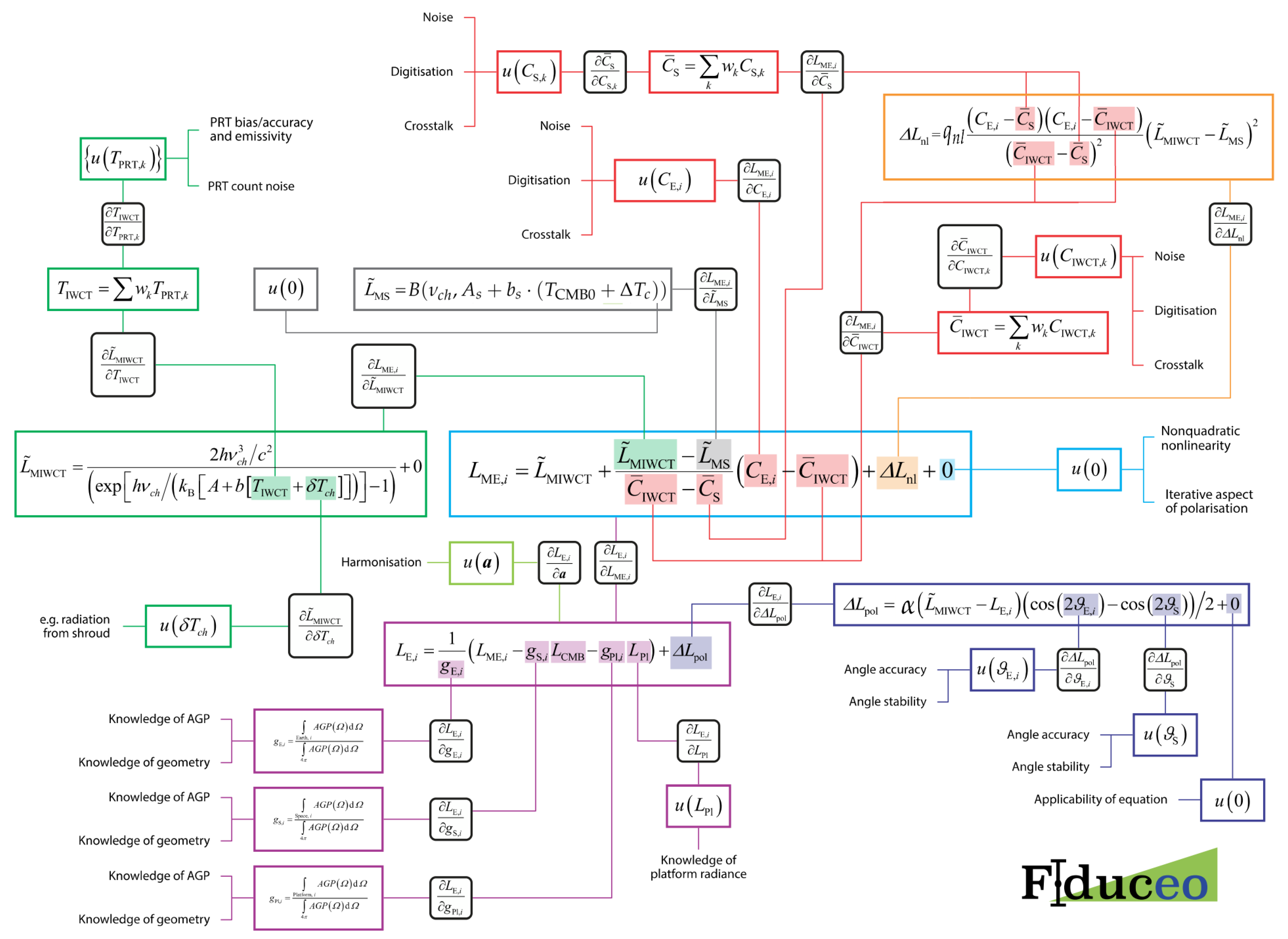
2.2.1. Measurement Equation Approach

The operational calibration of these instruments’ data (the level 1b to level 1c processing) was done by a software package called AAPP (ATOVS (Advanced TIROS-N (Television InfraRed Operational Satellite—Next-generation) Operational Vertical Sounder) and AVHRR (Advanced Very High Resolution Radiometer) Pre-processing Package) [18]. We reimplemented this entire processing chain, following the AAPP equations in general, but allowing for possible changes to improve the calibration (see Section 2.2.2 for the applied improvements). Improving the calibration was the main goal to produce a consistent FCDR of reduced inter-satellite biases.
The processing chain for transforming the raw data to the FCDR included the calibration of the instrument. Inspired by the discipline of metrology, we used a rigorous measurement equation approach for formulating the calibration. Contentwise, the calibration was the same as in AAPP (before we applied our improvements, see Section 2.2.2). The formulation, however, was more instrument-oriented in the sense that all corrections appear explicitly and are not absorbed in higher-level calibration coefficients. This facilitated the uncertainty analysis. The measurement equation concept is described in detail in [19]. In short, the measurement equation for the considered microwave (MW) instruments is an analytical expression that relates all quantities required to model the measurement process and to translate the raw digital counts to brightness temperature.
For the MW radiometers, the basic measurement equation is a two point calibration that interpolates between a known cold and warm calibration target to obtain the calibrated signal of the observed target. The deep space view (DSV) serves as cold target (cosmic microwave background). A black body whose temperature is constantly measured by several platinum resistance thermometers (PRTs) forms the internal warm calibration target (IWCT). Hence, the basic measurement equation for the two point calibration reads
L E = L IWCT + L IWCT L S C IWCT C S · ( C E C IWCT ) ,
where L stands for radiance and C for count. The indices IWCT, S and E denote the internal warm calibration target, space and Earth, respectively.
Building the full measurement equation required for a comprehensive propagation of uncertainties requires an assessment of all possible effects that have an impact on the measurement process and that were considered in the operational calibration by AAPP. The full AAPP measurement equation is presented in Figure 1 as diagram indicating all dependencies. The final Earth radiance L E is calculated from
L E = 1 1 g S g Pl 1 2 B ( ν c h , A + b · ( T ¯ IWCT + δ T c h ) ) + B ( ν c h , A + b · ( T ¯ IWCT + δ T c h ) ) B ( ν c h , A s + b s · ( T CMB 0 + Δ T c ) ) C ¯ IWCT C ¯ S · ( C E C ¯ IWCT ) + q n l ( C E C ¯ S ) · ( C E C ¯ IWCT ) ( C ¯ IWCT C ¯ S ) 2 · [ B ( ν c h , A + b · ( T ¯ IWCT + δ T c h ) ) B ( ν c h , A s + b s · ( T CMB 0 + Δ T c ) ) ] 2 g S · B ( ν c h , A s + b s · ( T CMB 0 ) ) g Pl L Pl 1 2 + α [ B ( ν c h , A + b · ( T ¯ IWCT + δ T c h ) ) L E ] · 1 2 ( cos 2 θ E cos 2 θ S ) ,
where B is the Planck function and ν c h is the frequency of the channel, e.g., in the case of AMSU-B, it is 89 GHz, 150 GHz and 183.31 GHz for channels 1, 2 and 3–5, respectively. All further used symbols and quantities are explained in the following, in the context of the effect that they model.
The effect of noise affects the measured Earth counts C E , space counts C S and IWCT counts C IWCT . In addition, the measured temperature of the IWCT T IWCT is subject to noise. These quantities (except for C E ) appear as averaged values in the measurement equation: for each scan, four samples of the DSV and IWCT view were averaged. Furthermore, a weighted rolling average over seven scan lines was computed for each scan line, resulting in C ¯ IWCT and C ¯ S . The same procedure was executed for the temperature of the black body. The temperature was measured by five, seven or two PRT sensors for MHS, AMSU-B and SSMT-2, respectively. After averaging these samples for each scan line, the weighted rolling average was applied, finally yielding T ¯ IWCT . This procedure was for noise reduction [20].
The coefficients g S and g Pl denote the contribution of space and platform, respectively, to the overall measured signal in the Earth views:
1 = g E + g S + g Pl
These coefficients form the antenna pattern correction that accounts for the fact that radiation from space and platform is detected in the side lobes of the antenna. The coefficients are determined pre-launch by convolving the measured antenna pattern with a geometrical map of the instruments’ environment on board the satellite [21,22]. Since both the geometry of the instruments’ environment and the measured antenna pattern influence the antenna pattern correction, the uncertainties of both components translate into the uncertainty of the antenna pattern correction. An inaccurate knowledge of both components causes uncertainties, especially if the antenna efficiency is low. The main beam efficiency for AMSU-B was measured as 94.4%, 95.1% and 96.9% for channels 1, 2 and 4 of NOAA-15, respectively (for further values, see also [21]). No values for the uncertainties of either component were known, which was a reason to use rather large estimates (see Section 2.2.3). Moreover, we detected a wrong assignment of the antenna pattern correction to the channels for the AMSU-Bs and the MHS on NOAA-18 within the fdf.dat calibration file of AAPP [18]. Erroneously, channel 4 and 5 received the corrections for channel 1 and 2, respectively, instead of receiving the correction for channel 3. Note that the sounding channels of AMSU-B share the same quasi-optical path and should therefore receive the same antenna pattern correction.
The radiance of the platform L Pl itself is not known. Hence, it must be approximated. In [21], the radiance of the platform is assumed to be equal to the concurrently-measured Earth radiance. This appears as an oversimplification. Using the opposite, cold extreme of the cosmic microwave background being reflected by the platform results in a change of about 0.22 K in the affected pixels at the edge of the swath, compared to the warm extreme of assuming reflected Earth radiance. This result was obtained for channel 1, which has the largest antenna pattern correction and hence largest influence from L Pl . For channel 3, which has a much smaller antenna pattern correction, the change is only about 0.03 K. Since this is a very small change from one extreme assumption to the other, the choice of applied assumption is less important (but should be kept in mind for channel 1). Hence, we used the approximation of Hewison and Saunders [21], which is also used in the operational calibration by AAPP.
Similar to the Earth views, the DSVs may be affected by radiation entering the side lobes. This is corrected for by a simple additive correction Δ T c to the pure cosmic microwave background T CMB 0 :
T CMB 0 + Δ T c
The correction Δ T c is determined during the in-orbit verification phase [22,23,24,25]. The correction enters the measurement equation as
L ˜ MS = B ( v c h , A s + b s ( T CMB 0 + Δ T c ) ) .
The same type of correction is applied to the IWCT view
T ¯ IWCT + δ T c h .
The correction enters the measurement equation as
L ˜ MIWCT = B ( v c h , A + b ( T IWCT + δ T c h ) ) .
All channels and instruments only have zero valued δ T c h , except for channel 20 of AMSU-B on NOAA-17 (see AAPP auxiliary files: clparams.dat, [18]). The correction accounts for all effects that change the emitted radiation in the IWCT view that is otherwise only characterised by the temperature of the black body. This correction includes undetected vertical thermal gradients across the black body. Note that the black body is an array of pyramidal tines of aspect ratio 4:1 [20]. Since the PRTs are placed on the back side of the black body, while the antenna receives radiation emitted from the front side, a thermal gradient across the pyramidal structure might be a source of error. However, it is very small [26]. The correction δ T c h also accounts for the radiation from the shroud of the black body that might have a slightly different temperature than the black body itself [27,28].
The coefficient α is part of the polarisation correction. This correction accounts for the different reflectivities of the mirror for horizontally and vertically polarised radiation, combined with the polarisation sensitivity of the channels. The correction reads
α [ B ( ν c h , A + b · ( T ¯ IWCT + δ T c h ) ) L E ] · 1 2 ( cos 2 θ E cos 2 θ S ) .
The correction depends on the scan angle and the position of the DSV (angles for Earth view θ E and for space view θ S ). α is included in the fdf.dat files from AAPP. For unclear reasons, however, α is non-zero only for MHS on NOAA-18, although a correction scheme similar to Equation (8) had been devised for AMSU-B in pre-launch tests [20]. Strictly speaking, this polarisation correction needs to be executed iteratively as it depends on the measured Earth radiance. As approximation, we used the calibrated Earth radiance L E without the polarisation correction to then compute L E using the polarisation correction.
The basic measurement equation is a linear model only. To account for possible non-linearity, the non-linearity coefficient q n l is introduced with a second order term in C E . The values for this q n l are stored in the clparams.dat file in AAPP. The origin of the values is not clear. They were probably obtained during pre-launch tests. However, the information is not traceable and not consistent with results from ground tests done by Matra Marconi for demonstrating compliance with requirements [29].
The coefficients A , b and A s , b s are band correction factors. The channels do not measure at one frequency, but they measure an average of the signal in two pass bands placed at slightly higher and slightly lower frequencies around ν c h = 89, 150 or 183.31 GHz. Consequently, the monochromatic assumption in using the Planck function at a single frequency breaks down for the channels at 183.31 ± 3 GHz and at 183.31 ± 7 GHz, for which the two pass bands are significantly separated. To account for this, the band correction factors A and b have been introduced in AAPP.
Another effect is the radio frequency interference (RFI) from on board transmitters. This effect is not captured by the calibration and hence not part of the measurement equation. RFI affects the raw input counts C and therefore needs correction on this low level. RFI is known for the AMSU-B on NOAA-15 [23,30] and receives a correction scheme in AAPP. However, this scheme was not updated over the years, since the RFI changed erratically. Therefore, the later data of AMSU-B on NOAA-15 probably suffer from RFI.
The effects described above are included in the AAPP measurement equation. As indicated already, some of the parameter values used within AAPP are of unclear origin or wrongly assigned. Hence, our goal was to improve the calibration by correcting these parameters.

2.2.2. Improvements Compared to AAPP

Having reimplemented the entire processing chain for the MW sounders, we were ready to change aspects within the calibration that required improvement. Mostly, this refers to improving certain parameter values within the measurement equation.

Antenna Pattern Correction (APC)

In AAPP, the APC is stored for the AMSU-B and MHS instruments in the auxiliary fdf.dat file, providing values for g E , g Pl , g S .
As explained above, we detected wrong assignments of values to channels: for the AMSU-B instruments the sounding channels 3–5 should all receive the same APC (instead of channel 4 receiving channel 1 APC and channel 5 receiving channel 2 APC). This error was corrected in our new FCDR processing for AMSU-B on NOAA-15, -16 and -17. This affected channels 4 and 5.
Per default in AAPP, MHS on Metop-A receives the APC of NOAA-15. However, this can be changed manually to the correct APC provided by EUMETSAT (as indicated in the fdf.dat file). In our FCDR processing, we only used the correct APC for Metop-A. This affected all channels.
In AAPP, MHS on NOAA-18 receives the APC from AMSU-B on NOAA-15. No other APC is provided for NOAA-18 in AAPP. This assignment of NOAA-15 APC to NOAA-18 is problematic, since it does not take into account the change of instrument. To achieve a first improvement on this, while considering the instrument and the satellite that both influence the APC, we used in our FCDR processing the APC of MHS on NOAA-19 for the MHS on NOAA-18. This affected all channels.
Note that SSMT-2 does not receive an APC in the operational calibration. Since we have no information on either the antenna pattern or the surroundings of the instrument on board the DMSP satellites, we could not derive any APC and therefore did not apply an APC to SSMT-2, either. This is reflected in the uncertainties assigned to SSMT-2 in our FCDR.

Band Correction

The band correction coefficients A , b are provided in AAPP to be used in the IWCT views of channels 4 and 5 for AMSU-B and for channel 4 of MHS. We determined new coefficients A s , b s to account for the same effect in the DSV for which the same values as for the IWCT were erroneously used in AAPP. A s , b s were obtained such that the deviation was minimised between the radiance computed by the Planck function evaluated at ν c h for a modified temperature A s + b s · T and the average of the radiances computed by the Planck function evaluated at the upper ( ν c h + d ν c h ) and lower ( ν c h d ν c h ) pass band at temperature T, with T = 3 K representing the signal in the DSV. With the same procedure, but using T = 280 K, we also slightly improved A , b for the IWCT views.
Note that SSMT-2 did not receive this band correction in the operational calibration. This was changed in our FCDR processing. SSMT-2 now receives the same band correction coefficients as AMSU-B.

Usage of PRT No. 6 for AMSU-B

In AAPP, PRT No. 6 is always excluded from the computation of the black body temperature (it has weight zero in the clparams.dat file). This is due to a bias that was observed pre-launch. However, we could not find indications of such a bias in the in-flight data. Hence, in our FCDR processing, all PRTs are used per default, but single PRTs may be excluded based on dedicated quality checks. Those quality checks control the spread of the PRTs and the stability of individual PRTs.

Radio Frequency Interference (RFI)

RFI was observed for the AMSU-B on NOAA-15 during the in-orbit verification phase [23,30]. A correction scheme was devised that was, however, not updated in later years as it would have been required. Hence, uncorrected RFI impact is highly probable in NOAA-15 data. For NOAA-16, the RFI measured pre-launch was below the noise level of the instrument and therefore not corrected. However, a growing influence of RFI due to a decreased gain is suggested in [31]. NOAA-17 was only slightly affected and received a small correction for channels 3 and 4 in AAPP.
A dedicated study presented in a different article [32] revealed that also AMSU-B on NOAA-16 and even MHS on NOAA-19 suffer significantly from RFI. RFI was identified as the main reason for the strong inter-satellite biases that are observed for channels 3–5 for AMSU-B on NOAA-16 and 3 and 4 for MHS on NOAA-19. In the same study, we derived a correction scheme to reduce the effect of RFI. This correction scheme was based on global monthly means that were investigated as function of the scan angle against the reference instrument on NOAA-18. For each scan angle and for each period of constant RFI pattern, a correction on the Earth view counts was derived. In our FCDR processing, we applied this correction scheme to the raw counts for NOAA-16 and NOAA-19 and executed the calibration on these RFI-corrected input counts. For NOAA-15 and NOAA-17, we applied an early version of the derived correction scheme (it is more difficult for these instruments to find a good correction scheme, see [33]). The applied RFI correction in our FCDR affected the sounding channels 3–5. Channels 1 and 2 are not RFI-corrected in our FCDR and therefore include the full RFI impact (which is only significant for AMSU-B on NOAA-15 channel 2). The correction scheme could not be derived for these channels with the applied method because these channels are very sensitive to the diurnal cycle, which changes the observed inter-satellite difference.

Accurate Value for Cosmic Microwave Background ( T CMB 0 )

In AAPP, the value of the cosmic microwave background is rounded to 2.73 K (clparams.dat, [18]). In the FIDUCEO FCDR processing, we used the more accurate value of 2.72548 K [34].

2.2.3. Uncertainty Model

A key aspect of the new FCDR is the extensive information on uncertainty of the measured brightness temperature. To obtain this uncertainty information, all sources of error in the measurement process need to be assessed, and the associated uncertainties need to be estimated and propagated to brightness temperature. Starting from the measurement equation, we estimated the uncertainties u ( x j ) associated with the parameters x j of each modelled effect (there are n modelled effects). Furthermore, we computed the sensitivity coefficients c j for each effect as the corresponding partial derivative of the measurement equation. Finally, we obtained the resulting uncertainty on brightness temperature by applying the Law of Propagation of Uncertainties [19,35]:
u 2 ( L ) = j = 1 n c j 2 u 2 ( x j ) + 2 j = 1 n 1 j = j + 1 n c j c j u ( x j , x j )
The term u ( x j , x j ) denotes the covariance of the parameters x j , x j . When individual parameters x j are uncorrelated, i.e. they do not share a common error effect, the second term is zero. As this is valid for most of the identified effects in the MW case, we assumed this metrologically independent case and hence simplified the uncertainty to
u 2 ( L ) = j = 1 n c j 2 u 2 ( x j ) .
Without existing information on the uncertainty of most of the parameters in the AAPP model, we performed separate analysis on an estimate of the input uncertainties u ( x j ) for each effect. To quantify the uncertainty associated with the noise on receiver counts or PRT measurements, a dedicated study was carried out in [36], using the Allan Deviation, which is a method used in metrology that was recently proposed in this context by Tian et al. [37]. This method was used for on-the-fly computation of the noise in counts during the FCDR processing.
We estimated the uncertainties of the other effects based on the spread of given values for different individual instruments of either the AMSU-B, MHS or SSMT-2 family. Hence, uncertainty estimates of 50% or even 100% were used to cover the spread of a certain calibration parameter over the four individual MHS instruments, for example. More detailed information is given in [28,33], including all partial derivatives.
Apart from providing uncertainty information in the first place, we also considered the different correlation behaviour in space and time of the various effects. A detailed description of the underlying concept is provided in [38]. Here, we briefly present the idea: all effects were classified as independent, structured or common, depending on the correlation scale of the underlying error. The independent effects are composed of the pure random effects (Earth view count noise and random error on angle θ E ). They are not correlated between any pixels across or along track. For the considered MW instruments, the structured effects are of random nature, but the calibration procedure introduces correlation. This is the case for all calibration quantities undergoing the seven-scan line average (DSV, IWCT counts and temperature of the black body). The common effects have correlation scales exceeding one orbit. All calibration parameters that are (assumed) to be constant over the mission are part of this category (non-linearity, polarisation correction, antenna pattern correction, and cold and warm target correction). This classification according to the correlation behaviour allows for an advanced usage of uncertainties in the derivation of higher level products. Since these higher level products often rely on averaging procedures, it is of crucial importance to know which proportion of the uncertainty budget is associated with each correlation scale. For example, the uncertainty due to independent effects can be reduced by averaging, whereas the uncertainty due to common effects cannot. Hence, on longer time scales, which are especially interesting for climate research, the common effects become more dominant.
It is also interesting for users to know the length scales of error correlation within an orbit, giving an indication of the extent of correlation for pixels a given distance apart. Since the structured effects are formed by the seven-scan line average, the overall along track length scale over which the correlation decreases to zero is seven scan lines. Based on the analysis in [19], we assumed a decrease in correlation over the scan lines to be modelled by a Gaussian curve that is truncated for a separation of two scan lines Δ l = l 2 l 1 larger than six scan lines (the variance of this Gaussian is σ 2 = ( 3 / 3 ) 2 following from [19]). This estimation accounts for the fact that the seventh neighbouring scan line will have no calibration quantities in common with the initial scan line and therefore is uncorrelated with the initial scan line. Across track, the errors due to structured effects of all pixels of one scan line are completely correlated as they belong to the same calibration cycle and are therefore subject to the same errors within the calibration quantities of DSV and IWCT view.

3. Results

In the following, we briefly compare the initial implementation of the FCDR processing (without improvements), as well as the final implementation (with improved calibration) to AAPP-processed data. Moreover, we present example contents of our new, improved FCDR, as well as an inter-satellite comparison using operational and FCDR data highlighting the improvements made in the FCDR processing so far.

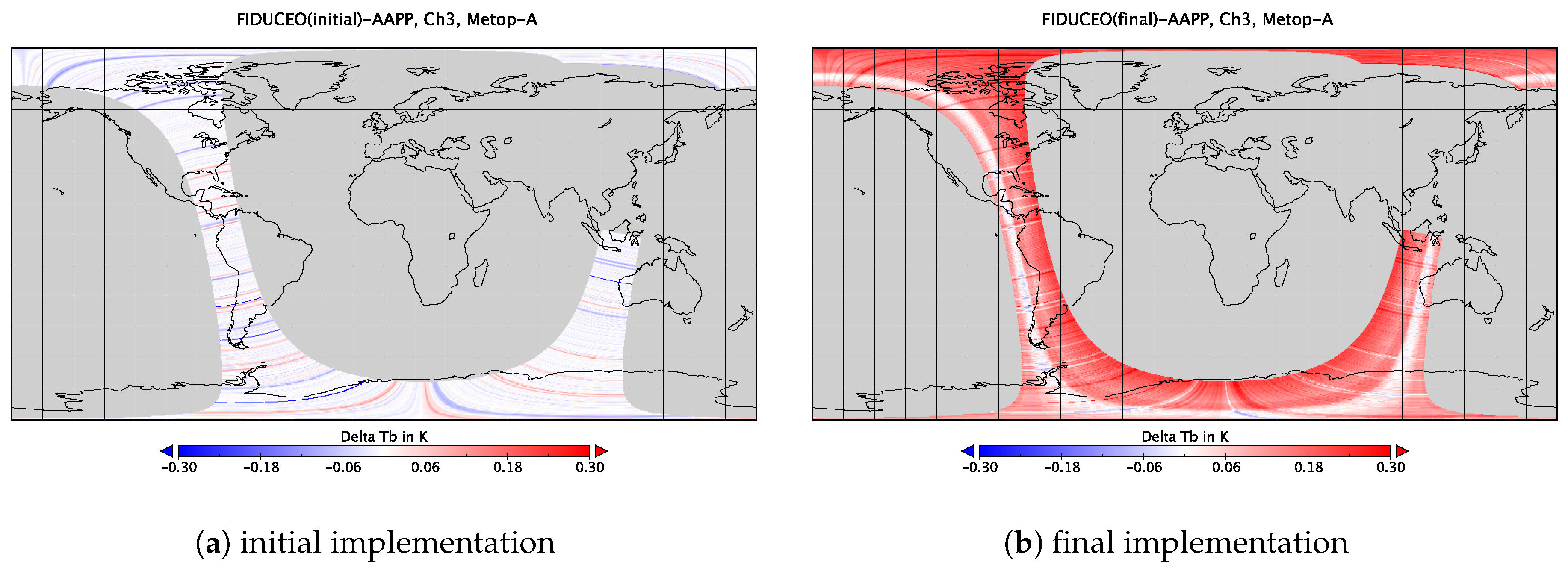
3.1. Comparing the Initial and Final Implementation to AAPP

For the initial analysis, we used in our implementation the same values for all calibration parameters as AAPP does. This analysis serves as test, since we expected results from our FCDR processing that reproduced the operational AAPP results for brightness temperature. This is shown in Figure 2 for an example orbit of MHS on Metop-A (start: 1 January 2010 01:51, end: 1 January 2010 03:32). The small visible differences are due to slightly different quality checks and no significant systematic differences are visible.
Having tested the initial implementation of the processing, we then applied the improvements explained in Section 2.2.2 and processed the FCDR for all instruments and channels. In Figure 2b, we display the same orbit as for the test of the initial implementation, now showing the difference of the final FCDR implementation with respect to AAPP. A clear systematic difference is visible because of the corrected assignment of the antenna pattern correction: Metop-A receives its correct correction scheme instead of the NOAA-15 scheme, which it received per default in AAPP (see Section 2.2.2). The applied improvements in the calibration lead to reduced inter-satellite biases, as presented in Section 3.4.

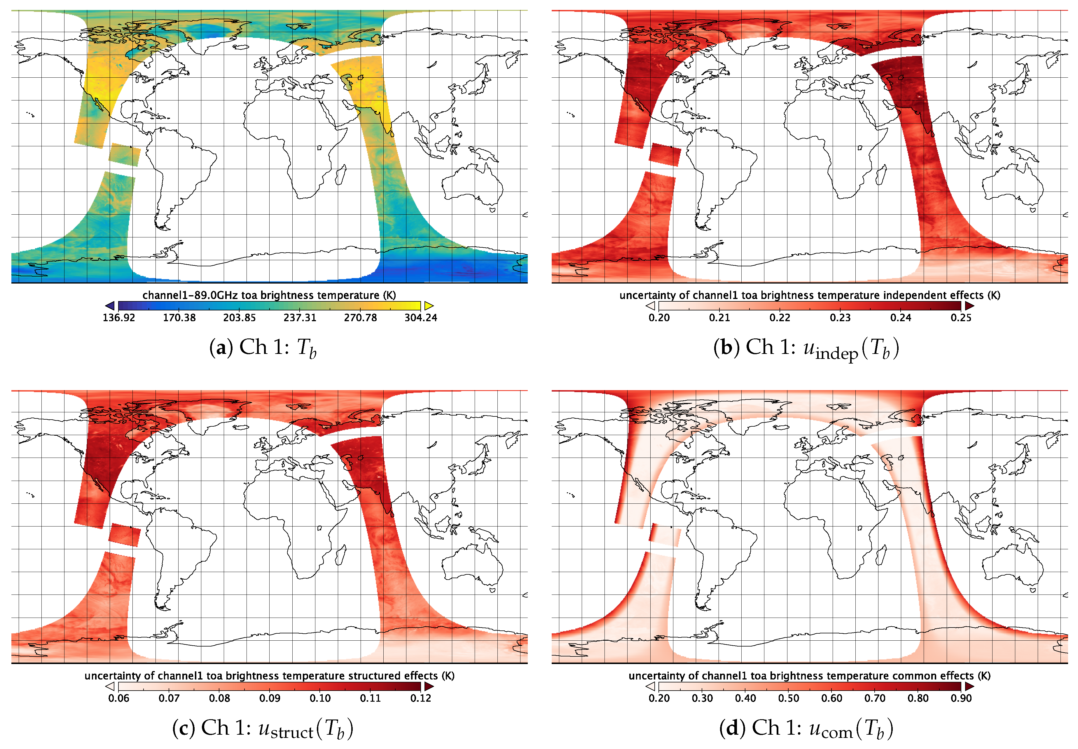
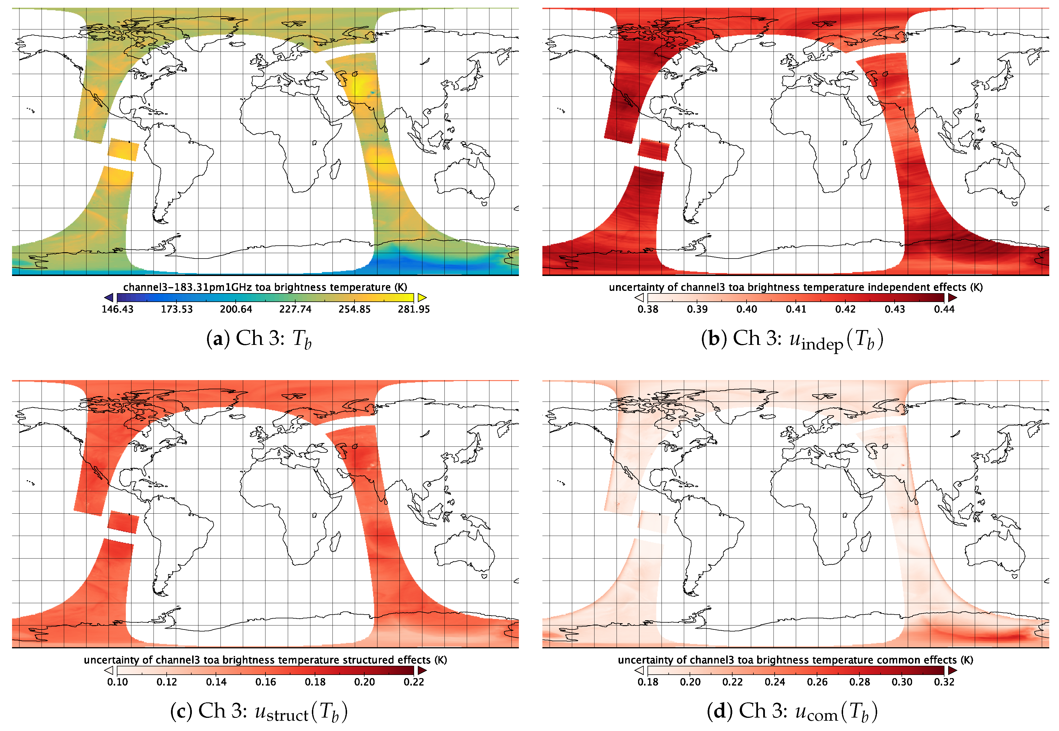
3.2. FCDR Example Contents

In this section, we present example contents from the FCDR processed with the final implementation of the calibration.
The FIDUCEO FCDR is a ready-to-use dataset providing the data of eleven missions of microwave humidity sounders stored in orbital chunks in NetCDF-4 files. In total, the record has a size of 2.2 TB, with 6.8 MB (AMSU-B and MHS) or 0.6 MB (SSMT-2) per file. Each file of the FCDR files contains a single orbit from one equator crossing in a chosen flight direction to the next crossing in the same direction. This equator-to-equator frame makes the files ready-to-use, since it removes the overlap of subsequent orbits. Hence, the tedious handling to remove artefacts due to doubled data is not necessary. Each of these FCDR files contains the calibrated brightness temperature for each channel, its uncertainties categorised by their origin from independent, structured and common effects and concise quality flags conveying helpful information on the usability of the data. Moreover, auxiliary variables are provided in order to maintain traceability back to the original level 1b files.
Figure 3 and Figure 4 show the brightness temperature and its uncertainty for channel 1 and 3 of the example orbit of MHS on Metop-B (start: 6 July 2015 15:47:58, end: 6 July 2015 17:29:18). Note the equator-to-equator frame. The two data gaps seen in this orbit are explained by the quality flags. The quality flags are set during our FCDR processing and provide general information on the quality of the pixels and also on channel-specific issues (see [33] for details on the provided quality information in the FCDR). The first data gap close to South America is due to missing data. The second data gap is due to a moon intrusion in the DSVs, which prohibits the calibration of the affected scan lines. Note also the different ranges and distribution patterns for the uncertainty classes. This is discussed in Section 3.3.

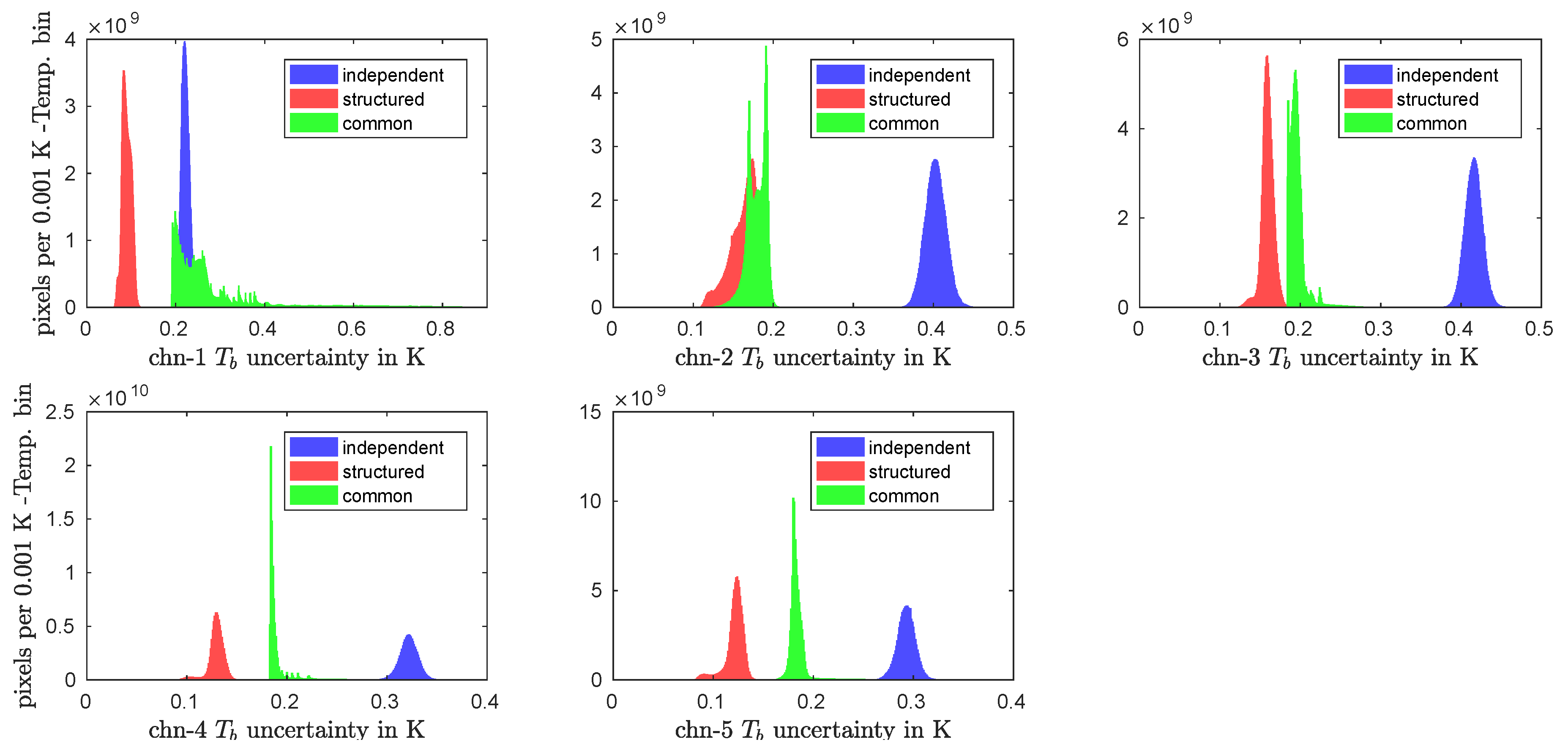
3.3. Assessment of Uncertainties

Because of the lack of detailed uncertainty information in the operational data, a comparison of the uncertainties stored in the new FCDR to other uncertainties is only possible to a limited degree. The operational processor AAPP provides cold and warm NE Δ T per scan line. However, in files processed with AAPP version 7-13, these NE Δ T estimates are only available for MHS while the values for AMSU-B are zero. The warm NE Δ T, obtained from the noise on IWCT counts, can be compared to the uncertainties due to independent effects because the latter are dominated by the noise from Earth counts for which the estimate is obtained from the noise on IWCT counts. Hence, the warm NE Δ T and the uncertainties due to independent effects are related, even though they are not the same. When comparing AAPP warm NE Δ T and uncertainties due to independent effects in the MHS-FCDR, a good correspondence of typical values can be observed for all channels. Being deduced from calibration counts, the warm NE Δ T is also related to the uncertainties due to structured effects. However, their values are smaller than the warm NE Δ T, because the uncertainties due to structured effects take into account the rolling average that reduces noise.
A comparison of the uncertainties due to independent and structured effects to the instrumental specification for NE Δ T is also possible, since both classes of uncertainty are dominated by either the noise on the Earth counts or the noise on the calibration counts, which is also the important aspect in the estimate of NE Δ T. The comparison reveals a fair agreement of deduced uncertainties from the FCDR processing and the reported specified NE Δ T [16]. During periods of erratic instrumental behaviour, such as the later years of AMSU-B on NOAA-15 and on NOAA-16 as well as of MHS on NOAA-19 when the instruments failed the NE Δ T-specifications, the uncertainties of the brightness temperature stored in the FCDR reflect well this erratic behaviour by having increased uncertainties due to independent and structured effects.
The uncertainty due to common effects has no equivalent in the available datasets. Hence, a first analysis of its characteristic distribution over an orbit is especially interesting. Figure 3d and Figure 4d show the uncertainty due to common effects for channel 1 and 3, respectively. Note that the uncertainty introduced by the antenna pattern correction is the strongest contribution for channel 1; the picture of a high uncertainty on the edges of the swath and a low uncertainty around nadir clearly shows the dominance of the antenna pattern correction over the other effects. This dominance arises because of the large operational correction value and the input uncertainty estimates (50% of the operational correction value). Note that channel 3 has a much smaller operational correction. Hence, using the same estimate of 50% leads to a smaller uncertainty than for channel 1. For channel 3, other effects gain influence as can be deduced from the more prominent temperature dependence (compare Figure 4a–d). This temperature dependence of the uncertainty with large uncertainties in cold regions and small uncertainties in warm regions is due to the polarisation correction. This correction also introduces a scan dependence, which leads to smaller uncertainties at the edge of the swath and to larger uncertainties near nadir. This is by construction of the correction formula, which accounts for the polarisation sensitivity of the receiver in connection with the different reflectivities of the rotating mirror for horizontally and vertically polarised radiation. Note that we used 100% of the operational values for the coefficient α as input uncertainty estimate (operational value from NOAA-18 as no other instrument receives a non-zero correction, see above). Nonetheless, it is still the antenna pattern correction that dominates the scan dependence of the uncertainty. At the right edge in flight direction, the uncertainty is increased compared to nadir. At the left edge, the antenna pattern correction has less influence.
A comparison of the three classes of uncertainties is visible in Figure 5, showing histograms of the respective uncertainties for each class for one month of MHS data (MHS on Metop-B, September 2014). The histograms for the three sounding channels resemble each other, although the exact positions of the distributions vary slightly. For channels 1 and 2, the picture is changed as either the independent and common uncertainties, or the structured and common uncertainties overlap. The long tail for the common effects in channel 1 reaching 0.8 K is due to the antenna pattern correction affecting the outermost pixels most strongly. Most of the data, however, have common uncertainties below 0.3 K also for channel 1. Except for channel 1, the independent uncertainties dominate the other classes. From the perspective of a climate scientist, this is encouraging, as the uncertainty due to independent effects can be reduced by averaging procedures used for climate studies. The smaller, common uncertainties cannot be reduced by averaging, hence, their relative importance increases on longer times scales.

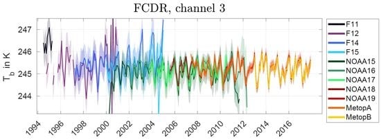
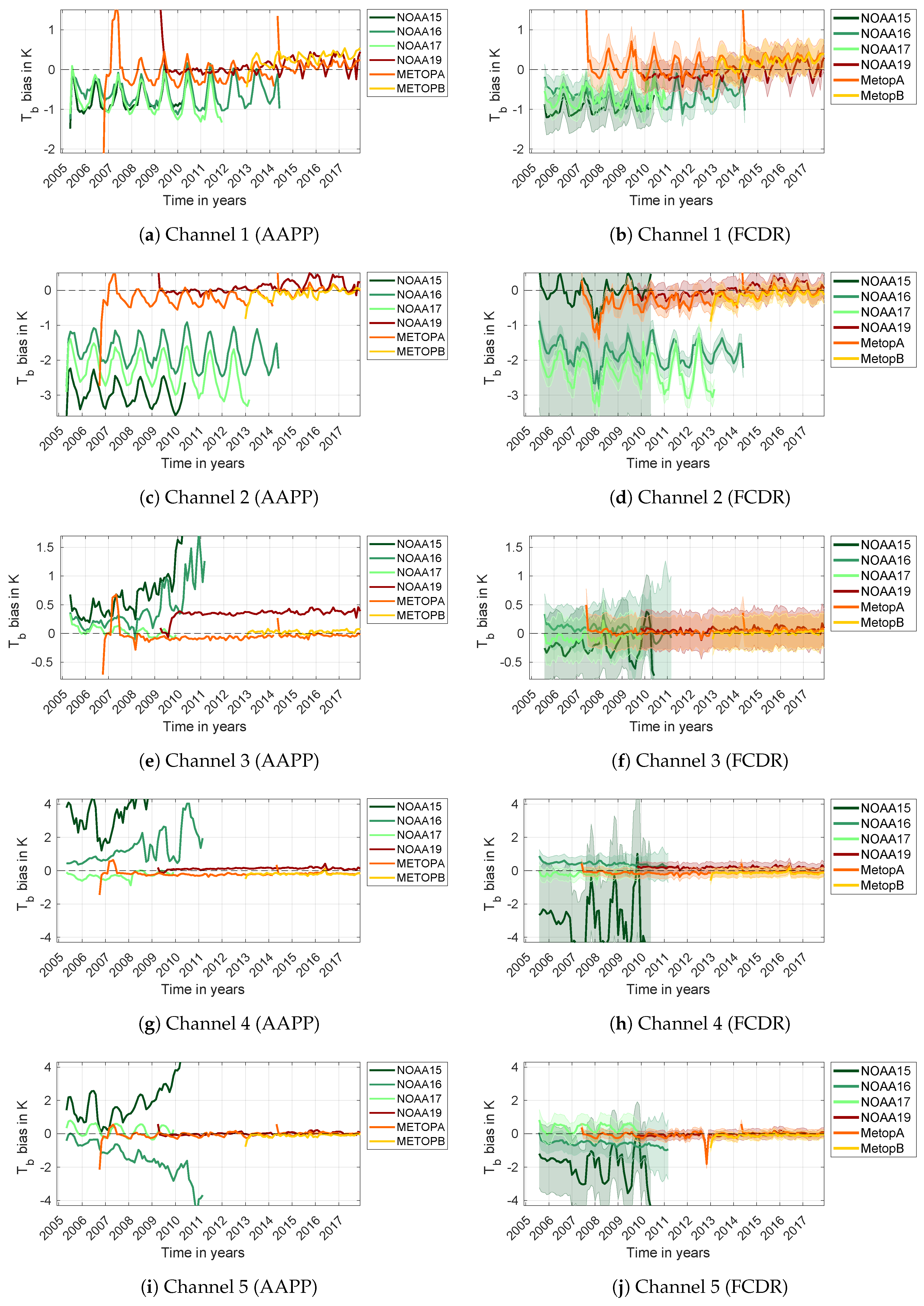
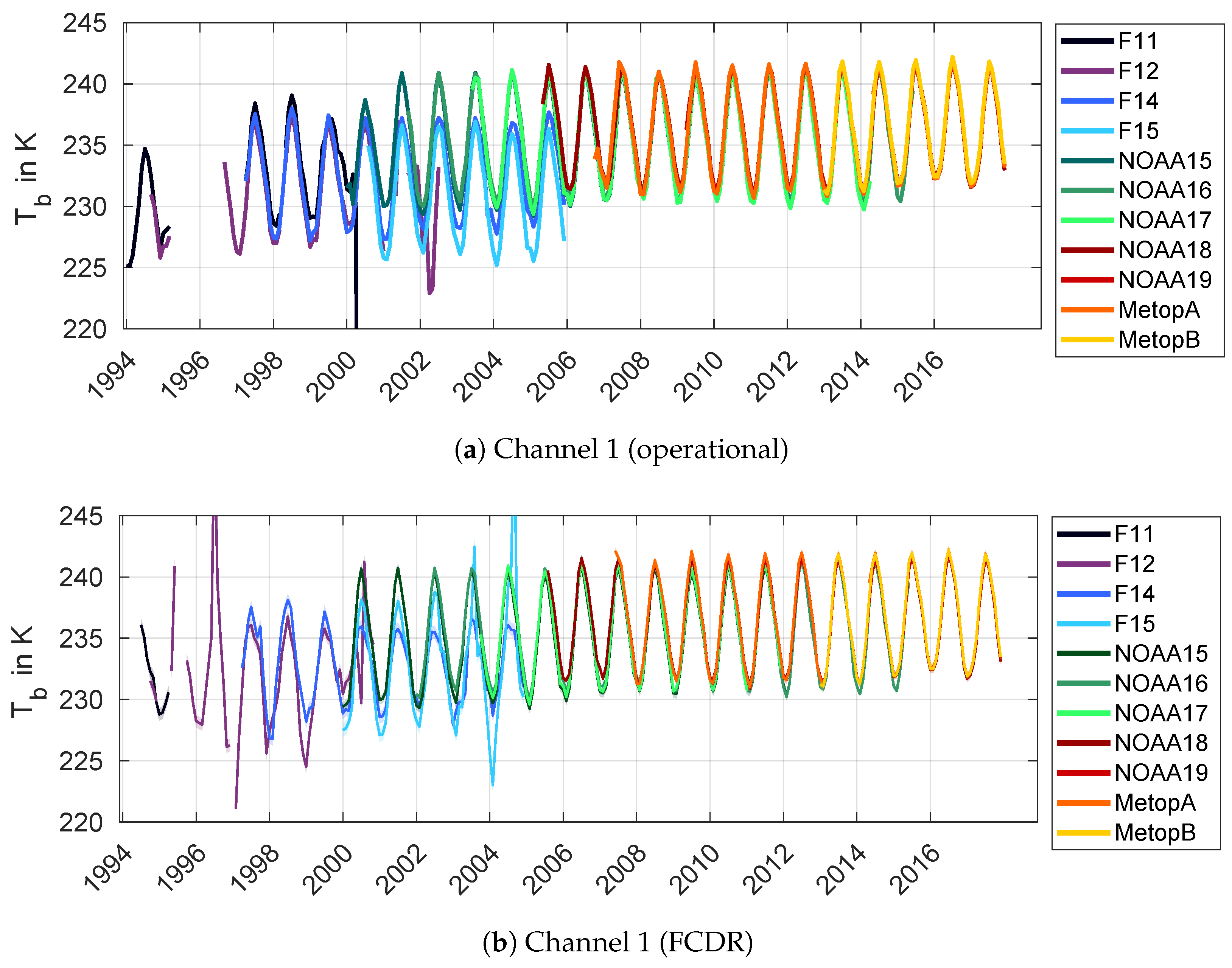
3.4. Inter-Satellite Comparison: Improvements in the FCDR

Applying the improvements explained in Section 2.2.2 to the FCDR processing, we obtained a new FCDR that shows reduced inter-satellite biases. Figure 6 shows the inter-satellite biases in terms of global monthly means, averaged over all scan angles and both ascending and descending passes. The peaks that suddenly appear in the time series (Metop-A, NOAA-18, NOAA-19) may be due to MHS instruments recovering from spin state [39]. The reference is MHS on NOAA-18 because of its long time series and stability. Note also that only AMSU-B and MHS instruments are shown. SSMT-2 cannot be compared to NOAA-18 because of missing overlap. Hence, SSMT-2 is not displayed in Figure 6. The improvement of the SSMT-2 calibration by the strict application of the measurement equation is visible in Figure A1, Figure A2, Figure A3, Figure A4 and Figure A5 showing the time series of the brightness temperature for all instruments and channels for the operational data and the new FCDR data.
Channel 1 is affected by the correction of APC for NOAA-18 and Metop-A. No RFI correction is applied (since the method for deriving the correction does not work for channels strongly affected by the diurnal cycle). There is reasonable agreement between the instruments. Note for example the increasing amplitude of the seasonal cycle for MHS on NOAA-19 as the satellites drift apart. At the same time, the amplitude decreases for Metop-A as NOAA-18 drifts closer to it. The AMSU-B instruments show an offset with respect to the MHS instruments. Note that the channel does not have exactly the same characteristics for AMSU-B and MHS (they differ in bandwidth and location of the two pass bands).
Channel 2 shows very similar results as channel 1. However, AMSU-B on NOAA-15 differs from the other AMSU-Bs. This is because the channel is not RFI-corrected in the FCDR (correction scheme cannot be derived with the applied method). The matching of NOAA-15 to NOAA-18 is not meaningful, since channel 2 differs for MHS and AMSU-B (note the off-set for the other AMSU-Bs).
Channel 3 is affected by the correction of APC for NOAA-18 and Metop-A. Moreover, the RFI-correction scheme for NOAA-15, NOAA-16, NOAA-17 and NOAA-19 affects this channel. A clear improvement in the reduction of the inter-satellite bias is visible. In addition, the individual instrumental stability has improved, especially for NOAA-16. For NOAA-15, the derived RFI-correction scheme is imperfect, because of its strong RFI contamination already in the early years that can be compared to NOAA-18. This imperfection is represented by an increased uncertainty due to common effects.
For channel 4 and 5, similar improvements as for channel 3 can be seen.
Overall, the applied improvements in the parameters of the measurement equation and the correction for RFI contamination have increased the inter-satellite consistency.

4. Discussion

The extensive uncertainty information provided in the new FCDR is novel in the context of microwave humidity sounder data, which lack uncertainty information thus far. The obtained uncertainties stored in the FCDR appear reasonable, although it should be noted that some of them are based on estimates of the uncertainties on the input calibration parameters. These estimates may be rough, but they still provide an impression of the final uncertainty of the brightness temperature that users have to expect. An encouraging result is that the uncertainty due to common effects does not dominate the uncertainty budget, even though we used relatively large estimates for the corresponding input uncertainties. The dominant uncertainty is due to the independent effects whose uncertainty was obtained from a robust computation of the noise by using the Allan deviation.
Using the measurement equation and the same calibration parameter values as AAPP, our FCDR processing chain can reproduce the operational AAPP processed level 1c data. This was the starting point to improve the calibration for AMSU-B and MHS. Applying then the improved measurement equation and the propagation of uncertainties, we generated an uncertainty quantified MW FCDR that shows improved agreement between the individual instruments and increased stability, both aspects needed to construct consistent time series. The applied improvements are the correct assignment of APC and a newly developed RFI-correction scheme for the individual instruments suffering from RFI contamination. Since these improvements reduced the biases distinctly, and, moreover, other effects could be ruled out as source of the biases [40], we have high evidence that we understood the origin of the most important inter-satellite biases.
For SSMT-2, the improvement is based on the strict application of the measurement equation when recalibrating the data from the raw counts.
Further improvements may be achieved when optimising certain calibration parameters in the ongoing FIDUCEO harmonisation effort. Within this harmonisation approach, the optimal values, e.g., for the non-linearity correction, the warm and cold target correction and the polarisation correction, are investigated. The FIDUCEO harmonisation is a novel approach for the inter-calibration of remote-sensing instruments, using recalibration instead of bias-correction. The harmonisation uses SNOs (and off-nadir matches) as the inter-comparison method. The matches form the input for the harmonisation procedure. This procedure is an optimisation approach. It uses the measurement equation and attempts to find optimised values for certain parameters in the measurement equation such that the inter-satellite bias is reduced [41]. In an iterative procedure of harmonisation and analysis of its results, the correct combination of calibration parameters that explains and reduces the biases needs to be found. This is an ongoing effort.
The improvement in the consistency of calibrated MW sounders data that is already achieved opens up the possibility to proceed with investigation of long time series of a derived CDR.
Work with the FCDRs we provide, for example the production of CDRs, is facilitated by a product user guide and a quick start guide. Additional documentation with information about the performance of the microwave sounders is supplied by the FIDUCEO project as well. It deals with properties of the instruments that are not directly relevant to the measurement equation, for example the uniformity of the sounding channels [40] or the full width at half maximum of the beams [42]. Both quantities were determined with innovative methods based on intrusions of the Moon in the DSV.

5. Conclusions

Our new FCDR for microwave humidity sounders addresses three problems of operational data that we intended to solve to make the data usable for climate research.
First, we facilitate the handling of the data by providing the FCDR in ready-to-use NetCDF files. Each of these files covers one orbit reaching from one equator and crossing to the next in the same flight direction. This equator-to-equator frame removes all doubled data and hence prevents the appearance of corresponding sampling artefacts. The FCDR contains concise quality information on pixel level and maintains the traceability back to the original level 1b data.
Second, the FCDR provides extensive pixel-level uncertainty information, considering the correlation behaviour of the underlying errors.
Third, we have strong evidence that we understood the origin of the most important inter-satellite biases. By applying corresponding corrections, we were able to produce an FCDR for MW sounders of distinctly improved consistency. The sounding channels show very good agreement between the instruments and offer the possibility for using the FCDR for the production of the higher level CDR.
Datasets will be available from the CEDA archive http://archive.ceda.ac.uk/ access via http://www.ceda.ac.uk.

Author Contributions

Conceptualization, S.A.B.; Formal analysis, I.H. and M.B.; Investigation, I.H., M.B., T.L. and M.P.; Software, I.H., M.B., T.L. and M.P.; Validation, I.H., M.B., T.L. and M.P.; Writing—original draft, I.H.; and Writing—review and editing, S.A.B. and V.O.J.

Funding

This research was performed within the project Fidelity and Uncertainty in Climate data records from Earth Observation (FIDUCEO, www.fiduceo.eu), which received funding from the European Union’s Horizon 2020 Programme for Research and Innovation, under Grant Agreement no. 638822.

Acknowledgments

We would like to thank Emma Woolliams for discussions on error correlation structures and valuable comments on the manuscript. We also thank Oliver Lemke for his technical support. For providing the level 1b data, we thank NOAA CLASS.

Conflicts of Interest

The authors declare no conflict of interest. The founding sponsors had no role in the design of the study; in the collection, analyses, or interpretation of data; in the writing of the manuscript, and in the decision to publish the results.

Abbreviations

The following abbreviations are used in this manuscript:
AAPPATOVS and AVHRR Pre-processing Package
AMSU-BAdvanced Microwave Sounding Unit -B
APCantenna pattern correction
ATOVSAdvanced TIROS-N Operational Vertical Sounder
AVHRRAdvanced Very High Resolution Radiometer
CDRclimate data record
DMSPDefense Meteorological Satellite Program
DSVdeep space view
ECVessential climate variable
EUMETSATEuropean Organisation for the Exploitation of Meteorological Satellites
FCDRfundamental climate data record
FIDUCEOFidelity and uncertainty in climate data records from Earth observation
IWCTinternal warm calibration target
LECTlocal equator crossing time
MHSMicrowave Humidity Sounder
MWmicrowave
NE Δ TNoise equivalent differential temperature
NetCDFNetwork Common Data Format
NOAA CLASSNOAA—Comprehensive Large Array-data Stewardship System
NOAA NCEINOAA—National Centers for Environmental Information
NWPnumerical weather prediction
RFIradio frequency interference
SNOsimultaneous nadir overpass
SSM/ISpecial Sensor Microwave Imager
SSMT-2Special Sensor Microwave Water Vapor Profiler
UTHupper tropospheric humidity

Appendix A

Figure A1. Comparing the time series of brightness temperature in channel 1 for all MW instruments in (a) operational data (NGDC for SSMT-2 and AAPP processed data for AMSU-B and MHS) and (b) FCDR data as function of time. The FCDR provides more consistent and stable time series due to improved calibration. For the FCDR, the shaded regions denote the uncertainty due to common effects (hardly visible for channel 1 on this scale). There is no corresponding uncertainty estimate on the operational data.
Remotesensing 11 00548 g0a1
Figure A2. The same as Figure A1 but for channel 2. Note the uncertainty for NOAA-15 due to uncorrected RFI.
Remotesensing 11 00548 g0a2
Figure A3. The same as Figure A1 but for channel 3. The instruments agree within the uncertainties. A distinct improvement is also achieved for SSMT2.
Remotesensing 11 00548 g0a3
Figure A4. The same as Figure A1 but for channel 4. Note that NOAA-15 still shows differences with respect to the other instruments. This is due to the imperfect RFI correction.
Remotesensing 11 00548 g0a4
Figure A5. The same as Figure A1 but for channel 5.
Remotesensing 11 00548 g0a5

References

  1. John, V.O.; Allan, R.P.; Bell, B.; Buehler, S.A.; Kottayil, A. Assessment of inter-calibration methods for satellite microwave humidity sounders. J. Geophys. Res. 2013, 118, 4906–4918. [Google Scholar] [CrossRef]
  2. Hanlon, H.; Ingram, W. Algorithm Theoretical Basis Document, Fundamental Climate Data Record of Microwave Brightness Temperatures, CF-26/27/28, version 1.0; Technical Report SAF/CM/UKMO/ATBD/FCDR_MWAVE; Satellite Application Facility on Climate Monitoring (CM SAF), 2016. Available online: www.cmsaf.eu (accessed on 6 March 2019).
  3. Ferraro, R. AMSU-B/MHS Brightness Temperature—Climate Algorithm Theoretical Basis Document, NOAA Climate Data Record Program CDRP-ATBD-0801 Rev. 1; Technical report; NOAA STAR: College Park, MD, USA, 2016.
  4. Zou, C.Z.; Goldberg, M.D.; Cheng, Z.; Grody, N.C.; Sullivan, J.T.; Tarpley, D. Recalibration of microwave sounding unit for climate studies using simultaneous nadir overpasses. J. Geophys. Res. 2006, 111. [Google Scholar] [CrossRef] [Green Version]
  5. Moradi, I.; Beauchamp, J.; Ferraro, R. Radiometric correction of observations from microwave humidity sounders. Atmos. Meas. Tech. 2018, 11, 6617–6626. [Google Scholar] [CrossRef]
  6. Chung, E.S.; Soden, B.J.; John, V.O. Intercalibrating microwave satellite observations for monitoring long-term variations in upper and mid-tropospheric water vapor. J. Atmos. Ocean. Technol. 2013, 30, 2303–2319. [Google Scholar] [CrossRef]
  7. Shi, L.; Bates, J.J. Three decades of intersatellite-calibrated High-Resolution Infrared Radiation Sounder upper tropospheric water vapor. J. Geophys. Res. 2011, 116. [Google Scholar] [CrossRef] [Green Version]
  8. Chung, E.S.; Soden, B.J.; Huang, X.; Shi, L.; John, V.O. An assessment of the consistency between satellite measurements of upper tropospheric water vapor. J. Geophys. Res. 2016, 121, 2874–2887. [Google Scholar] [CrossRef]
  9. Wentz, F.J.; Mears, C.A.; Program, N.C. NOAA Climate Data Record (CDR) of SSM/I and SSMIS Microwave Brightness Temperatures, RSS Version 7; NOAA National Centers for Environmental Information: Silver Spring, MD, USA, 2013. [CrossRef]
  10. Kummerow, C.D.; Berg, W.K.; Sapiano, M.R.P.; Program, N.C. NOAA Climate Data Record (CDR) of SSM/I and SSMIS Microwave Brightness Temperatures, CSU Version 1; NOAA National Climatic Data Center: Silver Spring, MD, USA, 2013.
  11. Berg, W.; Kroodsma, R.; Kummerow, C.D.; McKague, D.S. Fundamental Climate Data Records of Microwave Brightness Temperatures. Remote Sens. 2018, 10, 1306. [Google Scholar] [CrossRef]
  12. Fennig, K.; Schröder, M.; Hollmann, R. Fundamental Climate Data Record of Microwave Imager Radiances; Satellite Application Facility on Climate Monitoring (CM SAF), 2017, 3rd ed. Available online: www.cmsaf.eu (accessed on 3 March 2019).
  13. Zou, C.Z.; Wang, W. Intersatellite calibration of AMSU-A observations for weather and climate applications. J. Geophys. Res. 2011, 116. [Google Scholar] [CrossRef] [Green Version]
  14. Mo, T. Inter-satellite calibration of the NOAA AMSU-A measurements over tropical oceans. Remote Sens. Environ. 2014, 149, 205–212. [Google Scholar] [CrossRef]
  15. Chander, G. Overview of Intercalibration of Satellite Instruments. IEEE Trans. Geosci. Remote Sens. 2013, 51, 1056–1080. [Google Scholar] [CrossRef]
  16. NOAA. NOAA KLM User’s Guide with NOAA-N, -N’ Supplement; Technical Report; National Oceanic and Atmospheric Administration, National Environmental Satellite, Data, and Information Service, National Climatic Data Center, Remote Sensing and Applications Division, 2009. Available online: https://www.noaa.gov/ (accessed on 6 March 2019).
  17. Kobayashi, S.; Poli, P.; John, V.O. Characterisation of Special Sensor Microwave Water Vapor Profiler (SSM/T-2) radiances using radiative transfer simulations from global atmospheric reanalyses. Adv. Space Res. 2016, 59, 917–935. [Google Scholar] [CrossRef]
  18. Labrot, T.; Lavanant, L.; Whyte, K.; Atkinson, N.; Brunel, P. AAPP Documentation Scientific Description, Version 6.0, Document NWPSAF-MF-UD-001; Technical Report. NWP SAF, Satellite Application Facility for Numerical Weather Prediction, 2006. Available online: https://www.nwpsaf.eu/site/ (accessed on 6 March 2019).
  19. Woolliams, E.; Mittaz, J.; Merchant, C.J.; Harris, P. D2.2a: Principles Behind the FCDR Effects Tables; Technical Report. National Physical Laboratory and University of Reading, 2017. Available online: www.npl.co.uk/ (accessed on 6 March 2019).
  20. Saunders, R.W.; Hewison, T.J.; Stringer, S.J.; Atkinson, N.C. The Radiometric Characterization of AMSU-B. IEEE Trans. Microw. Theory Tech. 1995, 43, 760–771. [Google Scholar] [CrossRef]
  21. Hewison, T.J.; Saunders, R. Measurements of the AMSU-B Antenna Pattern. IEEE Trans. Geosci. Remote Sens. 1996, 34, 405–412. [Google Scholar] [CrossRef]
  22. Klaes, D.; Ackermann, J. Techniques and Processes for Pre-Launch Characterisation of New Instruments; Technical Report. EUMETSAT, 2014. Available online: https://www.eumetsat.int/ (accessed on 6 March 2019).
  23. Atkinson, N.C.; McLellan, S. Initial evaluation of AMSU-B in-orbit data. Proce. SPIE Int. Soc. Opt. Eng. 1998, 3503, 276–287. [Google Scholar] [CrossRef]
  24. Atkinson, N.C. Performance of AMSU-B Flight Model 2 (FM2) During NOAA-L Post Launch Orbital Verification Tests, AMB112; Technical Report; Remote Sensing Instrumentation, Met Office: Exeter, UK, 2000.
  25. Atkinson, N.C. Performance of AMSU-B Flight Model 3 (FM3) During NOAA-M Post Launch Orbital Verification Tests, AMB113; Technical Report; Remote Sensing Instrumentation, Met Office: Exeter, UK, 2002.
  26. Hewison, T.J. A Thermal Model of Black Body Targets; Met Office (RS) Working Paper No. 29, August 1991; Met Office: Exeter, UK; Farnborough, UK, 1991; 12p.
  27. JPSS ATMS SDR Science Team. Joint Polar Satellite System (JPSS) Advanced Technology Microwave Sounder (ATMS) SDR Calibration Algorithm Theoretical Basis Document (ATBD); Technical Report; NOAA Center for Sattelite Application and Research: Silver Spring, MD, USA, 2013.
  28. Burgdorf, M.; Hans, I.; Prange, M.; Mittaz, J.; Woolliams, E. D2.2 Microwave: Report on the MW FCDR Uncertainty; Technical Report; Universität Hamburg, National Physical Laboratory: Hamburg, Germany, 2017. [Google Scholar]
  29. Khan, S.; Shaw, G. PFM Radiometric Calibration Test Report, MHS-TR-JA281-MMP; Technical Report; MATRA MARCONI SPACE UK Limited: Paris, France, 1999. [Google Scholar]
  30. Atkinson, N.C. Calibration, monitoring and validation of AMSU-B. Adv. Space Res. 2001, 28, 117–126. [Google Scholar] [CrossRef]
  31. John, V.O.; Holl, G.; Atkinson, N.; Buehler, S.A. Monitoring scan asymmetry of microwave humidity sounding channels using simultaneous all angle collocations (SAACs). J. Geophys. Res. 2013, 118, 1536–1545. [Google Scholar] [CrossRef] [Green Version]
  32. Hans, I.; Burgdorf, M.; Buehler, S.A. On-board radio frequency interference as origin of inter-satellite biases for microwave humidity sounders. Unpublished, in preparation.
  33. Hans, I.; Burgdorf, M.; Woolliams, E. Product User Guide—Microwave FCDR Release 4.1; Techreport; Universität Hamburg and National Physical Laboratory: Hamburg, Germany, 2019. [Google Scholar]
  34. Fixsen, D.J. The temperature of the cosmic microwave background. Astrophys. J. 2009, 707. [Google Scholar] [CrossRef]
  35. Joint Committee for Guides in Metrology (JCGM). Evaluation of Measurement Data—Guide to the Expression Of Uncertainty in Measurement (GUM) JCGM 100:2008. 1995. Available online: http://www.bipm.org/en/publications/guides (accessed on 15 July 2018).
  36. Hans, I.; Burgdorf, M.; John, V.O.; Mittaz, J.; Buehler, S.A. Noise performance of microwave humidity sounders over their life time. Atmos. Meas. Tech. 2017, 10, 4927–4945. [Google Scholar] [CrossRef]
  37. Tian, M.; Zou, X.; Weng, F. Use of Allan Deviation for Characterizing Satellite Microwave Sounder Noise Equivalent Differential Temperature (NEDT). IEEE Geosci. Remote Sens. Lett. 2015, 12, 2477–2480. [Google Scholar] [CrossRef]
  38. Merchant, C.J.; Woolliams, E.; Mittaz, J. Uncertainty and Error Correlation Quantification for FIDUCEO easyFCDR Products: Mathematical Recipes, v0.9; Technical Report; University of Reading, National Physical Laboratory: Reading, Berkshire, UK, 2017. [Google Scholar]
  39. NOAA-OSPO. POES Operational Status Webpage. 2015. Available online: http://www.ospo.noaa.gov/Operations/POES/status.html (accessed on 14 December 2017).
  40. Burgdorf, M.; Hans, I.; Prange, M.; Lang, T.; Buehler, S.A. Inter-channel uniformity of a microwave sounder in space. Atmos. Meas. Tech. 2018, 11. [Google Scholar] [CrossRef]
  41. Giering, R.; Quast, R.; Mittaz, J.; Hunt, S.; Harris, P.; Wooliams, E. Harmonisation of fundamental satellite data records. Remote Sens. 2019. in preparation. [Google Scholar]
  42. Burgdorf, M. Disk-Integrated Lunar Brightness Temperatures Between 89 and 190 GHz. Adv. Astron. 2019. submitted. [Google Scholar]
Figure 1. The full MW measurement equation. L ˜ MIWCT , L ˜ MS and L ˜ ME denote the radiances as they are recorded by the instrument, i.e., including additional radiation not originating from the IWCT, space or Earth, respectively. Any uncertainty component is denoted by u ( ) . w k denotes the weight of individual PRT measurements in the overall average (green box). B denotes the Planck function. The light green box labelled harmonisation relates to the ongoing effort of further improvement of certain calibration parameters included in a vector a (see Section 4). Graphical design: Jonathan Cherry and Emma Woolliams.
Remotesensing 11 00548 g001
Figure 2. Difference in brightness temperature (channel 3) of FIDUCEO and AAPP processing for an example orbit of Metop-A: (a) for initial implementation that imitates AAPP; and (b) for final implementation with improvements in the calibration to reduce inter-satellite biases.
Remotesensing 11 00548 g002
Figure 3. Channel 1: Brightness temperature and its uncertainties (example orbit of MHS on Metop-B).
Remotesensing 11 00548 g003
Figure 4. Channel 3: Brightness temperature and its uncertainties (example orbit of MHS on Metop-B).
Remotesensing 11 00548 g004
Figure 5. Histogram of the three classes of uncertainties for September 2014, MHS on Metop-B, all channels.
Remotesensing 11 00548 g005
Figure 6. Comparing inter-satellite biases of MHS and AMSU-B instruments against MHS on NOAA-18 in operational AAPP data (left) and FCDR data (right) as function of time. The FCDR provides more consistent and stable time series due to improved calibration. The instruments agree within the uncertainties (only uncertainties due to common effects displayed here). Note that channel 2 differs slightly in frequency for MHS and AMSU-B and therefore is not expected to match completely.
Remotesensing 11 00548 g006
Table 1. Launch and end of life dates and periods of available FCDR data.
Instrument and SatelliteLaunchedEnd of LifeFCDR start dateFCDR End Date
SSMT-2 F1128 November 19917 August 20005 July 19942 April 1995
SSMT-2 F1229 August 199413 October 200813 October 19948 January 2001
SSMT-2 F144 April 1994201528 April 199710 January 2005
SSMT-2 F1512 December 1999201524 January 20002 January 2005
AMSU-B NOAA-1513 May 199828 March 20111 January 199928 March 2011
AMSU-B NOAA-1621 September 20009 June 201420 March 200130 April 2014
AMSU-B NOAA-1724 June 200210 April 201315 October 200210 April 2013
MHS NOAA-1820 May 2005≥201830 August 200531 December 2017
MHS NOAA-196 February 2009≥20181 November 200931 December 2017
MHS Metop-A19 October 2006≥20181 June 200731 December 2017
MHS Metop-B17 September 2012≥201829 January 201331 December 2017
Table 2. The basic instrumental characteristics of SSMT-2, AMSU-B and MHS. Note that all channels have two side bands, although rarely indicated for MHS channels 1, 2 and 5 where the side bands are very close to each other. The values for the NE Δ T stem from the specifications for SSMT-2, from NOAA-15 for AMSU-B and NOAA-18 for MHS.
Channel (in This Article)Orig. ChannelFrequency in GHzTotal Bandwidth in GHzPre-Launch NE Δ T in K
1491.655 ± 1.25030.6
25150.00 ± 1.2530.6
SSMT-232183.31 ± 1.0010.8
41183.31 ± 3.0020.6
53183.31 ± 7.0030.6
11689.0 ± 0.920.37
217150.0 ± 0.920.84
AMSU-B318183.31 ± 1.011.06
419183.31 ± 3.020.70
520183.31 ± 7.040.60
1H189.02.80.22
2H2157.02.80.34
MHS3H3183.31 ± 1.010.51
4H4183.31 ± 3.020.40
5H5190.312.20.46

