Seeking Optimal GNSS Radio Occultation Constellations Using Evolutionary Algorithms


1
School of Geodesy and Geomatics, Wuhan University, 129 Luoyu Road, Wuhan 430079, China
2
Collaborative Innovation Center for Geospatial Technology, 129 Luoyu Road, Wuhan 430079, China
3
Key Laboratory of Geospace Environment and Geodesy, Ministry of Education, 129 Luoyu Road, Wuhan 430079, China
4
German Research Centre for Geosciences GFZ, 14473 Potsdam, Germany
5
Institute of Geodesy and Geoinformation Science, Technische Universität, 10623 Berlin, Germany
*
Author to whom correspondence should be addressed.
Remote Sens. 2019, 11(5), 571; https://0-doi-org.brum.beds.ac.uk/10.3390/rs11050571
Submission received: 24 January 2019
/
Revised: 26 February 2019
/
Accepted: 4 March 2019
/
Published: 8 March 2019
(This article belongs to the Special Issue Selected Papers from IGL-1 2018 — First International Workshop on Innovating GNSS and LEO Occultations & Reflections for Weather, Climate and Space Weather)
Abstract
:Given the great achievements of the Constellation Observing System for Meteorology, Ionosphere, and Climate (COSMIC) mission in providing huge amount of GPS radio occultation (RO) data for weather forecasting, climate research, and ionosphere monitoring, further Global Navigation Satellite System (GNSS) RO missions are being followingly planned. Higher spatial and also temporal sampling rates of RO observations, achievable with higher number of GNSS/receiver satellites or optimization of the Low Earth Orbit (LEO) constellation, are being studied by high number of researches. The objective of this study is to design GNSS RO missions which provide multi-GNSS RO events (ROEs) with the optimal performance over the globe. The navigation signals from GPS, GLONASS, BDS, Galileo, and QZSS are exploited and two constellation patterns, the 2D-lattice flower constellation (2D-LFC) and the 3D-lattice flower constellation (3D-LFC), are used to develop the LEO constellations. To be more specific, two evolutionary algorithms, including the genetic algorithm (GA) and the particle swarm optimization (PSO) algorithm, are used for searching the optimal constellation parameters. The fitness function of the evolutionary algorithms takes into account the spatio-temporal sampling rate. The optimal RO constellations are obtained for which consisting of 6–12 LEO satellites. The optimality of the LEO constellations is evaluated in terms of the number of global ROEs observed during 24 h and the coefficient value of variation (COV) representing the uniformity of the point-to-point distributions of ROEs. It is found that for a certain number of LEO satellites, the PSO algorithm generally performs better than the GA, and the optimal 2D-LFC generally outperforms the optimal 3D-LFC with respect to the uniformity of the spatial and temporal distributions of ROEs.
1. Introduction
Satellite constellation design is an essential sector of designing spacecraft missions such as global navigation, communication, remote sensing, and Earth and space observation. These satellite missions may consist of multiple spacecrafts which operate simultaneously in order to meet the optimal performance of the system and reduce the mission costs [1].
The radio occultation (RO) technique was originally used to study the atmosphere and ionosphere of Mars [2]. The idea of using GPS RO technology to study the Earth’s atmosphere was pioneered by the GPS/Meteorology (GPS/MET) experiment launched in 1995 [3,4]. Since then, large amounts of vertical profiles of atmospheric and ionospheric parameters have been obtained by following satellite missions, including the CHAllenging Minisatellite Payload (CHAMP) [5], the Constellation Observing System for Meteorology, Ionosphere and Climate (COSMIC) [6], the Meteorological operational satellite-A (MetOp-A) [7], MetOp-B [8], and FengYun-3C [9]. For RO missions with single LEO satellite such as GPS/MET and CHAMP, the number of daily RO events (ROEs) and the corresponding spatial and temporal resolution of RO data were limited. COSMIC, the first operational GPS RO constellation with six satellites, has observed 1000–2500 ROEs per day at the early stages of its operation [10,11]. The resultant data contribute significantly to weather forecasting [12], the global climate change [13], space weather monitoring [6], and ionospheric climate studies [14]. Due to the great success of the COSMIC mission, the follow-on mission COSMIC-2 is initially designed with six low-inclination-angle and six high-inclination-angle orbit satellites. Although the launch of six high-inclination-angle orbit satellites of COSMIC-2 was finally canceled due to budget constraints, it is likely that an alternative source can be obtained from high latitude constellations provided by commercial companies [15].
On the other hand, the number of navigation satellites whose signal can be used for the RO observation has increased continuously in recent years. Over the past decade, navigation satellite systems are being developed and emerging, such as the Chinese BeiDou navigation system (BDS), Galileo and Japanese Quasi-Zenith Satellite System (QZSS) and will bring unique opportunities and challenges for the Global Navigation Satellite System (GNSS) RO technique, in addition to the fully operational GPS and GLONASS. With the increased number of available navigation satellites, the use of multiple GNSS signals is an opportunity for better sounding of the atmosphere [16]. The new generation of GNSS RO missions is normally equipped with multi-GNSS RO receivers. Each of the six COSMIC-2 satellites is equipped with a GNSS RO receiver, which will receive navigation signals from both GPS and GLONASS [17]. The GNSS occultation sounder (GNOS) instrument onboard FY-3C and FY-3D satellites can receive signals from Beidou Navigation Satellite System (BDS) and GPS [18,19]. The new instrument, named GNOS-II, onboard FY-3E satellite is capable of tracking GNSS signals from GPS, BDS, and Galileo [20].
Better temporal and spatial distribution of ROEs, important components of designing a GNSS RO system, is a motivation for extensive researches. Mousa et al. [21] used the variable separation approach to seek the best practical orbital parameters of the LEO satellite for a tropical GPS RO mission, and the performance of the orbit design is evaluated with the number of ROEs and their longitudinal and latitudinal distributions. Xu et al. [22] analyzed the impact of LEO orbit parameters on the number and global distribution of RO events. Moreover, the impacts of the orbit inclination angles of LEO satellites on the performance of the COSMIC and COSMIC-2 was investigated by Chern et al. [23]. For the first time, Juang et al. [24] used a genetic algorithm (GA) for the optimal design of a walker constellation composed of 12 satellites in a multi-GNSS RO mission. The fitness function of the GA applied in Reference [24] is established on the basis of the minimum number of 24 h ROEs over each 4.5° × 4.5° longitude–latitude grid cell and the temporal distribution of the ROEs is not considered. Lee and Mortari [25] also applied GA to optimize the 2D-lattice flower constellations composed of 12 satellites for a LEO-LEO RO mission, with the purpose of maximizing the odds at which pairs of satellites can see each other through the atmosphere (active or observation time). Asgarimehr and Hossainali [26] further used GA to optimize the 2D-lattice flower constellation (2D-LFC) and 3D-lattice flower constellation (3D-LFC) composed of 6 LEO satellites for GPS RO observations over Asia and the Pacific region, and the performances of the optimized constellations for RO observation are even superior to COSMIC over the target region. They devised the fitness function based on the concept of a Voronoi diagram, which evaluates the spatio-temporal distribution of ROEs. In these previous studies which use the evolutionary algorithms to optimize the RO constellation [24,25,26], a GA is generally applied. While in the design of optimal satellite constellations for different kinds of applications, another evolutionary algorithm, the particle swarm optimization (PSO) algorithm, is also widely used and it has been documented that a PSO performs even better than a GA [27,28].
In this study, the navigation signals from all the five available Global Navigation Satellite Systems (GNSS) (i.e., GPS, GLONASS, BDS, GALILEO, and QZSS) are fully exploited for the first time and two constellation patterns, the 2D-LFC and 3D-LFC, are adopted to develop the optimal constellations composed of 6–12 LEO satellites for GNSS RO observations over the globe. Considering that the optimization algorithms may result in different performance levels of the eventual constellation [27], both GA and PSO are applied to search for the optimal configuration of the constellation for GNSS RO observations. The fitness function of the evolutionary algorithms is established based on the concept of spatio-temporal point process. Both the spatial and the temporal distributions of ROEs are taken into consideration evaluating the optimality of the resultant constellation.
In what follows, we outline how this is done. Section 2 describes the principles and the methods used in the optimization process and the simulations. In Section 3, the optimal constellation configurations are presented and are evaluated. The comparisons of the methods and results with related researches are discussed in Section 4, and some conclusions are reached in Section 5.
2. Principles and Methods
For cost consideration, we limited the total number of LEO satellites to less than or equal to 12 [24]. Considering that COSMIC is a six-satellite constellation, the minimum number of LEO satellites is set at 6. Hence, the optimal constellations are obtained by a varying number of LEO satellites between 6 and 12. The two LEO constellation patterns, the two evolutionary algorithms with their implemented fitness function, the simulation scenario, and the criteria to evaluate the point-to-point uniformity of the ROE distributions are presented in this section.
2.1. LEO Constellation Patterns
To design the LEO satellite constellation for a spacecraft mission, two walker constellation patterns, walker delta and walker star constellation, are generally chosen [29,30]. Two types of lattice flower constellations, 2D-LFC and 3D-LFC, can also be considered as walker constellations [31,32]. Here the LEO constellation patterns of 2D-LFC and 3D-LFC are taken into consideration. Considering that the uniformity and the symmetry of the constellation can be affected by elliptical orbits in 2D-LFC [26], only circular orbits are considered for optimizations based on this pattern, while 3D-LFC is applied for constellation pattern of elliptical orbits.
2.1.1. 2D-LFC
A 2D-LFC is defined with three integer parameters and six continuous ones [31]. The three integer parameters are the number of inertial orbits (), the number of satellites per orbit () and the phasing parameter (), which satisfies and governs the phasing distribution of the satellites in the constellation. The six continuous parameters are the orbit altitude (a), the eccentricity (e), the inclination (i), the argument of perigee (w), the longitude of the ascending node (), and the initial mean anomaly of the first satellite of the constellation (). In particular, the distribution of the satellites in a 2D-LFC corresponds to a lattice in space, where the mean anomaly (M) and the right ascension of the ascending node () of all the satellites of the constellation are uniformly distributed in orbits. The constellation configuration for a 2D-LFC is expressed as follows [31]:
where , ; ; , , among which and denote the longitude of the ascending node and the mean anomaly of the j-th satellite on the i-th orbital plane, respectively. and are calculated with Equation (1), based on which and can be obtained accordingly with the given and .
In the simulation, circular orbits need to be applied to ensure the uniform and symmetric distribution of the LEO satellites in the 2D-LFC [31], which means that the eccentricity of all the satellites are set to be zero. Some constraints are applied on the variation range of the design parameters for the LEO constellation to avoid unrealistic solutions. The variation ranges of the constellation parameters for the 2D-LFC are listed in Table 1. Due to the regular pattern of the 2D-LFC, it is possible that the satellites will collide in circular orbits. Hence, to avoid the collision of satellites within the 2D-LFC, the constraint on the minimum approach distance between any two satellites is considered, as explained in Reference [33]. In the optimization process, the fitness value will be set to the minimum when this constraint is not satisfied.
2.1.2. 3D-LFC
A 3D-LFC is defined by six integer parameters and six continuous ones [32]. Two of the six integer parameters, and , are of the same meanings as those defined for 2D-LFC, and the other four integer parameters include the number of unique orbits (with different arguments of perigee) on each plane () and the three phasing parameters (). Each satellite has the same semi-major axis, eccentricity, and inclination. This results in the most important characteristic of a 3D-LFC, which is the constellation symmetry. In other words, all the satellites in the elliptical orbits are distributed uniformly. The expression to obtain the orbital elements of the satellites in a 3D-LFC reads [32]:
where , , , , , and ; , and are the values of , and of the j-th satellite on the k-th orbits of the i-th orbital plane with respect to the reference satellite, respectively. The variation ranges of the constellation parameters for the 3D-LFC in the simulation are listed in Table 2.
2.2. An Overview of the Evolutionary Algorithms
When seeking the optimal LEO configuration as a GNSS RO mission, the direct way is the exhaustive search method. Considering the large size of search space for both 2D-LFC and 3D-LFC, an exhaustive search is computationally unfeasible. Additionally, when seeking the Geometric Dilution Of Precision (GDOP)-optimal flower constellations for globe coverage problems, the optimized constellation configuration found is responsive to the optimization algorithm used, and the solutions obtained by two evolutionary algorithms, GA and PSO, are generally better than those obtained by an exhaustive algorithm [27]. Therefore, both of these two evolutionary algorithms are used here to seek the best constellation parameters for 2D-LFC and 3D-LFC with the optimal GNSS RO performance over the globe.
2.2.1. Genetic Algorithm (GA)
GA is a robust technique based on natural biological evolution which has proven to be an efficient method to optimize satellite constellations [34]. With the principle of “survival of the fittest”, the GA is initialized with a population of candidate individuals. These individuals are represented by chromosomes that perform selection, crossover, and mutation to form the next generation of the population. In each generation, the fitness of every chromosome is evaluated with the fitness function, and the evolution process terminates when a maximum number of generations or a satisfactory fitness level has been reached. See [35,36] for details.
To deploy GA, 30 individuals, i.e., 30 different constellation configurations of 2D-LFC and 3D-LFC, are created randomly as the initial population. Each individual is represented in the form of chromosomes with the same length in the GA process. It is essential that the constellation parameters of the 2D-LFC and 3D-LFC are encoded as chromosomes of a GA represented with a bit string. For the 2D-LFC, the inclination and the semi-major axis are represented with 8 bits, while the number of orbital planes, the number of satellites in each orbital plane, and the phasing parameter are all encapsulated by applying 4 bits. For the 3D-LFC, the inclination and the semi-major axis are also represented with 8 bits, while the eccentricity and the phasing parameters are represented with 4 bits. After the initial population is determined, different operations of GA, such as selection, crossover, and mutation, are carried out to obtain the best constellation configuration. Thus, each individual is evaluated with the fitness function, and two individuals are chosen as the parents producing the offspring with the roulette wheel approach. The fitness function used in this simulation is defined in Section 2.3. The elitist selection strategy is applied to guarantee the solution quality obtained by the GA process. Particularly, the one-point crossover approach and the mutation processes are applied to generate next generations of population. In order to avoid a premature convergence of GA, which leads to the convergence of the solution to a local maximum, the value of the one-point crossover probability and mutation probability is set as 0.85 and 0.2, respectively [26,34]. The GA process is terminated when the process is iterated for 100 generations. The optimal constellation configuration found is the solution for the GA optimization process.
2.2.2. Particle Swarm Optimization (PSO) Algorithm
Similar to a GA, PSO is initialized with a population of random solutions. However, unlike GA, the PSO algorithm mimics the social behavior of bird flocks searching for food, when they try to take advantage of sharing information of food position, which affects the whole swarm behavior. Each bird is regarded as an initial particle which represents a possible solution in the search space, and these particles are simultaneously flying through the search space. In particular, each particle is associated with a position vector, which represents the solution of the problem, and a velocity vector, which determines the position updated in the next iteration. See Reference [37] for details.
In the simulation with a PSO algorithm, each particle keeps tracking the best position of its own and the whole swarm according to the fitness value. The updated velocity of the ith particle in the th iteration can be expressed as follows [37]:
where and denote the position and velocity of the ith particle in the th iteration; is the inertia weight which controls the scope of the search space; and , respectively, denote how the individual and the social factor influence the velocity of the particle; and represent the random numbers uniformly distributed in [0,1] at each iteration; and is the best position of the ith particle and that of the whole swarm. The updated position of the ith particle in the th iteration can be described by as follows:
When deploying the PSO algorithm in this study, a particle corresponds to a constellation configuration. The detailed simulation procedure is as following: First of all, the initial swarm composed of 30 particles, i.e., 30 different constellation configurations of 2D-LFC and 3D-LFC, is generated randomly. Hence, the initial positions and velocities of these constellations in the first iteration are generated randomly. In the following iteration, each constellation configuration (particle) is evaluated with the fitness function. In particular, the fitness function adopted by a PSO algorithm is the same as that used by a GA, defined in Section 2.3. The position and velocity of each particle will be updated using Equations (3) and (4), according to its best position and that of the swarm which are found so far. Besides, the inertia weight = 0.9, the individual factor = 1.5 and the social factor = 1.5 are applied [27,37]. In Reference [27], to ensure the fairness for the comparison between the two algorithms, the termination condition for both of them are set as 60 iterations. In this paper, the termination condition for the two evolutionary algorithms are both set as 100 iterations. The PSO process is iterated 100 times for each particle and the optimal constellation configuration found is the solution of this algorithm.
2.3. Fitness Function
As mentioned in Section 2.2, the fitness function plays a key role in evolutionary algorithms. The fitness function, which evaluates the degree of the optimization in the temporal and spatial distribution of ROEs, is established based on the concept of a spatio-temporal point pattern [38,39]. This concept can be described as follows: For a given spatio-temporal region , where is a given region and is a given time interval, the events of a spatio-temporal point process form a countable set of points, , where is the location of a point and corresponds to the time information of the point. The spatio-temporal pattern of a random location () in this region can be evaluated by the intensity of this location, which is as follows [39]:
where is the intensity of the location (); denotes a small volume around this location, and denotes the number of points in the small volume. The intensity of a location can be regarded as the average number of points per unit volume around this location. Theoretically, if for every location in a given spatio-temporal region, keeps the same, then the spatial-temporal sampling in this region is called homogeneous. While in practice, when evaluating the point distribution pattern in a given spatio-temporal region, the region is usually gridded both in time and space dimensions and if keeps the same for all the grid points or keeps the same for all the grids, the spatio-temporal point pattern would be homogeneous.
It can be seen that theoretically, a small spatio-temporal grid is preferred because the smaller the grid is, the more homogeneous the spatio-temporal point pattern would be achieved when the values of for all the grids are the same. But when applying this concept in the optimal design of LEO constellation for GNSS RO, it should be taken into consideration that the total number of 24 h ROEs is limited and the value of for all the grids should be larger than or equal to 1. Hence, we define the spatio-temporal grid as , and Equation (6) provides the fitness function used in the two evolutionary algorithms:
where denotes the total number of spatio-temporal grids and ; denotes the number of the simulated ROEs in a certain grid; denotes the expected mean number of ROEs of each grid, which is calculated from the total number of simulated 24 h ROEs over the globe and the value of ; and denotes the number of grids with . For a certain number of LEO satellites, the constellation configuration which corresponds to the maximum value of the fitness function is the optimal one. The higher the value of the fitness function, the better the GNSS RO observation performance of the LEO constellation.
2.4. Simulation Scenario
When the signal sent by a GNSS satellite passes through the atmosphere, the signal trajectory is bent due to the refraction of the atmosphere before it is received by the GNSS RO receiver onboard a LEO satellite. This phenomenon is considered a GNSS RO event. In the simulation of GNSS ROEs, two requirements should be met for the occurrence of a ROE. One is that the tangent point heights of the signal paths is between 0 and 80 km, and the other one is that the ray, connecting the GNSS satellite and the LEO satellite, is in the field of view of the antenna. What needs to be mentioned is that the receiver onboard each LEO satellite is here assumed with the sufficient number of channels to track all the intercepted GNSS signals and the channels will not interfere with each other. The multi-GNSS signals from GPS, GLONASS, Galileo, BDS, and QZSS are used as the sources for GNSS RO observations. Considering that Galileo, BDS, and QZSS have not yet reached their full planned constellation, to ensure the consistency in the simulation work, the full operational five GNSS constellations are all simulated based on their nominal constellation configurations [40,41,42,43,44]. In particular, the third generation of BDS is used. The configuration parameters for the five nominal GNSS constellations are listed in Table 3.
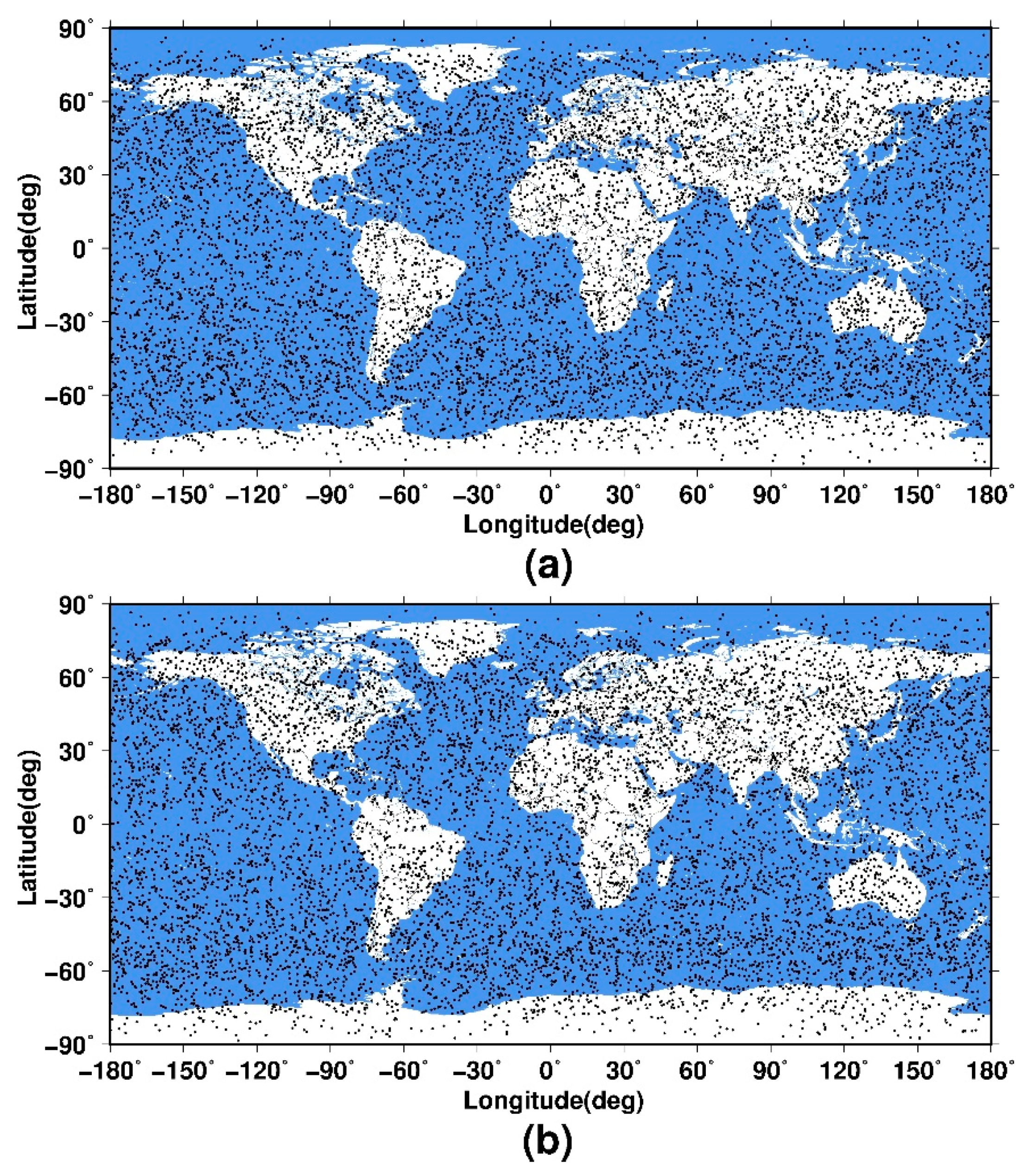
Figure 1 shows the distribution of the 24 h ROEs observed by COSMIC with five navigation satellite systems, including GPS, GLONASS, Galileo, BDS, and QZSS simulated based on their nominal constellation configurations. It should be mentioned that although COSMIC can only process the signals from GPS in practice, the number of ROEs can be expected to increase almost fourfold and better spatial and temporal distributions of ROEs will be acquired if the RO payload of COSMIC could track the signals from all the five navigation satellite systems. For the simulation of ROEs shown in Figure 1a, the real COSMIC orbits are applied. While for the simulation of ROEs shown in Figure 1b, the COSMIC orbits are simulated based on the initial satellite positions of the real orbits, using the Simplified General Perturbations Satellite Orbit Model 4 (SGP4) orbit propagator [45]. The number of the 24 h ROEs obtained based on the real and the simulated orbits is 10,317 and 10,340, respectively, with the relative difference of only 0.2%. It can be seen from Figure 1 that the distributions of the simulated 24 h ROEs in the two subfigures are very similar. Furthermore, the fitness value is 0.51968 and 0.51080 when the real and the simulated COSMIC orbits are used, respectively and the two values are very close to each other. These comparisons verify the effectiveness of the orbit simulation in this study.
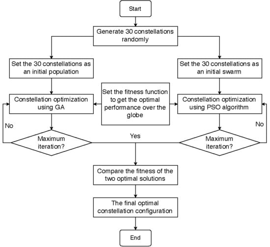
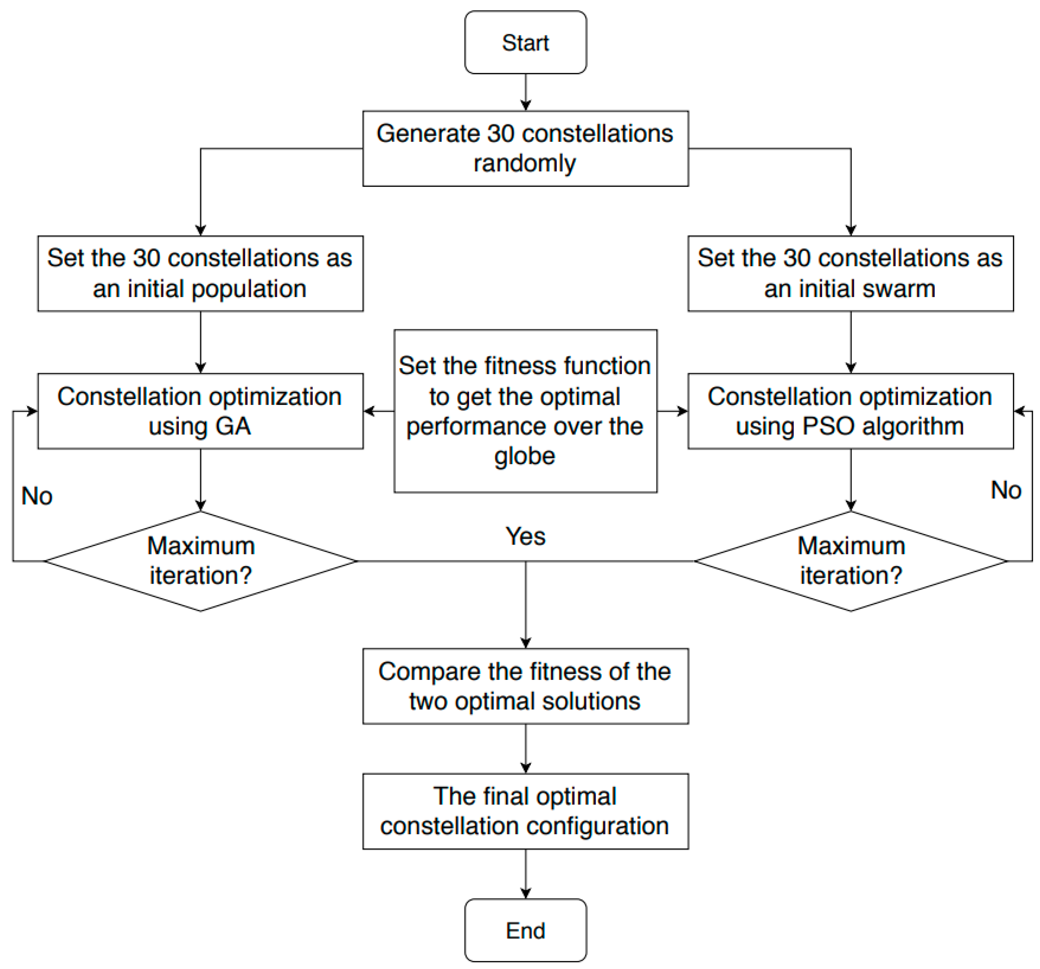
In the simulations conducted in this study, for a certain type of LEO constellation, it is assumed that the number of LEO satellites varies from 6 to 12. For a certain number of satellites and a certain constellation pattern, the flow chart to reach the optimal constellation configuration is presented in Figure 2. From this figure, it can be seen that the optimal constellation configuration which corresponds to the maximum value of the fitness function shown by Equation (6) is found with a GA and PSO, respectively, and the final optimal constellation configuration is the one with the highest fitness value resulted from the two optimal algorithms. It must be noted that, to ensure the fairness of the comparison between the two algorithms, the same termination condition (maximum iteration of 100 times), is set for both of the two evolutionary algorithms.
2.5. The Criteria to Evaluate the Performance of the ROE Distributions
Providing ROEs with a temporally and spatially uniform distribution is the critical issue for the design of LEO constellations in a GNSS RO mission. The performance of the temporal and spatial distribution of the ROEs is evaluated by the fitness function. Since the fitness function evaluates the optimality of the distribution of ROEs based on the spatial-temporal grids, it is not able to provide any insight into the point-to-point uniformity of ROEs in each grid and over the globe. Therefore, the uniformity in the spatial and temporal distribution of ROEs observed by the optimal LEO constellations are further assessed with the coefficient of variation (COV), which is defined to represent the uniformity degree of the point distribution [46] and is expressed as follows [47]:
where denotes the total number of ROEs, denotes the th ROE, is the minimal distance between the th ROE and its nearest neighbor and is the mean of all the values of . The smaller the COV, the smaller the variation of the minimal distance to its nearest neighbor, and the more uniform distribution of the points. A low value of COV corresponds to an ROE distribution close to a regular grid, so an optimized GNSS RO mission should be characterized by a low value of COV.
3. Results
3.1. Comparison of Evolutionary Algorithms
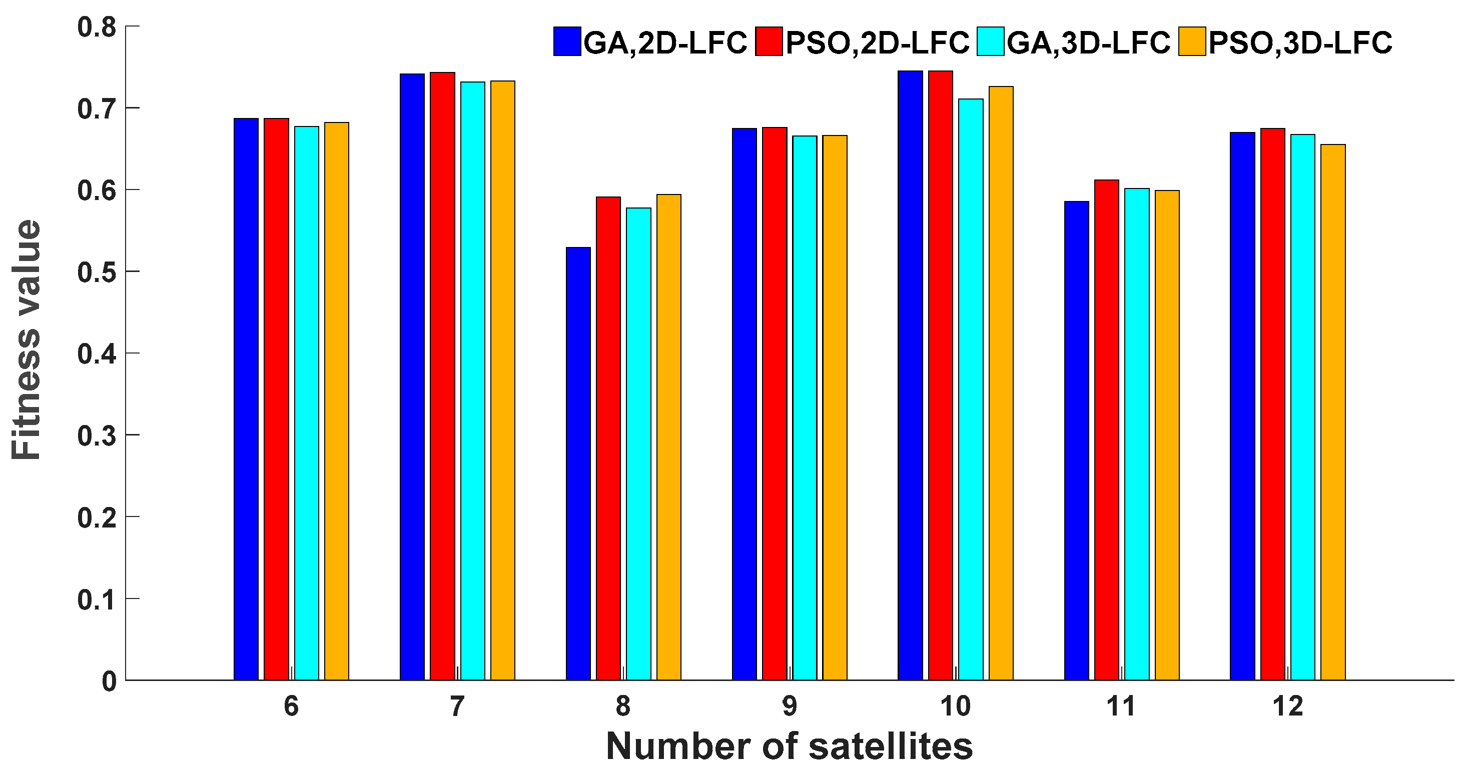
The optimal configurations for 2D-LFC or 3D-LFC composed of satellites are obtained separately based on the two different evolutionary algorithms, and the corresponding fitness values are compared in Figure 3. The higher the fitness value, the better the GNSS RO performance of the LEO constellation. As mentioned in Section 2.4, the same fitness function and number of iterations are applied in the two algorithms, which ensures the fairness of the comparison between them. In Figure 3, the comparison between the blue columns and the red columns shows that for the 2D-LFC pattern, the PSO algorithm always performs better than the GA over a varying number of LEO satellites between 6 and 12. The comparison between the green columns and the yellow columns shows that for the 3D-LFC pattern, a PSO algorithm also generally performs better than a GA except when and . So, for the LEO constellations composed of satellites, the final optimal 2D-LFCs and 3D-LFCs are generally (although not necessarily) the solutions of a PSO algorithm.
3.2. The Optimal Constellations
It is shown in Figure 3 that the constellation with the best result depends on the optimization algorithm. Regarding the dependency on the algorithm, the two methods are considered and the better solution achieved by either of them, which corresponds to the highest fitness value, is selected. Table 4 and Table 5 presents the parameters defining the final optimal 2D-LFCs and 3D-LFCs composed of satellites, respectively. It is shown that, regardless of the constellation pattern and number of satellites, the inclination angles of the optimized constellations are generally high, which is important for obtaining a uniform temporal and spatial distribution over the globe. It is also shown that the altitudes of the satellites in both 2D-LFCs and 3D-LFCs are generally lower than 650 km. Moreover, the fitness values of the final optimized constellations are generally higher than 0.6, which means that the numbers of spatio-temporal grids with ROEs more than the expected, are generally larger than 3000.
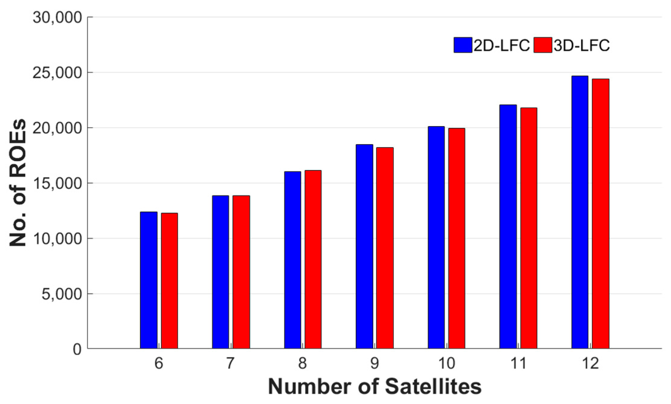
Figure 4 presents the numbers of the 24 h GNSS ROEs observed by the final optimal LEO constellations with 2D-LFC and 3D-LFC patterns composed of satellites. It can be seen that for a certain number of LEO satellites, the numbers of ROEs observed by the optimal configurations of 2D-LFC and 3D-LFC are very close to each other, while the number of the ROEs observed by the optimized 2D-LFC is slightly larger than those observed by the optimized 3D-LFC.
Figure 4 also shows that the more LEO satellites, the more GNSS ROEs will be observed. With 12 LEO satellites, the number of 24 h GNSS ROEs observed by the optimized LEO constellations increases up to almost 25,000.
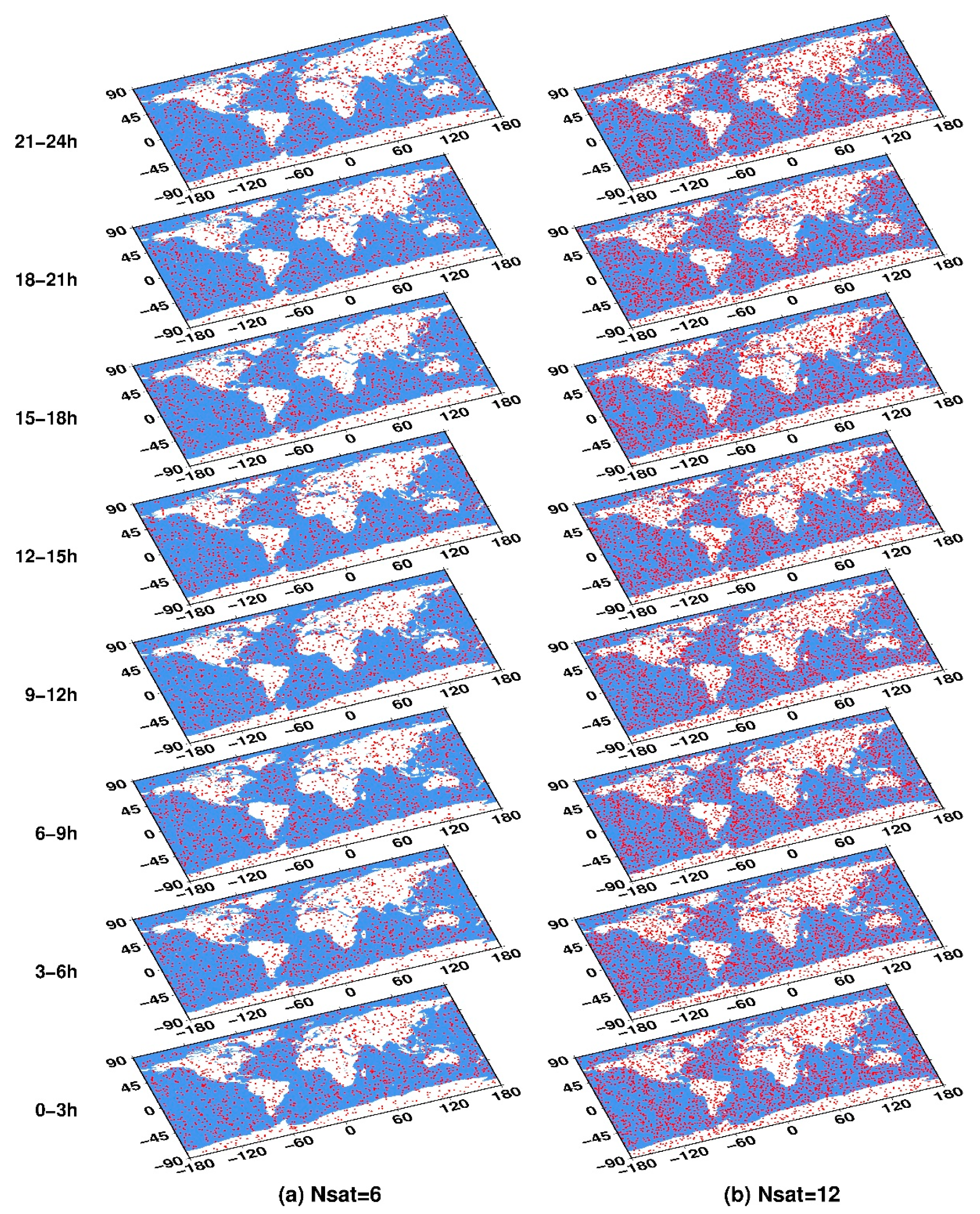
The spatial and temporal distributions of the ROEs observed by all the final optimized LEO constellations can be presented visually. Here, as representatives, the spatial distributions of the ROEs in 3 h intervals for one day, observed by the final optimized 2D-LFCs composed of 6 and 12 LEO satellites, are shown in Figure 5. It can be seen that as the number of satellites increases, the number of ROEs observed in each three hours increases accordingly. Independently from the number of satellites, the distributions of the ROEs observed by the optimized configurations within each 3 h are homogeneous over the globe.
3.3. Performance Evaluation of the Optimal Constellations
As mentioned in Section 2.5, a uniform point-to-point distribution should be characterized by a low COV value. Hence, after the optimal constellations are obtained based on the evolutionary algorithms, their performances for GNSS RO observation over the globe are further evaluated using the COV. For each optimal constellation, the COV value corresponding to the ROE distribution within each 3 h is calculated. Therefore, there are 8 COV values for one day. The mean and standard deviation of the 8 COV values are also reported in Table 6. For a certain number of satellites, the optimal configurations for the two LEO constellation patterns are compared according to the means and standard deviations listed in this table. The smaller the mean and standard deviation, the better the performance of the LEO constellation.
According to Table 6, as the number of satellites varies between 6 and 12, all the optimized 2D-LFCs and 3D-LFCs provide mean COV values for 3 h-distributions of ROEs lower than 0.6 and most of the standard deviations of the COV values are lower than 0.02. This indicates that both the optimal 2D-LFC and 3D-LFC configurations are of proper point-to-point ROE distributions in each 3 h, and the temporal variation of the observation uniformity is generally small.
Table 6 also shows that, among the seven choices for the number of LEO satellites , the COV mean values of the optimal 2D-LFCs are lower than those of the optimal 3D-LFCs with . For the other two constellations, the COV mean values provided by 3D-LFCs are slightly higher. This indicates that the optimized 2D-LFCs generally result in slightly more uniform point-to-point distributions of 3 h-ROEs compared to the optimized 3D-LFCs. As the number of LEO satellites varies between 6 and 12, the standard deviations of the COV values for the optimal 2D-LFCs are mostly lower than the corresponding optimal 3D-LFCs, which shows that the temporal variations of the ROEs distribution from 2D-LFCs are mostly smaller than those from the optimized 3D-LFCs.
3.4. Comparison with the COSMIC Constellation
The performance of the optimal 2D-LFC and 3D-LFC configurations composed of six satellites are further compared with the existing RO mission, COSMIC. Table 7 presents the detailed information about the number of 24 h simulated ROEs, the corresponding fitness values, and the mean 3 h-COVs of the two optimized LEO constellations as well as COSMIC. It can be seen that both of the two optimized configurations can observe more ROEs than COSMIC, and the number of ROEs observed by the optimal 2D-LFC is the largest among the three constellations. The fitness values of the two optimal constellations are both larger than that of COSMIC, while the mean 3 h-COV values of the two optimal constellations are both lower. This indicates that the spatial and temporal distributions of the ROEs observed by the two optimal configurations are more uniform than the ROEs observed by COSMIC. In particular, it should be noted that the performance of the optimized 2D-LFC is the best among the three LEO constellations.
4. Discussion
As introduced in Section 2.3, the fitness function used in the evolutionary algorithms is based on the concept of a spatio-temporal point pattern. In Equation (6), represents the total number of spatio-temporal grids over the globe for one day, hence, the degree of the optimization both in the spatial and temporal ROEs distribution is taken into consideration by this fitness function. Searching for the optimal 12 satellite walker constellation for GNSS RO observation with a GA algorithm, Juang et al. [24] used a fitness function similar to Equation (6), while the spatio-temporal grids of were used and there was no evaluation of the temporal distribution of ROEs during one day. Furthermore, here in Equation (6), , the expected mean number of ROEs of each spatio-temporal grid, was calculated based on the total number of simulated 24 h ROEs over the globe and the number of spatio-temporal grids, while this parameter was just simplified to be equal to 4 in the study by Juang et al. [24].
Both Juang et al. [24] and Asgarimehr et al. [26] used a GA to search for the optimal LEO constellation configuration for GNSS RO performance over the target region. Considering that the optimized constellation configuration sought depends on the optimization algorithm used, it stands to reason to use more than one evolutionary algorithm in the optimization process only if the comparison between the algorithms is fair [27]. Hence, both a GA and PSO were applied in our study. To ensure the fairness of the comparison between the two algorithms, the evolutionary processes were iterated the same number of times (100 generations) in each algorithm. It was found that regardless of the constellation pattern, the PSO algorithm generally (although not necessary) performed better than a GA, which means that the spatial and temporal distributions of ROEs, observed by the optimal constellations obtained by the PSO algorithm, are generally better compared to those derived by GA.
As to the comparison between the two constellation patterns, Asgarimehr et al. [26] found that for a LEO constellation composed of six satellites, the daily number of GPS ROEs, which occur over the Asia and Pacific region observed by the optimized 2D-LFC, is larger than those observed by the optimized 3D-LFC. Our study further confirms that for a LEO constellation composed of satellites, the optimized 2D-LFCs generally could observe more GNSS ROEs over the globe compared with the optimized 3D-LFCs. In Reference [26], the altitudes of the circular orbits in the optimized 2D-LFC are lower than those of the elliptical orbits in the optimized 3D-LFC. In our study, the comparison between Table 4 and Table 5 also revealed that, for a LEO constellation composed of satellites, with the whole globe as the target region of GNSS RO observation, all the circular orbits in the optimized 2D-LFC were lower in height than the elliptical orbits of the optimized 3D-LFC. Juang et al. [24] found that high inclinations of LEO satellites are beneficial for a sufficient global coverage of the ROEs. All the optimal 2D-LFCs and 3D-LFCs were of high inclinations in our study, which are shown by Table 4 and Table 5.
The comparisons of the COV mean values and its standard deviation between the two different constellation patterns show that, as the number of LEO satellites varies between 6 and 12, the GNSS ROEs observed by the optimized 2D-LFCs were generally more homogeneous in space and time compared to the optimized 3D-LFCs. The comparison of the optimized 6 satellite 2D-LFC and 3D-LFC with COSMIC further approved the superiority of the optimized 2D-LFC performance.
5. Conclusions
Exploiting the navigation signals from the GPS, GLONASS, BDS, Galileo, and QZSS, the present work focused on the search for a 2D-LFC and 3D-LFC composed of 6–12 satellites, which could provide optimal spatial and temporal distributions of GNSS ROEs over the globe. Two evolutionary algorithms were applied with a fitness function based on the concept of spatio-temporal point pattern. The better solution obtained by either of them, which corresponded to the highest fitness value, was selected. The space-filling performance of the final optimal LEO constellations were further evaluated using COVs of the distribution of ROEs.
The results showed that with the use of multi-GNSS signals, the optimized constellation configurations provided a sufficient number of ROEs with proper temporal and spatial distributions. For a certain number of LEO satellites, a PSO algorithm generally performed better than a GA. The optimal 2D-LFC generally resulted in higher fitness values compared to the optimal 3D-LFC. In other words, 2D-LFC observed more uniform ROE distributions in time and space. This is further confirmed by the comparisons of the mean and standard deviations values of the 3 h-COV for one day.
In our future work, the 2D necklace flower constellation, which accelerates the generation of constellations in the optimization process with more control in the design, will be taken into consideration and the proposed fitness function for the evolutionary algorithms will be further improved in the design of LEO constellations for GNSS RO mission.
Author Contributions
X.X., Y.H. and J.L. conceptualized the initial idea and experiment design; Y.H. analyzed the data; X.X., Y.H. and J.L. wrote the main manuscript text; J.W. and M.A. reviewed the paper and provided valuable insights.
Funding
This research was funded by the National Natural Science Foundation of China (Grant No. 41774033 and 41774032), the National Key Research and Development Program of China (Grant No. 2018YFC1503502), and the National Basic Research Program of China (973 Program) (Grant No. 2013CB733302).
Conflicts of Interest
The authors declare no conflict of interests.
References
- Arnas, D.; Casanova, D.; Tresaco, E. 2D necklace flower constellations. Acta Astronaut. 2018, 142, 18–28. [Google Scholar] [CrossRef]
- Kliore, A.; Cain, D.L.; Levy, G.S.; Eshleman, V.R.; Fjeldbo, G.; Drake, F.D. Occultation experiment: Results of the first direct measurement of Mars’s atmosphere and ionosphere. Science 1965, 149, 1243–1248. [Google Scholar] [CrossRef] [PubMed]
- Bevis, M.; Businger, S.; Chiswell, S.; Herring, T.A.; Anthes, R.A.; Rocken, C.; Ware, R.H. GPS Meteorology: Mapping zenith wet delays onto Precipitable water. J. Appl. Meteorol. 1994, 33, 379–386. [Google Scholar] [CrossRef]
- Ware, R.; Exner, M.; Feng, D.; Gorbunov, M.; Hardy, K.; Herman, B.; Kuo, Y.; Meehan, T.; Melbourne, W.; Rocken, C.; et al. GPS sounding of the atmosphere from low Earth orbit: Preliminary results. Bull. Am. Meteorol. Soc. 1996, 77, 19–40. [Google Scholar] [CrossRef]
- Wickert, J.; Reigber, C.; Beyerle, G.; König, R.; Marquardt, C.; Schmidt, T.; Grunwaldt, L.; Galas, R.; Meehan, T.K.; Melbourne, W.G.; et al. Atmosphere sounding by GPS radio occultation: First results from CHAMP. Geophys. Res. Lett. 2001, 28, 3263–3266. [Google Scholar] [CrossRef] [Green Version]
- Anthes, R.A. Exploring Earth’s atmosphere with radio occultation: Contributions to weather, climate and space weather. Atmos. Meas. Tech. 2011, 4, 1077–1103. [Google Scholar] [CrossRef]
- Bartalis, Z.; Wagner, W.; Naeimi, V.; Hasenauer, S.; Scipal, K.; Bonekamp, H.; Figa, J.; Anderson, C. Initial soil moisture retrievals from the METOP-A Advanced Scatterometer (ASCAT). Geophys. Res. Lett. 2007, 34, 20. [Google Scholar] [CrossRef]
- Klaes, K.D.; Montagner, F.; Larigauderie, C. Metop-B, the second satellite of the EUMETSAT polar system, in orbit. Earth Observing Systems XVIII. Int. Soc. Opt. Photonics 2013, 8866, 886613. [Google Scholar]
- Bi, Y.; Yang, Z.; Zhang, P.; Sun, Y.; Bai, W.; Du, Q.; Yang, G.; Chen, J.; Liao, M. An introduction to China FY3 radio occultation mission and its measurement simulation. Adv. Space Res. 2012, 49, 1191–1197. [Google Scholar] [CrossRef]
- Schreiner, W.; Rocken, C.; Sokolovskiy, S.; Syndergaard, S.; Hunt, D. Estimates of the precision of GPS radio occultations from the COSMIC/FORMOSAT-3 mission. Geophys. Res. Lett. 2007, 34. [Google Scholar] [CrossRef] [Green Version]
- Wickert, J.; Michalak, G.; Schmidt, T.; Beyerle, G.; Cheng, C.Z.; Healy, S.B.; Heise, S.; Huang, C.Y.; Jakowski, N.; Köhler, W.; et al. GPS radio occultation: Results from CHAMP, GRACE and FORMOSAT-3/COSMIC. Terr. Atmos. Ocean. Sci. 2009, 20, 35–50. [Google Scholar] [CrossRef]
- Cucurull, L. Improvement in the use of an operational constellation of GPS radio occultation receivers in weather forecasting. Weather Forecast. 2010, 25, 749–767. [Google Scholar] [CrossRef]
- Steiner, A.K.; Lackner, B.C.; Ladstädter, F.; Scherllin-Pirscher, B.; Foelsche, U.; Kirchengast, G. GPS radio occultation for climate monitoring and change detection. Radio Sci. 2011, 46, 1–17. [Google Scholar] [CrossRef]
- Lei, J.; Syndergaard, S.; Burns, A.G.; Solomon, S.C.; Wang, W.; Zeng, Z.; Roble, R.G.; Wu, Q.; Kuo, Y.H.; Holt, J.M.; et al. Comparison of COSMIC ionospheric measurements with ground-based observations and model predictions: Preliminary results. J. Geophys. Res. Space Phys. 2007, 112. [Google Scholar] [CrossRef] [Green Version]
- Hsu, C.T.; Matsuo, T.; Yue, X.; Fang, T.W.; Fuller-Rowell, T.; Ide, K.; Liu, J.Y. Assessment of the Impact of FORMOSAT-7/COSMIC-2 GNSS RO Observations on Midlatitude and Low-Latitude Ionosphere Specification: Observing System Simulation Experiments Using Ensemble Square Root Filter. J. Geophys. Res. Space Phys. 2018, 123, 2296–2314. [Google Scholar] [CrossRef]
- Jakowski, N.; Wilken, V.; Schlueter, S.; Stankov, S.M.; Heise, S. Ionospheric space weather effects monitored by simultaneous ground and space based GNSS signals. J. Atmos. Sol. Terr. Phys. 2005, 67, 1074–1084. [Google Scholar] [CrossRef]
- Tseng, T.P.; Chen, S.Y.; Chen, K.L.; Huang, C.Y.; Yeh, W.H. Determination of near real-time GNSS satellite clocks for the FORMOSAT-7/COSMIC-2 satellite mission. GPS Solut. 2018, 22, 47. [Google Scholar] [CrossRef]
- Bai, W.H.; Sun, Y.Q.; Du, Q.; Yang, G.L.; Yang, Z.D.; Zhang, P.; Bi, Y.M.; Wang, X.Y.; Cheng, C.; Han, Y. An introduction to the fy3 gnos instrument and mountain-top tests. Atmos. Meas. Tech. 2014, 7, 1817–1823. [Google Scholar] [CrossRef]
- Liao, M.; Zhang, P.; Yang, G.L.; Bi, Y.M.; Liu, Y.; Bai, W.H.; Meng, X.G.; Du, Q.F.; Sun, Y.Q. Preliminary validation of the refractivity from the new radio occultation sounder GNOS/FY-3C. Atmos. Meas. Tech. 2016, 9, 781–792. [Google Scholar] [CrossRef] [Green Version]
- Sun, Y.; Liu, C.; Du, Q.; Wang, X.; Bai, W.; Kirchengast, G.; Xia, J.; Meng, X.; Wang, D.; Cai, Y.; et al. Global Navigation Satellite System Occultation Sounder II (GNOS II). In Proceedings of the 2017 IEEE International Geoscience and Remote Sensing Symposium (IGARSS), Fort Worth, TX, USA, 23–28 July 2017; pp. 1189–1192. [Google Scholar]
- Mousa, A.; Aoyama, Y.; Tsuda, T. A simulation analysis to optimize orbits for a tropical GPS radio occultation mission. Earth Planets Space 2006, 58, 919–925. [Google Scholar] [CrossRef] [Green Version]
- Xu, X.; Li, Z.; Luo, J. Simulation of the impacts of single LEO satellite orbit parameters on the distribution and number of occultation events. Geo-Spat. Inf. Sci. 2006, 9, 13–17. [Google Scholar] [CrossRef] [Green Version]
- Chern, R.J.S.; Huang, C.M. Effect of orbit inclination on the performance of FORMOSAT-3/-7 type constellations. Acta Astronaut. 2013, 82, 47–53. [Google Scholar] [CrossRef]
- Juang, J.C.; Tsai, Y.F.; Chu, C.H. On constellation design of multi-GNSS radio occultation mission. Acta Astronaut. 2013, 82, 88–94. [Google Scholar] [CrossRef]
- Lee, S.; Mortari, D. 2-D Lattice Flower Constellations for Radio Occultation Missions. Front. Aerosp. Eng. 2013, 2, 79–90. [Google Scholar]
- Asgarimehr, M.; Hossainali, M.M. GPS radio occultation constellation design with the optimal performance in Asia Pacific region. J. Geod. 2015, 89, 519–536. [Google Scholar] [CrossRef]
- Casanova, D.; Avendaño, M.; Mortari, D. Seeking GDOP-optimal Flower Constellations for global coverage problems through evolutionary algorithms. Aerosp. Sci. Technol. 2014, 39, 331–337. [Google Scholar] [CrossRef]
- Zhu, X.; Gao, Y. Comparison of Intelligent Algorithms to Design Satellite Constellations for Enhanced Coverage Capability. In Proceedings of the 2017 10th International Symposium on Computational Intelligence and Design, Hangzhou, China, 9–10 December 2017; pp. 223–226. [Google Scholar] [CrossRef]
- Fossa, C.E.; Raines, R.A.; Gunsch, G.H.; Temple, M.A. An overview of the IRIDIUM (R) low Earth orbit (LEO) satellite system. In Proceedings of the IEEE 1998 National Aerospace and Electronics Conference, Dayton, OH, USA, 17 July 1998; pp. 152–159. [Google Scholar]
- Dietrich, F.J.; Metzen, P.; Monte, P. The Globalstar cellular satellite system. IEEE Trans. Antennas Propag. 1998, 46, 935–942. [Google Scholar] [CrossRef]
- Avendaño, M.E.; Davis, J.J.; Mortari, D. The 2-D lattice theory of flower constellations. Celest. Mech. Dyn. Astron. 2013, 116, 325–337. [Google Scholar] [CrossRef]
- Davis, J.J.; Avendaño, M.E.; Mortari, D. The 3-D lattice theory of flower constellations. Celest. Mech. Dyn. Astron. 2013, 116, 339–356. [Google Scholar] [CrossRef]
- Speckman, L.; Lang, T.; Boyce, W. An analysis of the line of sight vector between two satellites in common altitude circular orbits. In Proceedings of the Astrodynamics Conference, Portland, OR, USA, 20–22 August 1990; p. 2988. [Google Scholar] [CrossRef]
- Asvial, M.; Tafazolli, R.; Evans, B.G. Satellite constellation design and radio resource management using genetic algorithm. IEE Proc. Commun. 2004, 151, 204–209. [Google Scholar] [CrossRef]
- Fonseca, C.M.; Fleming, P.J. Genetic Algorithms for Multiobjective Optimization: Formulation Discussion and Generalization. Icga 1993, 93, 416–423. [Google Scholar]
- Goldber, D.E.; Holland, J.H. Genetic algorithms and machine learning. Mach. Learn. 1988, 3, 95–99. [Google Scholar] [CrossRef]
- Eberhart, R.; Shi, Y. Particle swarm optimization: Developments, applications and resources. In Proceedings of the 2001 Congress on Evolutionary Computation, Seoul, Korea, 27–30 May 2001; Volume 1, pp. 81–86. [Google Scholar] [CrossRef]
- Cox, D.R.; Isham, V. Point Processes; Chapman and Hall: London, UK, 1980; pp. 159–166. [Google Scholar]
- Gabriel, E.; Rowlingson, B.; Diggle, P. stpp: An R package for plotting, simulating and analyzing Spatio-Temporal Point Patterns. J. Stat. Softw. 2013, 53, 1–29. [Google Scholar] [CrossRef]
- CSNO. BeiDou Navigation Satellite System Signal in Space Interface Control Document; Version 1.0; China Satellite Navigation Office: Beijing, China, 2018.
- DOD SPS, Department of Defense USA. Global Positioning System Standard Positioning Service Performance Standard, 4th ed. 2008. Available online: http://www.gps.gov/technical/ps/2008-SPS-performancestandard (accessed on 6 January 2012).
- GLONASS Interface Control Document ICD. Navigational Radiosignal in Bands L1, L2, 5.1th ed.; Russian Institute of Space Device Engineering: Moscow, Russia, 2008. [Google Scholar]
- OS-SIS-ICD. European GNSS (Galileo) Open Service Signal in Space Interface Control Document, SISICD-2006; European Space Agency: Paris, France, 2010. [Google Scholar]
- Jaxa. Quasi-Zenith Satellite System Navigation Service Interface Specification for QZSS (IS-QZSS) version 1.4; Japan Aerospace Exploration Agency: Tokyo, Japan, 2012. [Google Scholar]
- Hoots, F.R.; Roehrich, R.L. Models for Propagation of NORAD Element Sets. Aerospace Defense Command Peterson Afb Co Office of Astrodynamics. 1980. Available online: http://large.stanford.edu/courses/2017/ph241/summerville2/docs/a093554.pdf (accessed on 28 March 2017).
- Romero, V.; Burkardt, J.; Gunzburger, M.; Peterson, J. Initial evaluation of pure and ‘‘latinized’’ centroidal Voronoi tessellation for non-uniform statistical sampling. In Proceedings of the Sensitivity Analysis of Model Output Conference, Santa Fe, NM, USA, 8–11 March 2004. [Google Scholar]
- Gunzburger, M.; Burkardt, J. Uniformity measures for point sample in hypercubes. Rapp. Tech. Fla. State Univ. 2004, 25, 73. [Google Scholar]
Figure 1.
The simulated 24 h Global Navigation Satellite System (GNSS) radio occultation events (ROEs), observed by COSMIC using the real orbits (a) and the simulated orbits (b).
Figure 1.
The simulated 24 h Global Navigation Satellite System (GNSS) radio occultation events (ROEs), observed by COSMIC using the real orbits (a) and the simulated orbits (b).

Figure 2.
The optimization algorithm flowchart of the LEO constellation with certain number of satellites and certain constellation pattern.
Figure 2.
The optimization algorithm flowchart of the LEO constellation with certain number of satellites and certain constellation pattern.

Figure 3.
Fitness values of the optimal configurations for 2D-lattice flower constellation (2D-LFC) and 3D-LFC composed of 6-12 satellites based on Genetic Algorithm (GA) and Particle Swarm Optimization (PSO) algorithms.
Figure 3.
Fitness values of the optimal configurations for 2D-lattice flower constellation (2D-LFC) and 3D-LFC composed of 6-12 satellites based on Genetic Algorithm (GA) and Particle Swarm Optimization (PSO) algorithms.

Figure 4.
The numbers of ROEs observed in one day by the final optimal LEO constellations with 2D-LFC and 3D-LFC patterns composed of 6–12 satellites.
Figure 4.
The numbers of ROEs observed in one day by the final optimal LEO constellations with 2D-LFC and 3D-LFC patterns composed of 6–12 satellites.

Figure 5.
The distribution of ROEs observed within each three hours of one day by the final optimal LEO constellations with 2D-LFC pattern composed of 6 (a) and 12 satellites (b).
Figure 5.
The distribution of ROEs observed within each three hours of one day by the final optimal LEO constellations with 2D-LFC pattern composed of 6 (a) and 12 satellites (b).


Table 1.
The variation range of the parameters defining 2D-lattice flower constellation (2D-LFC) composed of satellites.
Table 1.
The variation range of the parameters defining 2D-lattice flower constellation (2D-LFC) composed of satellites.
| Parameter | Variation Range |
|---|---|
| i | [1°,100°] |
| orbit altitude | |
* denotes all the divisors of .
Table 2.
The variation range of the parameters defining 3D-LFC composed of satellites.
| Parameter | Variation Range |
|---|---|
| i | [1°,100°] |
| e | [0.01,0.05] |
| orbit altitude | |
* and denotes the divisors of which satisfy that is also the divisor of .
Table 3.
The configurations for the five nominal Global Navigation Satellite System (GNSS) constellations.
Table 3.
The configurations for the five nominal Global Navigation Satellite System (GNSS) constellations.
| System | GPS | GLONASS | Galileo | BDS | QZSS | |||
|---|---|---|---|---|---|---|---|---|
| Orbit | MEO | MEO | MEO | MEO | IGSO | GEO | QZO | GEO |
| Number of satellites | 24 | 24 | 24 | 24 | 3 | 3 | 3 | 1 |
| Constellation pattern | 6 planes | Walker (24/3/1) * | Walker (24/3/1) | Walker (24/3/1) | / | / | / | / |
| Inclination [deg] | 56 | 64.8 | 56 | 55 | 55 | 0 | 43 | 0 |
| Altitude (km) | 20,180 | 19,100 | 23,220 | 21,528 | 35,786 | 35,786 | 35,786 | 35,786 |
* t/p/f where t denotes the total number of satellites, p is the number of equally spaced planes, and f is the relative spacing between satellites in adjacent planes.
Table 4.
The parameters of the optimal 2D-LFC configurations.
| Nsat | Orbit Altitude (km) | i(°) | No | Nso | Nc | Fitness Value |
|---|---|---|---|---|---|---|
| 6 | 415.471 | 90.398 | 3 | 2 | 1 | 0.68692 |
| 7 | 477.085 | 87.532 | 7 | 1 | 4 | 0.74325 |
| 8 | 500.825 | 97.762 | 8 | 1 | 3 | 0.59105 |
| 9 | 491.636 | 90.274 | 3 | 3 | 1 | 0.67593 |
| 10 | 430.506 | 90.462 | 5 | 2 | 2 | 0.74518 |
| 11 | 483.447 | 90.488 | 11 | 1 | 1 | 0.61188 |
| 12 | 467.620 | 90.697 | 3 | 4 | 1 | 0.67438 |
Table 5.
The parameters of the optimal 3D-LFC configurations.
| Nsat | Orbit Altitude (km) | i(°) | e | No | Nw | Nso | Nc1 | Nc2 | Nc3 | Fitness Value |
|---|---|---|---|---|---|---|---|---|---|---|
| 6 | 520.038 | 89.617 | 0.01 | 3 | 1 | 2 | 3 | 1 | 2 | 0.68191 |
| 7 | 505.997 | 88.544 | 0.01 | 7 | 1 | 1 | 2 | 1 | 2 | 0.73264 |
| 8 | 529.264 | 99.078 | 0.01 | 8 | 1 | 1 | 3 | 1 | 2 | 0.59394 |
| 9 | 633.961 | 89.317 | 0.02 | 3 | 1 | 3 | 1 | 1 | 2 | 0.66609 |
| 10 | 572.877 | 92.260 | 0.01 | 5 | 2 | 1 | 1 | 2 | 2 | 0.72608 |
| 11 | 532.137 | 89.130 | 0.02 | 11 | 1 | 1 | 1 | 1 | 1 | 0.60108 |
| 12 | 537.006 | 89.130 | 0.01 | 3 | 1 | 4 | 1 | 1 | 1 | 0.66744 |
Table 6.
The mean and the standard deviations of the COV values for 3 h-distributions of radio occultation events (ROEs) during one day for the optimal 2D-LFCs and 3D-LFCs composed of 6–12 satellites.
Table 6.
The mean and the standard deviations of the COV values for 3 h-distributions of radio occultation events (ROEs) during one day for the optimal 2D-LFCs and 3D-LFCs composed of 6–12 satellites.
| No. of Satellites | 2D-LFC | 3D-LFC | ||
|---|---|---|---|---|
| Mean | Std | Mean | Std | |
| 6 | 0.54143 | 0.015 | 0.56178 | 0.032 |
| 7 | 0.53720 | 0.012 | 0.54028 | 0.017 |
| 8 | 0.54756 | 0.012 | 0.55244 | 0.010 |
| 9 | 0.54228 | 0.014 | 0.53344 | 0.014 |
| 10 | 0.53065 | 0.011 | 0.54203 | 0.019 |
| 11 | 0.54780 | 0.012 | 0.53644 | 0.018 |
| 12 | 0.54112 | 0.014 | 0.54328 | 0.015 |
Table 7.
The comparison of the performances of the optimized six-satellite 2D-LFC, 3D-LFC with COSMIC.
Table 7.
The comparison of the performances of the optimized six-satellite 2D-LFC, 3D-LFC with COSMIC.
| COSMIC | 2D-LFC | 3D-LFC | |
|---|---|---|---|
| No. of 24 h ROEs | 10,340 | 12,386 | 12,250 |
| Fitness value | 0.51080 | 0.68692 | 0.68191 |
| Mean 3 h- COV | 0.62081 | 0.54143 | 0.56178 |
© 2019 by the authors. Licensee MDPI, Basel, Switzerland. This article is an open access article distributed under the terms and conditions of the Creative Commons Attribution (CC BY) license (http://creativecommons.org/licenses/by/4.0/).
Share and Cite
MDPI and ACS Style
Xu, X.; Han, Y.; Luo, J.; Wickert, J.; Asgarimehr, M. Seeking Optimal GNSS Radio Occultation Constellations Using Evolutionary Algorithms. Remote Sens. 2019, 11, 571. https://0-doi-org.brum.beds.ac.uk/10.3390/rs11050571
AMA Style
Xu X, Han Y, Luo J, Wickert J, Asgarimehr M. Seeking Optimal GNSS Radio Occultation Constellations Using Evolutionary Algorithms. Remote Sensing. 2019; 11(5):571. https://0-doi-org.brum.beds.ac.uk/10.3390/rs11050571
Chicago/Turabian StyleXu, Xiaohua, Yi Han, Jia Luo, Jens Wickert, and Milad Asgarimehr. 2019. "Seeking Optimal GNSS Radio Occultation Constellations Using Evolutionary Algorithms" Remote Sensing 11, no. 5: 571. https://0-doi-org.brum.beds.ac.uk/10.3390/rs11050571
Note that from the first issue of 2016, this journal uses article numbers instead of page numbers. See further details here.