Identification of the Best Hyperspectral Indices in Estimating Plant Species Richness in Sandy Grasslands

Abstract

Numerous spectral indices have been developed to assess plant diversity. However, since they are developed in different areas and vegetation type, it is difficult to make a comprehensive comparison among these indices. The primary objective of this study was to explore the optimum spectral indices that can predict plant species richness across different communities in sandy grassland. We use 7339 spectral indices (7217 we developed and 122 that were extracted from literature) to predict plant richness using a two-year dataset of plant species and spectra information at 270 plots. For this analysis, we employed cluster analysis, correlation analysis, and stepwise linear regression. The spectral variability within the 420–480 nm and 760–900 nm ranges, the first derivative value at the sensitive bands, and the normalized difference at narrow spectral ranges correlated well with plant species richness. Within the 7339 indices that were investigated, the first-order derivative values at 606 and 583 nm, the reflectance combinations on red bands: (R802 − R465)/(R802 + R681) and (R750 − R550)/(R750 + R550) showed a stable performance in both the independent calibration and validation datasets (R² > 0.27, p < 0.001, RMSE < 1.7). They can be regarded as the best spectral indices to estimate plant species richness in sandy grasslands. In addition to these spectral variation indices, the first derivative values or the normalized difference of the sensitive bands also reflect plant diversity. These results can help to improve the estimation of plant diversity using satellite-based airborne and hand-held hyperspectral sensors.

1. Introduction

Plant species diversity is a key element in the provision of ecosystem services [1,2]. Species richness refers to the total number of species in a sampling unit and it is a strong indicator of plant diversity [3]. In the electromagnetic spectrum, different plant species respond differently to light radiation [4,5]. Thus, the variations in the remotely sensed spectra can be used to assess plant species diversity. This forms a key basis in the Spectral Variations Hypothesis (SVH) [3,6,7,8]. This means that spectral entropy is potentially represents an efficient and relatively inexpensive means to provide biodiversity estimates when compared to high-cost, labor-intensive field surveys [9]. Theoretically, the greater the detail contained within a spectral range of a remotely sensed data-set, the more useful it will be extract reliable predictors of plant.

Numerous spectral indices have been developed to predict plant species diversity. The red (630–690 nm) and near infrared (NIR, 760–900 nm) wavebands, which are known to reflect vegetation structure, are always commonly selected to predict species diversity at a plot scale [10]. The normalized difference vegetation index (NDVI), calculated based on the red and infrared (IR) bands, and its variations of this index, are frequently used as indicators of plant species richness [10,11,12]. The enhanced vegetation index (EVI) [13], infrared index (IRI), middle infrared index (MIRI), atmosphere resistance vegetation index (ARVI), and soil-adjusted vegetation index (SAVI) have also been found to be closely related to plant species diversity [14,15]. The mean Euclidean distances between the spectral clusters derived from Principal Component Analysis (PCA) has also been used to predict plant species diversity [3,8]. First- and second-order derivative values of reflectance [16,17] and their standard deviations have been used in regression analysis again provided good predictors of plant diversity [18]. The first- and second- order in variations of the EVI have been found to be superior in assessing plant diversity when compared to the other commonly used parameters [19]. To date, these spectral indices have been generally calculated based on narrow wavebands, which were selected based on empirical vegetation indices or the biochemical absorption domain in the plant spectra. Most of the indices are also strongly site-dependent, and only accurate at the site where they were developed. Reasons for this strong site-dependence may be differences in (a) the resolution of the applied remote-sensing data, (b) the spatial dimensions of field plots [20], (c) the spectral resolution, and/or (d) the timing of field investigation [21]. To compare the different indices and identify the best ones is extremely important to broaden the use of remote sensing in assessing plant diversity throughout the world. Nevertheless, thus far no attempt has been made to compare the entire set of indices published to date and identify the best ones for estimating plant species richness.

Hyperspectral data can provide hundreds of bands with 1–10 nm resolution. Numerous spectral indices, both newly developed and previously published, can be established based on the hundreds of wavebands that are contained in this data. Owing to this advantage, hyperspectral data has been successfully used to estimate plant diversity of temperate forest [22], rainforest [23], tropical forest [24,25], savanna [3], heterogeneous forest [26], alpine grassland [27], grazed dry grassland [28], and sandy grassland [29]. Based on the very distinct variability in the absorption and reflectance properties of individual bands. The Hunshandak Sandland sandy grassland, which is located in the Euro-Asian biome, represents one of the most species-rich Asia grassland ecosystems. To date, assessments of this area’s plant species diversity using remote sensing are lacking. In this study, 270 circular plots with a 0.8m diameter were surveyed, and 7339 spectral indices (122 published and 7217 newly developed) were extracted for each of these plots, to address the persisting knowledge gaps by focusing on the following three research questions:

• Within the thousands of hyperspectral indices, which ones perform best in estimating species richness?
• Does the hyperspectral data conform to predictions based on the Spectral Variations Hypothesis?
• How well do the investigated hyperspectral spectral indices perform as a proxy for plant species richness under different vegetation cover and structural complexity?

To answer these questions, we surveyed the vegetation in the grassland of the Hunshandak Sandland, China, to obtain plant diversity indices. We also collected hyperspectral data for the same locations and searched for the best predictors of plant species diversity using thousands of hyperspectral indices.

2. Materials and Methods

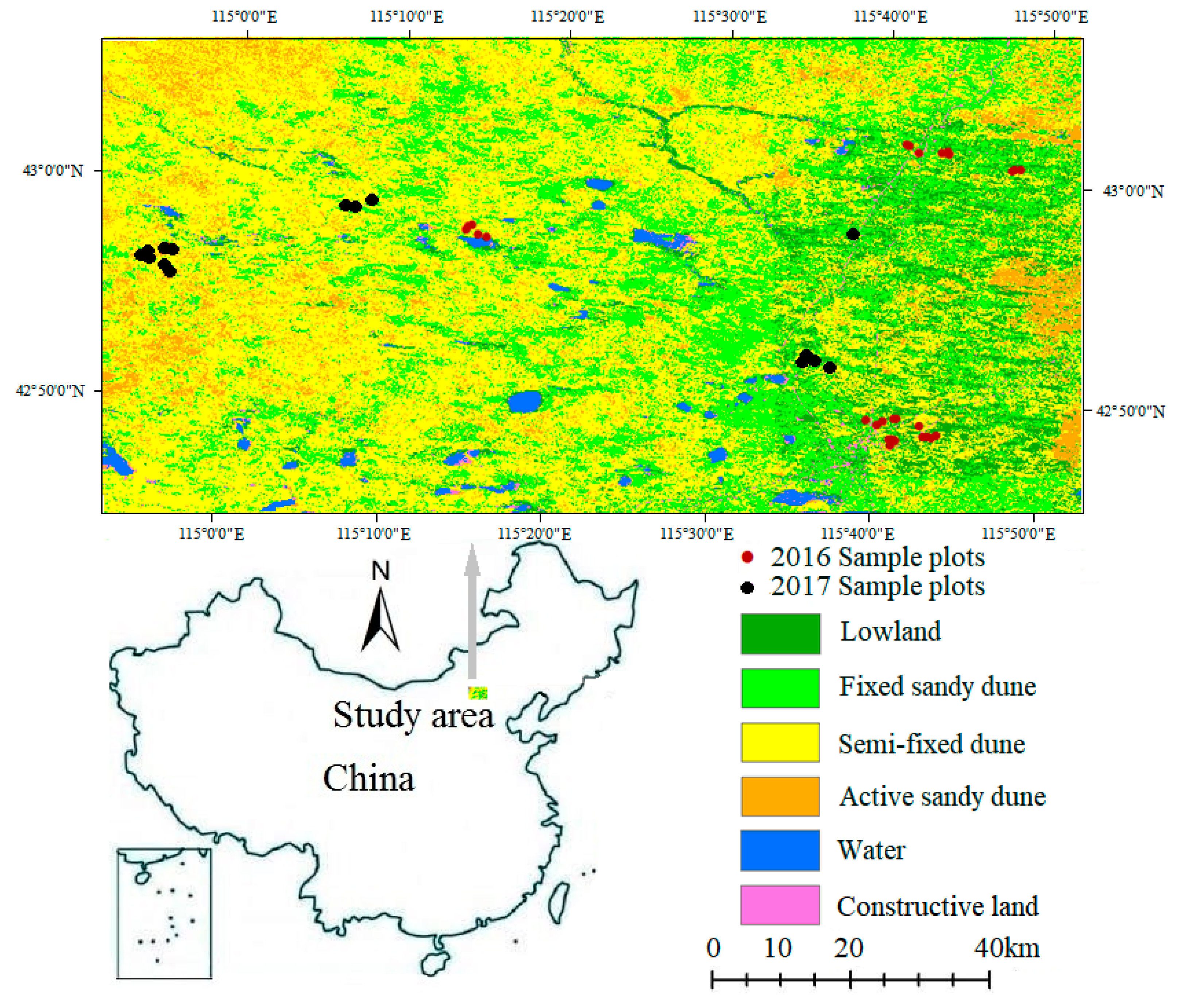
2.1. Study Area

Hunshandak Sandland (41°46′–43°69′N, 114°55′–116°38′E) is one of the four largest sandy temperate grassland areas in China (Figure 1). The prevailing climate is of temperate semi-arid type, with an annual mean temperature of 1.7 °C and a diurnal minimum and maximum monthly temperatures of –18.3 °C and 18.7 °C, respectively. Annual precipitation is 250–350 mm, 80–90% of which falls between May and September. The land cover types of the Hunshandak Sandland include fixed sandy dunes, semi-fixed sandy dunes, active sandy dunes, and low plains that contained rich plant diversity, with the vegetation composition showing small scale variations. These species-rich habitats provide multiple ecosystem services, for example, in preventing the movement of sandy dunes. Therefore, operative schemes for the rapid assessment of fine-scale (0.25–1 m²) plant species diversity are needed to monitor the ecological status in these habitats.

2.2. Plant Diversity Survey and Analysis

We surveyed a total of 270 circular plots, each with a diameter of 0.8m and being randomly distributed throughout the central Hunshandak Sandland. The geographical position of the center was acquired for each sampling plot while using a high-precision hand-hold GPS (UniStrong MG838). The amount, cover, and height of each vascular plant species, and the habitat category of the plot represented (fixed sand dune, semi-fixed sand dune, active sand dune, low elevation plain, water and construction land) were recorded between July and August in either 2016 or 2017. The number of individuals was recorded for the species whose stems were either fully or partially within the subplot. The clonal species were counted as separate individuals, whereas stems or culms grew at distances of more than 20 cm from others specimens of the same species. The same person visually estimated the cover percentage of each species that occurred within the plot for all plots. Polygonum divaricatum was the dominant species in moving dunes; and, Artemisia ordosica dominated at fixed dunes and the low plain. Species richness, which refers to the total number of species per plot, has been widely used as one indicator of plant diversity [30,31]. In our study, species richness atthe plot level was again used as a key indicator of plant biodiversity.

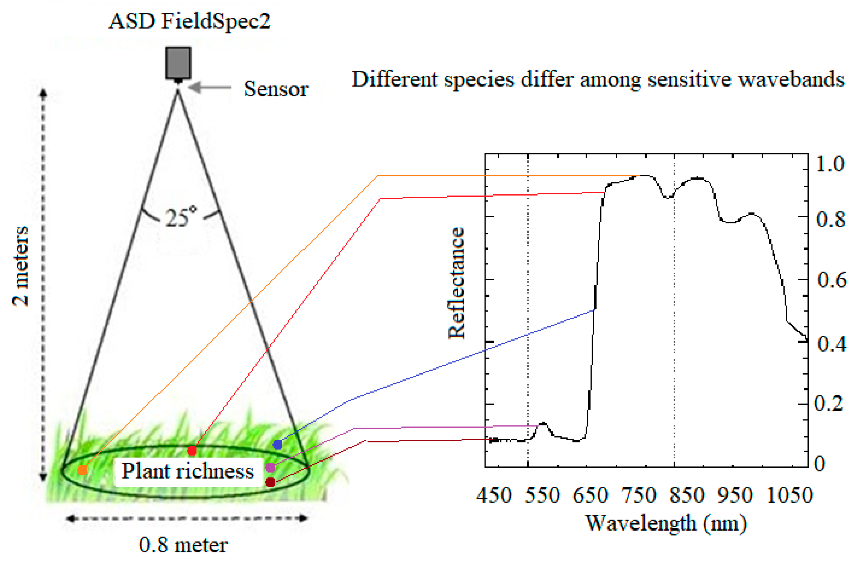
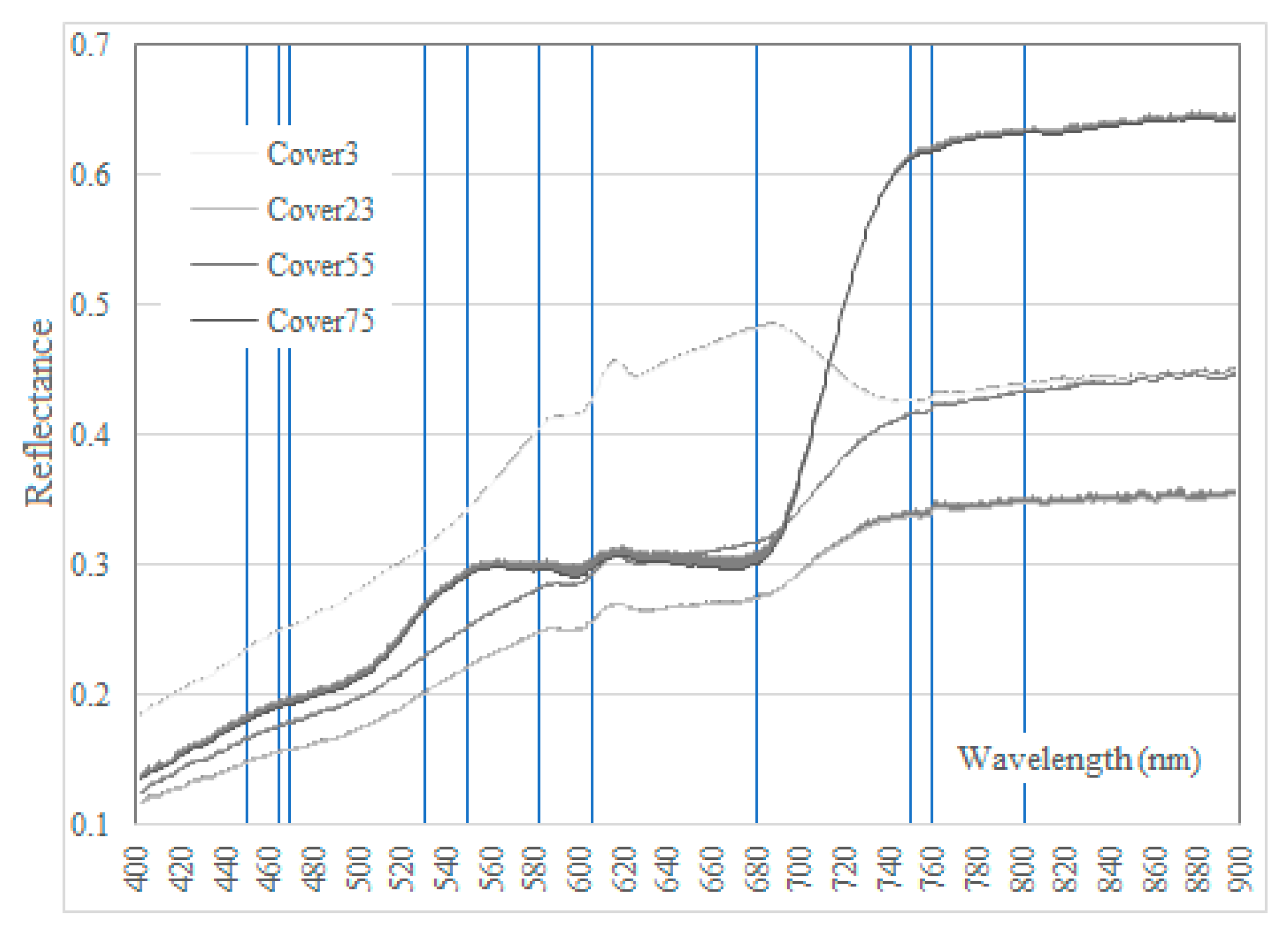
2.3. Hyperspectral Data Measurement and Analysis

Parallel to the vegetation, ground-based hyperspectral measurements were concurrently recorded at each plot using a Hand–Held ASD FieldSpec2 spectrometer (Analytical Spectral Devices Inc., USA). Weighting only 1.2 kg, the spectrometer has a spectral range extending from 325 to 1075 nm and a 1 nm bandwidth (www.asdi.com). Measurements were taken between 10:00–15:00 (Beijing Time) on a sunny windless day. The surveyors dressed in dark and they avoided blocking the sun when measuring in order to minimize environmental reflections. Given the surveyed circle diameter, the canopy reflectance was measured by pointing the fibre optic with a field of view of 25 degrees in a nadir position, located about 2m above the center of each plot, to ensure that only hyperspectral parameters within the surveyed circles were recorded (Figure 2). A white reference panel (spectralon) was used before each spectral measurement to convert spectral radiance into reflectance. Measuring followed the protocol that was used by e.g., [32,33]. Each plot (circle) was measured five times and the averages were calculated across these measurements to account for illumination differences and bi-directional reflectance effects [33]. In the raw data, the marginal ranges 325–374 nm and 1026–1075 nm from each spectrum were removed due to noise effects [34]. Based on Möckel et.al. [28] and our previous studies [29], the sample plots were randomly divided into two datasets: 195 plots were used as training dataset and the remaining 75 plots were used as the validation dataset.

The collected hyperspectral data were preprocessed using the software ViewSpec Pro 6.0 (Analytical Spectral Devices Inc., USA) and then exported into “Statistical Package for the Social Sciences” version 25 (SPSS 25; Chicago, Illinois, USA) to calculate the correlation coefficients and cluster analysis. Figure 3 summaries the work flow of species richness estimation through hyperspectral indices.

2.4. Development Hyperspectral Indices

In this study, we employ a total of 7339 hyperspectral indices (7217 newly developed indices and 122 previously published indices) to identify the best indices in estimating plant species richness. These indices are developed and selected based on SVH through four approaches: (1) combinations of reflectance (Ri) and their first-order derivate values (FD) for each waveband relative to its adjacent waveband; (2) a subset of characterized wavebands (plant absorption peak, reflectance peak, near-, middle-, and edge-spectra in blue, green, and red light); (3) spectral variability indices, i.e., mean (M-), standard deviation (SD-), coefficients of variance (CV), Shannon and Simpson index based on Ri or its FD on the wavebands of (1) and (2); and, (4) empirical spectral indices in previous published literatures.

Combination indices are expressed as Ri or FD at a given wavelength, wavelength difference (Dij), ratio (RR), normalized difference (ND), or inverse reflectance differences (ID) at each waveband and its adjacent waveband (using bands at each 1 nm) in ascending order. Overall, this resulted in ten common types of indices, which are both based on Ri and FD, were used in this study:

Ri

(1)

D = Rj − Ri

(2)

R = Rj/Ri

(3)

ND = (Rj − Ri)/(Rj + Ri)

(4)

ID = 1/Rj − 1/Ri

(5)

FD = FD(Ri)

(6)

FD(D) = FD(Dij) = FD(Rj) − FD(Ri)

(7)

FD(R) = FD(Rj)/FD(Ri)

(8)

FD(ND) = (FD(Rj) − FD(Ri))/(FD(Rj) + FD(Ri))

(9)

FD(ID) = 1/FD(Rj) − 1/FD(Ri)

(10)

where Ri is the mean reflectance, FD is the first-order derivative spectra, and the suffixes (i or j) are wavelengths (nm) of neighboring bands. The FDs were calculated by finite difference approximation. Using this approach, a total of 6500 indices (Ri, D, R, ND, ID; FD, FDD, FDR, FDND, FDID) were created for every waveband or in comparison with two adjacent bands between the ranges of 375–1025 nm (10 × 650 = 6500 indices).

Plant species have distinct physiological traits, demonstrated by their distinct spectral absorption or reflection characteristics in leaves or the plant canopy [35,36,37]. The spectral variability within the individual wavebands can, in this regard, be considered as an indicator of plant species richness. We employed the following specific wavebands that characterize the respective spectral ranges (

Table 1. The specific wavelength ranges of plant biological traits used in the present as potential indicator of plant diversity.

Wavelength Ranges (nm)	Plant Bio-Traits	References
420–440	Chlorophyll-a absorption	[35]
420–480	Chlorophyll absorption	[36]
450–470	Chlorophyll-b absorption	[35]
490–550	Pigment reflected peak	[36]
510–570	Green reflected peak	[36]
630–650	Chlorophyll-b absorption	[35]
630–690	Plant species discrimination	[36]
650–670	Chlorophyll-a absorption	[35]
640–700	Chlorophyll absorption	[37]
673–683	Chlorophyll fluorescence	[37]
680–700	Chlorophyll fluorescence	[37]
720–740	Chlorophyll fluorescence	[37]
700–750	Leaf health and shape	[36]
760–800	Cell structure reflectance peak	[36]
760–900	Discrimination between plant species	[36]
800–960	Species biochemical traits	[36]
900–920	Proteins	[35]
920–940	Oil	[35]
960–980	Starch content, water	[35]
980–1000	Starch content	[35]

), based on the respective literature to extract indicators of plant species diversity.

We calculated the following spectral variability indices at every characterized range as the potential index of plant species richness:

The mean value (M) at each characterized range.

The spectral standard deviation (SD) was used to indicate the spectral heterogeneity within each plot (0.8m-diamater circle) by Formula (11):

$$\mathrm{SD}=\sqrt{\frac{{{\displaystyle \sum }}_{\mathrm{i}=1}^{\mathrm{n}}(\mathrm{Ri}-\mathrm{Rj})}{\mathrm{n}}}$$

(11)

The spectral CV (coefficient of variance, Formula (12)) was used to indicate the spectral heterogeneity within each plot (0.8m-diamater circle) as:

$$\mathrm{CV}=\frac{\mathrm{SD}}{\mathrm{meanR}}$$

(12)

where MeanR is the mean reflectance in a range of wavelength, n is the total number of range bands.

CV increases with increasing spectral variability and is, according the SVH hypothesis, as such, a measure for species richness, which is a common measure of alpha diversity [38].

The spectral Shannon–Wiener index was calculated as [29]:

$$\mathrm{ShannonRi}=-{{\displaystyle \sum }}_{\mathrm{i}=1}^{\mathrm{n}}\frac{\mathrm{Ri}}{\mathrm{Rn}}\ln \frac{\mathrm{Ri}}{\mathrm{Rn}}$$

(13)

where ShannonRi is the spectral diversity in a circle of n bands, Ri is the reflectance value of the ith band, Rn is the total number of bands, and ln is the natural logarithm. The higher value of Hs means higher spectral diversity and hence greater plant diversity. The band unit (n) also indicated various spectral regions (in Table 1), which aimed to find the best ShannonRi.

The Simpson spectral evenness index (SimpsonRi) was calculated as [29]:

$$\mathrm{SimpsonRi}=1-{{\displaystyle \sum }}_{\mathrm{i}=1}^{\mathrm{n}}{(\frac{\mathrm{Ri}}{\mathrm{Rn}})}^2$$

(14)

The values of the Simpson spectral evenness index range from 0 (completely uneven) to 1 (different reflectances occur in equal numbers). The meaning of Ri, Rn, and n are the same as in Formula (13). Simpson’s evenness values were also calculated at all, specific, and every individual band, as in Formula (13).

SD and CV were calculated for D, R, ND, ID, FD, FDD, FDR, FDND, and FDID on the whole range of 375–1025 nm, respectively; M, SD, CV were calculated on Ri, D, R, ND, ID, FD, FDD, FDR, FDND and FDID on each characterized range in Table 1; and, Shannon and Simpson indices on Ri and FD for each characterized range are shown in Table 1. This resulted in a total of 713 additional indices (2 × 9 = 18 indices for a range of 375–1025 nm; 3 × 10 × 20 = 600 indices for 20 ranges in Table 1; 15 absolute values for CV; and, 2 × 2 × 20 = 80 indices for Shannon–Wiener and Simpson index).

SD, CV, Shannon, and Simpson indices on 20 characterized ranges (Table 1) (four indices).

Totally: 713 + 4 = 717 indices.

We also employed 122 spectral indices (Appendix A,

Table A1. The published empirical spectral indices [24,34,38,39,40] used for estimating plant species richness in Hunshandak Sandland, China.

Index1	$\frac{R_{800}}{R_{680}}$	Index62	$\frac{R_{728}-R_{434}}{R_{720}-R_{434}}$
Index2	$\frac{R_{800}}{R_{650}}$	Index63	$\frac{R_{782}-R_{675}}{R_{782}+R_{675}}$
Index3	$\frac{R_{800}}{R_{550}}$	Index64	$\frac{R_{865}-R_{672}}{R_{865}+R_{672}}$
Index4	$\frac{R_{750}}{R_{700}}$	Index65	$\frac{R_{800}-R_{670}}{R_{800}+R_{670}}$
Index5	$\frac{R_{750}}{R_{550}}$	Index66	$\frac{R_{800}-R_{635}}{R_{800}+R_{635}}$
Index6	$\frac{R_{740}}{R_{720}}$	Index67	$\frac{R_{774}-R_{677}}{R_{774}+R_{677}}$
Index7	$\frac{R_{725}}{R_{702}}$	Index68	$\frac{R_{750}-R_{705}}{R_{750}+R_{705}}$
Index8	$\frac{R_{710}}{R_{760}}$	Index69	$\frac{R_{750}-R_{550}}{R_{750}+R_{550}}$
Index9	$\frac{R_{705}}{R_{722}}$	Index70	$\frac{R_{570}-R_{670}}{R_{570}+R_{670}}$
Index10	$\frac{R_{700}}{R_{670}}$	Index71	$\frac{R_{531}-R_{570}}{R_{531}+R_{570}}$
Index11	$\frac{R_{695}}{R_{670}}$	Index72	$\frac{R_{557}-R_{643}}{R_{557}+R_{643}-R_{465}}$
Index12	$\frac{R_{695}}{R_{760}}$	Index73	$\frac{R_{728}-R_{720}}{R_{728}+R_{720}-2\ast R_{434}}$
Index13	$\frac{R_{695}}{R_{420}}$	Index74	$\frac{1}{R_{695}-R_{705}}-\frac{1}{R_{750}-R_{800}}$
Index14	$\frac{R_{672}}{R_{550}}$	Index75	$\frac{R_{750}-R_{706}}{R_{750}+R_{706}-2\ast R_{445}}$
Index15	$\frac{R_{657}}{R_{700}}$	Index76	$\frac{\frac{R_{800}}{R_{670}}-1}{{(\frac{R_{800}}{R_{670}}+1)}^{\frac{1}{2}}}$
Index16	$\frac{R_{630}}{R_{680}}$	Index77	$\frac{\frac{R_{750}}{R_{705}}-1}{{(\frac{R_{750}}{R_{705}}+1)}^{\frac{1}{2}}}$
Index17	$\frac{R_{605}}{R_{760}}$	Index78	$(1+0.45)\ast \frac{Rn2+1}{Rr+0.45}$
Index18	$\frac{R_{600}}{R_{680}}$	Index79	$\frac{R_{750}-R_{705}}{R_{750}+R_{705}-2\ast R_{445}}$
Index19	$\frac{R_{430}}{R_{680}}$	Index80	$2.5\ast \frac{R_{782}-R_{675}}{R_{782}+6\ast R_{675}-7.5\ast R_{445}+1}$
Index20	$\frac{R_{715}}{R_{705}}$	Index81	[(R700 − R672) − 0.2 ∗ (R700 − R553)]
Index21	$\frac{R_{725}}{R_{702}}$	Index82	[(R700 − R672) − 0.2 ∗ (R700 − R553)] ∗ (R700/R672)
Index22	$\frac{R_{900}}{R_{970}}$	Index83	((R782 − R675)/(R782 + R675 + 0.2)) (1.2)
Index23	$\frac{R_{690}}{R_{550}}$	Index84	0.5(R782 − 0.5R675 − 0.2)/(0.5R782 + 0.5R675 − 0.1)
Index24	$\frac{R_{675}}{R_{782}}$	Index85	$2\ast R_{800}+1-{(2\ast R_{800}+1)}^2-8\ast (R_{800}-R_{670}){)}^{\frac{1}{2}}$
Index25	$\frac{R_{810}}{R_{660}}$	Index86	($R_{800}-0.2R_{670}-0.6$)/1.019
Index26	$\frac{R_{680}}{R_{550}\ast R_{708}}$	Index87	2.5 × ((R865 − R672)/(R865 + 6 × R672 − 7.5 × R465 + 1))
Index27	$\frac{R_{675}}{R_{700}\ast R_{650}}$	Index88	$((R_{750}-R_{705})-0.2\ast (R_{750}-R_{550}))(\frac{R_{750}}{R_{705}})$
Index28	$\frac{R_{672}}{R_{550}\ast R_{708}}$	Index89	R700 + 40[(R670 + R780)/2 − R700 ]/(R740 − R700)
Index29 RDVI	(R800 − R670)/sqrt(R800 + R670)	Index90	(1 + 0.16)( R800 − R670)/( R800 + R670 + 0.16)
Index30 MSR	(R800/R670 − 1)/sqrt(R800/R670 + 1)	Index91 MCARI	$((R_{700}-R_{670})-0.2(R_{700}-R_{550}))(\frac{R_{700}}{R_{670}})$
Index31 MCARI1	1.2[2.5(R800 − R670) − 1.3(R800 − R550)]	Index92 $TCARI$	$3\ast ((R_{700}-R_{670})-0.2\ast (R_{700}-R_{550})\ast (\frac{R_{700}}{R_{670}})$
Index32 MTVI1	1.2[1.2(R800 − R550) − 2.5(R670 − R550)]	Index93 $OSAVI1$	$\frac{(1+L)(R_{800}-R_{670})}{R_{800}+R_{670}+L},\mathrm{L}=0.16$
Index33 TVI	0.5(120*(R750 − R550) − 200(R670 − R550))	Index94 $OSAVI2$	$\frac{(1+L)(R_{800}-R_{670})}{R_{800}+R_{670}+L},\mathrm{L}=0.5$
Index34	$LN(\frac{1}{R_{737}})$	Index95 $OSAVI3$	$\frac{(1+L)(R_{800}-R_{670})}{R_{800}+R_{670}+L},\mathrm{L}=0.2$
Index35	$\frac{1}{R_{510}}-\frac{1}{R_{550}}$	Index96	$\frac{TCARI}{OSAVI1},L=0.16$
Index36	$\frac{1}{R_{510}}-\frac{1}{R_{700}}$	Index97	$\frac{TCARI}{OSAVI2},L=0.5$
Index37	$\frac{1}{R_{553}}-\frac{1}{R_{700}}$	Index98	$\frac{TCARI}{OSAVI3},L=0.2$
Index38	$\frac{1}{R_{511}}-\frac{1}{R_{553}}$	Index99	$0.5\ast [2\ast R_{800}+1-{({(2\ast R_{800}+1)}^2-4\ast (R_{800}-R_{670}))}^{\frac{1}{2}}]$
Index39	$\frac{1}{R_{511}}-\frac{1}{R_{700}}$	Index100	$$\begin{gathered} (1.5\ast (2.5\ast (R_{800}-R_{670})-1.3\ast (R_{800}-R_{550}))) \\ /sqrt({(2\ast R_{800}+1)}^2-(6\ast R_{800}-5\ast sqrt(1.5\ast (2.5\ast (R_{800}-R_{670})-1.3 \\ \ast (R_{800}-R_{550})))/sqrt({(2\ast R_{800}+1)}^2 \\ -(6\ast R_{800}-5\ast sqrt(R_{670}))-0.5) \end{gathered}$$
Index40	$R_{800}\ast (\frac{1}{R_{500}}-\frac{1}{R_{700}})$	Index101	Mean (R500 to R600)
Index41	$R_{800}-R_{550}$	Index102	MeanRed (600–699 nm)/mean Green (500–599 nm)
Index42	$R_{810}-R_{680}$	Index103	(Max first derivative: 680–750 nm)
Index43	$\frac{R_{680}-R_{500}}{R_{750}}$	Index104	The highest first derivative value between 490–530 nm (Db)
Index44	$\frac{R_{681}-R_{502}}{R_{753}}$	Index105	The highest first derivative value between 550–580 nm (Dg)
Index45	$\frac{R_{680}-R_{550}}{R_{750}}$	Index106	The highest first derivative value between 680–780 nm (DR)
Index46	$\frac{R_{800}-R_{680}}{R_{800}+R_{680}}$	Index107	The highest first derivative between 510–580 nm (Rg)
Index47	$\frac{R_{557}-R_{643}}{R_{557}+R_{464}}$	Index108	The smallest reflectance value between 640–700 nm (Ro)
Index48	$\frac{R_{802}-R_{465}}{R_{802}+R_{681}}$	Index109	The sum of first derivative values between 490–530 nm (SDb)
Index49	$\frac{R_{802}-R_{676}}{R_{800}+R_{676}}$	Index110	The sum of first derivative values between 550–580 nm (SDg)
Index50	$\frac{R_{550}-R_{450}}{R_{550}+R_{450}}$	Index111	The sum of first derivative values between 680–780 nm (SDR)
Index51	$\frac{R_{415}-R_{435}}{R_{415}+R_{435}}$	Index112	Rg/Ro
Index52	$\frac{R_{722}-R_{700}}{R_{722}+R_{700}}$	Index113	(Rg − Ro)/(Rg + Ro)
Index53	$\frac{R_{722}-R_{502}}{R_{700}-R_{502}}$	Index114	SDR/SDb
Index54	$\frac{R_{850}-R_{710}}{R_{850}-R_{680}}$	Index115	SDR/SDg
Index55	$\frac{R_{780}-R_{710}}{R_{780}-R_{680}}$	Index116	(SDR − SDb)/(SDR + SDb)
Index56	$\frac{R_{800}-R_{445}}{R_{800}-R_{680}}$	Index117 MCARI2	1.5*(2.5(R800 − R670) − 1.3(R800 − R550))/sqrt((2R800 + 1)^2 − (6R800 − 5*sqrtR670) − 0.5)
Index57	$\frac{R_{750}-R_{445}}{R_{705}-R_{445}}$	Index118 MTVI2	1.5*(1.2*(R800 − R550) − 2.5*(R670 − R550))/sqrt((2*R800 + 1)^2 − (6*R800 − 5*sqrtR670)) − 0.5)
Index58	$\frac{R_{734}-R_{747}}{R_{715}-R_{720}}$	Index119 CARI	(|670*(R700 − R550)/150 + R670 + R550 − 3.67*(R700 − R550)|/sqrt(((R700 − R550)/150)^2 + 1))*R700/R670
Index59	$\frac{R_{734}-R_{747}}{R_{715}+R_{726}}$	Index120 MSAVI	$0.5\ast [2\ast \mathrm{Mean}(\mathrm{R}760~\mathrm{R}960)+1$ $-({(2\ast \mathrm{Mean}(\mathrm{R}760~\mathrm{R}960)+1)}^2-8$ $\ast \mathrm{Mean}(\mathrm{R}760~\mathrm{R}960)$ ${-\mathrm{Mean}(\mathrm{R}660~\mathrm{R}760))}^{\frac{1}{2}}]$
Index60	$\frac{R_{753}-R_{700}}{R_{753}+R_{700}}$	Index121 NDVI	(mean($\mathrm{R}760~\mathrm{R}960$) − mean(R660~R760))/(mean($\mathrm{R}760~\mathrm{R}960$) + mean($\mathrm{R}660~\mathrm{R}760$))
Index61	$\frac{R_{534}-R_{572}}{R_{534}+R_{572}}$	Index122 SAVI	1.5*(mean($\mathrm{R}760~\mathrm{R}960$) − mean(R660~R760))/(mean(R760~R960) + mean($\mathrm{R}660~\mathrm{R}760$)+0.5)

) that were published in previous studies, which served as reference [24,34,38,39,40]. This means that the total number of indices tested was 7339 (6500 + 717 + 122 = 7339).

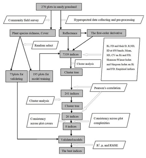
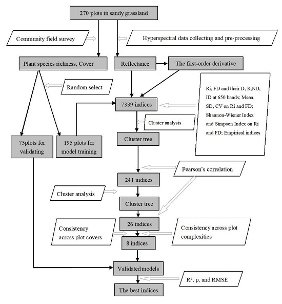
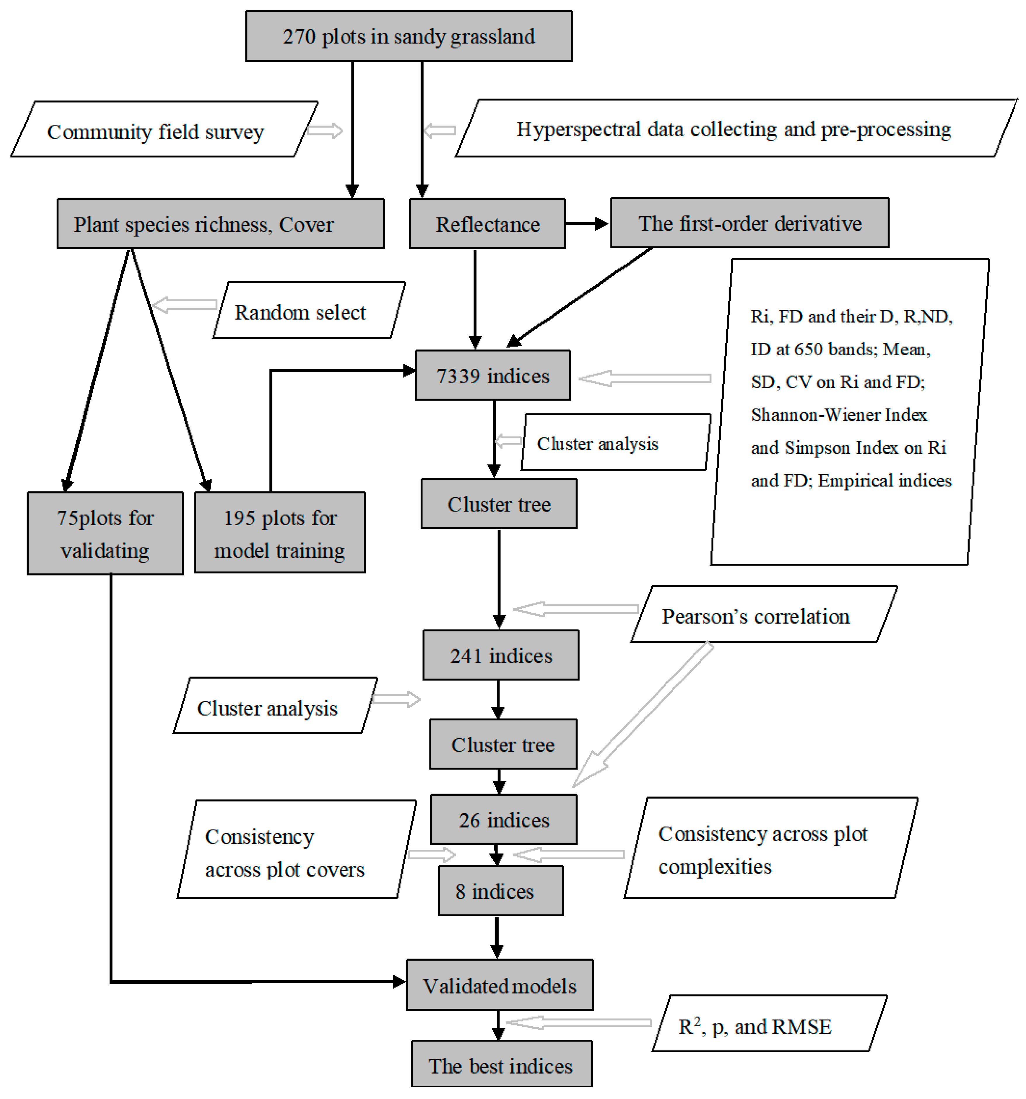
2.5. The Method for Identification of the Best Indices

One of the key aims of our study was to identify the best spectral indices to predict plant species richness. This identification was mainly based on correlation analysis, cluster analysis, and model validation. Indices were considered to be optimal when they were statistically significantly (p < 0.05) linked to plant species richness based on Pearson’s correlation analysis [41]. Within the group of significant predictors, the indices with the highest coefficients of determination (R²) that were obtained through linear modelling would be selected as potentially “best” predictors. However, many indices showed very similar, strong relationship with species richness. Therefore, we used a cluster analysis to select the most significant indices within each similar-performing group, deleting the redundant collinear spectral indices to narrow down the number of selected indices. Therefore, the purpose of the cluster analysis was to identify the indices showing very similar associations with plant diversity, hence being closely associated with each other [42]. Overall, the identification of similarity was based on (1) the determination of shared commonalities in accuracy and similar content in indices and (2) by the division of indices into various groups [43]. These groups were not known prior to conducting the mathematical analysis and no a priory assumption were made regarding the distribution of variables (indices). The indices were also z-transformed for the analysis. The results are presented in a dendrogram with groupings based on a squared Euclidean distance matrix. Following cluster analysis, only indices that have significant correlation coefficients, representing the group which they belong to, were used for further analysis as representatives of their respective groups.

The potential spectral indices should be highly consistent in predicting plant species richness across different plant communities. We used two types of community conditions to test how they influence the consistency of the selected indices in estimating the richness of plant species in the proposed indices. First, % cover was regarded as one important factor that potentially affects species richness predictions [44]. Second, species richness is a common indicator of community complexity [45], also due to different species generally varying in their morphological traits. These two conditions were separated into three classes based on values: 0–25, 26–40, and 40–100%, therefore representing low, moderate, and high % cover of the community and 1–3, 4–6, and 7–12 (species richness) as low, moderate, and high community complexity, respectively.

The indices that were retained after these steps were selected as final target indices if they also passed the validation test. For this test, we used the remaining 75 plots that were randomly selected for model validation. The performance of the proposed indices in the validating test was assessed using four variables that were obtained in the validated datasets: the coefficient of determination (R² and adjusted R², calculated by linear modelling), the root mean square error (RMSE), and the significance level (p) between the predicted and observed richness values. High values of R² and low values of RMSE indicate high model quality. The indices that had the highest adjusted R² and the lowest RMSE with a p < 0.01 were considered as to be the best predictor [46]. The RMSE was calculated using the following formula:

$$\mathrm{RMSE}=\sqrt{\frac{{{\displaystyle \sum }}_{\mathrm{j}=1}^{\mathrm{n}}(\mathrm{yj}-\widehat{\mathrm{y}}\mathrm{j})2}{\mathrm{n}}}$$

(15)

where, y = observed species richness value, ŷ = estimated species richness value, and n = number of sample plots.

3. Results

3.1. Cluster trees in two stages

The spectral indices clustered into five distinct groups (positive and negative significant relation at 0.01 and 0.05 level, respectively, and a non-significant relation) in the hierarchical cluster tree based on all 7339 hyperspectral indices (Figure S1). These results (see also relations Table S1 in Supplementary Data) suggest a strong degree of consistency in the selection of desirable indices as a basis cluster to select the best indices. The positive significant indices mostly occurred in the spectra between 500–800 nm, as demonstrated by FD, R, D, ND or SD, and CV. The Ri indices in the range between 400–900 nm commonly showed mostly negative correlations with plant species richness. The indices in these groups have the best potential as indicators of plant species richness. We chose 241 indices in the characterized groups for further investigation.

These 241 indices were clustered to identify the best index ranges. The resultant dendrogram tree (Figure S2 in Supplementary Data) indicates that the indices that are strongly aligned with plant species richness are closely associated. We first selected the closest indices using the Pearson’s correlation coefficients (Table S2 in the Supplementary Data), followed by a browsing cluster dendrogram (Figure S2), in order to discern their location in the tree one-by-one, with most representatives found near the center of the selected group. Using this approach, the most sensitive 26 indices were selected as the potential best indices for further analysis. Additionally, they also had significantly higher Pearson’s correlation coefficients with plant species richness per plot (|r| > 0.5) than the other tested indices.

3.2. Performance Under Different Community Conditions

The selected 26 spectral indices were compared regarding their consistency of relation to species richness for different community conditions.

Table 2. Correlation coefficients between the hyperspectral indices and field-measured species richness displayed with their variation across community covers and complexities. Bold letters indicate significance at the 0.05 level.

Hyperspectral Indices	R2 (n = 195)	Cover (n = 65)			Complexity (n = 65)
		L	M	H	L	M	H
R583	0.284	−0.611	−0.509	−0.424	−0.552	−0.222	0.181
SDFD420-480	0.340	−0.623	−0.474	−0.351	−0.410	−0.162	0.203
SDFD450-470	0.310	0.660	0.281	0.387	0.381	0.379	−0.234
D604	0.298	−0.671	−0.338	−0.293	−0.407	−0.081	0.111
FD603	0.275	−0.401	−0.727	−0.395	−0.268	−0.073	−0.176
FD606	0.275	−0.335	−0.580	−0.582	−0.561	−0.333	−0.319
FD437	0.327	−0.293	−0.572	−0.427	−0.301	−0.341	−0.058
FD490	0.325	−0.279	−0.546	−0.399	−0.534	−0.210	−0.027
SD-D420-480	0.278	−0.585	−0.476	−0.412	−0.566	−0.620	0.177
SD-D450-470	0.267	−0.532	−0.413	−0.382	−0.581	−0.310	−0.090
FD460	0.283	−0.573	−0.451	−0.313	−0.379	−0.232	0.237
FD583	0.283	−0.606	−0.325	−0.462	−0.592	−0.264	0.402
D583	0.329	−0.629	0.005	−0.486	−0.486	−0.195	−0.135
MeanFD450-470	0.275	0.551	0.156	0.475	0.273	−0.005	0.277
SD450-470	0.295	−0.476	−0.505	−0.466	−0.680	−0.405	0.365
FD497	0.292	−0.396	−0.544	−0.317	−0.436	−0.087	0.040
FD403	0.354	−0.395	−0.528	−0.279	−0.455	−0.125	0.219
FD531	0.279	−0.455	−0.465	−0.428	−0.686	−0.391	0.400
ND528	0.264	−0.598	−0.464	−0.499	−0.513	−0.051	0.132
R528	0.263	−0.525	−0.553	−0.612	−0.484	−0.058	−0.170
FDD588	0.260	0.358	0.455	0.378	0.285	−0.003	0.216
ShannonFD760-900	0.258	0.409	0.358	0.313	0.474	0.333	−0.390
Index48	0.211	0.408	0.368	0.332	0.452	0.395	−0.361
Index69	0.218	0.477	0.394	0.254	0.495	0.326	−0.379
Index78	0.231	0.505	0.399	0.267	0.502	0.307	−0.413
Index121	0.238	−0.611	−0.509	−0.424	−0.552	−0.222	0.181

lists the Pearson’s correlation coefficients between the hyperspectral indices and species richness at the three degrees of community cover (L, Low, <25%; M, Moderate, 26–40%; H, High, >40%) and community complexity (L, Low, 1–3; M, Moderate, 4–6; H, High, >7). The indices that showed significant correlations for all different community conditions were chosen as the potential best indices.

Table 2 shows that the indices were significantly related to species richness under different community covers, yet are varied with high community complexity. The indices FD531, FD583, FD606, SD450–470, ShannonFD760–900, Index48, Index69, and Index78 were significantly related to species richness under different community conditions.

Regarding the effects of community cover, the reflectance of a community may proportionally relate to the community cover. We examined the performance of the spectral curves with the same species richness under four cover conditions (Figure 4). These plots were chiefly covered by the three-herb species: Artemisia desertorum, Artemisia intramongolica, and Agriophyllum squarrosum. For the plots with a cover of 3%, where the majority of the ground was covered by sandy soil without vegetation, the reflectance curve contained strong non-vegetation signal. For plots with covers of 23, 55 and 75%, the curves were increasingly characterizing the distinct vegetation trait of the respective community. The differences in the curves were mainly at the edge of red light (520–600 nm) and near infrared red (720–900 nm). In these spectral ranges, the standard deviations also peaked. Based on Figure 4, it can be deduced that the changes in reflectance are not directly proportional to the changes in community cover. The FD at the sensitive bands of 531, 583, and 606 nm remains almost stable, although high variation existed in the original reflectance. It was also observed that the same standard deviation for reflectance from 450–470 nm occurred under four cover conditions. The Shannon–Wiener Index on FD in the range of 760–900 nm, within the near-infrared near region, also maintained similar values, indicating stable species richness across plots.

The eight spectral indices that passed the above-mentioned tests were retained for model development. The established models showed a high determination coefficient (R²), significant relationship between index and plant species richness (p < 0.05), and low RMSE (

Table 3. Selected hyperspectral indices, models, and parameters in estimating plant species richness based on the training dataset.

The Indices	The Models	R2	p	RMSE
FD606	Y = 5.691 − 1188.364x	0.271	<0.001	1.839
FD583	Y = 5.609 − 1999.106x	0.279	<0.001	1.828
FD531	Y = 8.861 − 3241.099x	0.276	<0.001	1.833
SD450-470	Y = 7.043 − 857.869x	0.291	<0.001	1.813
ShannFD760-900	Y = 2.256x − 3.402	0.254	<0.001	1.860
Index48	Y = 1.776 + 6.17x	0.207	<0.001	1.918
Index69	Y = 2.18 + 7.024x	0.214	<0.001	1.909
Index78	Y = 3.827x − 4.641	0.227	<0.001	1.893

), demonstrating them to be potentially best indices.

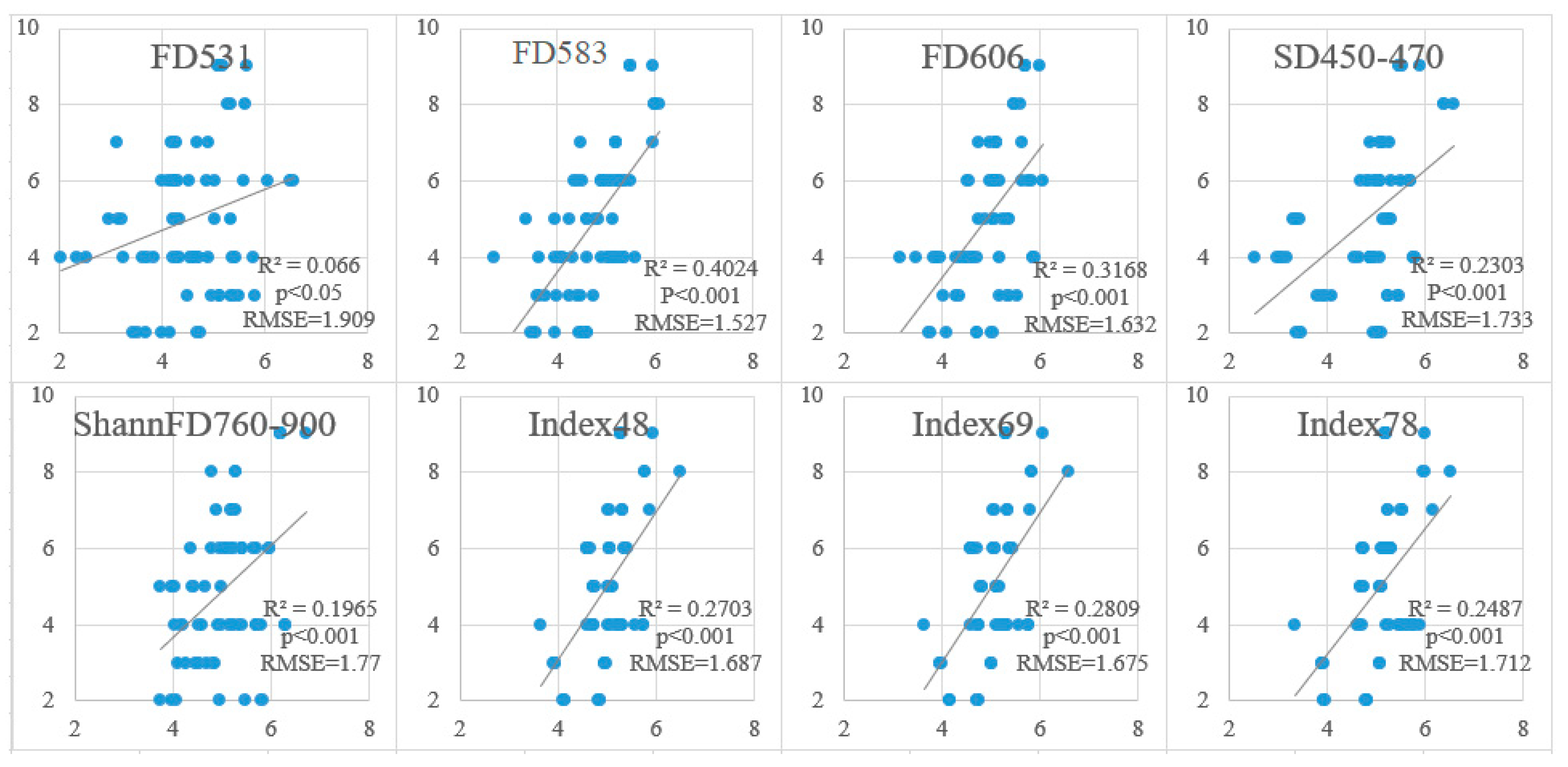
3.3. Validation of Proposed Models

Based on the eight identified best hyperspectral indices that are listed in Table 3, plant richness was calculated using the hyperspectral dataset collected at the 75 model validation plots. The linear correlation between the estimated diversity using hyperspectral indices and the field-survey plant diversity was analyzed at the plot level (Figure 5). All of the models showed a significant correlation (p < 0.05) between recorded and predicted species richness. By comparing the R², all of the hyperspectral models showed similarly high values (R² > 0.2), with the exception of FD531. The RMSE ranged from 1.5 to 1.9, and FD583, FD606, (R802 − R465)/(R802 + R681), and (R750 − R550)/(R750 + R550) were the best predictors within the set of indices that were distilled by the previous analysis.

4. Discussion

4.1. Fit. to SVH

In the present study, we tested the suitability of the spectral traits as plant diversity indices, i.e., looking as the standard deviation (SD), coefficients of variance (CVs), and the Shannon and Simpson indices of original reflectance or its FD, on the wavebands of all wavelengths of hyperspectral plot data to test their ability to predict plant species richness. Most of the indices were significantly related to species richness, with ShannonFD760–900, SD-FD420–480, SD-FD450–470, SD-FDD490–550, and SD450–470 displaying the strongest links. These results indicated that the variability within the visible region of the electromagnetic spectrum (~420–470 and 490–550 nm) and near-infrared region (760–900 nm) can effectively indicate species richness. The number of spectral indices that were significantly related to species richness on the bands in the visible range (~420–550 nm) was greater than those in the NIR range (~760–900 nm). Similar results were observed and reported in a previous study of prairie species richness [31]. Spectral differences related to the diversity in pigment content [35,36], water content, structural elements, cell size, intercellular space, and cell wall thickness can assist in differentiating among plant species and communities [5,47,48]. Wavebands that characterize these plant physiological and structure traits were employed in our study (Table 1) to extract plant diversity information [4,35,47]. The results support the hypothesis that the spectral variability that was recorded between communities can capture key information showing the occurrence of different plant species [49,50], i.e., reflecting plant species diversity. This is an important result as collecting leaf spectra (mainly canopy spectra for herb and grass communities) is much more time efficient than traditional approaches (community survey) and it allows for repeated sampling of the same plots over years.

However, not all of the spectral diversity indices were significantly related to species richness. In the present study, spectral variability indices (the SD, CV, Shannon–Wiener, and Simpson indices on Ri and its FD on entire wavebands) failed to predict species diversity. For entire wavebands in the sparse vegetation of sand dunes, the spectral signs that were recorded by a handheld instrument represent a mixture of vegetation and sand dune reflectance. Sand dunes strongly affect these mixed signs, because the community cover of most plots ranged between 25 and 55%, with barren sand dunes occupying a significant part of the plot [51]. Sandy soils have a stronger reflectance than vegetation in the visible spectral range [35,47]. The failure to detect a significant relationship between spectral variation and species diversity in some of the investigated indices might be related to the entropy index being calculated by all of the selected bands for 380–1025 nm, rather than for red and NIR bands, separately. Thus, the spectral entropy primarily reflected the information of entire plots (i.e., vegetation and non -vegetated area) within plots, rather than the variation among various plant species. Therefore, some spectral diversity indices mostly reflect the traits of a mixture of vegetation, sand dunes, and vegetation shadows, rather than the community composition, as already reported in a previous study of species alpha diversity indices from the same area [29].

The FD is a significant indicator of the degree of deviation for reflectance across neighboring bands; it has been used to reduce the variation in spectral reflectance, because of surface geometry, roughness, and the effects of water absorption features on the spectrum [52]. Moreover, FD has the potential to eliminate the background signals and overlapping spectral features. In the current study, the FD models were very effective in approximating plant species diversity, particularly in linear stepwise regression models. Significant variation in the reflectance of the sensitive bands might partially explain this high estimation accuracy. FD has also been extensively used in numerous models for estimating vegetation parameters that have highlighted a significant advance in model accuracy when compared to other indices [29,53]. It is apparent that the selection of sensitive bands by correlation and cluster analysis can greatly improve the predictive performance of FD for plant diversity. Therefore, it is not surprising that first-order derivate values of reflectance, particularly for the bands of 531, 583, and 606 nm, within the visible range, were strongly linked to plant species richness in our study. The same performance was also observed for the expanded indices of ND (465, 681, and 802 nm and 550 and 750 nm). These results indicate that, other than spectral diversity indices, the deviation values and normalized difference indices of sensitive wavebands can be used as accurate predictors of plant species richness. In summary, spectral diversity and normalized difference indices within the visible (420–550 nm) and NIR (760–900 nm) ranges, rather than the entire range, are substantial indicators in predicting species richness.

4.2. Methods Used to Identify the Best Indices

The most sensitive wavelengths, selected via the correlation and cluster analysis, were 465, 531, 550, 583, 606, 681, and 750 nm, and the spectral ranges of 420–480, 450–470, and 760–900 nm. The selected spectral ranges were represented, because we identified the candidate wavebands through correlation and cluster analysis that were based on the entire spectral indices from 375 to 1025 nm. Cluster analysis has an advantage in showing a high degree of dissimilarity between groups that were derived from the hyperspectral indices based on entire wavebands (375–1025 nm). The best potential indices regarding species richness in this approach are assumed to cluster together, because they all extract the same key information from hyperspectral data [43]. The best-performing indices within each group can then be selected as representing the group’s characteristics [42], thus making it easy to select the best potential indices and avoiding redundancy in the selection from 7339 indices.

In the first cluster tree of 7339 indices, there are three obvious cluster groups. The spectral variation indices (SD and CV) in the ranges of 420–480, 450–470, and 420–550 nm was clustered together, and FDs from 400 to 550 nm, RIs from 380 to 620 nm, and the Shannon–Wiener index for FDs from 760–900 nm were clustered together, respectively (Figures S1 and S2). The other indices were scattered in many small groups in the cluster tree. The bands of 465, 531, 550, 583, 606, 681, and 750 nm demonstrated a particularly strong role in each small group. In the second cluster tree, 241 indices were clustered into two main groups with five sub-groups, with each group reflecting the statistical similarity and the spectral traits regarding species diversity.

The special wavelengths that were selected using cluster analysis in our study also demonstrated biological features with regards to plant species diversity. The wavelengths from 420 to 480 nm, and particularly between 450 and 470 nm, lie in the visible range, and are often strongly absorbed by plant chlorophyll and carotenoids in green plants [54,55]. The reflectance values at 465 nm (within the range of 420–480 nm) and 583 nm indicate the contents of carotenoids and chlorophyll, while the 531 nm wavelength mainly indicates anthocyanins, rather than carotenoids and chlorophylls. Chlorophyll b is indicated at the wavelengths that are near 681 nm [48]. The wavelengths of 606, 681, and 750 nm are sensitive indicators of leaf nitrogen contents (LNC) and chlorophyll [56]. A wavelength at 750 nm is a better indicator to estimate chlorophyll content, because it is less affected by leaf and canopy structure [57]. The near-infrared bands, such as bands between 760 and 900 nm, have been used to assess leaf structure [48]. Contents of chlorophyll, carotenoids, anthocyanins, and proteins in leaves, and the leaf structure of green plants, are the key information reflecting variations different plant species [58]. Consequently, the variability in these biologically characterized wavebands successfully indicated species variability among communities in our study. For indices that are within the NIR range, studies have reported the possible links between certain components in the leaves, like proteins and cellulose, and the leaves’ NIR properties. Nonetheless, their impact on the variability of leaf spectra appears less pronounced when compared to specific pigments (with reflectance in the visible range) [47]. This may partly explain the low accuracy of NIR indices; with only the Shannon–Wiener index on FD from 760–900 nm was selected after the two steps of cluster analysis.

4.3. Accuracy, Stability and Complexity

The best model should have good precision, high stability, short running time, and a low level of operational complexity. Although some studies have reported that stepwise multiple linear regression (SMLR), partial least square regression (PLSR), and support vector machine regression (SVR) can obtain high prediction accuracy, such results were obtained at the expense of increasing model complexity, because of the use of whole set of wavebands (more than 200 variables) for modeling [29,59]. Acquiring optimal models from these reflectances across more than 200 wavebands from hyperspectral imageries not only requires measurements of a large number of standardized samples, but also an intensive data pre-processing, which may lead to problems of regarding cost and efficiency. Therefore, multivariate regression-based indicators are problematic in terms of their balance between model accuracy and simplicity [59]. In contrast, the spectral indices based on narrow wavebands that can be clearly linked to biological features that are characterized by various plant species, such as the proposed indices in the present study, can capture key information in the reflectance variation among the plant species. Therefore, these models are simpler to process and they hence have the advantages of relying on time-efficient field measurements.

To identify the most sensitive wavebands and their best combinations, we developed more than 7000 indices that were based on reflectance or its FD for every waveband, and their complete combinations on entire wavebands, and characterized 20 ranges. Correlation coefficients, significance level, and RMSE are usually used to evaluate the prediction accuracy of statistical models [59,60], the consistency under community conditions, and model complexity by the number and collinearity of the variables in the models. Our study considered all of these important parameters.

We also used variations in community covers and complexity to test the stability of the selected spectral indices. The influences of the community conditions of cover and complexity are problems that are frequently encountered in remote sensing approaches targeting the prediction of plant diversity [25,41,44]. Sandy grassland is often associated with a low community cover and a higher plant species richness [61,62]. Soil background and differences in soil moisture [41,63], soil texture [64], and soil nutrients [65] can strongly influence the spectral characteristics of the field-survey plots. Under this condition, community cover usually enhances the relationship between the spectral indices and species richness (Table 2). One possible explanation of this could be a greater effect of the sandy background on plot with low vegetation cover (Figure 4). An increase in the amount of canopy coverage is often accompanied by an increase in the reflectance in the NIR region of the spectrum because of increased multiple scattering within the canopy [28,54]. With an increase in plant cover, the effects from unvegetated background, mainly sand dunes with their strong specific signals, can be reduced (Figure 4). However, higher species richness, which is usually accompanied by higher community cover, may weaken such effects, as confirmed by our tests (Table 2). Additionally, in a plot with high vegetation cover, saturation effects that are linked to multiple canopy and understory species weaken the linear model accuracy in predicting plant diversity.

The effects of community complexity on plant diversity estimation are likely to strengthen as the complexity increases (Table 2), as already reported in a previous study [44]. The reflectances of a community are not equivalent to the summation of every species’ reflectance within the community, but are also affected by the respective individual’s cover, proportion, and the background. Hence, the reflectance of a community is not proportionally related to species richness. In a complex community, more species (species richness) tend to overlap in growth and thereby increase the number of mixed signals, even leading to a loss in reflectance of understory species. A complex community also has a high possibility of more shadows and increased leaf angle diversity. This variability within a complex community will increase the spectral shift between the objective and the measured plant diversity, and in turn reduce the accuracy of the species richness estimation.

Here, the best indices were identified step-by-step according to relation, representativeness, and stability. Among the 241 indices that were selected by correlation and cluster analysis from the initial dataset of 7339 indices, 26 indices showed a superior significance and representativeness in predicting species diversity. Among these 26 indices, FD531, FD583, FD606, SD450–470, ShannonFD760–900, Index48, Index69, and Index78 showed higher precision and stability than the remaining indices under various conditions of community cover and complexity, with an overall ranking of FD583 > FD606 > Index69 > Index48 > index78 > SD450–470 > ShannonFD760–900 > FD531. Another advantage of our method is our combing of original reflectance and its FD for entire wavebands and the characterized ranges, which can fully capture the possible key information of plant richness that is encountered within the 7339 indices.

4.4. Fine Spatial Scale

In most studies tested, SVH, the spatial grain of the remotely-sensed data, was fine with pixel sizes between 1 and 5 m² [21]. An Airborne Hyperspectral sensor (HYDICE), with 210 bands in the 400–2500 nm range, and with a pixel size of 1.6 m, was used to examine the spectral separability of seven emergent tree species in a tropical rain forest in Costa Rica [66]. Compact Airborne Spectrographic Imager (CASI) data, with a spatial resolution <1 m², was used in the discrimination of trees at the species or genus level in Australian woodlands [67]. Papes et al. (2009) provided the first instance of use and perfected the results of the Hyperion data (224 bands and 30m pixel size) to map the crowns of emergent trees in tropical forests [68]. Airborne AISA hyperspectral imagery (1m pixel size) was used to predict the alpha diversity of the upper canopy trees in a West African forest, where it was found that the standard deviations of the green-band reflectances and infra-red region derivatives had the strongest explanatory powers (R² = 0.849) amongst a wide set of reflectance-based metrics, derivative-based metrics, and vegetation indices [18]. An estimation of vascular plant species richness in the Hawaiian lowland forests using hyperspectral data from the AVIRIS (pixel size of 3.6 m) found that a regression model using derivative reflectances in regions that are associated with upper-canopy pigments, water, and nitrogen content had a high goodness of fit (R² = 0.85) [23]. In contrast, studies employing hyperspectral data of lower resolution were distinctly less successful in predicting plant diversity. Using HyMap hyperspectral imaging (visible–short-wave infrared with 7-m spatial resolution), a maximum R² of only 0.29 between species richness and reflectance was obtained, even when full waveform from Light Detection and Ranging (LiDAR) data were included in the model [69]. A better fit (R² = 0.41) was obtained while using the same sensors (HyMap) at a 5-m pixel size when mapping the Shannon–Wiener index indices within a savanna ecosystem [3]. The fine scale helps in avoiding background effects that may lead to strong intra-specific spectral variation, with the spectral signals of communities representing mixtures of reflections from the different species and the background, e.g., sandy soil, rock, and even dead leaves. Branches, overlapping layers, crown shadows, and canopy structure of a community may also confound the signals. The fine scale of 0.8-m resolution that was used in our study appears to be one of the best options to reduce the background disturbance for species richness detection via hyperspectral data processing.

4.5. Limitations of the Approach

Plant diversity assessments that are based on spectral traits, via either spectral heterogeneity or spectral derivation or their special combinations, are strongly affected by a variety of factors, such as leaf biochemistry, canopy structure, community type, plant phenology (survey season), and soil background (soil types, water and nutrition contents, roughness). Therefore, the identification of the links between reflectance and species diversity represents a complex, multifunctional issue that requires an integrated understanding of remote sensing, plant diversity, and plant physiology [31,63,70]. The performance of the proposed indices, selected out of the 7339 indices that were originally calculated may still be undermined in their accuracy by variety of factors, as also discussed in the Section 4.3 and Section 4.4 above. Overall the approach that is used here also has further limitations:

It is well known that statistical models that are developed for specific applications can sometimes lack stability and consistency when transferred to other sites with different vegetation or acquisition conditions [55]. The statistical models also strongly depend on the properties of the datasets that are used in its development [71]. Yet, spectral indices that are selected based on biological features of plant species can be considered to be relatively stable and maintaining a high consistency across sites and community conditions. Nonetheless, the proposed indices in the present study will need to be tested in further case studies in other grasslands of the world, rather than in the Hunshandak Sandland, to test their spatial stability and consistency.

Other main drawbacks of the approach also lie in (1) the lack of a comparison among different measuring times (seasons) that may affect spectral traits [72], (2) a lack of consideration of varying weather and radiation conditions that are typical for most of the world’s grasslands, and (3) a lack of depiction of complex communities with high structural heterogeneity (including trees, shrubs, and rather than only herbaceous species). When considering these three major factors, we assume that, in communities where canopy overlap occurs, or under cloudy conditions, and with measures taken in seasons, plant species richness may not be accurately predicted while using the proposed indices.

Nevertheless, for target ecosystems in which the plant community is near-evenly distributed and has moderate coverage, such as in arid or semi-arid grassland, degraded vegetation with lower height and coverage, or cropland during a vegetative stage, the approach in ours is highly likely to provide meaningful estimations regarding plant diversity.

5. Conclusions

This study assessed 7339 spectral indices to predict plant richness across varying community covers and complexities using a two-year dataset of plant species and hyperspectral wavelength spectra from 270 plots. Eight spectral indices that were selected via two stages of cluster and correlation analysis, and subsequent validation using a training dataset under various vegetation cover and complexity settings, showed strong capacity in predicting plant richness for a sandy grassland. The robustness of the proposed models largely depended on the spectral variability within the 420–480 nm and 760–900 nm ranges, the first-order derivate value of their sensitive bands, and the normalized difference of narrow spectral ranges. We found that, in addition to the spectral diversity, the derivate value and normalized difference, rather than original reflectance, provided the most robust spectral model in estimating grassland species richness.

Currently, hand-held sensors have been fixed on UAVs to achieve an ideal geometric or radiometric quality (e.g., continuous monitoring of high density). One can also provide long-term plot-based monitoring while using a fixed scaffold to hold a hyperspectral sensor at various heights (representing various spatial scales) above the ground. Additionally, a UAV-based hyperspectral approach may have potential for grassland monitoring, in which hyperspectral data over relatively large areas can be collected at a field scale with high temporal flexibility and resolution (flight height). Advances in high spatial resolution satellites and hyperspectral sensors, such as the Environmental Mapping and Analysis Program (EnMAP) from Germany; the Hyperspectral Imager Suite (HISUI) from Japan; the Precursore Iperspettrale della Missione Applicativa (PRISMA) from Italy; the HYPXIM from France; the Spaceborne Hyperspectral Applicative Land and Ocean Mission (SHALOM) from Italy and Israel; and, the American Hyperspectral Infrared Imager (HyspIRI) [41,73,74,75], could widen the application of hyperspectral data in plant ecology, and particularly in plant diversity monitoring at low costs with global coverage. Thus, we believe that, in the future, hyperspectral sensors with appropriate spatial and radiometric resolution will become available to repeatedly effectively track plant diversity throughout different seasons and across different regions and biomes of our planet.

References

1. Hector, A.; Bagchi, R.; Hector, A.; Bagchi, R. Biodiversity and ecosystem multifunctionality. Nature 2007, 448, 188–190. [Google Scholar] [CrossRef] [PubMed]
2. Duffy, J.E. Why biodiversity is important to the functioning of real-world ecosystems. Front. Ecol. Environ. 2009, 7, 437–444. [Google Scholar] [CrossRef]
3. Oldeland, J.; Wesuls, D.; Rocchini, D.; Schmidt, M.; Jürgens, N. Does using species abundance data improve estimates of species diversity from remotely sensed spectral heterogeneity? Ecol. Indic. 2010, 10, 390–396. [Google Scholar] [CrossRef]
4. Jetz, W.; Cavender-Bares, J.; Pavlick, R.; Schimel, D.; Davis, F.W.; Asner, G.P.; Guralnick, R.; Kattge, J.; Latimer, A.M.; Moorcroft, P.; et al. Monitoring plant functional diversity from space. Nat. Plants 2016, 2, 16024. [Google Scholar] [CrossRef] [PubMed] [Green Version]
5. Cavender-Bares, J.; Gamon, J.A.; Hobbie, S.E.; Madritch, M.D.; Meireles, J.E.; Schweiger, A.K.; Townsend, P.A. Harnessing plant spectra to integrate the biodiversity sciences across biological and spatial scales. Am. J. Bot. 2017, 104, 966–969. [Google Scholar] [CrossRef] [PubMed]
6. Palmer, M.W.; Earls, P.G.; Hoagland, B.W.; White, P.S.; Wohlgemuth, T. Quantitative tools for predicting species lists. Environmetrics 2002, 13, 121–137. [Google Scholar] [CrossRef]
7. Rocchini, D.; Chiarucci, A.; Loiselle, S.A. Testing the spectral variation hypothesis by using satellite multispectral images. Acta Oecol. 2004, 26, 117–120. [Google Scholar] [CrossRef]
8. Rocchini, D. Effects of spatial and spectral resolution in estimating ecosystem α-diversity by satellite imagery. Remote Sens. Environ. 2007, 111, 423–434. [Google Scholar] [CrossRef]
9. Gillespie, T.W.; Foody, G.M.; Rocchini, D.; Giorgi, A.P.; Saatchi, S. Measuring and modeling biodiversity from space. Prog. Phys. Geogr. 2008, 32, 203–221. [Google Scholar] [CrossRef]
10. Gould, W. Remote sensing of vegetation, plant species richness, and regional biodiversity hotspots. Ecol. Appl. 2000, 10, 1861–1870. [Google Scholar] [CrossRef]
11. Oindo, B.O.; Skidmore, A.K. Interannual variability of NDVI and species richness in Kenya. Int. J. Remote Sens. 2002, 23, 285–298. [Google Scholar] [CrossRef] [Green Version]
12. Foody, G.M.; Cutler, M.E.J. Mapping the species richness and composition of tropical forests from remotely sensed data with neural networks. Ecol. Model. 2006, 195, 37–42. [Google Scholar] [CrossRef] [Green Version]
13. Christiand, C.; Selmas, D.C. Relationships between floristic diversity and vegetation indices, forest structure and landscape metrics of fragments in Brazilian Cerrado. Forest. Ecol. Manag. 2009, 257, 2157–2165. [Google Scholar]
14. Bawa, K.; Rose, J.; Ganeshaiah, K.N.; Barve, N. Assessing biodiversity from space: an example from the western Ghats, India. Conserv. Ecol. 2002, 76, 1662–1663. [Google Scholar] [CrossRef]
15. Nagendra, H.; Rocchini, D.; Ghate, R.; Sharma, B.; Pareeth, S. Assessing plant diversity in a dry tropical forest: Comparing the utility of Landsat and Ikonos satellite images. Remote Sens. 2010, 2, 478–496. [Google Scholar] [CrossRef]
16. Culbert, P.D.; Radeloff, V.C.; St-Louis, V.; Flather, C.H.; Rittenhouse, C.D.; Albright, T.P.; Pidgeona, A.M. Modeling broad-scale patterns of avian species richness across the midwestern United States with measures of satellite image texture. Remote Sens. Environ. 2012, 118, 140–150. [Google Scholar] [CrossRef]
17. Viedma, O.; Torres, I.; Pérez, B.; Moreno, J.M. Modeling plant species richness using reflectance and texture data derived from QuickBird in a recently burned area of Central Spain. Remote Sens. Environ. 2012, 119, 208–221. [Google Scholar] [CrossRef]
18. Laurin, V.G.; Chan, J.W.; Chen, Q.; Lindsell, J.A.; Coomes, D.A.; Guerriero, L.; Del Frate, F.; Miglietta, F.; Valentini, R. Biodiversity mapping in a tropical west African forest with airborne hyperspectral data. PLoS ONE 2014, 9, e97910. [Google Scholar]
19. Tuanmu, M.N.; Jetz, M. A global, remote sensing-based characterization of terrestrial habitat heterogeneity for biodiversity and ecosystem modeling. Glob. Ecol. Biogeogr. 2015, 24, 1329–1339. [Google Scholar] [CrossRef]
20. Rocchini, D.; Balkenhol, N.; Carter, G.A.; Foody, G.M.; Gillespie, T.W.; He, K. Remotely sensed spectral heterogeneity as a proxy of species diversity: recent advances and open challenges. Ecol. Inf. 2010, 5, 318–329. [Google Scholar] [CrossRef]
21. Schmidtlein, S.; Fassnacht, F.E. The spectral variability hypothesis does not hold across landscapes. Remote Sens. Environ. 2017, 192, 114–125. [Google Scholar] [CrossRef]
22. Plourde, L.C.; Ollinger, S.V.; Smith, M.L.; Martin, M.E. Estimating species abundance in a northern temperate forest using spectral mixture analysis. Photogramm. Eng. Remote Sens. 2007, 73, 829–840. [Google Scholar] [CrossRef]
23. Carlson, K.M.; Asner, G.P.; Hughes, R.F.; Ostertag, R.; Martin, R.E. Hyperspectral remote sensing of canopy biodiversity in Hawaiian lowland rainforests. Ecosystems 2007, 10, 536–549. [Google Scholar] [CrossRef]
24. Ghiyamat, A.; Shafri, H.Z.M. A review on hyperspectral remote sensing for homogeneous and heterogeneous forest biodiversity assessment. Int. J. Remote Sens. 2010, 31, 1837–1856. [Google Scholar] [CrossRef] [Green Version]
25. Asner, G.P.; Martin, R.E.; Carranzajiménez, L.; Sinca, F.; Tupayachi, R.; Anderson, C.B.; Martinez, P. Functional and biological diversity of foliar spectra in tree canopies throughout the Andes to Amazon region. New Phytol. 2014, 204, 127–139. [Google Scholar] [CrossRef] [PubMed] [Green Version]
26. Feilhauer, H.; Faude, U.; Schmidtlein, S. Combining ISO map ordination and imaging spectroscopy to map continuous floristic gradients in a heterogeneous landscape. Remote Sens. Environ. 2011, 115, 2513–2524. [Google Scholar] [CrossRef]
27. Pottier, J.; Malenovský, Z.; Psomas, A.; Homolová, L.; Schaepman, M.E.; Choler, P. Modelling plant species distribution in alpine grasslands using airborne imaging spectroscopy. Biol. Lett. 2014, 10, 20140347. [Google Scholar] [CrossRef] [PubMed]
28. Möckel, T.; Dalmayne, J.; Schmid, B.C.; Prentice, H.C.; Hall, K. Airborne hyperspectral data predict fine-scale plant species diversity in grazed dry grasslands. Remote Sens. 2016, 8, 133. [Google Scholar] [CrossRef]
29. Peng, Y.; Fan, M.; Song, J.; Cui, T.; Li, R. Assessment of plant species diversity based on hyperspectral indices at a fine scale. Sci. Rep. 2018, 8, 4776. [Google Scholar] [CrossRef] [PubMed] [Green Version]
30. Castilloriffart, I.; Galleguillos, M.; Lopatin, J.; Quezada, P.; Jorge, F. Predicting vascular plant diversity in anthropogenic peatlands: comparison of modeling methods with free satellite data. Remote Sens. 2017, 9, 681. [Google Scholar] [CrossRef]
31. Gholizadeh, H.; Gamon, J.A.; Zygielbaum, A.I.; Wang, R.; Schweiger, A.K.; Cavender-Bares, J. Remote sensing of biodiversity: soil correction and data dimension reduction methods improve assessment of α-diversity (species richness) in prairie ecosystems. Remote Sens. Environ. 2018, 206, 240–253. [Google Scholar] [CrossRef]
32. Peng, Y.; Mi, K.; Qin, Y.; Qing, F.T.; Liu, W.C.; Xue, D.Y. Spectral reflectance characteristics of dominant plant species at different eco-restoring stages in the semi-arid grassland. Spectrosc. Spect. Anal. 2014, 34, 3090–3094. [Google Scholar]
33. Ramoelo, A.; Skidmore, A.K.; Schlerf, M.; Mathieu, R.; Heitkönig, I.M.A. Water-removed spectra increase the retrieval accuracy when estimating savanna grass nitrogen and phosphorus concentrations. ISPS J. Photogramm. Remote Sens. 2011, 66, 408–417. [Google Scholar] [CrossRef]
34. Stratoulias, D.; Balzter, H.; Zlinszky, A.; Tóth, V.R. Assessment of ecophysiology of lake shore reed vegetation based on chlorophyll fluorescence, field spectroscopy and hyperspectral airborne imagery. Remote Sens. Environ. 2015, 157, 72–84. [Google Scholar] [CrossRef] [Green Version]
35. Curran, P.J. Remote sensing of foliar chemistry. Remote Sens. Environ. 1989, 30, 271–278. [Google Scholar] [CrossRef]
36. Ceccato, P.; Gobron, N.; Flasse, S.; Pinty, B.; Tarantola, S. Designing a spectral index to estimate vegetation water content from remote sensing data: Part I: theoretical approach. Remote Sens. Environ. 2002, 82, 188–197. [Google Scholar] [CrossRef]
37. Zarco-Tejada, P.J.; Pushnik, J.C.; Dobrowski, S. Steady-state chlorophyll a fluorescence detection from canopy derivative reflectance and double-peak red-edge effects. Remote Sens. Environ. 2003, 84, 283–294. [Google Scholar] [CrossRef]
38. Rocchini, D.; Dadalt, L.; Delucchi, L.; Neteler, M.; Palmer, M.W. Disentangling the role of remotely sensed spectral heterogeneity as a proxy for North American plant species richness. Community Ecol. 2014, 15, 37–43. [Google Scholar] [CrossRef]
39. Wang, P.; Huang, F.; Liu, X.N. A simple interpretation of the rice spectral indices space for assessment of heavy metal stress. ISPRS J. Photogramm. 2016, XLI-B7, 129–135. [Google Scholar]
40. Ferreira, M.P.; Zortea, M.; Zanotta, D.C.; Shimabukuro, Y.E.; Filho, C.R. Mapping tree species in tropical seasonal semi-deciduous forests with hyperspectral and multispectral data. Remote Sens. Environ. 2016, 179, 66–78. [Google Scholar] [CrossRef]
41. Peón, J.; Recondo, C.; Fernández, S.F.; Calleja, J.; De Miguel, E.; Carretero, L. Prediction of topsoil organic carbon using airborne and satellite hyperspectral imagery. Remote Sens. 2017, 9, 1211. [Google Scholar] [CrossRef]
42. Torrecilla, E.; Stramski, D.; Reynolds, R.A.; Millán-Núñez, E.; Piera, J. Cluster analysis of hyperspectral optical data for discriminating phytoplankton pigment assemblages in the open ocean. Remote Sens. Environ. 2011, 115, 2578–2593. [Google Scholar] [CrossRef] [Green Version]
43. Uitz, J.; Stramski, D.; Reynolds, R.A.; Dubranna, J. Assessing phytoplankton community composition from hyperspectral measurements of phytoplankton absorption coefficient and remote-sensing reflectance in open-ocean environments. Remote Sens. Environ. 2015, 171, 58–74. [Google Scholar] [CrossRef]
44. Lopatin, J.; Dolos, K.; Hernández, H.J.; Galleguillos, M.; Fassnacht, F.E. Comparing Generalized Linear Models and random forest to model vascular plant species richness using LiDAR data in a natural forest in central Chile. Remote Sens. Environ. 2016, 173, 200–210. [Google Scholar] [CrossRef]
45. Somers, B.; Asner, G.P.; Martin, R.E.; Anderson, C.B.; Knapp, D.E.; Wright, S.J. Mesoscale assessment of changes in tropical tree species richness across a bioclimatic gradient in panama using airborne imaging spectroscopy. Remote Sens. Environ. 2015, 167, 111–120. [Google Scholar] [CrossRef]
46. Fassnacht, F.E.; Hartig, F.; Latifi, H.; Berger, C.; Hernández, J.; Corvalán, P.; Koch, B. Importance of sample size, data type and prediction method for remote sensing-based estimations of aboveground forest biomass. Remote Sens. Environ. 2014, 154, 102–114. [Google Scholar] [CrossRef]
47. Kokaly, R.F.; Asner, G.P.; Ollinger, S.V.; Martin, M.E.; Wessman, C.A. Characterizing canopy biochemistry from imaging spectroscopy and its application to ecosystem studies. Remote Sens. Environ. 2009, 113, S78–S91. [Google Scholar] [CrossRef]
48. Aneece, I.; Epstein, H. Distinguishing early successional plant communities using ground-level hyperspectral data. Remote Sens. 2015, 7, 16588–16606. [Google Scholar] [CrossRef]
49. Huang, C.Y.; Asner, G.P. Applications of remote sensing to alien invasive plant studies. Sensors 2009, 9, 4869–4889. [Google Scholar] [CrossRef] [PubMed]
50. Montesinos-López, O.A.; Montesinos-López, A.; Crossa, J.; de los Campos, G.; Alvarado, G.; Suchismita, M.; Rutkoski, J.; González-Pérez, L.; Burgueño, J. Predicting grain yield using canopy hyperspectral reflectance in wheat breeding data. Plant Methods 2017, 13, 4. [Google Scholar] [CrossRef] [PubMed]
51. Fan, M.; Wang, Q.H.; Mi, K.; Peng, Y. Scale-dependent effects of landscape pattern on plant diversity in Hunshandak Sandland. Biodivers. Conserv. 2017, 26, 2169–2185. [Google Scholar] [CrossRef]
52. Abdel-Rahman, E.M.; Ahmed, F.B.; Ismail, R. Random forest regression and spectral band selection for estimating sugarcane leaf nitrogen concentration using EO-1 Hyperion hyperspectral data. Int. J. Remote Sens. 2013, 34, 712–728. [Google Scholar] [CrossRef]
53. Chen, S.; Li, D.; Wang, Y.; Peng, Z.; Chen, W. Spectral characterization and prediction of nutrient content in winter leaves of litchi during flower bud differentiation in southern China. Precis. Agric. 2011, 12, 682–698. [Google Scholar] [CrossRef]
54. Zhang, M.; Wu, B.; Meng, J. Quantifying winter wheat residue biomass with a spectral angle index derived from China environmental satellite data. Int. J. Appl. Earth Obs. Geoinform. 2014, 32, 105–113. [Google Scholar] [CrossRef]
55. Lu, S.; Lu, F.; You, W.; Wang, Z.; Liu, Y.; Omasa, K. A robust vegetation index for remotely assessing chlorophyll content of dorsiventral leaves across several species in different seasons. Plant Methods 2018, 14, 15. [Google Scholar] [CrossRef] [PubMed] [Green Version]
56. Jongschaap, R.E.E.; Booij, R. Spectral measurements at different spatial scales in potato: relating leaf, plant and canopy nitrogen status. Int. J. Appl. Earth Obs. Geoinform. 2004, 5, 205–218. [Google Scholar] [CrossRef]
57. Sims, D.; Gamon, J. Relationships between leaf pigment content and spectral reflectance across a wide range of species, leaf structures and developmental stages. Remote Sens. Environ. 2002, 81, 337–354. [Google Scholar] [CrossRef]
58. Fava, F.; Parolo, G.; Colombo, R.; Gusmeroli, F.; Della Marianna, G.; Monteiro, A.T.; Bocchi, S. Fine-scale assessment of hay meadow productivity and plant diversity in the European Alps using field spectrometric data. Agric. Ecosyst. Environ. 2010, 137, 151–157. [Google Scholar] [CrossRef]
59. Wang, J.; Wang, T.; Skidmore, A.; Shi, T.; Wu, G. Evaluating different methods for grass nutrient estimation from canopy hyperspectral reflectance. Remote Sens. 2015, 7, 5901–5917. [Google Scholar] [CrossRef]
60. Kemper, T.; Sommer, S. Estimate of heavy metal contamination in soils after a mining accident using reflectance spectroscopy. Environ. Sci. Technol. 2002, 36, 2742–2747. [Google Scholar] [CrossRef] [PubMed]
61. Peng, Y.; Jiang, G.; Liu, M.; Niu, S.; Yu, S.; Biswas, D.K. Potentials for combating desertification in Hunshandak Sandland through nature reserve. Environ. Manag. 2005, 35, 453–460. [Google Scholar] [CrossRef] [PubMed]
62. Peng, Y.; Jiang, G.M.; Li, Y.G.; Niu, S.L.; Liu, M.Z.; Gao, L.M. Photosynthesis, transpiration and water use efficiency of four typical grass along the gradient of grazing intensity in Hunshandak Sandland, China. J. Arid Environ. 2007, 70, 304–315. [Google Scholar] [CrossRef]
63. Peng, J.; Li, Y.; Tian, L.; Liu, Y.H.; Wang, Y.L. Vegetation dynamics and associated driving forces in Eastern China during 1999–2008. Remote Sens. 2015, 7, 13641–13663. [Google Scholar] [CrossRef]
64. Zhang, J.; Rivard, B.; Sanchez-Azofeifa, A.; Castro-Esau, K. Intra- and inter-class spectral variability of tropical tree species at La Selva, Costa Rica: Implications for species identification using HYDICE imagery. Remote Sens. Environ. 2006, 105, 129–141. [Google Scholar] [CrossRef]
65. Cochrane, M.A. Using vegetation reflectance variability for species level classification of hyperspectral data. Int. J. Remote Sens. 2000, 21, 2075–2087. [Google Scholar] [CrossRef]
66. Clark, M.L.; Roberts, D.A.; Clark, D.B. Hyperspectral discrimination of tropical rain forest tree species at leaf to crown scales. Remote Sens. Environ. 2005, 96, 375–398. [Google Scholar] [CrossRef]
67. Lucas, R.M.; Bunting, P.; Paterson, M.; Chisholm, M. Classification of Australian forest communities using aerial photography CASI and HyMap Data. Remote Sens. Environ. 2008, 112, 2088–2103. [Google Scholar] [CrossRef]
68. Papes, M.; Tupayachi, R.; Martinez, P.; Peterson, A.T.; Powell, G.V.N. Using hyperspectral imageries for regional inventories: a test with tropical emergent trees in the Amazon Basin. J. Veg. Sci. 2009, 21, 342–354. [Google Scholar] [CrossRef]
69. Leutner, B.F.; Reineking, B.; Muller, J.; Bachmann, M.; Beierkuhnlein, C.; Dech, S.; Wegmann, M. Modelling forest a-diversity and floristic composition-on the added value of LiDAR plus hyperspectral remote sensing. Remote Sens. 2012, 4, 2818–2845. [Google Scholar] [CrossRef]
70. Kim, D. Modeling spatial and temporal dynamics of plant species richness across tidal creeks in a temperate salt marsh. Ecol. Indic. 2018, 93, 188–195. [Google Scholar] [CrossRef]
71. Tian, Y.C.; Yao, X.; Yang, J.; Cao, W.X.; Hannaway, D.B.; Zhu, Y. Assessing newly developed and published vegetation indices for estimating rice leaf nitrogen concentration with ground- and space-based hyperspectral reflectance. Field Crops Res. 2011, 120, 299–310. [Google Scholar] [CrossRef]
72. Wang, R.; Gamon, J.A.; Cavender-Bares, J.; Townsend, P.A.; Zygielbaum, A.I. The spatial sensitivity of the spectral diversity-biodiversity relationship: an experimental test in a prairie grassland. Ecol. Appl. 2018, 28, 541–556. [Google Scholar] [CrossRef] [PubMed] [Green Version]
73. Lee, C.M.; Cable, M.L.; Hook, S.J.; Green, R.O.; Ustin, S.L.; Mandl, D.J.; Middleton, E.M. An introduction to the NASA Hyperspectral InfraRed Imager (HyspIRI) mission and preparatory activities. Remote Sens. Environ. 2015, 167, 6–19. [Google Scholar] [CrossRef]
74. Castaldi, F.; Chabrillat, S.; Jones, A.; Vreys, K.; Bomans, B.; van Wesemael, B. Soil organic carbon estimation in croplands by hyperspectral remote APEX data using the LUCAS Topsoil Database. Remote Sens. 2018, 10, 153. [Google Scholar] [CrossRef]
75. Alison, B.; Nicholas, C.; Sabine, C.; Birgit, H. A phenological approach to spectral differentiation of low-arctic tundra vegetation communities, north slope, Alaska. Remote Sens. 2017, 9, 1200. [Google Scholar]
Figure 1. The sample plots in the study area, located at the center of the Hunshandak Sandland, northern China, differentiated into six main land-cover categories. The map was developed by supervised classification on Landsat 8 imageries.
Remotesensing 11 00588 g001
Figure 2. Illustration of the field measurement of spectral reflectance using the ASD. Numerous spectral indices at plot scale are extracted from the received signals of the ASD sensor representing the specific spectral reflectance patterns of the different species (reference from [29]).
Remotesensing 11 00588 g002
Figure 3. Flowchart of the analysis procedure of identifying the best hyperspectral indices to estimate plant species richness. See the text (section: Development hyperspectral indices) for full names of abbreviations used in the figure.
Remotesensing 11 00588 g003
Figure 4. Plots with the same species richness (three plant species, see text for details) showed the three different hyperspectral curves (mean values and standard deviations) across four community covers (3, 23, 55, and 75%). Vertical lines indicate the sensitive wavebands of each cover plot.
Remotesensing 11 00588 g004
Figure 5. Linear regression of the field-measured values (y-axis) and predicted values (x-axis) for plant species richness based on validating dataset in the central Hunshandak Sandland, northern China (n = 75). Predicted values were calculated based on the best models that are listed in Table 3.
Remotesensing 11 00588 g005