Multi-Feature Manifold Discriminant Analysis for Hyperspectral Image Classification

Abstract

Hyperspectral image (HSI) provides both spatial structure and spectral information for classification, but many traditional methods simply concatenate spatial features and spectral features together that usually lead to the curse-of-dimensionality and unbalanced representation of different features. To address this issue, a new dimensionality reduction (DR) method, termed multi-feature manifold discriminant analysis (MFMDA), was proposed in this paper. At first, MFMDA explores local binary patterns (LBP) operator to extract textural features for encoding the spatial information in HSI. Then, under graph embedding framework, the intrinsic and penalty graphs of LBP and spectral features are constructed to explore the discriminant manifold structure in both spatial and spectral domains, respectively. After that, a new spatial-spectral DR model for multi-feature fusion is built to extract discriminant spatial-spectral combined features, and it not only preserves the similarity relationship between spectral features and LBP features but also possesses strong discriminating ability in the low-dimensional embedding space. Experiments on Indian Pines, Heihe and Pavia University (PaviaU) hyperspectral data sets demonstrate that the proposed MFMDA method performs significantly better than some state-of-the-art methods using only single feature or simply stacking spectral features and spatial features together, and the classification accuracies of it can reach 95.43%, 97.19% and 96.60%, respectively.

1. Introduction

Hyperspectral imagery (HSI) provides hundreds of narrow and continuous adjacent bands through dense spectral sampling from visible to short-wave infrared regions [1,2,3,4,5,6,7,8]. A fine-spectral-resolution HSI provides useful information for classifying different types of ground objects, and it has a variety of applications in many fields such as mineral exploration, environmental monitoring, precision agriculture, and target recognition [9,10,11,12,13]. Classification of each pixel in HSI plays a crucial role in these real applications, but complex spectral characteristics within HSI data pose huge challenges to the traditional spectral feature-based HSI classification [14,15,16,17,18,19].

Recent investigations have demonstrated that combining spatial and spectral information is beneficial to the feature extraction and classification of HSI data [20,21,22,23,24,25,26,27,28]. In recent years, many effective spatial-based features have been proposed by concerning structure, shape, texture, geometric, etc. Li et al. [29] extracted textural features of HSI using LBP operator and then classified them through extreme learning machine (ELM). Mauro et al. [30] designed an extended multi-attribute profiles (EMAP) algorithm to explore morphological features from HSI, and the extracted features were classified by a random forest classifier. Li et al. [31] introduced generalized composite kernel machines to explore spatial information through EMAP, then used the multinomial logistic regression for classification. However, in real applications, it is impossible to find a single feature that is suitable for different image scenes due to the variety and irregular distribution of ground objects. The conventional method for addressing this issue is to explore a feature stacking (FS) approach for the combination of different types of features. Li et al. [32] tried to get combined features by fusing spectral features and EMAP features which improved the classification accuracy of HSI. Song et al. [33] used LBP operator for extracting textural features, and then stacked spectral features and textural features for classification. However, the feature stacking method commonly poses the problem of the curse-of-dimensionality for the increase in the dimension of stacked features, and thus such methods do not necessarily ensure better performance for HSI classification. Therefore, an urgent challenge in multi-feature classification of HSI data is how to reduce the dimension of spatial and spectral combined features largely with some valuable intrinsic information preserved [34].

To solve this problem, many DR methods have been proposed to reduce the number of bands and obtain some desired information in HSI [35,36,37,38]. Principal component analysis (PCA) and Linear Discriminant Analysis (LDA) are two classical DR methods [39,40]. However, the two subspace methods cannot analyze the data that lies on or near a submanifold embedded in the original space. Therefore, the graph-based manifold learning methods have attracted wide attention recently [41]. Such methods include isometric mapping (Isomap), Laplacian eigenmaps (LE), locality preserving projections (LPP), locally linear embedding (LLE), neighborhood preserving embedding (NPE), and local tangent space alignment (LTSA) [42,43,44,45,46,47]. These graph embedding (GE) methods are unsupervised learning methods without using the discriminant information in training samples. Some supervised learning methods were designed to explore the label information of training data to enhance the discriminating ability for classification, such as marginal Fisher analysis (MFA), locality sensitive discriminant analysis (LSDA), coupled discriminant multi-manifold analysis (CDMMA), and local geometric structure Fisher analysis (LGSFA) [48,49,50,51]. However, the above DR methods only make use of spectral features in HSI, while it is commonly accepted that exploiting multiple features, spectral, texture and shape features, brings significant benefits in terms of improving the classification performance.

To explore DR of multiple features for HSI classification, Fauvel et al. [52] used PCA to reduce the dimension of EMAP features and stacked them with spectral features to form fused feature vectors. Huo et al. [53] selected the first three PCs of HSI to extract Gabor textures, then concatenated Gabor textures and spectral features from the same pixel to form the combined feature for classification. However, the above multi-feature-based methods simply stacked the reduced spectral and spatial features together after applying DR on the different types of features, respectively. The embedding features are obtained in different subspaces that cannot ensure global optimization. Furthermore, the direct stacking strategy may lead to unbalanced representation of different features.

To overcome above drawbacks, we propose a novel DR algorithm termed multi-feature manifold discriminant analysis for HSI data. The MFMDA method first exploits the spatial information in HSI by extracting LBP textural features. Then it constructs the intrinsic graphs and penalty graphs of spectral features and LBP features within GE framework, which can effectively discover the manifold structure of spatial features and spectral features. After that, MFMDA learns low-dimensional embedding space from original spectral features as well as LBP features for compacting the intramanifold samples while separating intermanifold samples, which will increase the margins between different manifolds. As a result, the spatial-spectral embedding features possess stronger discriminating ability for HSI classification. Experimental results on three real hyperspectral data sets show that the proposed MFMDA algorithm can significantly improve the classification accuracy compared with some state-of-art DR methods, especially in the case of limited training samples are available.

The remainder of this paper is organized as follows. In Section 2, we briefly introduce the spectral features, textural features, and the GE framework. The details of our algorithm are introduced in Section 3. Section 4 gives experimental results to demonstrate the effectiveness of our algorithm. We give some concluding remarks and suggestions for further work in Section 5.

2. Related Works

2.1. Spectral and LBP Features of HSI

Spectral and textural information are the fundamental properties of hyperspectral imagery. Spectral information provides densely sampled reflectance values over a wide range of the electro-magnetic spectrum to distinguish similar materials, while texture is a typical spatial feature which gives a description of the homogeneity of an image using the texture element as the fundamental unit. Recent studies show that combining spatial context into pixel-based spectral classification can substantially improve the classification performance of HSI [54].

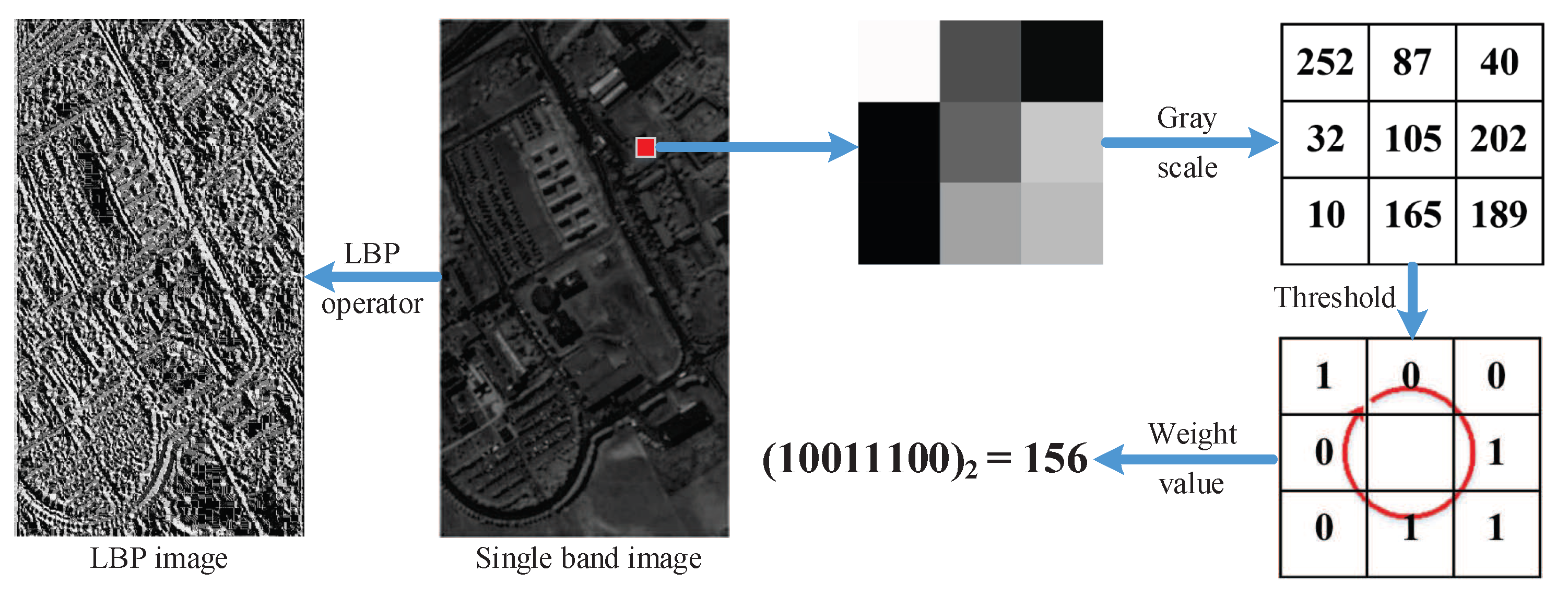
Local binary pattern is a discriminative and computationally local texture descriptor that has shown promising performance in classification. The original LBP operator represents the pixels of an image with binary numbers called LBP codes, which encode the local structure around each pixel, and then the codes are used for further analysis [29]. The procedure of it is shown in Figure 1, where the 10th band of PaviaU hyperspectral image is used to extract LBP features. As in Figure 1, for a given center pixel in a 3 × 3 window, the neighbor pixels are assigned with binary labels (“0” or “1”), depending on whether the gray value of center pixel is larger or not. An 8-digit binary number can be obtained by concatenating all these binary codes in a clockwise direction starting from the top-left one, and the derived binary numbers are referred to as LBP code.

According to the aforementioned analysis, spectral features and LBP features represent the information in HSI from different perspectives. Spectral features provide continuous spectral measurement across the entire electromagnetic spectrum, while LBP features present a better expression of detailed local spatial features, such as edges, corners, and knots. Thus, it is promising to apply LBP features as a supplement to spectral features that lack the consideration of spatial relations between pixels in HSI. However, both spectral features and LBP features are characterized by high dimensionality. A common approach to address the problem is to explore DR methods which will reduce the dimension of high-dimensional features largely without loss of information.

2.2. Graph Embedding

The GE framework is explored to unify many classical DR algorithms such as PCA, LDA, ISOMAP, LLE, LE, LPP and NPE. In GE, an intrinsic graph is constructed to characterize the statistical or geometrical properties that need to be preserved, and a penalty graph is explored to describe some properties which should be avoided. The intrinsic graph $G_I(X,W^w)$ and the penalty graph $G_p(X,W^b)$ are both undirected weighted graphs, where X is the vertex set of graph, $W^w\in {\Re }^{n\times n}$ and $W^b\in {\Re }^{n\times n}$ are the weight matrices of $G_I$ and $G_P$, respectively. $w_{ij}^w$ indicates the similarity between vertices $x_i$ and $x_j$ in $G_I$, while $w_{ij}^b$ measures the dissimilarity of vertices $x_i$ and $x_j$ in $G_P$. Under this framework, MFA has been proposed for dimensionality reduction of high-dimensioanl data. In MFA, $G_I$ connects each point with its neighbors from the same class to represent intraclass compactness, and $G_P$ connects the neighbor points which from different classes to represent the interclass separability. In low-dimensional embedding space, the intraclass compactness and interclass separability should be enhanced. Therefore, the optimal projection matrix V can be obtained with the following optimization problem:

$$J(V)=argmin\frac{{\sum }_{i,j}{∥V^T{x}_i-V^T{x}_j∥}^2{w}_{ij}^w}{{\sum }_{i,j}{∥V^T{x}_i-V^T{x}_j∥}^2{w}_{ij}^b}=argmin\frac{tr(V^{T}XL{X}^{T}V)}{tr(V^{T}X{L}^P{X}^{T}V)}$$

(1)

where $L=D^w-W^w$ is the Laplacian matrix of graph $G_I$, $W^w={[w_{ij}^w]}_{i,j=1}^n$, $D^w$ is a diagonal matrix, $D^w={[D_{ij}^w]}_{i,j=1}^n$, $D_{ii}^w={\displaystyle \sum _{j=1}^N}{w}_{ij}^w$, and $L^P=D^b-W^b$ is the Laplacian matrix of graph $G_P$, $W^b={[w_{ij}^b]}_{i,j=1}^n$, $D^b={[D_{ij}^b]}_{i,j=1}^n$, $D_{ii}^b={\displaystyle \sum _{j=1}^N}{w}_{ij}^b$.

3. Proposed Approach

Let us suppose that a hyperspectral data set $X=[x_1,x_2,x_3,\cdots ,x_N]\in {\Re }^{D\times N}$, where D is the number of bands and N indicates the number of pixels in HSI data. $X^S=\{x_i^s{\}}_{i=1}^N$ and $X^L=\{x_i^l{\}}_{i=1}^N$ denote the spectral features and LBP features of X, respectively. The class label of $x_i$ is indicated by $\ell (x_i)=\left\{1,2,\cdots ,c\right\}$, where c is the number of classes. The purpose of DR is to find a low-dimensional embedding space $Y=[y_1,y_2,y_3,\cdots ,y_N]\in {\Re }^{d\times N}$, where d$(d\ll D)$ is the embedding dimensionality of extracted features.

3.1. Motivation

Since different types of features represent HSI data from different perspectives, multiple feature fusion will bring benefits to enhance the discrimination capability for classification. The most common way to combine these features is to simply concatenate different types of features together, and then a classifier is employed to classify the stacked features. However, such stack-based methods have witnessed limited performance due to the simple strategy, and they may even perform worse than using a single feature in HSI data. The reasons for this phenomenon are summarized as follows:

• Simply stacking spatial and spectral features may yield redundant information, and it remains difficult to achieve an optimal combination for different kinds of features;
• The spatial information and spectral information is not equally represented by simply stacking;
• The stacked features greatly increase the dimensionality of spatial-spectral combined features, this will make HSI classification fairly challenging for the curse-of-dimensionality problem, especially when only limited training samples are available.

Many DR methods have been explored to reduce the dimension of stacked features. However, different types of features usually lie on different manifolds. Performing dimensionality reduction directly on the simply stacked features cannot reveal the manifold structure of different features in HSI. As a result, the discriminant information contained by different features is not effectively represented, which will restrict their discriminant capability for classification.

To overcome the shortcomings as discussed above, a new DR method called MFMDA is introduced in next section. By exploring the manifold structures of different features, it can effectively extract the spatial-spectral combined features and subsequently improve the classification performance of HSI.

3.2. MFMDA

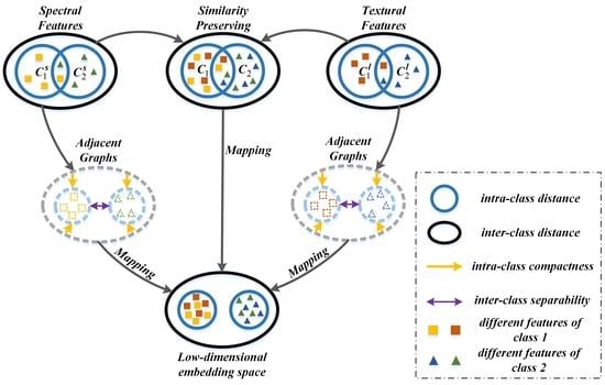
The goal of the proposed MFMDA method is to find an optimized projection matrix which can couple dimensionality reduction and data fusion of original features (from HSI data) and spatial features (LBP features generated from HSI) based on GE framework. MFMDA simultaneously learns a low-dimensional embedding space from original spectral features as well as LBP features for compacting the intramanifold samples while separating intermanifold samples, which will increase the margins between different manifolds. As a result, the obtained embedding features possess stronger discriminating ability that helps to subsequent classification. The flowchart of MFMDA is shown in Figure 2.

As illustrated in Figure 2, due to the fact that the similarity relationship between spectral features and LBP features from the same pixel should be preserved in the low-dimensional embedding space. Let us assume $A_S\in {\Re }^{\mathrm{D}\times \mathrm{d}}$ and $A_L\in {\Re }^{\mathrm{D}\times \mathrm{d}}$ are the corresponding projection matrices of spectral features and LBP features, respectively. $A_S$ and $A_L$ should be explored to minimize the distance between the two embedding features from the same pixel, and the objective function can be defined as follows:

$$J_1(A_S,A_L)=min{\displaystyle \sum _{i=1}^N}{∥A_S^T{x}_i^s-A_L^T{x}_i^l∥}^2$$

(2)

With some mathematical operations, Equation (2) can be reduced as:

$$\begin{array}{c}{J}_1(A_S,A_L)=min{{\displaystyle \sum _{i=1}^N}∥A_S^T{x}_i^s-A_L^T{x}_i^l∥}^2=tr({\displaystyle \sum _{i=1}^N}(A_S^T{x}_i^s-A_L^T{x}_i^l){(A_S^T{x}_i^s-A_L^T{x}_i^l)}^T)\hfill \\ =tr({\displaystyle \sum _{i=1}^N}(A_S^T{x}_i^s{(x_i^s)}^T{A}_S-A_L^T{x}_i^l{(x_i^s)}^T{A}_S-A_S^T{x}_i^s{(x_i^l)}^T{A}_L+A_L^T{x}_i^l{(x_i^l)}^T{A}_L))\hfill \\ =tr({\left[\begin{array}{cc}B& 0\\ 0& C\end{array}\right]}^T\left[\begin{array}{cc}{(X^S)}^T& 0\\ 0& {(X^L)}^T\end{array}\right]\left[\begin{array}{cc}{X}^S& 0\\ 0& X^L\end{array}\right]L_1\left[\begin{array}{cc}{(X^S)}^T& 0\\ 0& {(X^L)}^T\end{array}\right]\left[\begin{array}{cc}{X}^S& 0\\ 0& X^L\end{array}\right]\left[\begin{array}{cc}B& 0\\ 0& C\end{array}\right])\hfill \\ =tr(A^{T}E{L}_1{E}^{T}A)\hfill \end{array}$$

(3)

where $A_S$ and $A_L$ are respectively parameterized as $A_S=X^{S}B$ and $A_L=X^{L}C$, B and C are projection matrices that map spectral information and texture information in high-dimensional features to the low-dimensional embedded space, respectively. $A=\left[\begin{array}{cc}B& 0\\ 0& C\end{array}\right]$, $E=\left[\begin{array}{cc}{(X^S)}^T{X}^S& 0\\ 0& {(X^L)}^T{X}^L\end{array}\right]$, $L_1=\left[\begin{array}{cc}I& -I\\ -I& I\end{array}\right]$, I is the identity matrix in L.

From the view point of classification, in the low-dimensional embedding space, we expect that the samples are as close as possible if they belong to the same manifold, while samples are as far as possible if they are from different manifolds. To achieve this goal, we define the objective function as follows:

$$J_2(A_S,A_L)=min({\displaystyle \sum _{i=1}^N}{{\displaystyle \sum _{j=1}^N}∥A_S^T{x}_i^s-A_S^T{x}_j^s∥}^2{w}_{ij}^{w_s}+{\displaystyle \sum _{i=1}^N}{{\displaystyle \sum _{j=1}^N}∥A_L^T{x}_i^l-A_L^T{x}_j^l∥}^2{w}_{ij}^{w_l})$$

(4)

$$J_3(A_S,A_L)=max({\displaystyle \sum _{i=1}^N}{{\displaystyle \sum _{j=1}^N}∥A_S^T{x}_i^s-A_S^T{x}_j^s∥}^2{w}_{ij}^{b_s}+{\displaystyle \sum _{i=1}^N}{{\displaystyle \sum _{j=1}^N}∥A_L^T{x}_i^l-A_L^T{x}_j^l∥}^2{w}_{ij}^{b_l})$$

(5)

where $w_{ij}^{w_{\mathrm{s}}}$ and $w_{ij}^{b_{\mathrm{s}}}$ are the affinity weights to characterize the similarity between spectral features $x_i^s$ and $x_j^s$ of intrinsic graph $G_I^S$ as well as the dissimilarity between $x_i^s$ and $x_j^s$ of the penalty graph $G_P^S$, $w_{ij}^{w_l}$ and $w_{ij}^{b_l}$ are the affinity weights to characterize the similarity between LBP features $x_i^l$ and $x_j^l$ of the intrinsic graph $G_I^L$ and the dissimilarity between $x_i^l$ and $x_j^l$ of the penalty graph $G_P^L$, respectively.

In the intrinsic graph $G_I^S$ of spectral features, the vertices $x_i^s$ and $x_j^s$ are connected by an edge if $l(x_i)=l(x_j)$ and they are close to each other in terms of some distance. When it comes to the penalty graph $G_P^S$, the vertices $x_i^s$ and $x_j^s$ are connected by an edge if $l(x_i)\ne l(x_j)$ and $x_j^s$ belongs the $k_b$ nearest neighbors of $x_i^s$. The weights $w_{ij}^{w_{\mathrm{s}}}$ and $w_{ij}^{b_{\mathrm{s}}}$ in two spectral-based graphs are defined as:

$$w_{ij}^{w_{\mathrm{s}}}=\left\{\begin{array}{c}exp(-\frac{{∥x_i^s-x_j^s∥}^2}{2{(t_i^s)}^2}),x_i^s\in N_{{}_{s,w}}(x_j^s)or{x}_j^s\in N_{s,w}(x_i^s)\hfill \\ 0,otherwise\hfill \end{array}\right.$$

(6)

$$w_{ij}^{b_{\mathrm{s}}}=\left\{\begin{array}{c}exp(-\frac{{∥x_i^s-x_j^s∥}^2}{2{(t_i^s)}^2}),x_i^s\in N_{s,b}(x_j^s)or{x}_j^s\in N_{s,b}(x_i^s)\hfill \\ 0,otherwise\hfill \end{array}\right.$$

(7)

where $N_{s,w}(x_i^s)$ is the $n_w$-intramanifold neighbors of spectral feature $x_i^s$, $N_{s,b}(x_i^s)$ indicates the $n_b$-intermanifold neighbors of $x_i^s$, and $t_i^s=\frac{1}{n}{\displaystyle \sum _{j=1}^n}∥x_i^s-x_j^s∥$.

In the intrinsic graph $G_I^L$ of LBP features, an edge is added between the vertices $x_i^l$ and $x_j^l$ if $l(x_i)=l(x_j)$ and $x_j^l$ belongs the $k_w$ nearest neighbors of $x_i^l$; in the penalty graph $G_P^L$, an edge is connected by $x_i^l$ and $x_j^l$ if $l(x_i)\ne l(x_j)$ and $x_j^l$ belongs the $k_b$ nearest neighbors of $x_i^l$. The weights $w_{ij}^{w_{\mathrm{l}}}$ and $w_{ij}^{b_{\mathrm{l}}}$ in two LBP-based graphs can be set as:

$$w_{ij}^{w_l}=\left\{\begin{array}{c}exp(-\frac{{∥x_i^l-x_j^l∥}^2}{2{(t_i^l)}^2}),x_i^l\in N_{l,w}(x_j^l)or{x}_j^l\in N_{l,w}(x_i^l)\hfill \\ 0,otherwise\hfill \end{array}\right.$$

(8)

$$w_{ij}^{b_l}=\left\{\begin{array}{c}exp(-\frac{{∥x_i^l-x_j^l∥}^2}{2{(t_i^l)}^2}),x_i^l\in N_{l,b}(x_j^l)or{x}_j^l\in N_{l,b}(x_i^l)\hfill \\ 0,otherwise\hfill \end{array}\right.$$

(9)

where $N_{l,w}(x_i^l)$ is the $n_w$-intramanifold neighbors of spectral feature $x_i^l$, $N_{l,b}(x_i^l)$ indicates the $n_b$-intermanifold neighbors of $x_i^l$, and $t_i^l=\frac{1}{n}{\displaystyle \sum _{j=1}^n}∥x_i^l-x_j^l∥$.

The objective function of $J_2(A_S,A_L)$ in Equation (4) is to minimize the intramanifold distance to ensuring the samples from the same manifold should be as close as possible, and the objective function of $J_3(A_S,A_L)$ in Equation (5) is to maximize the intermanifold distance for enlarging the manifold margins in the low-dimensional embedding space.

With some mathematical operations, Equations (4) and (5) can be reduced as:

$$\begin{array}{c}{\displaystyle \sum _{i=1}^N}{{\displaystyle \sum _{j=1}^N}∥A_S^T{x}_i^s-A_S^T{x}_j^s∥}^2{w}_{ij}^{w_s}+{\displaystyle \sum _{i=1}^N}{{\displaystyle \sum _{j=1}^N}∥A_L^T{x}_i^l-A_L^T{x}_j^l∥}^2{w}_{ij}^{w_l}\hfill \\ =tr({\displaystyle \sum _{i=1}^N}{\displaystyle \sum _{j=1}^N}(A_S^T{x}_i^s{w}_{ij}^{w_s}{(x_i^s)}^T{A}_S-2A_S^T{x}_i^s{w}_{ij}^{w_s}{(x_j^s)}^T{A}_S+A_S^T{x}_j^s{w}_{ij}^{w_s}{(x_j^s)}^T{A}_S)\hfill \\ +{\displaystyle \sum _{i=1}^N}{\displaystyle \sum _{j=1}^N}(A_L^T{x}_i^l{w}_{ij}^{w_l}{(x_i^l)}^T{A}_L-2A_L^T{x}_i^l{w}_{ij}^{w_l}{(x_j^l)}^T{A}_L+A_L^T{x}_i^l{w}_{ij}^{w_l}{(x_i^l)}^T{A}_L))\hfill \\ =tr({\left[\begin{array}{cc}B& 0\\ 0& C\end{array}\right]}^T\left[\begin{array}{cc}{(X^S)}^T& 0\\ 0& {(X^L)}^T\end{array}\right]\left[\begin{array}{cc}{X}^S& 0\\ 0& X^L\end{array}\right]L_2\left[\begin{array}{cc}{(X^S)}^T& 0\\ 0& {(X^L)}^T\end{array}\right]\left[\begin{array}{cc}{X}^S& 0\\ 0& X^L\end{array}\right]\left[\begin{array}{cc}B& 0\\ 0& C\end{array}\right])\hfill \\ =tr(A^{T}E{L}_2{E}^{T}A)\hfill \end{array}$$

(10)

$$\begin{array}{c}{\displaystyle \sum _{i=1}^N}{{\displaystyle \sum _{j=1}^N}∥A_S^T{x}_i^s-A_S^T{x}_j^s∥}^2{w}_{ij}^{b_s}+{\displaystyle \sum _{i=1}^N}{{\displaystyle \sum _{j=1}^N}∥A_L^T{x}_i^l-A_L^T{x}_j^l∥}^2{w}_{ij}^{b_l}\hfill \\ =tr({\displaystyle \sum _{i=1}^N}{\displaystyle \sum _{j=1}^N}(A_S^T{x}_i^s{w}_{ij}^{b_s}{(x_i^s)}^T{A}_S-2A_S^T{x}_i^s{w}_{ij}^{b_s}{(x_j^s)}^T{A}_S+A_S^T{x}_j^s{w}_{ij}^{b_s}{(x_j^s)}^T{A}_S)\hfill \\ +{\displaystyle \sum _{i=1}^N}{\displaystyle \sum _{j=1}^N}(A_L^T{x}_i^l{w}_{ij}^{b_l}{(x_i^l)}^T{A}_L-2A_L^T{x}_i^l{w}_{ij}^{b_l}{(x_j^l)}^T{A}_L+A_L^T{x}_i^l{w}_{ij}^{b_l}{(x_i^l)}^T{A}_L))\hfill \\ =tr({\left[\begin{array}{cc}B& 0\\ 0& C\end{array}\right]}^T\left[\begin{array}{cc}{(X^S)}^T& 0\\ 0& {(X^L)}^T\end{array}\right]\left[\begin{array}{cc}{X}^S& 0\\ 0& X^L\end{array}\right]L_3\left[\begin{array}{cc}{(X^S)}^T& 0\\ 0& {(X^L)}^T\end{array}\right]\left[\begin{array}{cc}{X}^S& 0\\ 0& X^L\end{array}\right]\left[\begin{array}{cc}B& 0\\ 0& C\end{array}\right])\hfill \\ =tr(A^{T}E{L}_3{E}^{T}A)\hfill \end{array}$$

(11)

where $L_2=\left[\begin{array}{cc}2(D^{w_s}-W^{w_s})& 0\\ 0& 2(D^{w_l}-W^{w_l})\end{array}\right]$, $W^{w_s}={\left[w_{ij}^{w_s}\right]}_{i,j=1}^N$, $W^{w_l}={\left[w_{ij}^{w_l}\right]}_{i,j=1}^N$, $D^{w_s}=diag([{\displaystyle \sum _{j=1}^N}{w}_{ij}^{w_s}{]}_{i=1}^N)$, $D^{w_l}=diag([{\displaystyle \sum _{j=1}^N}{w}_{ij}^{w_l}{]}_{i=1}^N)$; $L_3=\left[\begin{array}{cc}2(D^{b_s}-W^{b_s})& 0\\ 0& 2(D^{b_l}-W^{b_l})\end{array}\right]$, $W^{b_s}={\left[w_{ij}^{b_s}\right]}_{i,j=1}^N$, $W^{b_l}={\left[w_{ij}^{b_l}\right]}_{i,j=1}^N$, $D^{b_s}=diag([{\displaystyle \sum _{j=1}^N}{w}_{ij}^{b_s}{]}_{i=1}^N)$, $D^{b_l}=diag([{\displaystyle \sum _{j=1}^N}{w}_{ij}^{b_l}{]}_{i=1}^N)$.

As discussed, the MFMDA method not only preserves the similarity relationship between spectral features and LBP features but also possesses strong discriminating ability in the low-dimensional embedding space. Therefore, a reasonable criterion for choosing a good projection matrix is to optimize the following objective functions:

$$\left\{\begin{array}{c}mintr(A^{T}E{L}_1{E}^{T}A)\\ mintr(A^{T}E{L}_2{E}^{T}A)\\ maxtr(A^{T}E{L}_3{E}^{T}A)\end{array}\right.$$

(12)

The multi-objective function optimization problem in Equation (12) can be equivalent to:

$$\begin{array}{c}J(A_S,A_L)=min\{tr(A^{T}E{L}_1{E}^{T}A)+\alpha (tr(A^{T}E{L}_2{E}^{T}A))-\beta (tr(A^{T}E{L}_3{E}^{T}A)\}\hfill \\ =min\left\{tr(A^{T}EL{E}^{T}A)\right\}\hfill \end{array}$$

(13)

where $\alpha$, $\beta$ > 0 are two tradeoff parameters which can adjust intramanifold compactness and intermanifold separability, $L=L_1+\alpha L_2-\beta L_3$.

A constraint $A^{T}E{E}^{T}A=I$ is imposed to remove an arbitrary scaling factor in the projection, and the objective function can be recast as follows:

$$\left\{\begin{array}{c}min(tr(A^{T}EL{E}^{T}A))\\ s.t.A^{T}E{E}^{T}A=I\end{array}\right.$$

(14)

With the method of Lagrangian multiplier, the optimization solution is formulated as

$$\frac{\partial }{\partial A}tr(A^{T}EL{E}^{T}A-\lambda (A^{T}E{E}^{T}A-I))=0$$

(15)

where $\lambda$ is the Lagrangian multiplier. Then the optimization problem is transformed to solve a generalized eigenvalue problem, i.e.,

$$EL{E}^{T}A=\lambda E{E}^{T}A$$

(16)

where the optimal projection matrix $A=[a_1,a_2,\cdots ,a_d]$ is composed of d minimum eigenvalues of Equation (16) corresponding eigenvectors. Then the low-dimensional feature is given by:

$$\begin{array}{cc}\hfill y_i& =\left[\begin{array}{c}{y}_i^s\\ y_i^l\end{array}\right]=\left[\begin{array}{c}{A}_S^T{x}_i^s\\ A_L^T{x}_i^l\end{array}\right]=\left[\begin{array}{c}{(X^{S}B)}^T{x}_i^s\\ {(X^{L}C)}^T{x}_i^l\end{array}\right]=\left[\begin{array}{cc}{(X^{S}B)}^T& 0\\ 0& {(X^{L}C)}^T\end{array}\right]\left[\begin{array}{c}{x}_i^s\\ x_i^l\end{array}\right]\hfill \\ & ={\left[\begin{array}{cc}B& 0\\ 0& C\end{array}\right]}^T\left[\begin{array}{cc}{(X^S)}^T& 0\\ 0& {(X^L)}^T\end{array}\right]\left[\begin{array}{c}{x}_i^s\\ x_i^l\end{array}\right]\hfill \end{array}$$

(17)

The proposed MFMDA algorithm is summarized in Algorithm 1.

Algorithm 1 MFMDA.

Input:  data set $X=[x_1,x_2,x_3,\cdots ,x_N]\in {\Re }^{D\times N}$, corresponding class labels $\ell (x_i)=\left\{1,2,\cdots ,c\right\}$, the number of intraclass neighbor points $n_w$ and the number of interclass neighbor points $n_b$, balance parameter $\alpha$ and $\beta$.   1: Get LBP features generated from the data set, $X^S=\{x_i^s{\}}_{i=1}^N\in {\Re }^{D\times N}$ and $X^L=\{x_i^l{\}}_{i=1}^N\in {\Re }^{D\times N}$ denote the spectral and LBP features.   2: Find the $n_w$ intraclass neighbor points and $n_b$ interclass neighbor points of spectral features and LBP features, respectively.   3: Calculate the edge weights of the intrinsic and penalty graphs by Equations (6)–(9).   4: Compute the $D^{w_s}$, $D^{w_l}$, $D^{b_s}$ and $D^{b_l}$ by $D^{w_s}=diag([{\displaystyle \sum _{j=1}^N}{w}_{ij}^{w_s}{]}_{i=1}^N)$, $D^{w_l}=diag([{\displaystyle \sum _{j=1}^N}{w}_{ij}^{w_l}{]}_{i=1}^N)$, $D^{b_s}=diag([{\displaystyle \sum _{j=1}^N}{w}_{ij}^{b_s}{]}_{i=1}^N)$ and $D^{b_l}=diag([{\displaystyle \sum _{j=1}^N}{w}_{ij}^{b_l}{]}_{i=1}^N)$, respectively.   5: Obtain the Lagrangian matrix which contain manifold structure through $L=L_1+\alpha L_2-\beta L_3$.    6: Calculate matrix E by $E=\left[\begin{array}{cc}{(X^S)}^T{X}^S& 0\\ 0& {(X^L)}^T{X}^L\end{array}\right]$.   7: Construct the matrix $A=[a_1,a_2,\cdots ,a_d]$ according to Equation (16).   8: Obtain the projection matrix of spectral and LBP features by $A=\left[\begin{array}{cc}B& 0\\ 0& C\end{array}\right]$, $A_S=X^{S}B$ and $A_L=X^{L}C$.   9: Achieve the low-dimensional features Y through Equation (17). Output:  $Y=[y_1,y_2,y_3,\cdots ,y_N]\in {\Re }^{d\times N},d\ll D$; Projection matrix of spectral and LBP features: $A_S=X^{S}B$ and $A_L=X^{L}C$.

4. Experimental Results and Discussion

In this section, experiments are conducted on three real HSI data sets to evaluate the effectiveness of the proposed MFMDA method.

4.1. Experiment Data Set

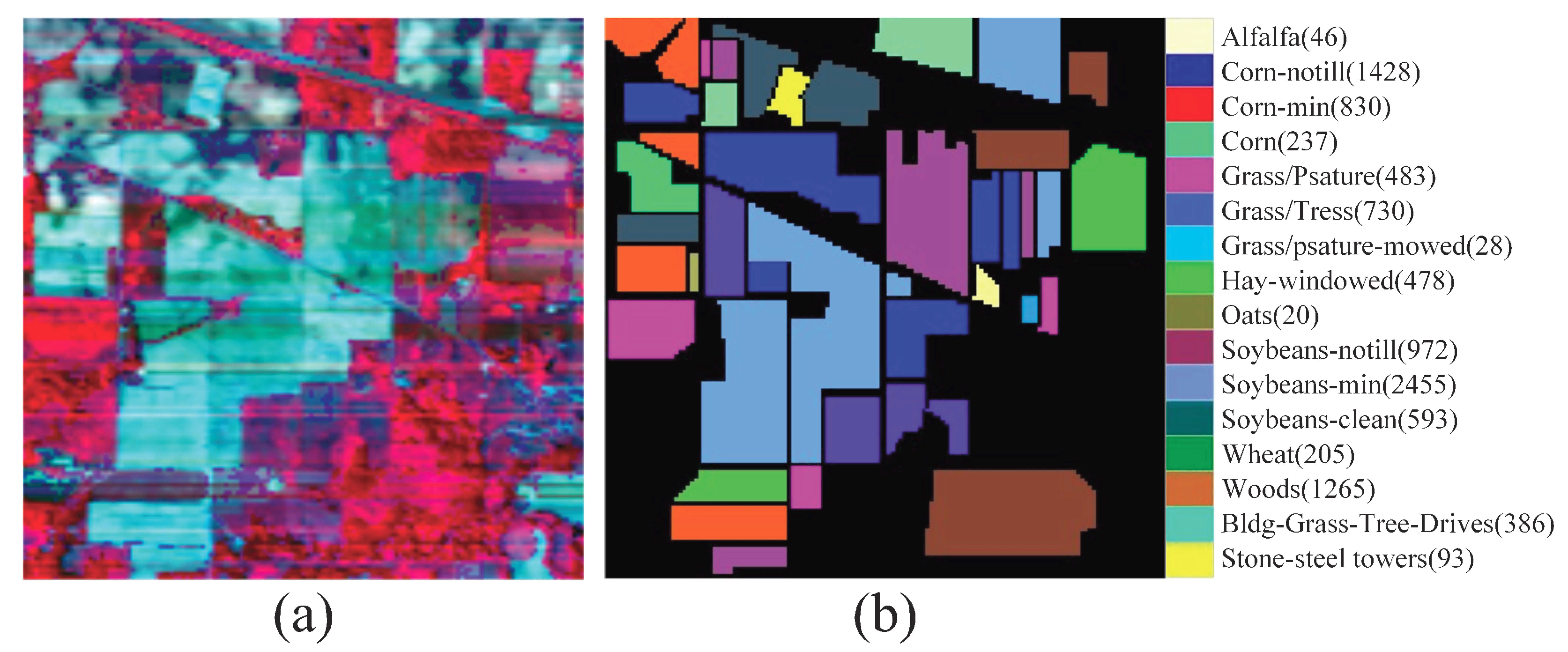
Indian Pines data set: This HSI data set was collected by NASA using the Airborne Visible/Infrared Imaging Spectrometer (AVIRIS) sensor in Northwest Indiana. After removing water absorption bands, the remaining 200 bands were used in the experiments. The size of this image is 145 × 145 pixels with a spatial resolution of 20 m, and it contains sixteen land cover types such as Wheat, Woods and Oats. This scene in false color and its corresponding ground truth are shown in Figure 3, and the values in brackets indicate the sample size of each class.

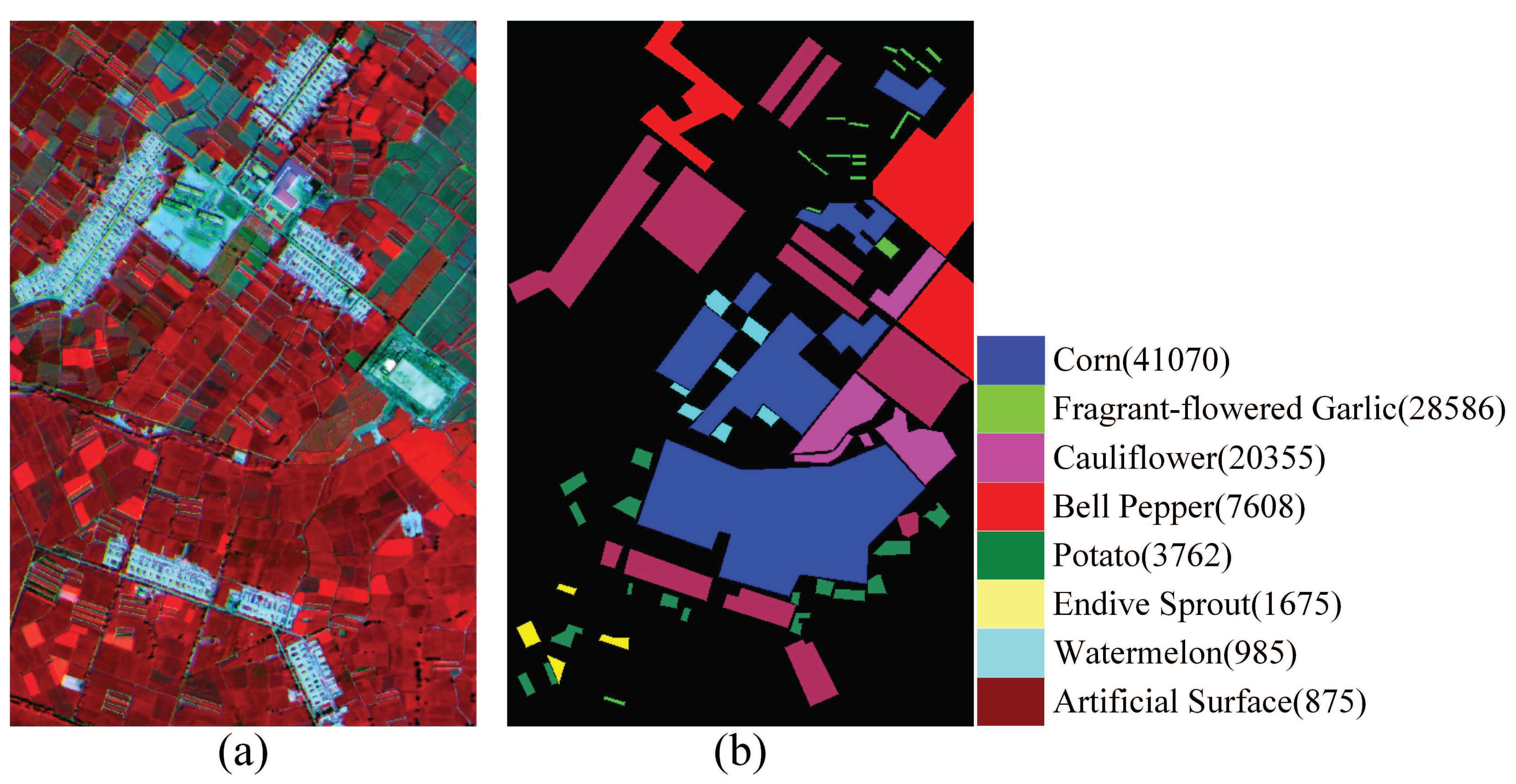
Heihe data set [55,56]: This data set is provided by Heihe Plan Science Data Center which is sponsored by the integrated research on the eco-hydrological process of the Heihe River Basin of the National Natural Science Foundation of China, and it was captured by Compact Airborne Spectrographic Imager (CASI)/Shortwave Infrared Airborne Spectrogrpahic Imager (SASI) in Zhangye basin which is located in the middle reaches of Heihe watershed, Gansu Province, China. The data possesses a spatial size of 684 × 453 pixels, and it has a geometric resolution of 2.4 m. Exactly 135 bands remained after removal of 14 bands which have noise and atmospheric effects. The data contains 9 different kinds of land covers. The scene in false color and its ground-truth map are shown in Figure 4.

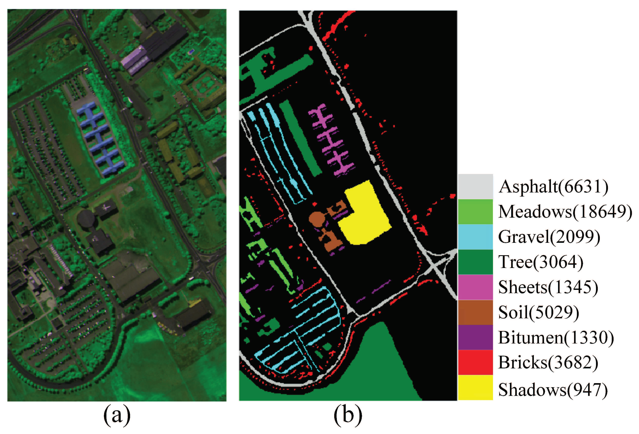
PaviaU data set: This data set is a scene of the PaviaU collected by the reflective optics system imaging spectrometer (ROSIS) sensor. It consists of 610 × 340 pixels and the spatial resolution is 1.3 m. 103 spectral bands remained after the removal of some channels as a result of dense water vapor and atmospheric effects. There are nine classes of ground objects are considered in the data set such as trees, soil and meadows. This HSI in false color and its corresponding ground truth are shown in Figure 5.

4.2. Experimental Setup

In each experiment, the HSI data set was randomly divided into training and test sets. For the classes that are very small, i.e., Alfalfa, Grass/pasture-mowed, and Oats in Indian Pines data set, the number of training samples was set to 10 per class. The training samples are used to learn a low-dimensional embedding space, then all test samples are mapped into the embedding space for extracting low-dimensional features. After that, support vector machine (SVM) with the radial basis function (RBF) kernel were used to classify test samples, and the library for SVM (LibSVM) Toolbox was employed to implement SVM [57]. The parameters for SVM were optimized by a grid search. The classification accuracy for each class, overall classification accuracies (OAs), average classification accuracies (AAs), and kappa coefficient (k) are used to evaluate the classification performance of different DR methods. To robustly evaluate the performance of different methods under different conditions, we repeated the experiments 10 times in each condition, and presented the results in the form of mean with standard deviation (STD).

The proposed MFMDA algorithm was compared with some state-of-art DR algorithms including Baseline, PCA [39], LDA [40], NPE [46], LPP [44], MFA [48] and LGSFA [51], where Baseline represents that test samples are classified directly by a classifier without dimensionality reduction. To verify the effectiveness of MFMDA, the above DR algorithms were applied to spectral features, LBP features and stacked features, respectively. Notice that LBP features are obtained by the “uniform LBP” pattern, and the ratio of neighborhood radius and the number of sampling points are set to 1 and 8, respectively [58]. The stacked features refer to stack original spectral features and LBP features after applying normalization.

For all methods, the parameters are optimized by using cross validation to achieve good results. The numbers of neighbors for NPE and LPP is set to 9. For MFA and LGSFA, the numbers of intraclass and interclass neighbors are chosen as 9 and 180, respectively. All experiments were performed on a personal computer with i7-7800X central processing unit, 32-G memory, and 64-bit Windows 10 using MATLAB 2014b.

4.3. Dimension Selection

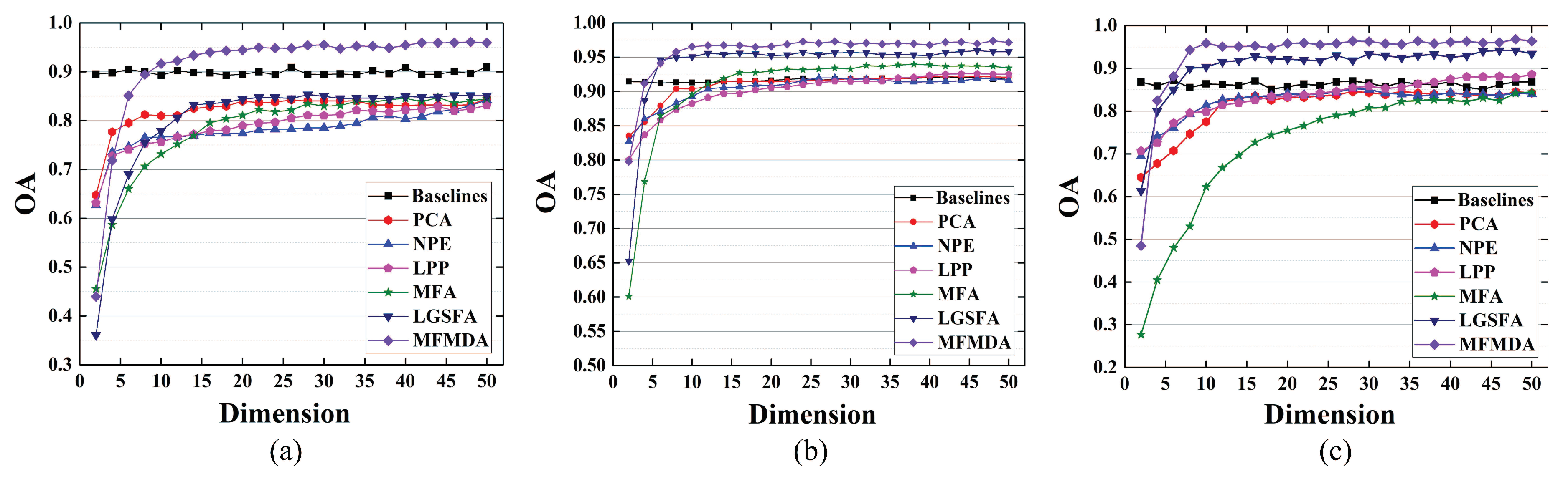
To analyze the influence of different embedding dimensions on each DR algorithm, 40 samples were randomly selected from the stacked features of each class in three HSI data sets for training, and the remaining samples were tested. Figure 6 shows the overall classification accuracy under different embedding sizes.

As shown in Figure 6, with the increase of embedding dimension, the OAs of all methods are gradually improved. The reason for this is that the more discriminant information can be contained with the increase of embedding features, which is helpful for classification. However, when the dimension has been increased to a certain extent, the low-dimensional embedding space contains enough information for classification, and then the increase of embedding dimension has little effect on the improvement of classification performance. Meanwhile, MFMDA achieves better classification results than other methods, because the MFMDA can better characterize the intrinsic manifold structure of HSI and obtain more effective low-dimensional discriminant features. To achieve better classification performance for each algorithm, the embedding dimensions of all methods are set to 40. When it comes to LDA, the embedding dimension is set to $c-1$, and c is the class number of the data set.

4.4. Experiments on the Indian Pines Data Set

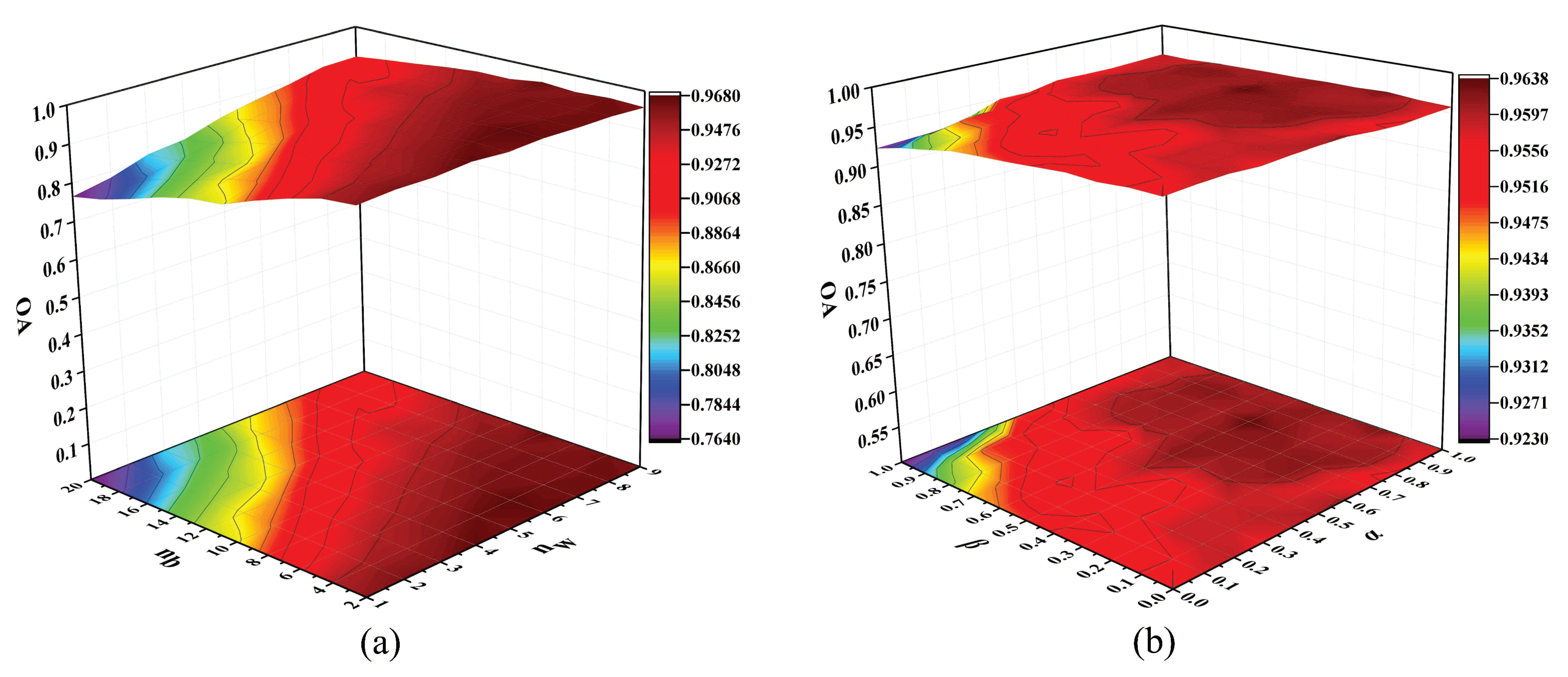
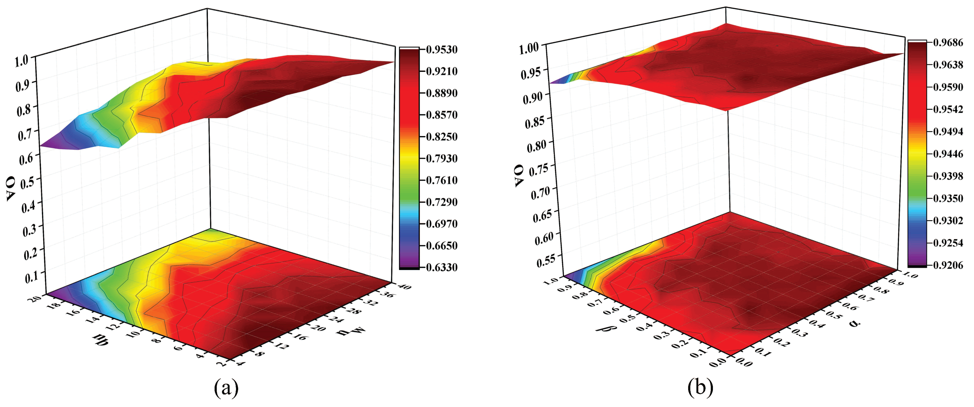
In this section, the experiments were conducted on the Indian Pines data set to evaluate the effectiveness of the proposed algorithm. The proposed MFMDA method has different parameters, and we conducted experiments to analysis the sensitivity of parameters. In the experiments, 40 samples per class were randomly selected for training, and the remaining ones for testing. The SVM classifier is used for classification. To investigate the classification influence on intraclass and interclass neighbors, parameters $n_w$ and $n_b$ are tuned with a set of {1,2,3,⋯,9} and a set of {2,4,6,⋯,20}, respectively. Figure 7a shows the OAs with different values of $n_w$ and $n_b$. When it comes to tradeoff parameters, parameters $\alpha$ and $\beta$ are all tuned with the set of {0,0.1,0.2,⋯,1}. The OAs with different values of $\alpha$ and $\beta$ are displayed in Figure 7b.

As can be seen in Figure 7a, with the increase of $n_w$, the classification accuracy improves and then tends to be stable, for the reason is that a large number of intraclass neighbors are conducive to reveal the intrinsic structure of HSI data. When the value of $n_w$ is lower than 7, the OAs maintain a stable value with an increase of $n_b$, but the OAs significantly decline when the value of $n_b$ exceeded 10. The reason is that too large values of $n_b$ will cause the phenomenon of over-learning in the margins between interclass samples. In Figure 7b, the classification performance improves with the increase of parameter $\alpha$ and then slightly fluctuates. While the proposed method can achieve good results at a wide range. However, when $\beta$ has a very large value, the effect of the intraclass separability will be limited. Thus, parameters $\alpha$ and $\beta$ can balance the contribution between intraclass compactness and interclass separability. According to this figure, we set the parameters $n_w$ and $n_b$ to 6 and 4, $\alpha$ and $\beta$ to 0.8 and 0.5 for achieving a satisfactory performance.

To analyze the classification performance of each algorithm under different numbers of training samples, $n_i$ ($n_i$ = 5, 10, 20, 30, 40) samples were randomly selected from each class for training, and the remaining data were used as test samples.

Table 1. Classification results using different methods with different classifiers for the Indian Pines data set. [Overall Accuracy ± Std (%)].

	Algorithm	${\mathit{n}}_{\mathit{i}}$ = 5	${\mathit{n}}_{\mathit{i}}$ = 10	${\mathit{n}}_{\mathit{i}}$ = 20	${\mathit{n}}_{\mathit{i}}$ = 30	${\mathit{n}}_{\mathit{i}}$ = 40
	Baseline	42.21 ± 4.63	53.72 ± 3.97	64.05 ± 2.03	69.72 ± 1.25	69.78 ± 1.58
	PCA	42.00 ± 5.56	53.35 ± 4.70	64.04 ± 1.73	68.07 ± 1.05	68.72 ± 1.59
Spectral	LDA	40.27 ± 4.46	40.29 ± 1.76	52.93 ± 1.44	61.00 ± 0.84	63.51 ± 1.23
Features	NPE	34.25 ± 6.33	48.49 ± 3.36	60.61 ± 1.45	65.82 ± 1.76	67.22 ± 1.63
	LPP	35.40 ± 5.40	47.41 ± 2.77	60.14 ± 2.37	66.64 ± 1.82	69.10 ± 1.51
	MFA	42.98 ± 4.78	49.66 ± 1.71	60.38 ± 2.59	64.09 ± 1.87	66.16 ± 0.89
	LGSFA	41.26 ± 5.35	49.57 ± 3.00	60.95 ± 1.91	66.40 ± 0.65	68.81 ± 1.36
	Baseline	68.12 ± 5.00	79.07 ± 2.97	87.58 ± 1.66	90.36 ± 2.82	93.54 ± 1.53
	PCA	65.72 ± 6.98	75.50 ± 4.09	83.89 ± 2.15	86.37 ± 3.40	89.80 ± 1.35
LBP	LDA	71.30 ± 3.75	79.69 ± 3.24	87.62 ± 1.78	91.02 ± 2.04	93.63 ± 1.25
Features	NPE	66.71 ± 4.61	75.06 ± 4.32	84.60 ± 1.95	86.55 ± 1.89	89.87 ± 1.24
	LPP	65.88 ± 2.80	75.73 ± 4.51	85.17 ± 1.97	87.71 ± 1.55	89.77 ± 0.85
	MFA	65.60 ± 7.20	75.69 ± 4.70	84.68 ± 1.63	85.73 ± 2.55	90.34 ± 1.24
	LGSFA	65.59 ± 2.11	74.90 ± 5.18	84.92 ± 1.70	87.86 ± 1.67	91.34 ± 1.34
	Baseline	56.36 ± 5.70	73.25 ± 2.15	82.74 ± 2.33	89.46 ± 1.49	90.83 ± 1.62
	PCA	54.22 ± 5.04	68.83 ± 2.83	76.39 ± 1.66	81.34 ± 1.30	83.71 ± 1.25
Stacked	LDA	70.06 ± 4.65	84.37 ± 2.34	89.58 ± 2.52	92.93 ± 0.59	94.24 ± 1.26
Features	NPE	56.02 ± 6.91	66.73 ± 3.68	74.37 ± 2.51	76.28 ± 1.71	78.62 ± 0.91
	LPP	58.08 ± 4.73	70.81 ± 2.49	74.43 ± 2.54	78.59 ± 1.36	79.30 ± 0.73
	MFA	53.94 ± 2.49	69.44 ± 2.47	77.15 ± 2.12	80.57 ± 2.70	82.94 ± 1.83
	LGSFA	63.83 ± 5.17	73.35 ± 1.03	79.10 ± 0.37	83.15 ± 1.77	84.57 ± 0.57
MFMDA		74.01 ± 5.72	85.74 ± 2.42	91.79 ± 2.39	94.61 ± 1.15	96.19 ± 0.89

Notes: The bold numbers represent the maximum OA of the column.

shows the average OAs with STD for different DR methods with different numbers of training samples.

According to Table 1, with the increase in the sample size of training set, the OAs of all methods continuously raise, for the reason is that a large training set contains more available information to learn discriminant features for classification. Furthermore, the classification results of each algorithm on LBP features are superior to that of spectral features, this is because LBP features are spatial-based features which bring benefits to classification. However, the classification performance of simply stacked features is even worse than LBP features, this may be due to the fact that spatial features and spectral features are not equally represented by simply stacking. While the proposed MFMDA algorithm produces a better classification effect than other methods in all conditions, especially when there are only a small number of labeled samples. The reason for this is that the proposed algorithm not only guarantees the similarity for spectral features and LBP features of the same pixel in the low-dimensional embedding space, but also discovers the manifold structure in the hyperspectral data by constructing intrinsic graphs and penalty graphs, and then extracts the spatial-spectral combined discriminant features to achieve the compactness for intraclass data and the separability for interclass data.

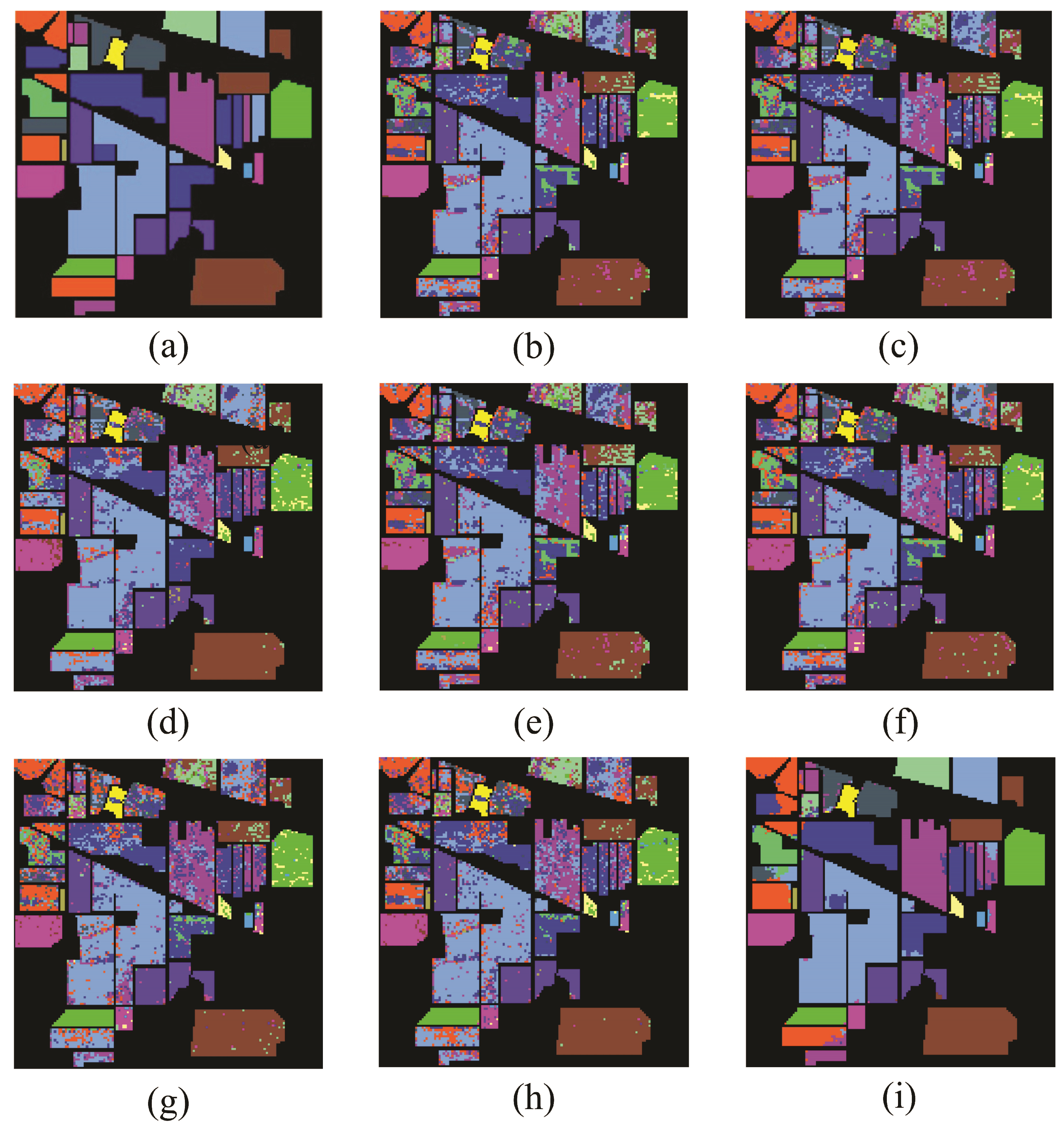
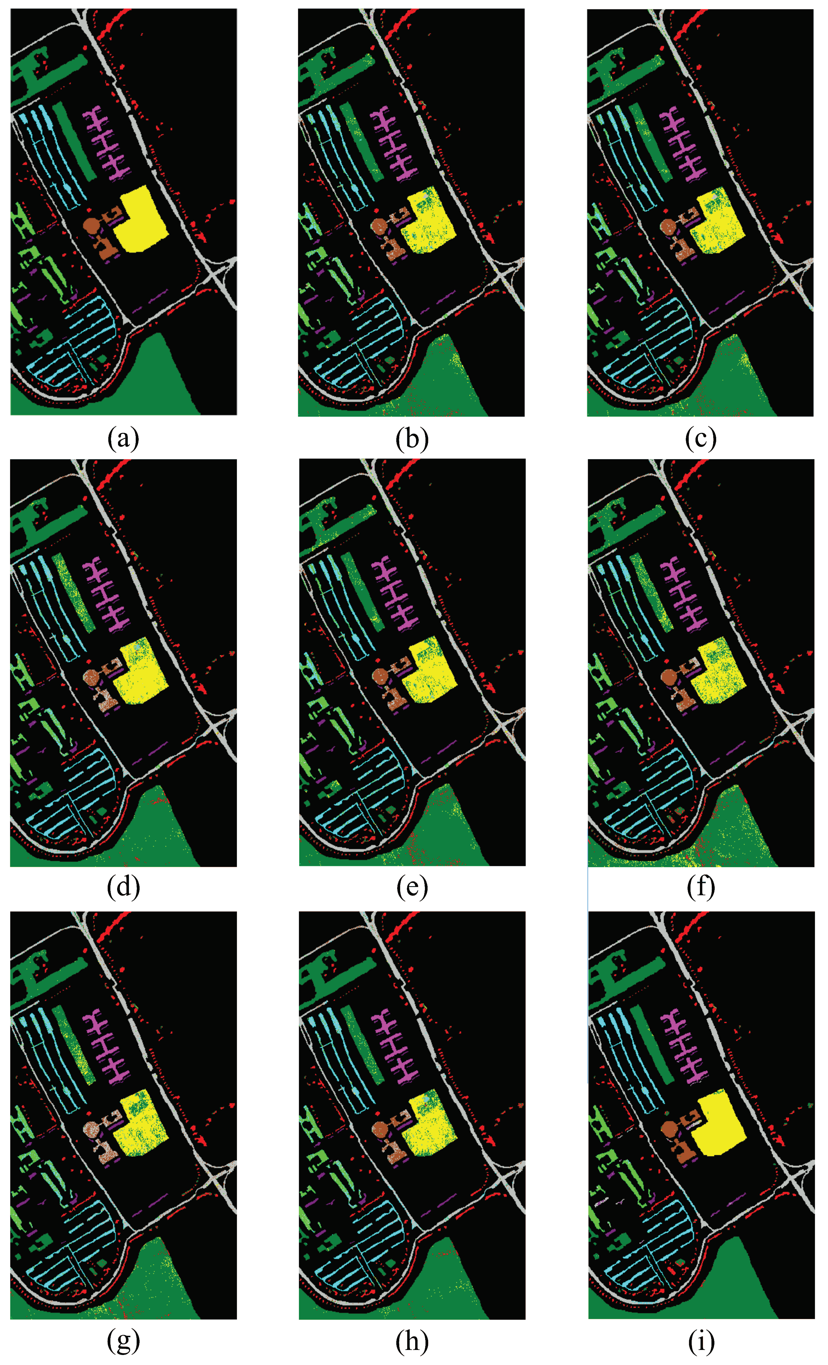
To explore the classification performance of MFMDA on each class, 3% samples per class were randomly selected for training, and remaining samples were used for testing. We can see from Table 1, the experimental results of DR methods on LBP features are better than spectral features and stacked features, and thus LBP features were chosen for comparison in the following experiments.

Table 2. Classification results of each class samples via different DR methods in Indian Pines data set (%).

Class	Samples		DR with SVM Classifier
	Train	Test	Baseline	PCA	LDA	NPE	LPP	MFA	LGSFA	MFMDA
1	10	36	99.72	99.17	98.89	99.44	99.72	99.44	99.44	96.67
2	43	1385	93.91	92.94	93.86	92.25	93.23	94.09	93.10	93.33
3	25	805	94.31	92.42	93.74	92.01	91.69	91.66	92.46	92.57
4	10	227	95.37	94.85	94.98	92.73	93.66	94.98	94.23	93.17
5	14	469	84.54	82.41	83.22	83.71	84.86	82.90	84.61	90.00
6	22	708	93.29	92.97	92.19	92.13	91.44	92.20	91.91	98.18
7	10	18	100	100	100	100	100	100	100	98.89
8	14	464	98.53	98.38	98.41	97.91	98.38	97.80	97.95	99.74
9	10	10	100	100	100	100	100	100	99.00	100
10	29	943	89.72	88.23	90.38	88.29	87.41	89.00	88.09	91.56
11	74	2381	95.46	94.93	95.72	94.51	94.49	95.08	95.09	97.96
12	18	575	87.84	83.34	88.52	85.63	85.76	86.73	87.06	92.28
13	10	195	96.36	95.74	95.85	94.67	95.49	94.72	95.85	98.15
14	38	1227	96.85	96.27	97.42	95.98	96.09	96.10	95.75	99.62
15	12	374	87.86	89.12	84.47	87.54	88.34	86.47	87.99	96.52
16	10	83	95.78	96.27	92.89	96.39	96.39	96.27	95.42	99.52
OA			93.57	92.57	93.43	92.29	92.43	92.78	92.72	95.71
AA			94.35	93.56	93.78	93.33	93.56	93.59	93.62	96.14
Kappa			0.93	0.92	0.92	0.91	0.91	0.92	0.92	0.95

Notes: The bold numbers represent the maximum OA of the row.

lists the classification accuracy of each class, OAs, AAs, and Kappa coefficients of different methods, and Figure 8 shows the corresponding classification maps.

As illustrated in Table 2, the MFMDA algorithm achieved good classification results in most classes, especially for the areas labeled as Wheat, Grass/Trees, Soybeans-min and Woods. By observing Figure 8, the classification map of MFMDA algorithm produced more homogenous regions than other methods.

The above results show that the proposed method compacts spectral features and LBP features from the same class and separates the features belong to different classes in low-dimensional embedding space, it can make better use of the manifold structure hidden in hyperspectral data.

4.5. Experiments on the Heihe Data Set

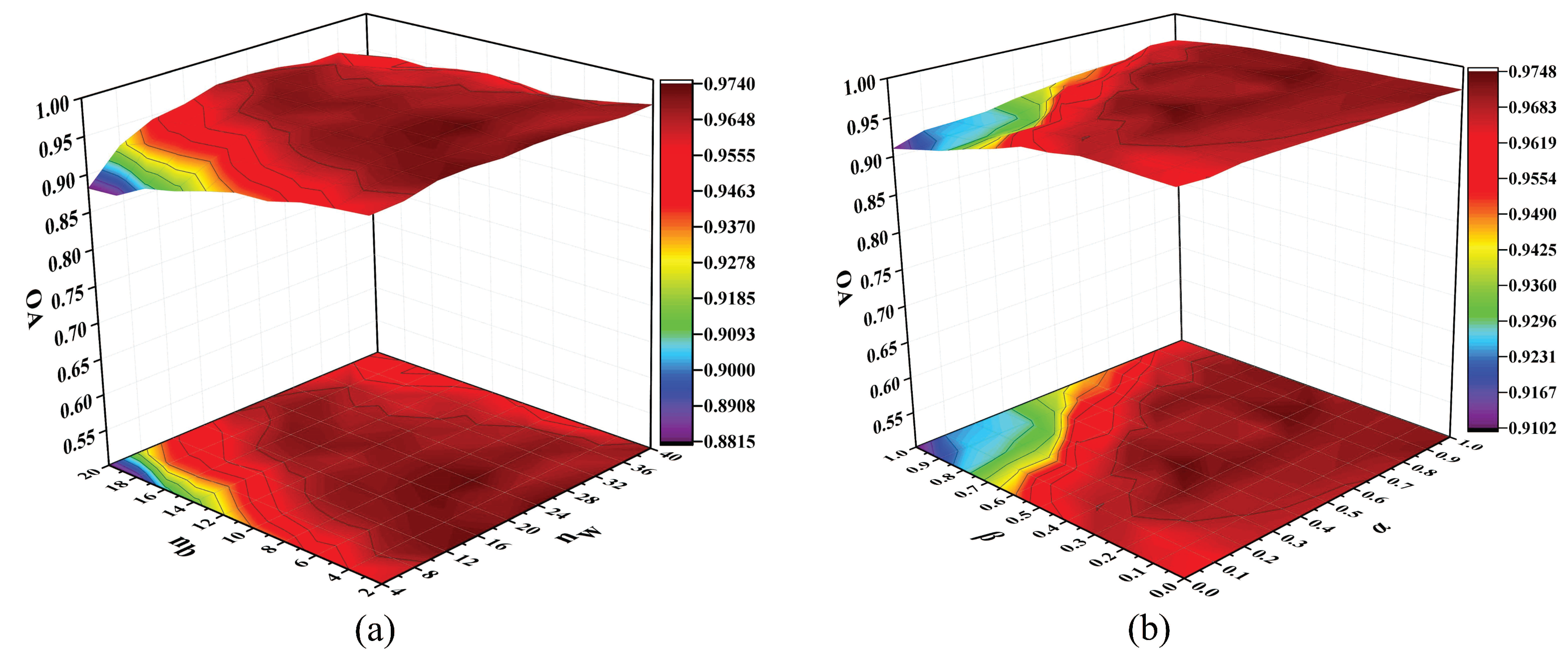
In this section, the Heihe hyperspectral image was used to further evaluate the classification performance of the proposed algorithm. In the parameter sensitivity experiments, we randomly selected 40 samples from each class for training and the rest for testing. At first, we analyze the influence of different parameters on MFMDA algorithm, and the OAs with different values of parameters are displayed in Figure 9.

As in Figure 9a, the OA increases and then declines with the increase of n${}_w$, it is because a small value of n${}_w$ cannot get enough information to represent the intraclass structure, and a large value of n${}_w$ will lead to overfitting. At the same time, an appropriate size of interclass neighbor points can prevent overfitting and effectively obtain discriminant information of HSI data. In Figure 9b, it can be observed that the OAs increase and then maintain slight fluctuation with the increase of $\alpha$, and a too small value of $\beta$ will lead to unsatisfactory classification performance. This indicates that the suitable $\alpha$ and $\beta$ can balance the intramanifold and intermanifold relations of spectral features and textual features. Based on the above analysis, we set the parameters $n_w$ and $n_b$ to 24 and 6, $\alpha$ and $\beta$ to 0.8 and 0.4.

To compare the MFMDA algorithm with other DR methods under different numbers of training samples, we randomly selected $n_i$ samples from each class for training, and the remaining samples were used for testing.

Table 3. Classification results using different methods with different classifiers for the Heihe data set. [Overall Accuracy ± Std (%)].

	Algorithm	${\mathit{n}}_{\mathit{i}}$ = 5	${\mathit{n}}_{\mathit{i}}$ = 10	${\mathit{n}}_{\mathit{i}}$ = 20	${\mathit{n}}_{\mathit{i}}$ = 30	${\mathit{n}}_{\mathit{i}}$ = 40
	Baseline	80.88 ± 3.47	85.48 ± 2.93	90.17 ± 0.96	91.04 ± 1.00	91.95 ± 1.15
	PCA	80.88 ± 3.46	85.47 ± 2.93	90.17 ± 0.96	91.03 ± 1.00	91.95 ± 1.15
Spectral	LDA	74.72 ± 5.42	80.12 ± 3.43	89.85 ± 1.94	92.07 ± 0.77	92.99 ± 0.96
Features	NPE	78.33 ± 4.65	83.39 ± 3.29	88.70 ± 1.50	90.16 ± 1.36	91.36 ± 1.21
	LPP	69.60 ± 5.10	72.35 ± 11.48	91.62 ± 1.44	93.02 ± 0.84	93.34 ± 0.88
	MFA	83.27 ± 3.48	88.49 ± 3.93	92.26 ± 1.34	92.77 ± 1.01	93.14 ± 0.67
	LGSFA	80.00 ± 4.15	87.93 ± 1.87	90.47 ± 1.65	91.86 ± 0.77	93.42 ± 0.80
	Baseline	75.82 ± 6.15	84.21 ± 2.59	89.95 ± 1.75	92.52 ± 1.08	93.58 ± 0.69
	PCA	75.79 ± 6.17	83.19 ± 3.16	89.02 ± 2.20	92.50 ± 1.05	93.74 ± 1.27
LBP	LDA	77.91 ± 5.19	83.35 ± 4.33	89.95 ± 2.16	92.86 ± 0.91	93.86 ± 0.74
Features	NPE	75.18 ± 6.35	84.65 ± 3.17	91.38 ± 1.35	93.22 ± 0.89	94.62 ± 0.78
	LPP	55.31 ± 23.12	68.39 ± 12.66	87.84 ± 4.25	93.94 ± 1.00	94.57 ± 0.87
	MFA	73.51 ± 6.93	83.35 ± 3.93	91.18 ± 1.52	94.62 ± 0.65	95.11 ± 0.74
	LGSFA	76.39 ± 6.42	82.99 ± 4.48	90.04 ± 1.96	93.05 ± 0.65	94.32 ± 0.61
	Baseline	80.91 ± 3.44	85.68 ± 2.99	90.21 ± 0.97	91.35 ± 1.15	91.87 ± 1.17
	PCA	80.90 ± 3.44	85.67 ± 2.99	90.20 ± 0.97	91.38 ± 1.10	92.04 ± 1.15
Stacked	LDA	79.30 ± 3.29	90.75 ± 2.13	94.25 ± 0.80	94.93 ± 1.01	95.62 ± 0.54
Features	NPE	80.22 ± 3.87	88.19 ± 1.46	89.44 ± 1.45	90.78 ± 1.22	91.90 ± 1.02
	LPP	80.30 ± 2.64	87.52 ± 3.18	93.32 ± 1.53	94.16 ± 0.99	94.44 ± 0.65
	MFA	84.04 ± 3.22	90.05 ± 3.00	92.78 ± 1.47	93.96 ± 1.05	94.58 ± 0.57
	LGSFA	82.72 ± 3.36	91.30 ± 1.84	94.46 ± 1.43	95.68 ± 1.20	96.34 ± 0.80
MFMDA		89.32 ± 3.52	91.87 ± 2.53	95.92 ± 0.82	96.82 ± 0.54	97.41 ± 0.48

Notes: The bold numbers represent the maximum OA of the column.

is the classification results of various algorithms.

According to Table 3, the classification accuracy increases as the number of training samples increases. Meanwhile, the experimental results of supervised learning methods, LDA, MFA and LGSFA, are superior to the unsupervised ones in most conditions, because the class information of data are used to enhance the discriminating capability of embedded features. The proposed method is more effective than other methods under various conditions, especially when a training set contains few samples. This shows that MFMDA can extract effective spatial-spectral joint features by exploring the inherent manifold structure of HSI data on the basis of GE, and then improve the classification accuracy.

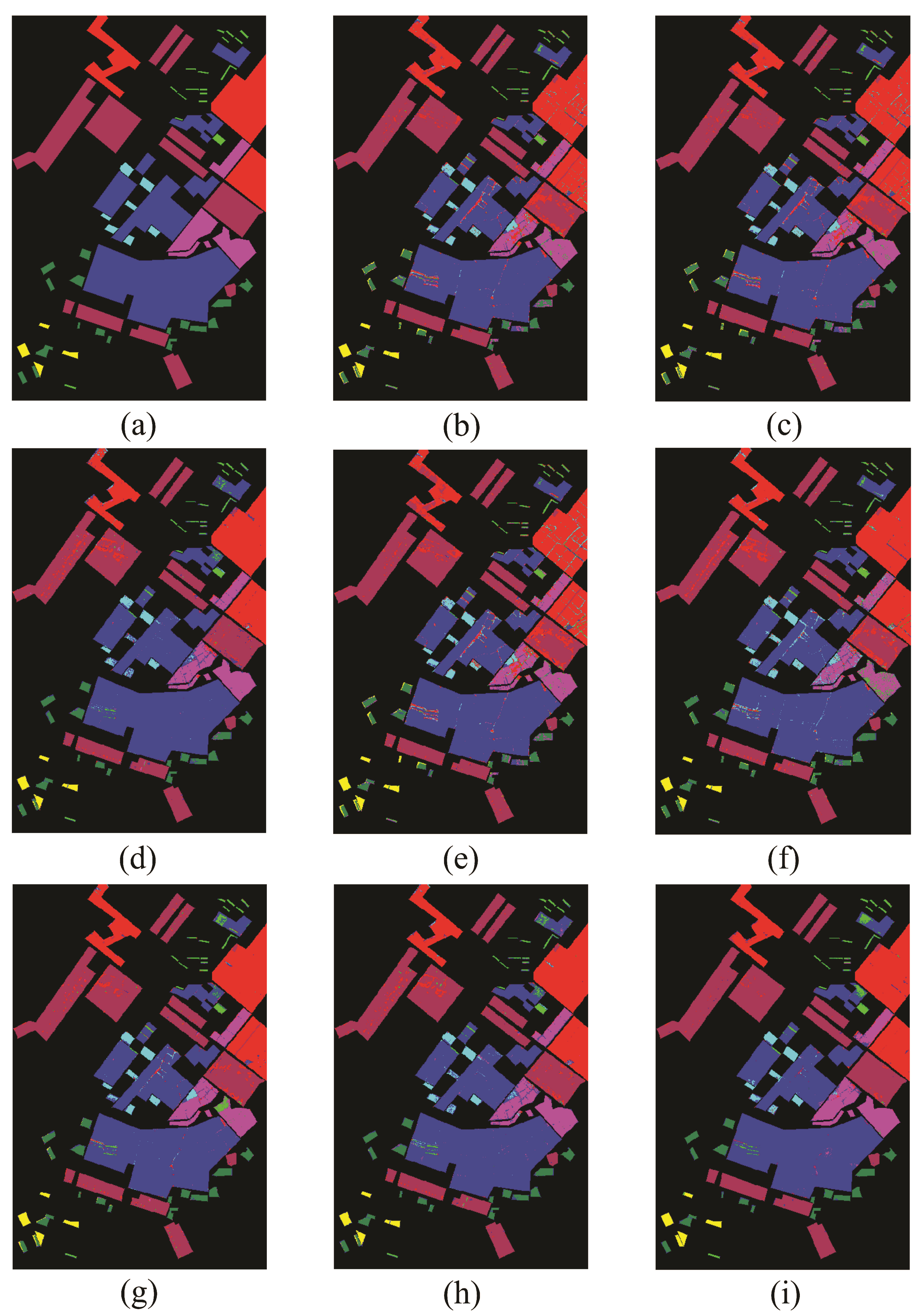
To further show the classification results of each class, 0.1% samples were randomly selected for training, and the rest were used as test samples. The classification results of different methods on the Heihe data set is shown in

Table 4. Classification results of each class samples via different DR methods in Heihe data set (%).

Class	Samples		DR with SVM Classifier
	Train	Test	Baseline	PCA	LDA	NPE	LPP	MFA	LGSFA	MFMDA
1	42	41029	96.23	95.87	98.49	97.33	98.07	97.64	98.56	97.86
2	29	28557	97.86	97.53	98.74	96.77	96.89	98.06	97.93	81.23
3	21	20334	95.46	95.26	97.24	95.27	95.77	96.54	95.45	95.66
4	10	7598	81.20	80.72	59.71	63.93	67.57	71.42	59.28	81.00
5	10	3752	84.81	84.21	72.62	84.03	73.25	78.11	72.79	83.31
6	10	1665	84.25	87.98	61.65	61.77	68.06	74.43	61.37	99.53
7	10	975	88.76	88.18	73.56	81.12	69.66	76.39	72.91	79.27
8	10	865	90.97	90.98	92.91	88.31	89.99	89.49	93.57	94.45
OA			94.72	94.45	93.71	93.09	93.40	94.31	93.14	95.64
AA			89.94	90.09	81.87	83.57	82.41	85.26	81.48	89.04
Kappa			0.93	0.92	0.92	0.91	0.90	0.91	0.92	0.94

Notes: The bold numbers represent the maximum OA of the row.

, and Figure 10 shows the corresponding classification maps.

As illustrated in Table 4, it can be concluded that the proposed method achieves good classification performance on many classes, such as Endive Sprout and Artificial Surfaces. In addition, it possesses a smoother classification map, which is more conductive to practical application scenarios.

4.6. Experiments on the PaviaU Data Set

In this section, we used PaviaU data set to analyze the classification performance of the proposed algorithm under different scenes. We randomly selected 40 samples per class as training set to explore OAs with respect to different parameters. The results are displayed in Figure 11.

In Figure 11a, as the increase of $n_w$, the OA rises first and then decreases slightly, the reason for this is that a small number of intraclass neighbor points cannot effectively explore intramanifold structure, while a large value of $n_w$ will include redundant information and lead to a decrease in classification accuracy. At the same time, when $n_b$ is lower than 8, the OAs can maintain a stable value. As shown in Figure 11b, the classification accuracy can fluctuate in a small range when the values of $\alpha$ and $\beta$ continue to increase. It shows that $\alpha$ and $\beta$ can balance the information between the intramanifold and intermanifold structures in HSI data. To achieve good classification performance, we selected $n_w$, $n_b$, $\alpha$ and $\beta$ as 28, 4, 0.5, 0.3, respectively.

To verify the effectiveness of the proposed algorithm, we randomly selected n${}_i$ (n${}_i$ = 5, 10, 20, 30, 40) samples from each class for training and remaining samples for testing. The average OAs with STD are given in

Table 5. Classification results using different methods with different classifiers for the PaviaU data set. [Overall Accuracy ± Std (%)].

	Algorithm	${\mathit{n}}_{\mathit{i}}$ = 5	${\mathit{n}}_{\mathit{i}}$ = 10	${\mathit{n}}_{\mathit{i}}$ = 20	${\mathit{n}}_{\mathit{i}}$ = 30	${\mathit{n}}_{\mathit{i}}$ = 40
	Baseline	57.16 ± 9.94	69.72 ± 4.19	78.07 ± 2.88	81.11 ± 3.91	82.97 ± 2.33
	PCA	57.16 ± 9.94	69.72 ± 4.19	78.01 ± 2.98	81.11 ± 3.91	83.13 ± 2.35
Spectral	LDA	53.09 ± 5.85	57.87 ± 3.84	65.79 ± 3.21	70.08 ± 3.11	74.14 ± 2.15
Features	NPE	57.64 ± 9.81	67.02 ± 4.68	73.50 ± 4.81	79.98 ± 3.71	81.54 ± 2.47
	LPP	49.70 ± 5.35	50.66 ± 5.65	66.37 ± 2.23	73.57 ± 1.53	75.84 ± 2.25
	MFA	62.24 ± 5.56	75.16 ± 3.27	77.51 ± 2.17	80.97 ± 2.70	82.26 ± 3.68
	LGSFA	57.38 ± 4.50	62.91 ± 3.32	69.37 ± 3.36	71.11 ± 2.37	75.97 ± 1.76
	Baseline	52.05 ± 8.27	72.01 ± 5.50	81.38 ± 2.22	86.32 ± 1.91	88.22 ± 1.21
	PCA	50.44 ± 7.55	67.93 ± 6.81	78.23 ± 3.68	81.71 ± 7.89	85.68 ± 2.42
LBP	LDA	60.31 ± 6.87	76.02 ± 2.59	82.54 ± 1.32	86.70 ± 1.27	88.88 ± 0.56
Features	NPE	55.73 ± 6.77	73.68 ± 5.81	75.50 ± 3.50	85.69 ± 2.68	86.45 ± 1.41
	LPP	43.22 ± 11.11	55.85 ± 13.49	76.32 ± 4.19	84.27 ± 3.10	85.03 ± 2.62
	MFA	57.35 ± 7.51	71.79 ± 4.28	81.39 ± 1.93	85.63 ± 2.69	86.86 ± 1.43
	LGSFA	63.02 ± 6.49	73.59 ± 3.66	81.54 ± 2.42	85.81 ± 2.66	86.75 ± 2.16
	Baseline	59.40 ± 5.75	68.29 ± 5.54	80.06 ± 4.65	83.93 ± 2.53	85.73 ± 2.31
	PCA	57.52 ± 10.11	70.67 ± 3.63	77.52 ± 6.12	82.69 ± 3.33	85.63 ± 1.87
Stacked	LDA	59.89 ± 5.94	76.62 ± 2.74	81.85 ± 2.89	85.14 ± 3.80	87.28 ± 2.22
Features	NPE	57.50 ± 10.99	75.35 ± 2.34	77.89 ± 3.47	84.53 ± 3.87	85.62 ± 2.73
	LPP	64.96 ± 6.68	71.29 ± 3.56	78.12 ± 3.83	86.07 ± 1.68	87.86 ± 1.92
	MFA	61.57 ± 8.86	74.61 ± 4.66	79.07 ± 2.08	81.58 ± 2.30	82.34 ± 2.66
	LGSFA	64.45 ± 4.72	78.79 ± 2.68	88.03 ± 2.26	92.94 ± 2.02	94.15 ± 1.42
MFMDA		78.70 ± 2.70	84.60 ± 2.34	92.66 ± 2.32	95.10 ± 1.84	96.09 ± 0.97

Notes: The bold numbers represent the maximum OA of the column.

.

It can be seen from Table 5, the OAs of each method are improved when more samples are used for training. MFMDA achieves better results than other algorithms in most cases, the reason is that it can increase the margins between different classes, so the discriminant features are obtained for classification.

To compare the classification performance of various DR methods, we randomly selected 1% data in each class for training, and remaining data were used as test samples. As shown in Table 5, LBP features and stacked features achieve better experiment results than spectral features, so we choose stacked features compared with the MFMDA method.

Table 6. Classification results of each class samples via different DR methods in PaviaU data set (%).

Class	Samples		DR with SVM Classifier
	Train	Test	Baseline	PCA	LDA	NPE	LPP	MFA	LGSFA	MFMDA
1	10	6565	89.98	89.77	92.95	89.24	93.72	90.37	92.43	97.90
2	186	18463	97.93	97.41	98.04	97.63	98.03	97.46	97.27	99.79
3	21	2078	72.28	69.59	75.81	68.50	73.39	69.82	77.02	94.02
4	31	3033	85.50	85.32	89.52	85.38	87.94	86.74	89.10	84.89
5	13	1332	98.97	98.84	99.65	98.74	99.29	99.41	99.64	99.99
6	50	4979	85.45	80.95	84.26	83.02	80.26	80.16	80.90	99.14
7	13	1317	81.97	76.74	67.06	78.02	67.56	74.68	69.35	96.10
8	37	3645	85.48	84.37	86.75	83.81	89.99	84.82	88.13	98.06
9	10	937	99.73	99.68	94.26	99.75	99.86	99.79	99.61	60.91
OA			91.59	90.39	91.96	90.59	91.78	90.52	91.49	96.95
AA			88.59	86.96	87.59	87.12	87.78	87.03	88.16	92.31
Kappa			0.89	0.87	0.89	0.87	0.89	0.87	0.89	0.96

Notes: The bold numbers represent the maximum OA of the row.

gives the classification accuracies of different methods and Figure 12 shows the corresponding classification maps.

As shown in Table 6, the proposed method obtained the best classification results in most classes, especially in Asphalt, Gravel, Bare Soil, Bitumen, Bricks. The reason is that the MFMDA algorithm effectively fuses the multiple features by compacting spectral features and LBP features from the same class in low-dimensional space. As displayed in Figure 12, MFMDA algorithm has fewer misclassified points and the classification map is smoother than other methods.

4.7. Discussion

The experiments on three HSI data sets reveal some interesting points.

• As shown in Table 1, Table 3 and Table 5, the classification performance of simply stacked features is even worse than LBP features in most cases, for the reason that simply stacked spatial and spectral features may yield redundant information and even lead to the curse-of-dimensionality.
• From the experimental results, it is obviously that DR methods on LBP features or spectral features usually perform better than DR methods on the simply stacked features. This may be due to the fact that performing dimensionality reduction directly on the simply stacked features cannot reveal the manifold structure of different features in HSI, which will restrict their discriminant capability for classification.
• The proposed MFMDA algorithm is superior to other DR methods under different training conditions. The reason is that MFMDA constructs the intrinsic graphs and penalty graphs of spectral features and LBP features to discover the manifold structure of spatial features and spectral features, then it learns low-dimensional embedding space from original spectral features as well as LBP features for compacting the intramanifold samples while separating intermanifold samples. As a result, the spatial-spectral embedding features possess stronger discriminating ability for HSI classification.

5. Conclusions

Traditional methods explore only a single feature or simply stacked features in hyperspectral image, which will restrict their discriminant capability for classification. In this paper, we proposed a new dimensionality reduction method termed MFMDA to couple DR and fusion of spectral and textual features of HSI data. MFMDA first explores LBP operator to extract textural features for encoding the spatial information in HSI. Then, within GE framework, the intrinsic and penalty graphs of LBP and spectral features are constructed to explore the discriminant manifold structure in both spatial and spectral domains, respectively. After that, a new spatial-spectral DR model is built to extract discriminant spatial-spectral combined features which not only preserve the similarity relationship between spectral features and LBP features but also possess strong discriminating ability in the low-dimensional embedding space. Experiments on Indian Pines, Heihe and PaviaU hyperspectral data sets demonstrate that the proposed MFMDA method can significantly improve classification performance and result in smoother classification maps than some state-of-the-art methods, and with fewer training samples, the classification accuracy can reach 95.43%, 97.19% and 96.60%, respectively. In the future, we will focus on conducting a more detailed investigation of other possible features to further improve the performance of MFMDA.

References

- Song, W.W.; Li, S.T.; Fang, L.Y.; Lu, T. Hyperspectral Image Classification With Deep Feature Fusion Network. IEEE Trans. Geosci. Remote Sens. 2016, 54, 4544–4554. [Google Scholar] [CrossRef]
- Zhong, Y.F.; Wang, X.Y.; Xu, Y.; Wang, S.Y.; Jia, T.Y.; Hu, X.; Zhao, J.; Wei, L.F.; Zhang, L.P. Mini-UAV-Borne Hyperspectral Remote Sensing: From Observation and Processing to Applications. IEEE Geosci. Remote Sens. Mag. 2018, 6, 46–62. [Google Scholar] [CrossRef]
- Chen, Y.S.; Jiang, H.L.; Li, C.Y.; Jia, X.P.; Ghamisi, P. Deep Feature Extraction and Classification of Hyperspectral Images Based on Convolutional Neural Networks. IEEE Trans. Geosci. Remote Sens. 2016, 54, 6232–6251. [Google Scholar] [CrossRef]
- Huang, H.; Duan, Y.L.; Shi, G.Y.; Lv, Z.Y. Fusion of Weighted Mean Reconstruction and SVMCK for Hyperspectral Image Classification. IEEE Access 2018, 6, 15224–15235. [Google Scholar] [CrossRef]
- Sun, W.W.; Yang, G.; Wu, K.; Li, W.Y.; Zhang, D.F. Pure endmember extraction using robust kernel archetypoid analysis for hyperspectral imagery. ISPRS J. Photogramm. Remote Sens. 2017, 131, 147–159. [Google Scholar] [CrossRef]
- Jiao, C.Z.; Chen, C.; McGarvey, R.G.; Bohlman, S.; Jiao, L.C.; Zare, A. Multiple Instance Hybrid Estimator for Hyperspectral Target Characterization and Sub-pixel Target Detection. J. Photogramm. Remote Sens. 2018, 146, 235–250. [Google Scholar] [CrossRef]
- Dian, R.W.; Li, S.T.; Guo, A.J.; Fang, L.Y. Deep Hyperspectral Image Sharpening. IEEE Trans. Neural Netw. Learn. Syst. 2018, 29, 5345–5355. [Google Scholar] [CrossRef] [PubMed]
- Wang, X.Y.; Zhong, Y.F.; Xu, Y.; Zhang, L.P.; Xu, Y.Y. Saliency-Based Endmember Detection for Hyperspectral Imagery. IEEE Trans. Geosci. Remote Sens. 2018, 56, 3667–3680. [Google Scholar] [CrossRef]
- Wang, Q.; Lin, J.Z.; Yuan, Y. Salient Band Selection for Hyperspectral Image Classification via Manifold Ranking. IEEE Trans. Neural Netw. Learn. Syst. 2016, 27, 1279–1289. [Google Scholar] [CrossRef] [PubMed]
- Qian, Y.T.; Xiong, F.C.; Zeng, S.; Zhou, J.; Tang, Y.Y. Matrix-Vector Nonnegative Tensor Factorization for Blind Unmixing of Hyperspectral Imagery. IEEE Trans. Geosci. Remote Sens. 2017, 55, 1776–1792. [Google Scholar] [CrossRef]
- Luo, F.L.; Huang, H.; Liu, J.M.; Ma, Z.Z. Fusion of Graph Embedding and Sparse Representation for Feature Extraction and Classification of Hyperspectral Imagery. Photogramm. Eng. Remote Sens. 2017, 83, 37–46. [Google Scholar] [CrossRef]
- Kang, X.D.; Duan, P.H.; Li, S.T.; Benediktsson, J.A. Decolorization-Based Hyperspectral Image Visualization. IEEE Trans. Geosci. Remote Sens. 2018, 56, 4346–4360. [Google Scholar] [CrossRef]
- Ke, W.; Xu, G.; Zhang, Y.X.; Du, B. Hyperspectral image target detection via integrated background suppression with adaptive weight selection. Neurocomputing 2017, 315, 59–67. [Google Scholar]
- Xu, Y.H.; Zhang, L.P.; Du, B.; Zhang, F. Spectral-Spatial Unified Networks for Hyperspectral Image Classification. IEEE Trans. Geosci. Remote Sens. 2018, 56, 5893–5909. [Google Scholar] [CrossRef]
- Li, S.T.; Hao, Q.B.; Kang, X.D.; Benediktsson, J.A. Gaussian Pyramid Based Multiscale Feature Fusion for Hyperspectral Image Classification. IEEE J. Sel. Top. Appl. Earth Obs. Remote Sens. 2018, 11, 3312–3324. [Google Scholar] [CrossRef]
- Peng, J.T.; Li, L.Q.; Tang, Y.Y. Maximum Likelihood Estimation-Based Joint Sparse Representation for the Classification of Hyperspectral Remote Sensing Images. IEEE Trans. Neural Netw. Learn. Syst. 2018, 1–13. [Google Scholar] [CrossRef]
- Wang, Z.M.; Du, B.; Zhang, L.F.; Zhang, L.P.; Jia, X.P. A Novel Semisupervised Active-Learning Algorithm for Hyperspectral Image Classification. IEEE Trans. Geosci. Remote Sens. 2017, 55, 3071–3083. [Google Scholar] [CrossRef]
- Su, H.J.; Zhao, B.; Du, Q.; Sheng, Y.H. Tangent Distance-Based Collaborative Representation for Hyperspectral Image Classification. IEEE Geosci. Remote Sens. Lett. 2016, 13, 1236–1240. [Google Scholar] [CrossRef]
- Zhang, L.F.; Zhang, L.P.; Tao, D.C.; Huang, X. On Combining Multiple Features for Hyperspectral Remote Sensing Image Classification. IEEE Trans. Geosci. Remote Sens. 2012, 50, 879–893. [Google Scholar] [CrossRef]
- Liao, W.Z.; Mura, M.D.; Chanussot, J.; Pizurica, A. Fusion of spectral and spatial information for classification of hyperspectral remote sensed imagery by local graph. IEEE J. Sel. Top. Appl. Earth Obs. Remote Sens. 2018, 9, 583–594. [Google Scholar] [CrossRef]
- Su, H.J.; Zhao, B.; Du, Q.; Du, P.J.; Xue, Z.H. Multifeature Dictionary Learning for Collaborative Representation Classification of Hyperspectral Imagery. IEEE Trans. Geosci. Remote Sens. 2018, 56, 2467–2484. [Google Scholar] [CrossRef]
- Fang, L.Y.; Li, S.T.; Duan, W.H.; Ren, J.C.; Benediktsson, J.A. Classification of Hyperspectral Images by Exploiting Spectral-Spatial Information of Superpixel via Multiple Kernels. IEEE Trans. Geosci. Remote Sens. 2015, 53, 6663–6674. [Google Scholar] [CrossRef]
- Liang, M.M.; Jiao, L.C.; Yang, S.Y.; Liu, F.; Hou, B.; Chen, H. Deep Multiscale Spectral-Spatial Feature Fusion for Hyperspectral Images Classification. IEEE J. Sel. Top. Appl. Earth Obs. Remote Sens. 2018, 11, 2911–2924. [Google Scholar] [CrossRef]
- Chen, C.; Li, W.; Su, H.J.; Liu, K. Spectral-Spatial Classification of Hyperspectral Image Based on Kernel Extreme Learning Machine. Remote Sens. 2014, 6, 5795–5814. [Google Scholar] [CrossRef]
- Gu, Y.F.; Liu, T.Z.; Jia, X.P.; Benediktsson, J.A.; Chanussot, J. Nonlinear Multiple Kernel Learning With Multiple-Structure-Element Extended Morphological Profiles for Hyperspectral Image Classification. IEEE Trans. Geosci. Remote Sens. 2016, 54, 3235–3247. [Google Scholar] [CrossRef]
- Zhao, W.Z.; Du, S.H. Spectral-Spatial Feature Extraction for Hyperspectral Image Classification: A Dimension Reduction and Deep Learning Approach. IEEE Trans. Geosci. Remote Sens. 2016, 54, 4544–4554. [Google Scholar] [CrossRef]
- Luo, F.L.; Du, B.; Zhang, L.P.; Zhang, L.F.; Tao, D.C. Feature Learning Using Spatial-Spectral Hypergraph Discriminant Analysis for Hyperspectral Image. IEEE Trans. Cybern. 2018. [Google Scholar] [CrossRef]
- Zhang, X.R.; Gao, Z.Y.; Jiao, L.C.; Zhou, H.Y. Multifeature Hyperspectral Image Classification with Local and Nonlocal Spatial Information via Markov Random Field in Semantic Space. IEEE Trans. Geosci. Remote Sens. 2018, 56, 1409–1424. [Google Scholar] [CrossRef]
- Li, W.; Chen, C.; Su, H.J.; Du, Q. Local Binary Patterns and Extreme Learning Machine for Hyperspectral Imagery Classification. IEEE Trans. Geosci. Remote Sens. 2015, 55, 3681–3693. [Google Scholar] [CrossRef]
- Mauro, M.D.; Benediktsson, J.A.; Waske, B.; Bruzzone, L. Morphological Attribute Profiles for the Analysis of Very High Resolution Images. IEEE Trans. Geosci. Remote Sens. 2010, 48, 3747–3762. [Google Scholar]
- Li, J.; Marpu, P.R.; Plaza, A.; Bioucas-Dias, J.M.; Benediktsson, J.A. Generalized Composite Kernel Framework for Hyperspectral Image Classification. IEEE Trans. Geosci. Remote Sens. 2013, 51, 4816–4839. [Google Scholar] [CrossRef]
- Li, J.; Huang, X.; Gamba, P.; Bioucas-Dias, J.M.; Zhang, L.P.; Benediktsson, J.A.; Plaza, A. Multiple Feature Learning for Hyperspectral Image Classification. IEEE Trans. Geosci. Remote Sens. 2015, 53, 1592–1606. [Google Scholar] [CrossRef]
- Song, C.Y.; Yang, F.J.; Li, P.J. Rotation invariant texture measured by local binary pattern for remote sensing image classification. In Proceedings of the 2010 Second International Workshop on Education Technology and Computer Science, Wuhan, China, 6–7 March 2010; Volume 3, pp. 3–6. [Google Scholar]
- Zhong, Y.F.; Ma, A.; Ong, Y.S.; Zhu, Z.X.; Zhang, L.P. Computational intelligence in optical remote sensing image processing. Appl. Soft Comput. 2018, 64, 75–93. [Google Scholar] [CrossRef]
- Xu, J.; Yang, G.; Yin, Y.F.; Man, H.; He, H.B. Sparse Representation Based Classification with Structure Preserving Dimension Reduction. Cogn. Comput. 2014, 6, 608–621. [Google Scholar] [CrossRef]
- Wang, J.; He, H.B.; Prokhorov, D.V. A Folded Neural Network Autoencoder for Dimensionality Reduction. Proc. Comput. Sci. 2012, 13, 120–127. [Google Scholar] [CrossRef]
- Zhou, Y.C.; Peng, J.T.; Chen, C.L.P. Dimension Reduction Using Spatial and Spectral Regularized Local Discriminant Embedding for Hyperspectral Image Classification. IEEE Trans. Geosci. Remote Sens. 2015, 53, 1082–1095. [Google Scholar] [CrossRef]
- Zheng, X.T.; Yuan, Y.; Lu, X.Q. Dimensionality Reduction by Spatial-Spectral Preservation in Selected Bands. IEEE Trans. Geosci. Remote Sens. 2017, 55, 5185–5197. [Google Scholar] [CrossRef]
- Bonifazi, G.; Capobianco, G.; Serranti, S. Asbestos containing materials detection and classification by the use of hyperspectral imaging. J. Hazard. Mater. 2018, 13, 981–993. [Google Scholar] [CrossRef] [PubMed]
- Huang, X.Y.; Zhang, B.; Qiao, H.; Nie, X.L. Local Discriminant Canonical Correlation Analysis for Supervised PolSAR Image Classification. IEEE Geosci. Remote Sens. Lett. 2017, 14, 2102–2106. [Google Scholar] [CrossRef]
- Xu, X.; Huang, Z.H.; Zuo, L.; He, H.B. Manifold-based Reinforcement Learning via Locally Linear Reconstruction. IEEE Trans. Neural Netw. Learn. Syst. 2012, 28, 934–947. [Google Scholar] [CrossRef] [PubMed]
- Li, W.; Zhang, L.P.; Zhang, L.F.; Du, B. GPU Parallel Implementation of Isometric Mapping for Hyperspectral Classification. IEEE Geosci. Remote Sens. Lett. 2017, 14, 1532–1539. [Google Scholar] [CrossRef]
- Xu, X.; Yang, H.Y.; Lian, C.Q.; Liu, J.H. Self-learning control using dual heuristic programming with global Laplacian eigenmaps. IEEE Trans. Ind. Electron. 2017, 64, 9517–9526. [Google Scholar] [CrossRef]
- Deng, Y.J.; Li, H.C.; Pan, L.; Shao, L.Y.; Du, Q.; Emery, W.J. Modified Tensor Locality Preserving Projection for Dimensionality Reduction of Hyperspectral Images. IEEE Geosci. Remote Sens. Lett. 2018, 15, 277–281. [Google Scholar] [CrossRef]
- Zhang, L.L.; Zhao, C.H. Sparsity divergence index based on locally linear embedding for hyperspectral anomaly detection. J. Appl. Remote Sens. 2016, 10, 025026. [Google Scholar] [CrossRef]
- Lu, G.F.; Jin, Z.; Zou, J. Face recognition using discriminant sparsity neighborhood preserving embedding. Knowl. Based Syst. 2012, 31, 119–127. [Google Scholar] [CrossRef]
- Wang, J.; Sun, X.L.; Du, J.X. Local tangent space alignment via nuclear norm regularization for incomplete data. Neurocomputing 2018, 273, 141–151. [Google Scholar] [CrossRef]
- Lu, Y.W.; Lai, Z.H.; Fan, Z.Z.; Cui, J.R.; Zhu, Q. Manifold discriminant regression learning for image classification. Neurocomputing 2015, 166, 475–486. [Google Scholar] [CrossRef]
- Yu, H.Y.; Gao, L.R.; Li, W.; Du, Q.; Zhang, B. Locality sensitive discriminant analysis for group sparse representation-based hyperspectral imagery classification. IEEE Geosci. Remote Sens. Lett. 2017, 14, 1358–1362. [Google Scholar] [CrossRef]
- Jiang, J.J.; Hu, R.M.; Wang, Z.Y.; Cai, Z.H. CDMMA: Coupled discriminant multi-manifold analysis for matching low-resolution face images. Signal Process. 2016, 124, 162–172. [Google Scholar] [CrossRef]
- Luo, F.L.; Huang, H.; Duan, Y.L.; Liu, J.M.; Liao, Y.H. Local geometric structure feature for dimensionality reduction of hyperspectral imagery. Remote Sens. 2017, 9, 790. [Google Scholar] [CrossRef]
- Fauvel, M.; Benediktsson, J.A.; Chanussot, J.; Sveinsson, J.R. Spectral and Spatial Classification of Hyperspectral Data Using SVMs and Morphological Profile. IEEE Trans. Geosci. Remote Sens. 2018, 9, 3804–3814. [Google Scholar]
- Huo, L.Z.; Tang, P. Spectral and spatial classification of hyperspectral data using SVMs and Gabor textures. Proc. Int. Geosci. Remote Sens. Symp. 2011, 9, 1708–1711. [Google Scholar]
- Huang, K.S.; Li, S.T.; Kang, X.D.; Fang, L.Y. Spectral-spatial hyperspectral image classification based on KNN. Sens. Imaging 2016, 17, 1. [Google Scholar] [CrossRef]
- Xiao, Q.; Wen, J.G. HiWATER: Thermal-Infrared Hyperspectral Radiometer (4th, July, 2012). Heihe Plan Sci. Data Center 2013. [Google Scholar] [CrossRef]
- Xue, Z.H.; Su, H.J.; Du, P.J. Sparse graph regularization for robust crop mapping using hyperspectral remotely sensed imagery: A case study in Heihe Zhangye oasis. In Proceedings of the 2016 IEEE International Geoscience and Remote Sensing Symposium (IGARSS), Beijing, China, 10–15 July 2016; pp. 779–782. [Google Scholar]
- Chang, C.C.; Lin, C.J. LIBSVM: A library for support vector machines. ACM Trans. Intell. Syst. Technol. 2011, 2, 475–486. [Google Scholar] [CrossRef]
- Chang, C.C.; Lin, C.J. LIBSVM: Perceptual Image Hashing Using Latent Low-Rank Representation and Uniform LBP. Appl. Sci. 2018, 8, 317. [Google Scholar]
Figure 1.
The procedure of local binary patterns (LBP) operator on the PaviaU image.
Figure 2.
The flowchart of multi-feature manifold discriminant analysis.
Figure 3.
Indian Pines hyperspectral image. (a) HSI in false-color (bands 50, 27 and 17 for RGB); (b) Ground-truth map (please note that the number of samples is given in parentheses).
Figure 4.
Heihe hyperspectral image. (a) HSI in false-color (bands 57, 19 and 80 for RGB); (b) Ground-truth map (please note that the number of samples is given in parentheses).
Figure 5.
PaviaU hyperspectral image. (a) HSI in false-color (bands 60, 100 and 20 for RGB); (b) Ground-truth map (please note that the number of samples is given in parentheses).
Figure 6.
Classification results with different dimensions on the Indian Pines, Heihe and PaviaU data sets. (a) Indian Pines; (b) Heihe; (c) PaviaU.
Figure 7.
The experiments for parameter analysis of MFMDA on Indian Pines data set. (a) Classification results of MFMDA with different values of and ; (b) Classification results of MFMDA with different parameters and .
Figure 8.
Classification results of different algorithms on Indian pines data set. (a) Ground truth; (b) Baseline(93.57%, 0.93); (c) PCA(92.57%, 0.92); (d) LDA(93.43%, 0.92); (e) NPE(92.29%, 0.91); (f) LPP(92.43%, 0.91); (g) MFA(92.78%, 0.92); (h) LGSFA(92.72%, 0.92); (i) MFMDA(95.71%, 0.95). Please note that OA and k coefficients are given in parentheses.
Figure 9.
The experiments for parameter analysis of MFMDA on Heihe data set. (a) OAs of MFMDA with different values of and ; (b) OAs of MFMDA with different values of and .
Figure 10.
Classification results of different algorithms on Heihe data set. (a) Ground truth; (b) Baseline (94.72%, 0.93); (c) PCA (94.45%, 0.92); (d) LDA (93.71%, 0.92); (e) NPE (93.09%, 0.91); (f) LPP (93.40%, 0.90); (g) MFA (94.31%, 0.91); (h) LGSFA (93.14%, 0.92); (i) MFMDA (95.64%, 0.94). Please note that OA and k coefficients are given in parentheses.
Figure 11.
The experiments for parameter analysis of MFMDA on PaviaU data set. (a) Classification results of MFMDA with different parameters of and ; (b) Classification results of MFMDA with different parameters and .
Figure 12.
Classification results of different algorithms on PaviaU data set. (a) Ground truth; (b) Baseline(91.59%, 0.89); (c) PCA(90.39%, 0.87); (d) LDA(91.96%, 0.89); (e) NPE(90.59%, 0.87); (f) LPP(91.78%, 0.89); (g) MFA(90.52%, 0.87); (h) LGSFA(91.49%, 0.89); (i) MFMDA(96.95%, 0.96). Please note that OA and k coefficients are given in parentheses.