Machine Learning Techniques for Tree Species Classification Using Co-Registered LiDAR and Hyperspectral Data

1
Department of Earth & Environment, Boston University, Boston, MA 02215, USA
2
Department of Geography and Environmental Science, Hunter College of the City of New York, New York, NY 10065, USA
*
Author to whom correspondence should be addressed.
Remote Sens. 2019, 11(7), 819; https://0-doi-org.brum.beds.ac.uk/10.3390/rs11070819
Submission received: 13 February 2019
/
Revised: 29 March 2019
/
Accepted: 1 April 2019
/
Published: 5 April 2019
(This article belongs to the Special Issue Advances in Remote Sensing of Forest Structure and Applications)
Abstract
:The use of light detection and ranging (LiDAR) techniques for recording and analyzing tree and forest structural variables shows strong promise for improving established hyperspectral-based tree species classifications; however, previous multi-sensoral projects were often limited by error resulting from seasonal or flight path differences. The National Aeronautics and Space Administration (NASA) Goddard’s LiDAR, hyperspectral, and thermal imager (G-LiHT) is now providing co-registered data on experimental forests in the United States, which are associated with established ground truths from existing forest plots. Free, user-friendly machine learning applications like the Orange Data Mining Extension for Python recently simplified the process of combining datasets, handling variable redundancy and noise, and reducing dimensionality in remotely sensed datasets. Neural networks, CN2 rules, and support vector machine methods are used here to achieve a final classification accuracy of 67% for dominant tree species in experimental plots of Howland Experimental Forest, a mixed coniferous–deciduous forest with ten dominant tree species, and 59% for plots in Penobscot Experimental Forest, a mixed coniferous–deciduous forest with 15 dominant tree species. These accuracies are higher than those produced using LiDAR or hyperspectral datasets separately, suggesting that combined spectral and structural data have a greater richness of complementary information than either dataset alone. Using greatly simplified datasets created by our dimensionality reduction methodology, machine learner performance remains comparable or higher to that using the full dataset. Across forests, the identification of shared structural and spectral variables suggests that this methodology can successfully identify parameters with high explanatory power for differentiating among tree species, and opens the possibility of addressing large-scale forestry questions using optimized remote sensing workflows.
1. Introduction
The use of geographic information systems (GIS) and remote sensing techniques for forestry applications has been a major concern in the field of geography since its creation, and a technical revolution in the last three decades allowed for increasingly sophisticated analysis of forest structure, composition, and dynamics. Although optical, multispectral, and hyperspectral remote-sensing techniques are traditionally used to gather data on forests, the incorporation of data on tree and canopy structure can improve analysis of forest biomass and health, carbon sequestration potential, and range, potentially even at the species level [1]. Light detection and ranging (LiDAR) technologies are increasingly being employed to collect data on structural features of tree canopies and branching patterns, forest structure and succession, and even estimates of tree physiological metrics such as leaf area index [2]. The use of LiDAR sensors, usually on airborne platforms such as small airplanes, also proved to be a boon to commercial forest resource monitoring and valuation. The ability to accurately estimate the height and other forest parameters, such as basal area or timber volume, with a single flyover greatly simplified the valuation of forests grown for timber [3].
Changing weather patterns will reshape the ranges of species worldwide, and the ability to monitor the changes in community dynamics of trees and other plants, which play a fundamental role in overall ecosystem functioning and composition, will be key in understanding trends in terrestrial biomes and in creating effective strategies for conservation, resilience, and human livelihoods [4]. Whether a forest is assessed for conservation or commercial purposes, one key element of forest systems remains difficult to quantify; individual LiDAR data points have little to say about the species identity of a given tree. Nonetheless, tree species differ in their canopy architecture, overall shape factor, and foliage type; such morphological characteristics were used as the basis for LiDAR-based differentiation between deciduous and coniferous trees [5] and for more detailed species-level classifications [6,7,8]. When collecting LiDAR data, a single laser pulse may be reflected off multiple canopy structures and recorded as several returns with different light intensities [9]. Full-waveform LiDAR datasets contain information on these multiple within-canopy echoes and, thus, provide robust information on complex canopy architecture and forest composition. In addition to species-level classification, such datasets were used to estimate additional forest biomass parameters [10]. However, discrete-return LiDAR data were found to provide additional information on forest structure beyond that provided by full-waveform LiDAR data [11], and can offer valuable insight into tree and forest canopies, for example, by using summary metrics calculated by binning a LiDAR point cloud into percentiles, deciles, or other values summarizing individual ground and canopy returns [12]. Similar structural indices were used with success when surveying vegetation biodiversity [13], and it is, thus, possible to take advantage of high-density LiDAR data to examine branching patterns and other architectural data on a single-tree or tree-stand basis, and to relate this to the species of individual trees or of the predominant species in a stand.
The structural information provided by discrete-return LiDAR was used with success to characterize species richness [14] and predict species composition of individual stands [15] in tropical forests, and to differentiate among tree species or taxonomic groups [16,17,18]. Classifications attempted on forests with only a few tree species [19] and those using a high density of LiDAR points [20,21,22] have achieved high accuracies; however, the utility of LiDAR summary metrics was more limited when attempting to extend similar classifications to a larger number of tree species [23]. Additionally, debate continues over the optimal resolution of LiDAR data in comparison to individual tree crown size. Some researchers warned against trying to create species-level maps with data coarser than the individual tree level [24], although others asserted that there is unavoidable within-species variability due to an individual-tree signature that explains up 65% of intraspecies variability [25]. While some researchers had success in performing individual tree detection (ITD) to closely approximate the location and size of trees and tree crowns [26,27], ITD remains a field with uncertainties that will need to be addressed before it can be implemented for robust forest inventory or valuation [28]. Until such methods are perfected, it remains prudent to work at the scale of aggregated tree stands, plots, or groups for large-scale forest inventory or classification when using discrete-return LiDAR data.
In addition to the structural information offered by LiDAR datasets, remote tree species classifications may take advantage of the differential reflectance of different wavelengths of light within heterogeneous forest canopies. Multispectral [29,30] and optical [31,32] datasets were previously used in combination with LiDAR for species-level classifications, and hyperspectral data in particular were used for tree species classification because of the differences in light reflectance off leaves with species-specific pigment concentrations [33]. Using a similar principle, recently developed multispectral LiDAR systems can be used to gather wavelength-dependent structural information, and were used for tree species identification with higher accuracies than single-wavelength LiDAR data [34,35,36,37]. The use of LiDAR data to identify gaps in the tree canopy also bolstered the accuracy of some hyperspectral classifications [38,39,40]. Fused hyperspectral and LiDAR datasets also show promise for ecological problems other than species classification, including biomass estimation [41], habitat characterization [42], and forest fire risk evaluation [43]. Very few studies (with the exception of Reference [44]) had the opportunity to use a co-registered hyperspectral and LiDAR dataset.
Recently available sensors like the National Aeronautics and Space Administration (NASA) Goddard’s LiDAR, hyperspectral, and thermal (G-LiHT) imager are helping to improve the utility and viability of projects combining LiDAR and hyperspectral data by providing co-registered data on established experimental forests [45]. These G-LiHT flights provide a double benefit for investigating advances in the remote sensing of vegetation. Firstly, co-registered data are historically a rarity in multi-sensoral projects, but are desirable because of the potential for reducing error resulting from seasonal or flight path differences. Secondly, the use of experimental forests as ground truth areas for remote-sensing projects is recommended because of the existing knowledge on the management of such areas and the possibility for connecting results of remote-sensing analyses to other existing research [46].
Datasets collected by G-LiHT also provide an excellent opportunity for evaluating new analytical methods. Remotely sensed datasets are often constrained or complicated by variable redundancy and noise, and traditional dimensionality reduction techniques require the use of computationally intense and expensive software programs. Additionally, most remotely sensed datasets, particularly hyperspectral ones, are very large. Given that only a fixed number of ground-truth sites or pixels typically exist for a particular project, this dimensionality leads to problems such as the Hughes phenomenon, where hyperspectral data on a forest for which the researcher has data on only a small number of ground truth areas might be more redundant than insightful [47]. For this reason, machine learning and data mining techniques for dimensionality reduction and pattern finding are often employed in species classification studies, as well as for predictive models of species distributions or habitat suitability [46,48,49,50,51,52], and they show strong promise for use in future work.
Large datasets like those collected by G-LiHT represent a classic case of the Hughes phenomenon and, therefore, an ideal opportunity to assess dimensionality reduction techniques. Previous researchers recommended techniques such as data filtering (retaining only a subset of a dataset for analysis, such as by removing incomplete cases or irrelevant variables), factor analysis, or separability indices used to reduce a large dataset to only the most informative subset, with the goal of improving the efficiency of machine learners and reducing correlation among variables used for classifier training [53]. Variables may be selected using parametric [54] or nonparametric [55] statistical methods, as well as more complex statistical methods aimed at variable selection, grouping [56], or iterative inter-comparisons of potential variable combinations for accurate and parsimonious model creation [57,58]. Additionally, machine learning methods, including random forests and support vector machines, were used as tools for pattern recognition and variable selection when working with large datasets [59,60]. It is becoming increasingly easy to implement such techniques; free, user-friendly data mining and machine learning applications like the Orange Data Mining Extension for Python (Orange) [61] recently simplified the process of combining and analyzing remotely sensed datasets for researchers at all levels. Thus, it is clear that there exist datasets and techniques that are ideally suited to respond to a need for optimized dimensionality reduction techniques, particularly as the collection of large datasets is becoming increasingly common in forest ecosystems. Here, we describe a methodology for assessing a suite of LiDAR and optical metrics refined by machine learning techniques to perform species-level tree classifications that optimize the contribution of both structural and spectral information.
2. Materials and Methods
2.1. Data Collection
The G-LiHT imager is composed of several compatible off-the-shelf navigation, spectrometry, imaging, and laser sensor products [45]. Flyovers relevant to this study were conducted in June 2012 and all data can be found in the G-LiHT data archive at ftp://fusionftp.gsfc.nasa.gov/G-LiHT. Discrete-return LiDAR data, originally collected at a density of six returns per square meter, are available in raster format, in which returns are aggregated to 13-m2 pixels (see Section 2.2 and Table 1 for more details); hyperspectral data are available at a 1-m2 resolution. In total, 190 individual variables are available as part of the G-LiHT outputs for each forest (32 LiDAR metrics, 114 hyperspectral reflectance bands, and 44 vegetation indices).
To complement G-LiHT data, NASA-funded field campaigns to Penobscot Experimental Forest and Howland Experimental Forest in Maine, United States of America (USA) in the summer of 2009 surveyed trees in the same experimental forests as the flyovers, generating species-level information on trees in ground truth areas. Howland Experimental Forest is a 225-ha forest with a centroid at 45°12′ north (N), 68°44′ west (W). Penobscot Experimental Forest is an approximately 1578-ha forest with a centroid at 44°85′20′′N, 68°62′00′′W. Both sites are mixed coniferous–deciduous, predominantly evergreen forests. Data were collected in forest plots (11 plots in Howland Experimental Forest and 12 plots in Penobscot Experimental Forest) of 50 m × 200 m, each of which was divided into 16 subplots of approximately 25 m × 25 m. Data on the species, tree height, and diameter at breast height (DBH) were recorded for each tree above 10 cm in DBH in these plots [62].
2.2. Data Preparation and Exploration
Binned point clouds generated by G-LiHT’s scanning LiDAR sensor were processed into standard metrics (as described in previous publications [63,64]; definitions in Table 1), available as raster files with 13-m2 resolution.
Available hyperspectral data include at-sensor reflectance data covering a spectrum between 418 and 918 nm, with an approximately 4.4-nm interval between bands for a total of 114 individual bands. A total of 44 different vegetation indices calculated from these reflectance measurements are also available (a select list for those discussed in this article are shown in Table 2).
To prepare these available data for analysis, a dominant species for each whole plot and subplot was determined and associated with subplot polygons (Table 3). Howland Experimental Forest was largely undisturbed in the 140 years since its establishment [83]. In Penobscot Experimental Forest, plots used in this analysis were outside areas used in cutting and forest management studies [84], and only minor disturbance from spruce budworm was reported [85]. Since forest age and tree size distributions can be assumed to be relatively stable in these areas, and because trees under 10 cm in DBH were already removed from analysis, the species with the greatest number of individual trees (stem count) was chosen as representative of the subplot-level dominant species. In four cases of a tie between two or more species, the species that was dominant in a neighboring subplot or throughout the entire plot was chosen.
2.3. Machine Learning Methods, Accuracy, and Validation
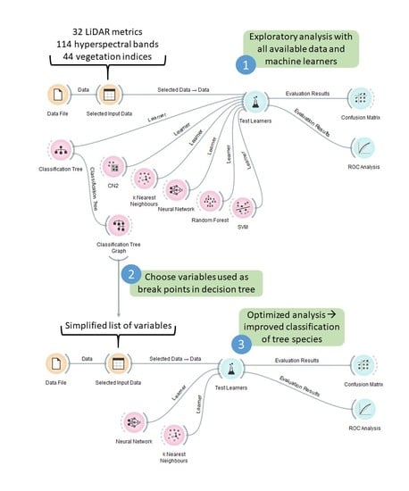
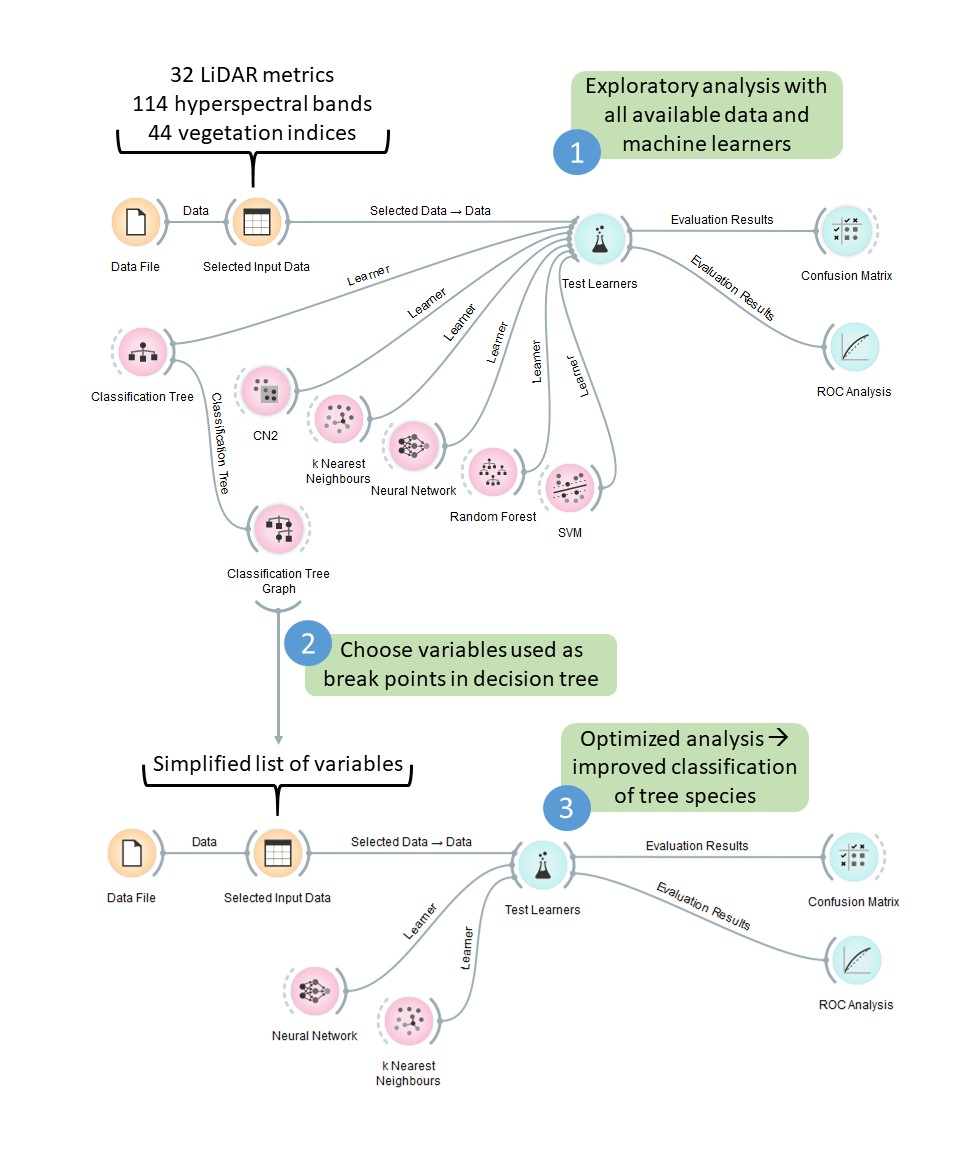
Numerous methods for machine learning are available, spanning a wide range of data analysis techniques. Overall, the methods used here can be broken down into classification tree methods (decision trees, random forest), methods based on grouping and separability (support vector machines (SVM), k-nearest neighbors), and methods based on rule creation and application (CN2 rules, naïve Bayes, neural networks). The Orange Data Mining Extension for Python, version 2.7 [61] was used to test each of the above classification methods (Figure 1a). Classifier performance was assessed by calculating overall classification accuracy (CA), area under the curve of the receiving operator characteristic (AUC-ROC) [86], Brier scores [87], and Cohen’s kappa coefficient [88,89] for each combination. Orange automatically generates and reports AUC-ROC values and Brier scores when machine learning classifiers are run, as well as a confusion matrix and classification accuracy value. Custom Python code was written to calculate the kappa coefficient from the confusion matrix.
As a baseline for comparison to the explanatory power of simplified datasets, all machine learners described above were tested on full datasets consisting of 32 LiDAR metrics, 114 hyperspectral bands, 44 vegetation indices, or all 190 variables. After testing, the two best-performing machine learners, as determined by highest classification accuracy, AUC-ROC, Brier score, and kappa coefficient, were selected for use in further analyses. In all cases, classification accuracies were determined by applying each trained machine learner to subsets of input data with known dominant species identity. Specifically, cross-validation resampling, in which data on each dominant species serve as training data in one of multiple rounds of machine learning by each classifier, was used to generate confusion matrices from which each overall classification accuracy was calculated.
For use in combination with the two best machine learning techniques, the list of input variables was also reduced to a simplified list, optimized to include the most informative variables available for each forest. The classification tree run on each dataset during the initial exploratory analysis was examined using the Tree Viewer widget in Orange. These trees were used to construct lists of variables that represent informative breaks in the dataset. LiDAR metrics, vegetation indices, or reflectance bands found in the first five levels of classification tree nodes were compiled to create simplified lists. Lists were also made from the first ten levels of classification tree nodes, but these longer lists were found to be no more informative than those from the first five levels; thus, they are not discussed in the results section.
Variables identified from classification tree breaks were then used to construct five simplified lists of input data per forest. The classification tree run on the reflectance bands alone was used to construct a simplified list of select reflectance bands. Lists were constructed in the same way from classification trees run on the full list of vegetation indices to create a simplified vegetation indices list and on the entire dataset of 190 LiDAR and hyperspectral variables to create a simplified list containing variables of all data types. In the case of the LiDAR metrics, lists were made for individual forests, and a common list of metrics shared across forests was also made in an attempt to identify some generalizable aspects of LiDAR data that may have strong explanatory power in other forests (Table 4). Using only these simplified lists of metrics as inputs, the two best classification and resampling methods as determined above were rerun and reassessed on the basis of CA, AUC-ROC, Brier score, and kappa coefficient (Figure 1b).
In order to compare this method of dimensionality reduction to an established statistical technique, principal component analysis (PCA) was also performed on a dataset constructed from a raster stack of all hyperspectral reflectance bands, using the Forward PC Rotation function in ENVI Classic. PCA was performed on this dataset only because of missing values in LiDAR metric rasters and because of the difficulty of interpretation of principle components created from all vegetation indices, in which mathematical transformations were already applied to reflectance data. The resulting principal components with eigenvalues greater than one (10 principal components for each forest) were exported as raster files and used as inputs to machine learning classifiers as described above for other datasets.
3. Results
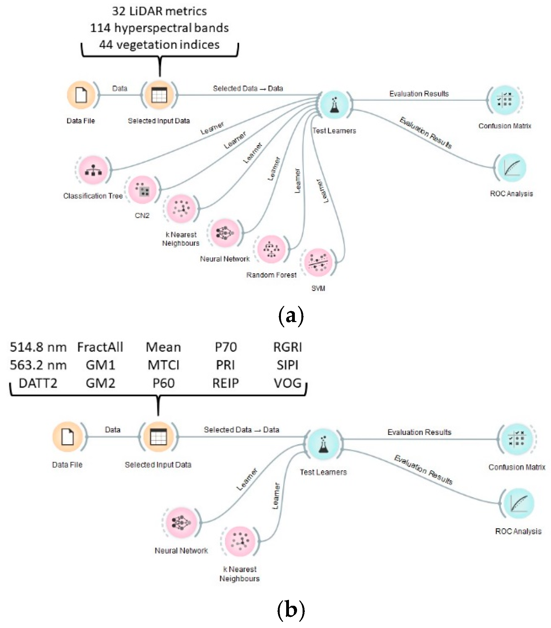
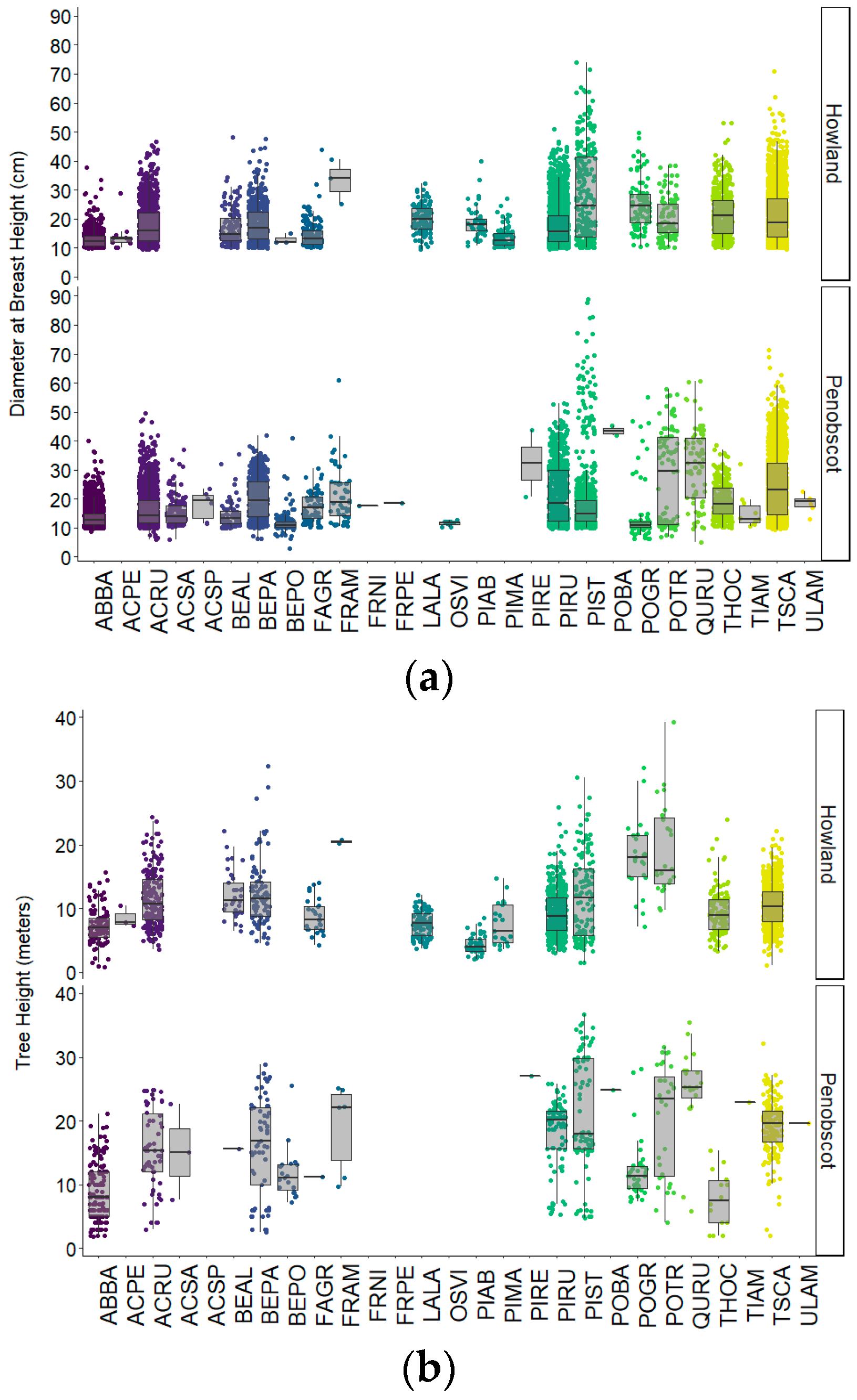
An initial assessment of species-specific structure shows that individual tree DBH and height measurements in Howland and Penobscot Experimental Forests vary in absolute magnitude and in degree of within-species variability (Figure 2). This variability is unsurprising given that these biometry data are also comparing across tree ages and growing conditions. Nonetheless, interspecies variability in these parameters illustrates key characteristics of tree community composition at each forest site.
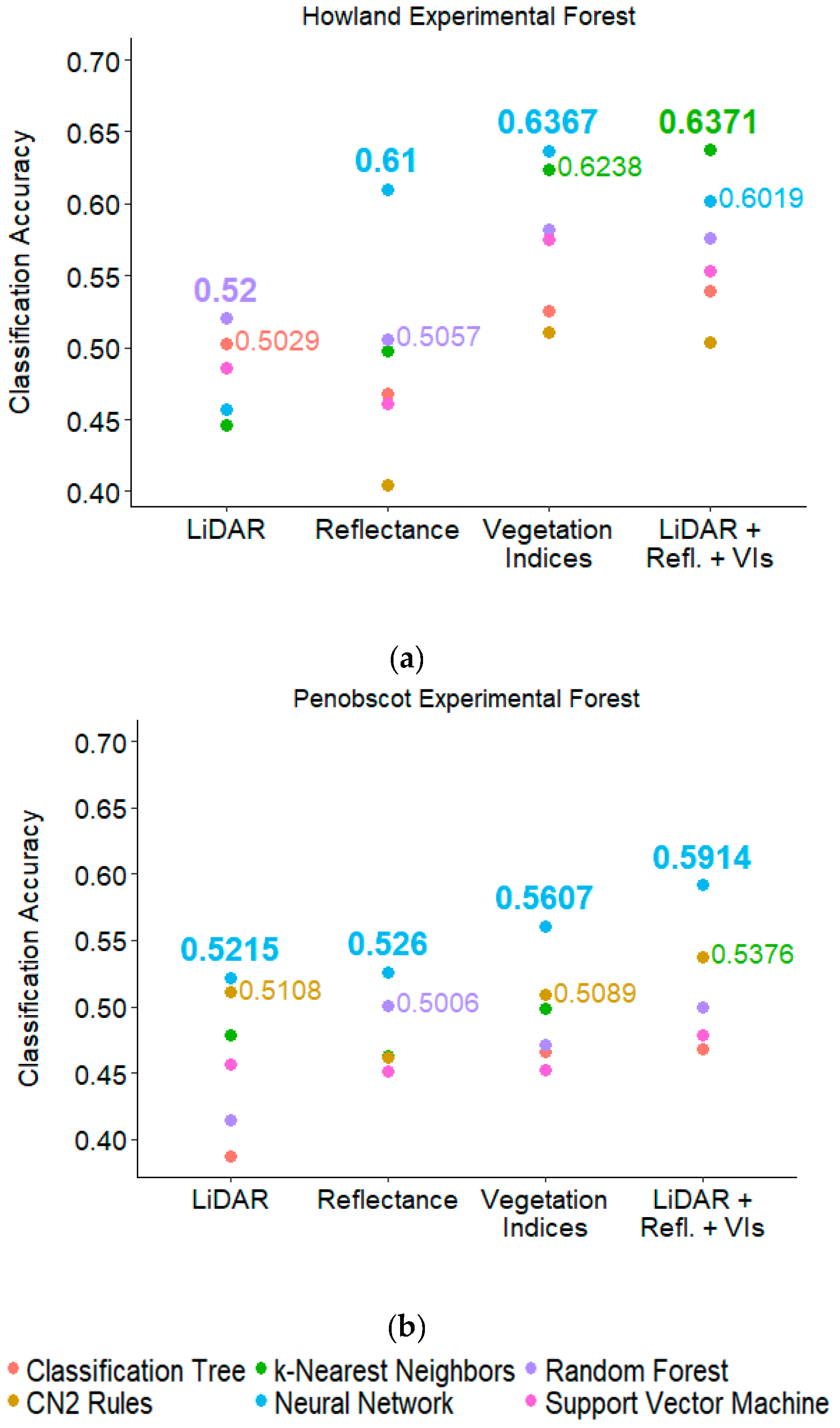
Results of our initial exploratory analysis show that, in both forests, use of the full dataset containing both spectral and structural data resulted in higher classification accuracies, 0.6371 for Howland Experimental Forest and 0.5914 for Penobscot Experimental Forest, than using any of the three individual data types alone (Figure 3). Across forests, using LiDAR data alone resulted in slightly lower classification accuracies than either type of hyperspectral data, and the use of vegetation indices as machine learning inputs resulted in higher accuracies than using raw reflectance data. Indeed, classification accuracies achieved using vegetation indices were nearly equal to that from the full hyperspectral and LiDAR dataset in Howland Experimental Forest (CA = 0.6367) (Figure 3). Although the performance of individual machine learning techniques varied by data type and forest, k-nearest neighbors, random forest, and neural network classifiers tended to outperform other options. In both forests, all machine learning techniques produced higher accuracies when run with cross-validation resampling; only these results are shown in Figure 3 and Figure 4. Finally, classification accuracies from data on Howland Experimental Forest (maximum CA = 0.6371) were higher across the board than those from Penobscot Experimental Forest (maximum CA = 0.5914).
Table 4 shows the simplified lists of inputs used for the second round of machine learning analysis. Dimensionality is greatly reduced as compared to the full dataset; this is particularly evident in the case of the hyperspectral reflectance bands, where only 13 bands (Howland Experimental Forest) or 16 bands (Penobscot Experimental Forest) were retained, representing an approximately 90% reduction in the number of input variables. In the case of the reflectance only dataset, selected bands covered the full range of available wavelengths. A wide range of vegetation indices optimized for chlorophylls, cartenoids, anthocyanins, and xanthophylls were also identified as important variables for interspecies distinction. The LiDAR metrics identified by this method include both FCover, a general measure of forest density and extent, and Fract_All, which quantifies the relative number of multiple LiDAR collisions with vegetation due to within-canopy structure, and height percentile and density decile parameters that provide detailed information on vertical distribution of canopy elements. Five paramters, D9, FCover, FractAll, P50, and P100, were selected in both forests, suggesting that this methodology can be used to identify key structural characteristics of species, as well as pigment-related reflectance differences.
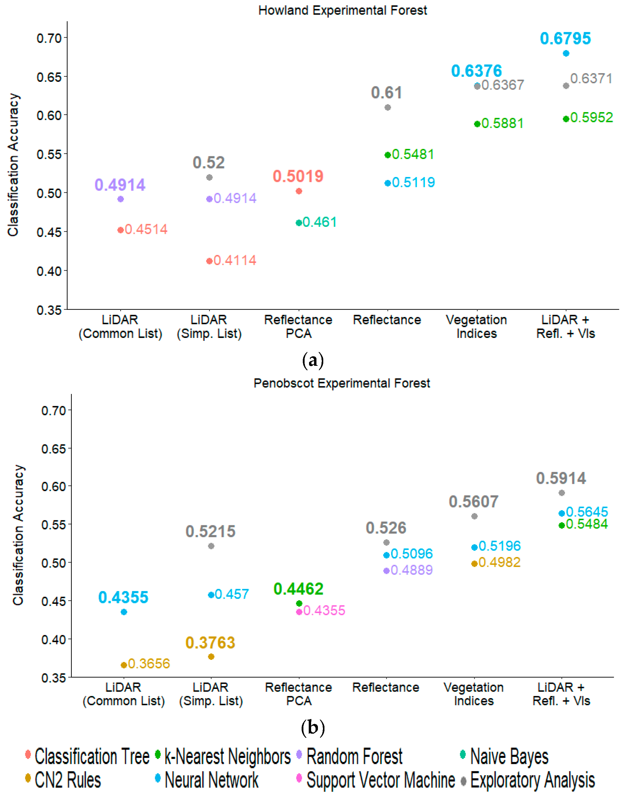
The use of the combined list of hyperspectral and LiDAR inputs yielded higher classification accuracies (Figure 4) and kappa coefficients (Figure 5) than any individual dataset alone, demonstrating that LiDAR and hyperspectral datasets contain complementary information. When comparing between the performance of machine learners run with inputs from individual datasets, use of the simplified lists of vegetation indices also resulted in high classification accuracies. Machine learners trained on a simplified list of reflectance bands outperformed those trained on the principal components created from the reflectance dataset, demonstrating that dimensionality can be reduced with our methodology while retaining superior separability among species. In Figure 4, the greatest classification accuracies from the exploratory analysis are overlaid in gray on results from analyses on the simplified lists. Although all six available machine learning techniques were tried on these PCA datasets as in the exploratory analysis step, results from only the two with the highest classification accuracy or kappa coefficient results are shown in Figure 4 and Figure 5 for ease of comparison. For Howland Experimental Forest, classification accuracies improved or remained comparable to those achieved using the full dataset, even with the significant dimensionality reduction performed here. In data from Penobscot Experimental Forest, simplified lists were slightly outperformed by runs using the full dataset in all cases. Nevertheless, the similar or, in some cases, improved performance of machine learners run on a significantly smaller dataset implies that our selection methodology is able to produce a list of inputs optimized for high separability among tree species.
4. Discussion
Results from combined LiDAR, vegetation index, and hyperspectral reflectance datasets across forests suggest that the combination of spectral and structural information is richer in detail than any individual dataset alone. This improvement is in line with other studies that found a similar effect [20,90]. The fact that the incorporation of LiDAR data improved the hyperspectral-based classifications of tree species, particularly at Howland Experimental Forest, speaks to the utility of machine learning techniques in solving problems like this one. Some researchers previously postulated that LiDAR datasets do not suffer as much from the issues of ill-posed problems and very high dimensionality and are, therefore, better suited to classification techniques that would not necessarily be optimal for other remote-sensing work [91]. This, along with our dimensionality reduction methodology, may account for some of the differences between the results described here and other previously published studies that did not find improvements in classification accuracy when adding LiDAR data to hyperspectral datasets [39,92].
Nonetheless, there remain some limitations to the analysis as presented here. Firstly, the inclusion of LiDAR metrics, such as the mean and standard deviation rasters, which are necessarily specific to the tree heights in the forest on which they were calculated, may limit the generalizability of this analysis. Secondly, this analysis necessitated use of aggregated data. While this is not a constraint that will necessarily apply to all future studies, aggregation of data to a subplot level was required in this case because of the lack of data on the coordinates of individual trees within either forest. The aggregation of this biometry data by subplot-level stem count is just one of several ways in which data could have been meaningfully summarized [93]. Although initial exploration of aggregation methods revealed that the majority of subplots would be assigned the same dominant species regardless of method, this choice necessarily affects the exact classification accuracies achieved in this analysis. Additionally, any aggregation means that some detail is necessarily lost, particularly from the field campaign dataset, which provided data on height and DBH at an individual tree level, and from the hyperspectral datasets. Within each subplot, several hundred 1-m2 pixels were averaged together during the aggregation process, meaning that a great deal of detail on differential reflectance from within individual tree crowns could not be used.
This is a problem that was confronted by numerous researchers in the past, since G-LiHT is certainly not the only dataset to include data aggregated to different sizes or to rely on ground-truth data with some limitations. Some authors argued that attempts to identify or classify species at anything above the individual tree level will be met with difficulty [24], but other researchers previously published classifications with up to 90% on tree stands [94]. In the case of the datasets used here, aggregation to a mean subplot value necessarily creates some error due to loss of detail and because of the contaminating effect of non-dominant species’ spectral signatures, as well as any visible shrub understory or bare ground, for which it was impossible to fully account in this classification. Nonetheless, a classification accuracy of over 67% demonstrates again that such datasets can still be used to generate reliable results, an encouraging result given that previous researchers reported stand effects that explain a similar amount of variance in LiDAR returns, as with species identity [25].
Although the combination of spectral and structural data in this and future analyses will likely always necessitate data aggregation or spatial mismatch, our analysis shows that the benefits of dataset fusion outweigh the costs. Both simplified lists of inputs combining data from all three data types include an intriguing mix of variables. Across forests, these simplified lists contain numerous variables related to leaf greenness and pigment concentrations. All hyperspectral reflectance bands selected for the simplified list containing all data types fall between 500 and 600 nm, the green portion of the spectrum. Similarly, the majority of vegetation indices included in the simplified lists were related to anthocyanin, carotenoid, and chlorophyll concentrations, either directly or as a measure of the red edge of the vegetation reflectance spectrum. As a complement, the LiDAR metrics included in these lists include parameters representing broad structural features within forest canopies, including the P50 and P100 parameters widely used to quantify forest biomass and height in LiDAR inventory studies [95], as well as the Fract_All and density parameters that provide insight into crown and canopy structure. The consistent selection of these parameters across sites indicates that the methodology used here is capable of identifying characteristics of vegetation that are both fundamentally important and useful in distinguishing between tree species within a single region of forest canopy.
The selection of particular machine learners over others is also a key factor in determining the success of tree species classifications. In this analysis, neural networks, k-nearest neighbors, and random forest methods generally outperformed the others available through Orange. Historically, support vector machines were used with success on remotely sensed datasets, including in other recent attempts at tree species classification [37]. This is likely due to the fact that support vector machines (SVM) are designed to handle datasets of very high dimensionality, making them the established standard for hyperspectral remote-sensing work [96]. However, on our datasets with reduced dimensionality, the strengths of other machine learning techniques may have led to their superior performance. Early work on the use of neural networks highlighted their suitability for multisource datasets [97], and the entire neural network principle is based on the capacity of each neuron in the network to shift and change as the network handles more or new data [98]. Similarly, the CN2 rules algorithm was invented to create rules that can be applied to data points that fit well, but imperfectly, with known classes, rather than excluding all imperfect matches [99]. The benefit of such flexibility is easily seen when considering the variability in growth form and leaf reflectance from individuals of the same species in a forest, although this analysis by no means confirms this as the precise reason for the high performance of these machine learning techniques in this analysis. Further work should explore within-species variability as an important factor in machine learning work for tree species classification on the landscape scale.
5. Conclusions
In this analysis, neural networks, k-nearest neighbors, and random forest methods were used to achieve high classification accuracies when distinguishing among tree species using simplified and optimized lists of hyperspectral and LiDAR variables. This analysis supports a growing body of knowledge on the utility of datasets containing complementary structural and spectral information. Given the potential for land-cover classification using LiDAR data on land surface properties [100], such fused datasets may better reveal the structure and shadowing effects of canopy gaps or other irregularities that would otherwise hinder species classifications using spectral data alone. It was shown that using data on aboveground biomass in conjunction with structural information on forest structure generated by the laser vegetation imaging sensor (LVIS) improves the ability of models to predict the size of forest carbon stocks [21]. It now seems that the combination of these two data types may be able to simultaneously help identify tree species, thereby opening up the possibility of generating species-specific carbon estimates with a similar combined dataset. Other researchers looking to the future of remote sensing also highlighted the utility of LiDAR data in addressing large-scale questions like deforestation and carbon sequestration in whole forests on a species-specific basis [1,31].
When looking to the future of multi-sensoral and fused datasets, one of the commonly cited challenges is the development or discovery of analytical methods that can properly integrate data collected by different sensors or by different projects altogether. While variable reduction techniques used here showed mixed results depending on the exact set of inputs to each machine learner, it appears that dimensionality reduction based on classification tree nodes is a technique worth trying on fused or multisource remote sensing datasets. In summary, the capability of data mining and machine learning interfaces like Orange to optimize classification workflows is clearly powerful. Further work should be done to optimize the production of simplified datasets combining information from a variety of sensors in order to better understand, monitor, and quantify heterogeneously distributed tree species.
Author Contributions
Conceptualization, J.M. and W.N-M.; methodology, J.M. and W.N-M.; software, J.M.; validation, J.M.; formal analysis, J.M.; investigation, J.M. and W.N-M.; resources, W.N-M.; data curation, J.M.; writing—original draft preparation, J.M.; writing—review and editing, W.N-M.; visualization, J.M.; supervision, W.N-M.; project administration, W.N-M; funding acquisition, J.M. and W.N-M.
Funding
This research was funded in part by a grant from the Society of Woman Geographers.
Acknowledgments
We would like to thank Bruce Cook for data processing and valuable discussion in the development of this manuscript.
Conflicts of Interest
The authors declare no conflict of interest. The funders had no role in the design of the study; in the collection, analyses, or interpretation of data; in the writing of the manuscript, or in the decision to publish the results.
References
- Koch, B. Status and future of laser scanning, synthetic aperture radar and hyperspectral remote sensing data for forest biomass assessment. ISPRS J. Photogramm. Remote Sens. 2010, 65, 581–590. [Google Scholar] [CrossRef]
- Korhonen, L.; Korpela, I.; Heiskanen, J.; Maltamo, M. Airborne discrete-return LIDAR data in the estimation of vertical canopy cover, angular canopy closure and leaf area index. Remote Sens. Environ. 2011, 115, 1065–1080. [Google Scholar] [CrossRef]
- Schardt, M.; Ziegler, M.; Wimmer, A.; Wack, R.; Hyyppä, J. Assessment of forest parameters by means of laser scanning. In Proceedings of the International Archives of Photogrammetry Remote Sensing and Spatial Information Sciences, Graz, Austria, 9–13 September 2002; pp. 302–309. [Google Scholar]
- Wulder, M.A.; Bater, C.W.; Coops, N.C.; Hilker, T.; White, J.C. The role of LiDAR in sustainable forest management. For. Chron. 2008, 84, 807–826. [Google Scholar] [CrossRef] [Green Version]
- Reitberger, J.; Krzystek, P.; Stilla, U. Analysis of full waveform LIDAR data for the classification of deciduous and coniferous trees. Int. J. Remote Sens. 2008, 29, 1407–1431. [Google Scholar] [CrossRef]
- Zhou, T.; Popescu, S.C.; Lawing, A.M.; Eriksson, M.; Strimbu, B.M.; Bürkner, P.C. Bayesian and classical machine learning methods: A Comparison for tree species classification with LiDAR waveform signatures. Remote Sens. 2018, 10, 39. [Google Scholar] [CrossRef]
- Heinzel, J.; Koch, B. Exploring full-waveform LiDAR parameters for tree species classification. Int. J. Appl. Earth Obs. Geoinf. 2011, 13, 152–160. [Google Scholar] [CrossRef]
- Cao, L.; Dai, J.; Innes, J.L.; She, G.; Coops, N.C.; Ruan, H. Tree species classification in subtropical forests using small-footprint full-waveform LiDAR data. Int. J. Appl. Earth Obs. Geoinf. 2016, 49, 39–51. [Google Scholar] [CrossRef]
- Lim, K.S.-W.; Treitz, P.; Wulder, M.; St-Onge, B.; Flood, M. Lidar remote sensing of forest structure. Prog. Phys. Geogr. 2003, 27, 88–106. [Google Scholar] [CrossRef]
- Yao, W.; Krzystek, P.; Heurich, M. Tree species classification and estimation of stem volume and DBH based on single tree extraction by exploiting airborne full-waveform LiDAR data. Remote Sens. Environ. 2012, 123, 368–380. [Google Scholar]
- Sumnall, M.J.; Hill, R.A.; Hinsley, S.A. Comparison of small-footprint discrete return and full waveform airborne lidar data for estimating multiple forest variables. Remote Sens. Environ. 2016, 173, 214–223. [Google Scholar] [CrossRef] [Green Version]
- Hudak, A.T.; Evans, J.S.; Smith, A.M.S. LiDAR utility for natural resource managers. Remote Sens. 2009, 1, 934–951. [Google Scholar] [CrossRef]
- Parkes, B.D.; Newell, G.; Cheal, D. Assessing the quality of native vegetation: The “habitat hectares” approach. Ecol. Manag. Restor. 2003, 4, 29–38. [Google Scholar] [CrossRef]
- Laurin, G.V.; Puletti, N.; Chen, Q.; Corona, P.; Papale, D.; Valentini, R. Above ground biomass and tree species richness estimation with airborne lidar in tropical Ghana forests. Int. J. Appl. Earth Obs. Geoinf. 2016, 52, 371–379. [Google Scholar] [CrossRef]
- Fedrigo, M.; Newnham, G.J.; Coops, N.C.; Culvenor, D.S.; Bolton, D.K.; Nitschke, C.R. Predicting temperate forest stand types using only structural profiles from discrete return airborne lidar. ISPRS J. Photogramm. Remote Sens. 2018, 136, 106–119. [Google Scholar] [CrossRef]
- Korpela, I.; Tokola, T.; Orka, H.O.; Koskinen, M. Small-Footprint Discrete-Return Lidar in Tree Species Recognition. In Proceedings of the ISPRS Hannover Workshop 2009, Hannover, Germany, 2–5 June 2009; pp. 1–6. [Google Scholar]
- Van Aardt, J.A.N.; Wynne, R.H.; Scrivani, J.A. Lidar-based Mapping of Forest Volume and Biomass by Taxonomic Group Using Structurally Homogenous Segments. Photogramm. Eng. Remote Sens. 2008, 74, 1033–1044. [Google Scholar] [CrossRef] [Green Version]
- Orka, H.O.; Naesset, E.; Bollandsas, O.M. Utilizing Airborne Laser Intensity for Tree Species Classification. In Proceedings of the SPRS Workshop on Laser Scanning 2007 and SilviLaser 2007, Espoo, Finland, 12–14 September 2007; pp. 1–8. [Google Scholar]
- Gillespie, T.W.; Brock, J.; Wright, C.W. Prospects for quantifying structure, floristic composition and species richness of tropical forests. Int. J. Remote Sens. 2004, 25, 707–715. [Google Scholar] [CrossRef]
- Liu, L.; Pang, Y.; Fan, W.; Li, Z.; Zhang, D.; Li, M. Fused airborne LiDAR and hyperspectral data for tree species identification in a natural temperate forest. J. Remote Sens. 2013, 1007, 679–695. [Google Scholar]
- Ni-Meister, W.; Lee, S.; Strahler, A.H.; Woodcock, C.E.; Schaaf, C.; Yao, T.; Ranson, K.J.; Sun, G.; Blair, J.B. Assessing general relationships between aboveground biomass and vegetation structure parameters for improved carbon estimate from lidar remote sensing. J. Geophys. Res. Biogeosci. 2010, 115, 1–12. [Google Scholar] [CrossRef]
- Jones, T.G.; Coops, N.C.; Sharma, T. Assessing the utility of airborne hyperspectral and LiDAR data for species distribution mapping in the coastal Pacific Northwest, Canada. Remote Sens. Environ. 2010, 114, 2841–2852. [Google Scholar] [CrossRef]
- Alonzo, M.; Bookhagen, B.; Roberts, D.A. Urban tree species mapping using hyperspectral and lidar data fusion. Remote Sens. Environ. 2014, 148, 70–83. [Google Scholar] [CrossRef]
- Yu, X.; Hyyppä, J.; Holopainen, M.; Vastaranta, M. Comparison of area-based and individual tree-based methods for predicting plot-level forest attributes. Remote Sens. 2010, 2, 1481–1495. [Google Scholar] [CrossRef]
- Hovi, A.; Korhonen, L.; Vauhkonen, J.; Korpela, I. LiDAR waveform features for tree species classification and their sensitivity to tree- and acquisition related parameters. Remote Sens. Environ. 2016, 173, 224–237. [Google Scholar] [CrossRef]
- Ferraz, A.; Saatchi, S.; Mallet, C.; Meyer, V. Lidar detection of individual tree size in tropical forests. Remote Sens. Environ. 2016, 183, 318–333. [Google Scholar] [CrossRef]
- Jeronimo, S.M.A.; Kane, V.R.; Churchill, D.J.; McGaughey, R.J.; Franklin, J.F. Applying LiDAR individual tree detection to management of structurally diverse forest landscapes. J. For. 2018, 116, 336–346. [Google Scholar] [CrossRef]
- Zhen, Z.; Quackenbush, L.J.; Zhang, L. Trends in automatic individual tree crown detection and delineation—Evolution of LiDAR data. Remote Sens. 2016, 8, 333. [Google Scholar] [CrossRef]
- Holmgren, J.; Persson, Å.; Söderman, U. Species identification of individual trees by combining high resolution LiDAR data with multi-spectral images. Int. J. Remote Sens. 2008, 29, 1537–1552. [Google Scholar] [CrossRef]
- Cho, M.A.; Mathieu, R.; Asner, G.P.; Naidoo, L.; van Aardt, J.; Ramoelo, A.; Debba, P.; Wessels, K.; Main, R.; Smit, I.P.J.; et al. Mapping tree species composition in South African savannas using an integrated airborne spectral and LiDAR system. Remote Sens. Environ. 2012, 125, 214–226. [Google Scholar] [CrossRef]
- Karna, Y.K.; Hussin, Y.A.; Gilani, H.; Bronsveld, M.C.; Murthy, M.S.R.; Qamer, F.M.; Karky, B.S.; Bhattarai, T.; Aigong, X.; Baniya, C.B. Integration of WorldView-2 and airborne LiDAR data for tree species level carbon stock mapping in Kayar Khola watershed, Nepal. Int. J. Appl. Earth Obs. Geoinf. 2015, 38, 280–291. [Google Scholar] [CrossRef]
- Van Ewijk, K.Y.; Randin, C.F.; Treitz, P.M.; Scott, N.A. Predicting fine-scale tree species abundance patterns using biotic variables derived from LiDAR and high spatial resolution imagery. Remote Sens. Environ. 2014, 150, 120–131. [Google Scholar] [CrossRef]
- Blackburn, G.A. Hyperspectral remote sensing of plant pigments. J. Exp. Bot. 2007, 58, 855–867. [Google Scholar] [CrossRef]
- Kukkonen, M.; Maltamo, M.; Korhonen, L.; Packalen, P. Multispectral Airborne LiDAR Data in the Prediction of Boreal Tree Species Composition. IEEE Trans. Geosci. Remote Sens. 2019, 1–10. [Google Scholar] [CrossRef]
- Budei, B.C.; St-Onge, B.; Hopkinson, C.; Audet, F.A. Identifying the genus or species of individual trees using a three-wavelength airborne lidar system. Remote Sens. Environ. 2018, 204, 632–647. [Google Scholar] [CrossRef]
- Amiri, N.; Heurich, M.; Krzystek, P.; Skidmore, A.K. Feature relevance assessment of multispectral airborne LiDAR data for tree species classification. Int. Arch. Photogramm. Remote Sens. Spat. Inf. Sci.-ISPRS Arch. 2018, 42, 31–34. [Google Scholar] [CrossRef]
- Wessel, M.; Brandmeier, M.; Tiede, D. Evaluation of different machine learning algorithms for scalable classification of tree types and tree species based on Sentinel-2 data. Remote Sens. 2018, 10, 1419. [Google Scholar] [CrossRef]
- Blackburn, G.A. Remote sensing of forest pigments using airborne imaging spectrometer and LIDAR imagery. Remote Sens. Environ. 2002, 82, 311–321. [Google Scholar] [CrossRef]
- Dalponte, M.; Bruzzone, L.; Gianelle, D. Tree species classification in the Southern Alps based on the fusion of very high geometrical resolution multispectral/hyperspectral images and LiDAR data. Remote Sens. Environ. 2012, 123, 258–270. [Google Scholar] [CrossRef]
- Liu, L.; Coops, N.C.; Aven, N.W.; Pang, Y. Mapping urban tree species using integrated airborne hyperspectral and LiDAR remote sensing data. Remote Sens. Environ. 2017, 200, 170–182. [Google Scholar] [CrossRef]
- Swatantran, A.; Dubayah, R.; Roberts, D.; Hofton, M.; Blair, J.B. Mapping biomass and stress in the Sierra Nevada using lidar and hyperspectral data fusion. Remote Sens. Environ. 2011, 115, 2917–2930. [Google Scholar] [CrossRef] [Green Version]
- Andrew, M.E.; Ustin, S.L. Habitat suitability modelling of an invasive plant with advanced remote sensing data. Divers. Distrib. 2009, 15, 627–640. [Google Scholar] [CrossRef]
- Koetz, B.; Morsdorf, F.; van der Linden, S.; Curt, T.; Allgöwer, B. Multi-source land cover classification for forest fire management based on imaging spectrometry and LiDAR data. For. Ecol. Manag. 2008, 256, 263–271. [Google Scholar] [CrossRef]
- Mundt, J.T.; Streutker, D.R.; Glenn, N.F. Mapping sagebrush distribution using fusion of hyperspectral and lidar classifications. Photogramm. Eng. Remote Sens. 2006, 72, 47–54. [Google Scholar] [CrossRef]
- Cook, B.D.; Corp, L.A.; Nelson, R.F.; Middleton, E.M.; Morton, D.C.; McCorkel, J.T.; Masek, J.G.; Ranson, K.J.; Ly, V.; Montesano, P.M. NASA Goddard’s LiDAR, hyperspectral and thermal (G-LiHT) airborne imager. Remote Sens. 2013, 5, 4045–4066. [Google Scholar] [CrossRef]
- Morsdorf, F.; Mårell, A.; Koetz, B.; Cassagne, N.; Pimont, F.; Rigolot, E.; Allgöwer, B. Discrimination of vegetation strata in a multi-layered Mediterranean forest ecosystem using height and intensity information derived from airborne laser scanning. Remote Sens. Environ. 2010, 114, 1403–1415. [Google Scholar] [CrossRef] [Green Version]
- Dalponte, M.; Bruzzone, L.; Vescovo, L.; Gianelle, D. The role of spectral resolution and classifier complexity in the analysis of hyperspectral images of forest areas. Remote Sens. Environ. 2009, 113, 2345–2355. [Google Scholar] [CrossRef]
- Franklin, J. Mapping Species Distributions: Spatial Inference and Prediction; Usher, M., Saunders, D., Peet, R., Dobson, A., Eds.; Cambridge University Press: Cambridge, UK, 2009; ISBN 9780521700023. [Google Scholar]
- Holmgren, J.; Persson, Å. Identifying species of individual trees using airborne laser scanner. Remote Sens. Environ. 2004, 90, 415–423. [Google Scholar] [CrossRef]
- Naesset, E. Airborne laser scanning as a method in operational forest inventory: Status of accuracy assessments accomplished in Scandinavia. Scand. J. For. Res. 2007, 22, 433–442. [Google Scholar] [CrossRef]
- Vauhkonen, J.; Korpela, I.; Maltamo, M.; Tokola, T. Imputation of single-tree attributes using airborne laser scanning-based height, intensity, and alpha shape metrics. Remote Sens. Environ. 2010, 114, 1263–1276. [Google Scholar] [CrossRef]
- Kim, S.; Hinckley, T.; Briggs, D. Classifying individual tree genera using stepwise cluster analysis based on height and intensity metrics derived from airborne laser scanner data. Remote Sens. Environ. 2011, 115, 3329–3342. [Google Scholar] [CrossRef]
- Kavzoglu, T.; Mather, P.M. The role of feature selection in artificial neural network applications. Int. J. Remote Sens. 2002, 23, 2919–2937. [Google Scholar] [CrossRef]
- Murtaugh, P.A. Performance of several variable-selection methods applied to real ecological data. Ecol. Lett. 2009, 12, 1061–1068. [Google Scholar] [CrossRef] [PubMed]
- Kulasekera, K.B. Variable selection by stepwise slicing in nonparametric regression. Stat. Probab. Lett. 2001, 51, 327–336. [Google Scholar] [CrossRef]
- Zou, H.; Hastie, T. Regression and variable selection via the elastic net. J. R. Stat. Soc. Ser. B (Stat. Methodol.) 2005, 67, 301–320. [Google Scholar] [CrossRef]
- Popescu, S.; Mallick, B.; Valle, D.; Zhao, K.; Zhang, X. Hyperspectral remote sensing of plant biochemistry using Bayesian model averaging with variable and band selection. Remote Sens. Environ. 2013, 132, 102–119. [Google Scholar]
- Packalén, P.; Temesgen, H.; Maltamo, M. Variable selection strategies for nearest neighbor imputation methods used in remote sensing based forest inventory. Can. J. Remote Sens. 2012, 38, 557–569. [Google Scholar] [CrossRef]
- Rakotomamonjy, A. Variable Selection Using SVM-based Criteria. J. Mach. Learn. Res. 2003, 3, 1357–1370. [Google Scholar]
- Genuer, R.; Poggi, J.M.; Tuleau-Malot, C. Variable selection using random forests. Pattern Recognit. Lett. 2010, 31, 2225–2236. [Google Scholar] [CrossRef] [Green Version]
- Demsar, J.; Curk, T.; Erjavec, A.; Gorup, C.; Hocevar, T.; Milutinovic, M.; Mozina, M.; Polajnar, M.; Toplak, M.; Staric, A.; et al. Orange: Data Mining Toolbox in Python. J. Mach. Learn. Res. 2013, 14, 2349–2353. [Google Scholar]
- Montesano, P.M.; Cook, B.D.; Sun, G.; Simard, M.; Nelson, R.F.; Ranson, K.J.; Zhang, Z.; Luthcke, S. Achieving accuracy requirements for forest biomass mapping: A spaceborne data fusion method for estimating forest biomass and LiDAR sampling error. Remote Sens. Environ. 2013, 130, 153–170. [Google Scholar] [CrossRef]
- Evans, J.S.; Hudak, A.T.; Faux, R.; Smith, A.M.S. Discrete return lidar in natural resources: Recommendations for project planning, data processing, and deliverables. Remote Sens. 2009, 1, 776–794. [Google Scholar] [CrossRef]
- Duncanson, L.I.; Dubayah, R.O.; Cook, B.D.; Rosette, J.; Parker, G. The importance of spatial detail: Assessing the utility of individual crown information and scaling approaches for lidar-based biomass density estimation. Remote Sens. Environ. 2015, 168, 102–112. [Google Scholar] [CrossRef]
- Gitelson, A.A.; Merzlyak, M.N. Remote estimation of chlorophyll content in higher plant leaves. Int. J. Remote Sens. 1997, 18, 2691–2697. [Google Scholar] [CrossRef]
- Gitelson, A.A.; Zur, Y.; Chivkunova, O.B.; Merzlyak, M.N. Assessing Carotenoid Content in Plant Leaves with Reflectance Spectroscopy. Photochem. Photobiol. 2002, 75, 272–281. [Google Scholar] [CrossRef]
- Datt, B. Visible/near infrared reflectance and chlorophyll content in eucalyptus leaves. Int. J. Remote Sens. 1999, 20, 2741–2759. [Google Scholar] [CrossRef]
- Tucker, C.J. Red and Photographic Infrared Linear Combinations for Monitoring Vegetation; NASA: Greenbelt, MD, USA, 1979.
- Zarco-Tejada, P.J.; Berjón, A.; López-Lozano, R.; Miller, J.R.; Martín, P.; Cachorro, V.; González, M.R.; De Frutos, A. Assessing vineyard condition with hyperspectral indices: Leaf and canopy reflectance simulation in a row-structured discontinuous canopy. Remote Sens. Environ. 2005, 99, 271–287. [Google Scholar] [CrossRef]
- Maccioni, A.; Agati, G.; Mazzinghi, P. New vegetation indices for remote measurement of chlorophylls based on leaf directional reflectance spectra. J. Photochem. Photobiol. B Biol. 2001, 61, 52–61. [Google Scholar] [CrossRef]
- Chen, J.M. Evaluation of Vegetation Indices and a Modified Simple Ratio for Boreal Applications. Can. J. Remote Sens. 1996, 22, 229–242. [Google Scholar] [CrossRef]
- Dash, J.; Curran, P.J. The MERIS terrestrial chlorophyll index. Int. J. Remote Sens. 2004, 25, 5403–5413. [Google Scholar] [CrossRef]
- Haboudane, D.; Miller, J.R.; Pattey, E.; Zarco-Tejada, P.J.; Strachan, I.B. Hyperspectral vegetation indices and novel algorithms for predicting green LAI of crop canopies: Modeling and validation in the context of precision agriculture. Remote Sens. Environ. 2004, 90, 337–352. [Google Scholar] [CrossRef]
- Sims, D.A.; Gamon, J.A. Relationships between leaf pigment content and spectral reflectance across a wide range of species, leaf structures, and developmental stages. Remote Sens. Environ. 2002, 81, 337–354. [Google Scholar] [CrossRef]
- Rouse, J.W.; Haas, R.H.; Schell, J.A.; Deering, D.W.; Harlan, J.C. Monitoring the Vernal Advancements and Retrogradation of Natural Vegetation; Texas A & M University: College Station, TX, USA, 1974. [Google Scholar]
- Barnes, J.D.; Balaguer, L.; Manrique, E.; Elvira, S.; Davison, A.W. A Reappraisal of the use of DMSO for the extraction and determination of chlorophylls a and b in lichens and other plants. Environ. Exp. Bot. 1992, 32, 85–100. [Google Scholar] [CrossRef]
- Gamon, J.A.; Peñuelas, J.; Field, C.B. A Narrow-Waveband Spectral Index That Tracks Diurnal Changes in Photosynthetic Efficiency. Remote Sens. Environ. 1992, 41, 35–44. [Google Scholar] [CrossRef]
- Roujean, J.; Breon, F. Estimating PAR absorbed by vegetation from bidirectional reflectance measurements. Remote Sens. Environ. 1995, 51, 375–384. [Google Scholar] [CrossRef]
- Broge, N.H.; Leblanc, E. Comparing prediction power and stability of broadband and hyperspectral vegetation indices for estimation of green leaf area index and canopy chlorophyll density. Remote Sens. Environ. 2000, 76, 156–172. [Google Scholar] [CrossRef]
- Gamon, J.A.; Surfus, J.S. Assessing leaf pigment content and activity with a reflectometer. New Phytol. 1999, 143, 105–117. [Google Scholar] [CrossRef] [Green Version]
- Penuelas, J.; Baret, F.; Filella, I. Semi-empirical indices to assess carotenoids/chlorophyll a ratio from leaf spectral reflectance. Photosynthetica 1995, 31, 221–230. [Google Scholar]
- Vogelmann, J.E.; Rock, B.N.; Moss, D.M. Red edge spectral measurements from sugar maple leaves. Int. J. Remote Sens. 1993, 14, 1563–1575. [Google Scholar] [CrossRef]
- Northern Research Station Howland Cooperating Experimental Forest. Available online: https://www.nrs.fs.fed.us/ef/locations/me/howland_cef/ (accessed on 12 March 2019).
- Seymour, R.; Crandall, M.; Rogers, N.; Kenefic, L.; Sendak, P. Sixty Years of Silviculture in a Northern Conifer Forest in Maine, USA. For. Sci. 2017, 64, 102–111. [Google Scholar]
- Brissette, J.C.; Kenefic, L.S. History of the Penobscot Experimental Forest, 1950–2010; Forest Service, Northern Research Station: Newtown Square, PA, USA, 2014. [Google Scholar]
- Fawcett, T. An introduction to ROC analysis. Pattern Recognit. Lett. 2006, 27, 861–874. [Google Scholar] [CrossRef]
- Hernandez-Orallo, J.; Flach, P.; Ferri, C. Brier Curves: A New Cost-Based Visualisation of Classifier Performance. In Proceedings of the the 28th International Conference on Machine Learning (ICML-11), Bellevue, WA, USA, 28 June–2 July 2011; pp. 1–27. [Google Scholar]
- Cohen, J. A Coefficient of Agreement for Nominal Scales. Educ. Psychol. Meas. 1960, 20, 37–46. [Google Scholar] [CrossRef]
- Congalton, R.G.; Green, K. Assessing the Accuracy of Remotely Sensed Data: Principles and Practices, 2nd ed.; CRC Press, Taylor and Francis Group: Boca Raton, FL, USA, 2009. [Google Scholar]
- Anderson, J.E.; Plourde, L.C.; Martin, M.E.; Braswell, B.H.; Smith, M.L.; Dubayah, R.O.; Hofton, M.A.; Blair, J.B. Integrating waveform lidar with hyperspectral imagery for inventory of a northern temperate forest. Remote Sens. Environ. 2008, 112, 1856–1870. [Google Scholar] [CrossRef]
- Ducic, V.; Hollaus, M.; Ullrich, A.; Wagner, W.; Melzer, T. 3D Vegetation Mapping And Classification Using Full-Wavevorm Laser Scanning. In Proceedings of the International Workshop 3D Remote Sensing in Forestry, Vienna, Austria, 14–15 February 2006; Volume Session 8a, pp. 211–217. [Google Scholar]
- Ghosh, A.; Fassnacht, F.E.; Joshi, P.K.; Koch, B. A framework for mapping tree species combining hyperspectral and LiDAR data: Role of selected classifiers and sensor across three spatial scales. Int. J. Appl. Earth Obs. Geoinf. 2014, 26, 49–63. [Google Scholar] [CrossRef]
- Guo, Q.; Rundel, P.W. Measuring dominance and diversity in ecological communities: Choosing the right variables. J. Veg. Sci. 1997, 8, 405–408. [Google Scholar] [CrossRef]
- Korpela, I.; Orka, H.O.; Maltamo, M.; Tokola, T.; Hyyppa, J. Tree Species Classification Using Airborne LiDAR-Effects of Stand and Tree Parameters, Downsizing of Training Set, Intensity Normalization, and Sensor Type. Silva Fenn. 2010, 44, 319–339. [Google Scholar] [CrossRef]
- Drake, J.B.; Dubayah, R.O.; Clark, D.B.; Knox, R.G.; Blair, J.B.; Hofton, M.A.; Chazdon, R.L.; Weishampel, J.F.; Prince, S. Estimation of tropical forest structural characteristics, using large-footprint lidar. Remote Sens. Environ. 2002, 79, 305–319. [Google Scholar] [CrossRef]
- Pal, M.; Mather, P.M. Support vector machines for classification in remote sensing. Int. J. Remote Sens. 2005, 26, 1007–1011. [Google Scholar] [CrossRef]
- Benediktsson, J.A.; Swain, P.H.; Erosy, O.K. Methods in Classification of Multisource. IEEE Trans. Geosci. Remote Sens. 1990, 28, 540–552. [Google Scholar]
- Haykin, S. Neural Networks: A Comprehensive Foundation, 2nd ed.; Prentice Hall: Upper Saddle River, NJ, USA, 2004. [Google Scholar]
- Clark, P.; Niblett, T. The CN2 induction algorithm. Mach. Learn. 1989, 3, 261. [Google Scholar] [CrossRef]
- Brennan, R.; Webster, T.L. Object-oriented land cover classification of lidar-derived surfaces. Can. J. Remote Sens. 2006, 32, 162–172. [Google Scholar] [CrossRef]
Figure 1.
Sample Orange workflow for comparing machine learning methods. In the exploratory analysis step (a), all available machine learning methods were used in combination with the full suite of available data. In the simplified analysis (b), only the two best-performing machine learners were used on a simplified list of input variables, one example of which is shown here.

Figure 2.
Plots of individual tree diameters at breast height by species. Summary of diameter at breast height data (a) and individual tree height data (b) for on trees in experimental plots in Howland Experimental Forest and Penobscot Experimental Forest. Dots represent data on individual trees; overlaid box-and-whisker plots summarize distribution of values by species for each forest.

Figure 3.
Comparison of resampling techniques and machine learning methods using complete lists of metrics. Figure shows classification accuracies achieved by machine learners run on full datasets from Howland Experimental Forest (a) and Penobscot Experimental Forest (b). From left to right, columns represent classification accuracies produced with light detection and ranging (LiDAR) data, hyperspectral reflectance data, vegetation indices (VIs) calculated from these reflectance data, and a combined dataset of LiDAR and both types of hyperspectral data.

Figure 4.
Classification accuracies achieved by machine learners run on simplified datasets from Howland Experimental Forest (a) and Penobscot Experimental Forest (b). Dot color represents the machine learning technique used in each case. Gray dots represent classification accuracies achieved during the exploratory analysis step using the full dataset, and are shown as a comparison.

Figure 5.
Kappa coefficients achieved by machine learners run on simplified datasets from Howland Experimental Forest (a) and Penobscot Experimental Forest (b). Dot color represents the machine learning technique used in each case.
Figure 5.
Kappa coefficients achieved by machine learners run on simplified datasets from Howland Experimental Forest (a) and Penobscot Experimental Forest (b). Dot color represents the machine learning technique used in each case.


Table 1.
Full list of light detection and ranging (LiDAR) metrics and abbreviations.
| Name and Description of Metric | Units | Abbreviation |
|---|---|---|
| Mean absolute deviation = mean (|height − mean height|) of tree returns | Meters | AAD |
| Canopy relief ratio = ((mean − min)/(max − min)) of tree returns | Unitless | CRR |
| Density deciles of tree returns (number of returns in 10% height bins/total LiDAR returns) | Fraction | D0–D9 |
| Fraction of first return pulses intercepted by tree | Fraction | FCover |
| Fraction of all returns classified as tree | Fraction | FractAll |
| Interquartile range (P75–P25) of tree returns | Meters | IQR |
| Kurtosis of tree return heights | Meters | Kurt |
| Median absolute deviation = median (|height − median height|) of tree returns | Meters | MAD |
| Mean of tree return heights | Meters | Mean |
| Height percentiles (10% increments) of tree returns | Meters | P10–P100 |
| Quadratic mean of tree return heights | Meters | QMean |
| Skewness of tree return heights | Meters | Skew |
| Standard deviation of tree return heights | Meters | StDev |
| Vertical distribution ratio = (P100 − P50)/P100 | Unitless | VDR |
Table 2.
Select list of hyperspectral vegetation indices and abbreviations used in final analyses.
| Name of Vegetation Index | Abbreviation | Reference |
|---|---|---|
| Anthocyanin reflectance index 1 | ARI1 | [65] |
| Anthocyanin reflectance index 2 | ARI2 | [65] |
| Carotenoid reflectance index 2 | CRI2 | [66] |
| Datt 1 | DATT1 | [67] |
| Datt 2 | DATT2 | [67] |
| Difference vegetation index | DVI | [68] |
| Greenness index | GI | [69] |
| Gitelson and Merzlyak 1 | GM1 | [65] |
| Gitelson and Merzlyak 2 | GM2 | [65] |
| Maccioni | MAC | [70] |
| Modified simple ratio | MSR | [71] |
| Medium Resolution Imaging Spectrometer (MERIS) terrestrial chlorophyll index | MTCI | [72] |
| Modified triangular vegetation index | MTVI | [73] |
| Modified triangular vegetation index 2 | MTVI2 | [73] |
| Modified red edge normalized difference vegetation index | MRENDVI | [74] |
| Normalized difference vegetation index | NDVI | [75] |
| Normalized phaeophytinization index | NPQI | [76] |
| Photochemical reflectance index | PRI | [77] |
| Renormalized difference vegetation index | RDVI | [78] |
| Red edge inflection point | REIP | [79] |
| Red green ratio index | RGRI | [80] |
| Structure insensitive pigment index | SIPI | [81] |
| Vogelmann | VOG | [82] |
Table 3.
Tree species abbreviations. Species dominant in one or more subplots in either forest are denoted with a letter indicating the forest name: H for Howland Experimental Forest and P for Penobscot Experimental Forest. Species not followed by a letter are not the dominant species in any subplot from either forest.
| Abbreviation | Common and Latin Names | Forest Where Dominant |
|---|---|---|
| ABBA | Balsam fir (Abies balsamea) | H, P |
| ACRU | Red maple (Acer rubrum) | H, P |
| ACSA | Silver maple (Acer saccharinum) | P |
| ACSP | Mountain maple (Acer spicatum) | P |
| BEAL | Yellow birch (Betula alleghaniensis) | P |
| BEPA | Paper birch (Betula papyrifera) | P |
| BEPO | Gray birch (Betula populifolia) | P |
| FAGR | American beech (Fagus grandifolia) | H, P |
| FRAM | White ash (Fraxinus americana) | H |
| FRPE | Green ash (Fraxinus pennsylvanica) | |
| LALA | Tamarack (Larix laricina) | |
| OSVI | Eastern hophornbeam (Ostrya virginiana) | |
| PIAB | Norway spruce (Picea abies) | H |
| PIMA | Black spruce (Picea mariana) | H |
| PIRE | Red pine (Pinus resinosa) | P |
| PIRU | Red spruce (Picea rubens) | P |
| PIST | Eastern white pine (Pinus strobus) | H, P |
| POBA | Balsam poplar (Populus balsamifera) | |
| POGR | Bigtooth aspen (Populus grandidentata) | P |
| POTR | Quaking aspen (Populus tremuloides) | P |
| QURU | Northern red oak (Quercus rubra) | |
| TIAM | American basswood (Tilia americana) | |
| THOC | Northern white cedar (Thuja occidentalis) | H, P |
| TSCA | Eastern hemlock (Tsuga canadensis) | H, P |
| ULAM | American elm (Ulmus americana) |
Table 4.
Simplified lists of machine learning inputs. Variables used in nodes within the first five levels of classification trees constructed on the full dataset were added to simplified lists serving as inputs for further machine learning analyses. Metrics used to construct the common list of LiDAR metrics are highlighted in gray to indicate shared status across forests.
| Penobscot Experimental Forest | Howland Experimental Forest | ||||||
|---|---|---|---|---|---|---|---|
| LiDAR Metrics | Refl. Bands | Veg. Indices | LiDAR + Refl. + VIs | LiDAR Metrics | Refl. Bands | Veg. Indices | LiDAR + Refl. + VIs |
| D0 | 426.8 nm | ARI1 | 558.8 nm | D3 | 426.8 nm | ARI1 | 514.8 nm |
| D2 | 484.0 nm | ARI2 | 563.2 nm | D5 | 497.2 nm | ARI2 | 563.2 nm |
| D9 | 545.6 nm | DATT1 | 576.4 nm | D6 | 528.0 nm | CRI2 | DATT2 |
| FCover | 572.0 nm | DVI | 594.0 nm | D9 | 576.4 nm | DATT2 | FractAll |
| FractAll | 580.8 nm | GM1 | ARI2 | FCover | 580.8 nm | GI | GM1 |
| Kurtosis | 602.8 nm | MAC | CRI2 | FractAll | 651.2 nm | GM2 | GM2 |
| Mean | 655.6 nm | MTCI | D4 | P50 | 673.2 nm | PRI | Mean |
| P10 | 660.0 nm | MTVI | D6 | P60 | 686.4 nm | RDVI | MTCI |
| P40 | 673.2 nm | MTVI2 | GM1 | P90 | 690.8 nm | RGRI | P60 |
| P50 | 800.8 nm | MRENDVI | MSR | P100 | 721.6 nm | SIPI | P70 |
| P80 | 888.8 nm | NDVI | MTCI | 730.4 nm | PRI | ||
| P100 | 906.4 nm | NPQI | NPQI | 761.2 nm | REIP | ||
| StDev | 915.2 nm | PRI | P20 | 792.0 nm | RGRI | ||
| REIP | P100 | 862.4 nm | SIPI | ||||
| SIPI | RDVI | 906.4 nm | VOG | ||||
| StDev | 910.8 nm | ||||||
© 2019 by the authors. Licensee MDPI, Basel, Switzerland. This article is an open access article distributed under the terms and conditions of the Creative Commons Attribution (CC BY) license (http://creativecommons.org/licenses/by/4.0/).
Share and Cite
MDPI and ACS Style
Marrs, J.; Ni-Meister, W. Machine Learning Techniques for Tree Species Classification Using Co-Registered LiDAR and Hyperspectral Data. Remote Sens. 2019, 11, 819. https://0-doi-org.brum.beds.ac.uk/10.3390/rs11070819
AMA Style
Marrs J, Ni-Meister W. Machine Learning Techniques for Tree Species Classification Using Co-Registered LiDAR and Hyperspectral Data. Remote Sensing. 2019; 11(7):819. https://0-doi-org.brum.beds.ac.uk/10.3390/rs11070819
Chicago/Turabian StyleMarrs, Julia, and Wenge Ni-Meister. 2019. "Machine Learning Techniques for Tree Species Classification Using Co-Registered LiDAR and Hyperspectral Data" Remote Sensing 11, no. 7: 819. https://0-doi-org.brum.beds.ac.uk/10.3390/rs11070819
Note that from the first issue of 2016, this journal uses article numbers instead of page numbers. See further details here.