Wet and Dry Snow Detection Using Sentinel-1 SAR Data for Mountainous Areas with a Machine Learning Technique

Abstract

Traditional studies on mapping wet snow cover extent (SCE) often feature limitations, especially in vegetated and mountainous areas. The aim of this study is to propose a new total and wet SCE mapping strategy based on freely accessible spaceborne synthetic aperture radar (SAR) data. The approach is transferable on a global scale as well as for different land cover types (including densely vegetated forest and agricultural regions), and is based on the use of backscattering coefficient, interferometric SAR coherence, and polarimetric parameters. Furthermore, four topographical factors were included in the simple tuning of random forest-based land cover type-dependent classification strategy. Results showed the classification accuracy was above 0.75, with an F-measure higher than 0.70, in all five selected regions of interest located around globally distributed mountain ranges. Whilst excluding forest-type land cover classes, the accuracy and F-measure increases to 0.80 and 0.75. In cross-location model set, the accuracy can also be maintained at 0.80 with non-forest accuracy up to 0.85. It has been found that the elevation and polarimetric parameters are the most critical factors, and that the quality of land cover information would also affect the subsequent mapping reliability. In conclusion, through comprehensive validation using optical satellite and in-situ data, our land cover-dependent total SCE mapping approach has been confirmed to be robustly applicable, and the holistic SCE map for different months were eventually derived.

1. Introduction

Snow cover is an important parameter in the context of water availability, the global radiation balance, and natural disasters such as floods and avalanches. It is also a crucial resource for tourism and hydropower generation [1,2,3,4]. Climate change has been affecting snow cover extent (SCE), its amount, and its distribution globally, generally leading to a decline of the aforementioned parameters [5,6,7,8]. This was also stated in the Synthesis Report of Fifth Assessment Report (AR5) of the Intergovernmental Panel on Climate Change (IPCC) [9]. The latest IPCC special report of 2018 reveals severe potential risks due to more extreme SCE changes and melting caused by global warming, which would affect winter tourism and hydrology [10]. As summarized by Beniston et al. [5] and Brown et al. [7], because of the rising temperature as well as changes in atmospheric circulation patterns, snow depth (SD) and snow cover duration (SCD) have exhibited a decreasing trend in the past decades. Additionally, based on climate model simulations and the IPCC special report [6], a declining trend of SCE must be expected, with an even more severe impact on mountain regions [5,11].

Because snow cover represents such an important component of the Earth’s cryosphere, it is crucial to detect and monitor snow cover, its conditions, and the processes that lead to its current and future developments. As a result, several international monitoring projects and products exist, comprising the National Snow and Ice Data Center (NSIDC)’s MODIS-based snow cover products [12], the European Space Agency (ESA)’s GlobSnow products [13], the German Aerospace Center (DLR)’s Global SnowPack [14], ESA’s Satellite Snow Product Inter-comparison and Evaluation Exercise (SnowPEx) [15]. Most of the aforementioned SCE products are based on multispectral data. Applied methods to detect snow cover from multispectral data are mature, but lack the ability to detect snow under cloud-covered conditions or during the (polar) night. Since spaceborne synthetic aperture radar (SAR) has the advantage of sensing without the dependency of solar illumination and weather conditions, it has been progressively explored for SCE mapping. Moreover, regarding the information derived from backscattering and phase records, SAR data is not affected by confusions between snow and ice-clouds—a common problem occurring in multispectral imagery [16]. Thus, after the launch of the ERS-1 in 1991, many studies investigated the viability of repeat-pass multi-temporal SAR-based approaches to detect SCE. The most frequently employed SAR-based approach is the backscattering-based method, also known as the “Nagler’s method” [17]. It utilizes two SAR images sensed at snow-covered and snow-free conditions, and derives the wet SCE by thresholding the ratio image of their backscattering coefficients value. This approach was thoroughly improved [18,19,20]; hence, it has been widely applied to various new spaceborne SAR sensors [21,22,23,24].

However, as the backscattering-based approach can only map wet SCE, interferometric SAR (InSAR) as well as polarimetric SAR (PolSAR) have been additionally investigated for their potential to detect total SCE (i.e., dry SCE plus wet SCE). The coherence information derived from InSAR can map both wet and dry snow as the snow-free area would feature relatively high coherence due to a more stable scatter mechanism [25,26]. In contrast, the PolSAR technique can theoretically distinguish dry snow, wet snow, and snow-free areas, based on the PolSAR parameters decomposed from multi-polarization SAR image stating the geometrical scattering mechanism [27]. Considering the more complicated and rich information derived from InSAR and PolSAR, these input parameters are not suitable to be analyzed with a traditional thresholding approach alone. Fortunately, acknowledging the advance of computation hardware and increased processing power in recent years, machine learning (ML) is now becoming a viable option for large scale processing of SAR data in the context of SCE detection. Several studies, such as Huang et al. [28] and Longepe et al. [29], already tested the feasibility employed SVM with PolSAR parameters to classify dry SCE, wet SCE, and bare-ground areas. He et al. [30] utilized 36 PolSAR parameters and interferometric coherence to map the dry and wet SCE; Usami et al. [31] even proposed using a quaternion neutral network to map the wet SCE with PALSAR-2, PolSAR information, and local incidence angle (LIA).

So far, available studies are still being considered at a developing stage, which constrains their transferability to different sites and years. Currently available studies to map SCE from SAR data have at least one of the following limitations: (1) regional aspect, only focused on the Asian Himalaya and European Alps; (2) spatial aspect, only processed on a local scale; (3) temporal aspect, only monitored SCE for a year with a few different observations; (4) algorithm, only detected wet SCE with Nagler’s backscattering-threshold approach and did not consider topographical information; (5) vegetation, rarely considered land cover information in the algorithm itself, or simply just masked out the forest region; and (6) classification, only employed SVM approaches and concluded that the tuning of the SVM and the limited data handling capacity pose severe challenges [32,33,34]. The abovementioned constraints largely limit the currently available SAR-based SCE detection algorithms, as they are often not transferable, not operated on forest regions, or they can only detect wet snow. Consequently, the aim of the presented study is to introduce a simple tuning ML technique to detect total SCE in different regions based on spaceborne SAR imagery, and to validate this method comprehensively. The following objectives will be addressed: (1) Employing openly accessible dataset with global coverage to build a universally applicable approach; (2) fusing different SAR-based information as well as topographical factors to detect total SCE; (3) applying the model to five regions based on each region’s multi-months of data to examine the model’s robustness; (4) utilizing a simple tuning random forest (RF) approach to solve the multi-SAR information-based classification problem; (5) building a universal cross-temporal/spatial land cover-dependent classification model set; (6) validating the results comprehensively based on in-situ data and reference data sets originating from multispectral data sources; and (7) analyzing the influence of different land cover types on the classification’s accuracy.

2. Study Areas and Dataset

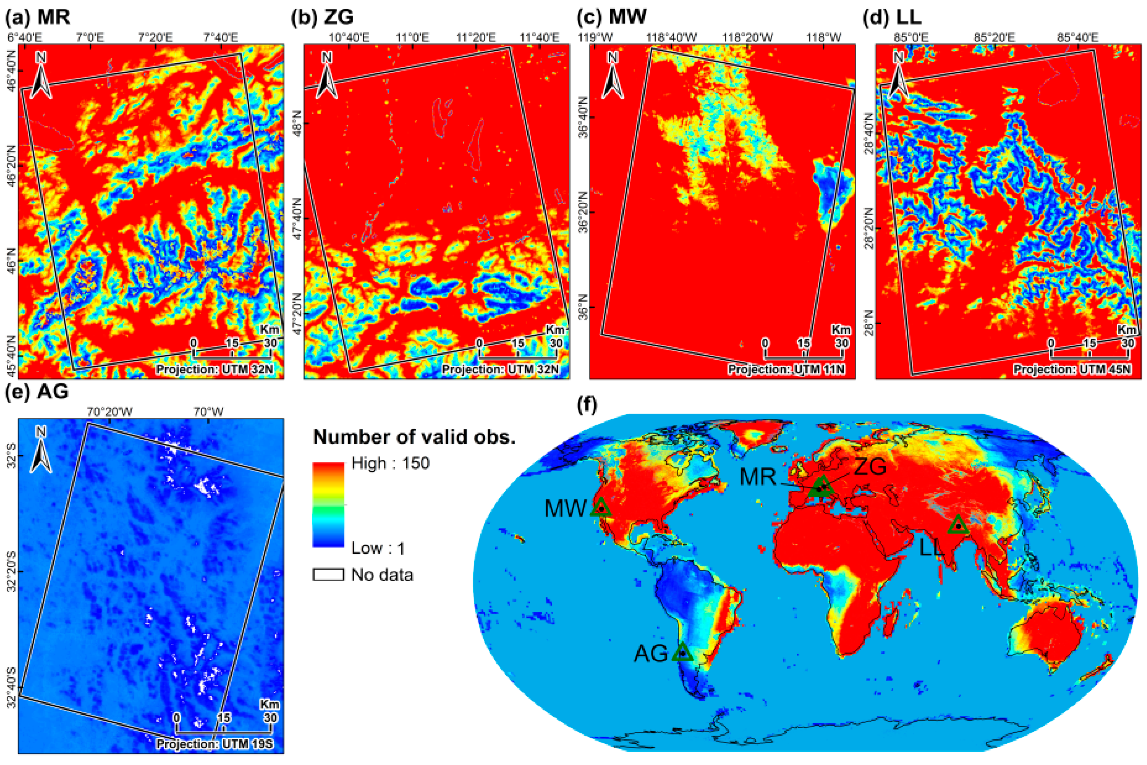
2.1. Study Areas

As this study intends to examine the global transferability of our approach, five regions around the globe were selected, as shown in Figure 1, where land cover types for each region is shown (with detailed information presented in

Table 1. Attributes of five selected study including Monte Rosa (MR), Zugspitze (ZG), Mount Whitney (MW), Landtang Lirung (LL), and Aconcagua (AG) areas along with their location, mountain range, country, and their highest peak.

Test Sites	1 (MR)	2 (ZG)	3 (MW)	4 (LL)	5 (AG)
Hemisphere	North	North	North	North	South
Continent	Europe	Europe	Northern America	Asia	Southern America
Mountain range (Country)	Alps (Switzerland)	Alps (Germany)	Sierra Nevada (United States)	Himalaya (Nepal)	Andes (Argentina)
Highest peaks (Height)	Monte Rosa (4634 m)	Zugspitze (2962 m)	Mount Whitney (4421 m)	Langtang Lirung (7234 m)	Aconcagua (6960 m)
Nearby city	Lausanne	Munich	Bakersfield	Kathmandu	Santiago

). Because one of our objectives is to compare the influence of different land cover types on the SCE detection, we selected regions in different continents, mountain ranges, and elevation zones, increasing the overall land cover diversity.

2.2. SAR Data

As this study aims at using openly accessible data sources, Sentinel-1 imagery provided by the European Space Agency (ESA) were employed. The conventional interferometric wide swath (IW) acquisition mode was used in this study. Both level 1 Single Look Complex (SLC) and Ground Range Detected (GRD) products were used, with the latter merging all sub-swath and de-bursting.

To validate our algorithm across different years and months/seasons, a total of three datasets (including one for the first hydrological year and two for the second hydrological year) were selected for each study area (details are shown in Figure 2 and

Table 2. Summary of the SAR data (Sentinel-1, S1) and optical data (Sentinel-2, S2; Landsat-7/8, L7/8) used for training and validation set of this study. Note: reference image of each region for calculating wet snow cover extent (SCE) is marked with an asterisk (*); optical images employed in validation set are included in brackets after the used SAR image dates.

Training Set (First Hydrological Year)	Validation Set (Second Hydrological Year)
	Month 1 (Month not Included in Training Set)	Month 2 (Month Included in Training Set)
Test Site 1: Monte Rosa (MR) (Sentinel-1A, Ascending, relative orbit number: 88) (Landsat-7/8, path: 195, row: 28)
2016 November 17–29	2018 March 12–24 (L7: March 23)	2018 May 11–23 (L8: May 18)
2017 February 09–21
2017 May 16–28
* 2017 August 08
Test Site 2: Zugspitze (ZG) (Sentinel-1A, Ascending, relative orbit number: 117) (Landsat-7, path: 193, row: 27) (Sentinel-2, tile number: T32TPT)
2016 November 07–19	2018 March 14–26 (L7: March 25)	2018 May 13–25 (S2: May 07)
2017 February 23–Mar 07
2017 May 18–30
* 2017 August 10
Test Site 3: Mount Whitney (MW) (Sentinel-1A, Ascending, relative orbit number: 144) (Landsat-7, path: 41, row: 35)
2017 February 25–Machr 09	2018 March 04–16 (L7: Mar 16)	2018 May 03–15 (L7: May 03)
2017 April 02–14
2017 May 08–20
* 2017 August 12
Test Site 4: Landtang Lirung (LL) (Sentinel-1A, Ascending, relative orbit number: 85) (Landsat-7, path: 141, row: 40)
2017 February 09–21	2018 February 28–March 12 (L7: Mar 13)	2018 May 11–23 (L7: May 16)
2017 April 10–22
2017 May 16–28
* 2017 August 08
Test Site 5: Aconcagua (AG) (Sentinel-1B, Descending, relative orbit number: 83) (Landsat-7/8, path: 233, row: 82)
2017 May 10–22	2018 June 10–22 (L8: Jun 13)	2018 May 05–17 (L7: May 04)
2017 August 14–26
2017 November 06–18
* 2018 January 29

). In order to represent snow cover conditions as well as to maximize the similarity of period sample used in each region, the months of November, February and May of the first year were selected in each region. However, for Mount Whitney (MW) and Landtang Lirung (LL) sites, the months of February, April, and May were chosen instead. This is due to the fact that in the MW and LL regions, the imagery was stable only after February 2017, as a result of a much rarer revisiting frequency of Sentinel-1, according to their orbit design, in comparison to European regions. Regarding Aconcagua (AG), the only site located in the southern hemisphere, has opposite season, the corresponding months samples were used. Two different months of imagery were used for external validation in examining the month-dependency of the established model set.

2.3. Auxiliary Data

In addition to SAR-derived information, it is also critical to include both land cover as well as topographical information for building a model for the total SCE classification. Considering the global availability, accessibility and data sustainability, we relied on the version 4 of the digital elevation model (DEM) based on National Aeronautics and Space Administration (NASA)’s Shuttle Radar Topographic Mission (SRTM), as well as the land cover data provided by ESA Climate Change Initiative (CCI) product version 2.0.7. SRTM DEM was used to derive elevation, slope, and aspect and curvature topographical information.

Even though the Advanced Spaceborne Thermal Emission and Reflection Radiometer (ASTER) DEM has 30 m spatial resolution and global coverage, which is better when compared to the SRTMv4 DEM (around 80% global coverage and 90 m spatial resolution), SRTM was chosen as a source for the DEM as it provides higher vertical accuracy [35,36,37,38]. For land cover data, we selected the ESA CCI land cover product because CCI not only provides a global coverage with 300 m resolution and quality flags denoting the number of valid observations used for classification, but has also been annually updated since 1992, with the latest update in 2015.

The ESA CCI land cover product typology follows the land cover classification system (LCCS) defined by the United Nations (UN) Food and Agriculture Organization (FAO) [39]. It originally categorizes 37 different land cover types including some detailed distinguishments, such as different ratio of mosaic tree and shrub with herbaceous cover; hence all original 37 classes were re-categorized to 16 classes for our study (definition shown in Appendix A), to maintain class differences while avoiding complexity.

To train and validate our models, DLR’s Global SnowPack [14] was employed as it provides daily full globe SCE in 500 m spatial resolution without the influence of cloud coverage or polar darkness. Moreover, its daily SCE availability allows for a same-day training and validation when the Sentinel-1 scenes are acquired.

3. Methodology

3.1. SAR Imagery Processing

The processing of SAR-based observations requires several steps in order to support the three mainstream SAR-based SCE detecting approaches comprising backscattering, InSAR, and PolSAR-based methods.

For backscattering-based information, each GRD SAR image was subset to the extent of the study region. Each image was calibrated, had its thermal noise removed, and underwent speckle filtering with Lee sigma filter [40] (7 × 7 window size). It was then corrected for terrain flattening and distortion with the SRTM DEM, and converted to decibel (dB) units. Finally, each season’s SAR dB dataset was set in relation to the summertime’s reference dB image (i.e., theoretically bare/snow-free ground) (Table 2). It is important that, as the quantitative analysis is involved (ratio), the original intensity value or digital numbers (DN) of GRD images need to be calibrated. This is to represent the genuine brightness value based on the incidence angle information [41].

Two SLC images were co-registered for InSAR processing to estimate the coherence value. As IW mode Sentinel-1 imagery is sensed at TOPS mode, it is necessary to respectively split each sub-swath and merge each burst, before and after co-registration. The coherence map was then terrain corrected to remove distortions. For InSAR, the temporal baseline between master and slave images should be shortened to reduce the magnitude of temporal variability that may affect the coherence value considerably [42]. Thus, the temporally nearest SAR imagery of a selected master scene was used as slave image.

Finally, for polarimetric information, each SLC image was calibrated, debursted, and the polarimetric matrix was constructed. As the employed Sentinel-1 IW mode imagery only provides dual polarizations (VV and VH polarizations in all five study regions), the incoherent polarimetric C2 (2 × 2) complex covariance matrix formed by co- and cross-polarized complex scattering amplitudes was used [43,44]. The refined Lee filter [45], with 7 × 7 window size, was then applied to de-speckle, and a decomposition was performed before the final terrain correction. In the presented study, the H/A/α decomposition proposed by Cloude and Pottier [27] was selected due to the availability of dual-polarizations as well as the intensive employment frequency and its viability to detect SCE [46,47,48,49]. Under the commonly used assumption of reciprocal targets (i.e., scattering amplitude of VH and HV are the same) [44], H/A/α decomposition utilizes the eigenvalues and eigenvectors calculated from the coherency matrix, which then composes the H/A/α, representing the entropy (randomness of depolarization of scattering type), anisotropy (normalized difference of importance of scattering type), and scattering angle (dominant scattering angle and type). The comprehensive descriptions of decomposition can refer to [27,44].

3.2. Total SCE Detection

3.2.1. Random Forest Classification

As the aim of this study is to detect snow cover on the land surface of various regions around the globe, a simple tuning classifier which is capable of efficiently solving a two-class classification problem is necessary. According to the Global Observing System for Climate (GCOS) [50], a spatial resolution of at least 100 m is necessary for snow cover mapping in mountain regions. Therefore, it was set as the output of the implemented model setup. In this study, the random forest (RF) [51] was chosen to classify snow cover based on SAR observations. Compared to other supervised classifiers, RF has multiple advantages, including a relatively short training time, low computation load, capability to handle high dimensional data with missing values, support of parallel processing, simple tuning of parameters, avoiding of over-fitting, providing importance indexes of input variables, and providing an internal quality index (out-of-bag (OOB) error) [51,52,53,54,55,56,57]. Due to these advantages, RF has been widely applied to many remote sensing-based classification topics [32,57,58,59,60,61,62,63,64]. However, it is still surprising that, so far, studies relying on RF classifiers for SCE mapping are very rare.

In the present study, the two required tuning parameters for saving memory consumption and computation time while yielding the highest classification performance after several test runs, that is, the parameters of the number of trees L and number of random features assigned to each tree ${\theta }_k$, are respectively set to 600 and the default value (square root of total feature numbers). Although several studies demonstrated that L has less influence than ${\theta }_k$ on the classification accuracy [57,65,66], different L values were tested (ranging from 50 to 1000) in Monte Rosa (MR) region and the resultant classification accuracy and processing time are presented in Appendix A. It was found that the RF model with 600 trees can efficiently achieve on optimized accuracy. This finding agrees with previous studies suggesting that a tree number of around 500 is generally sufficient [67,68].

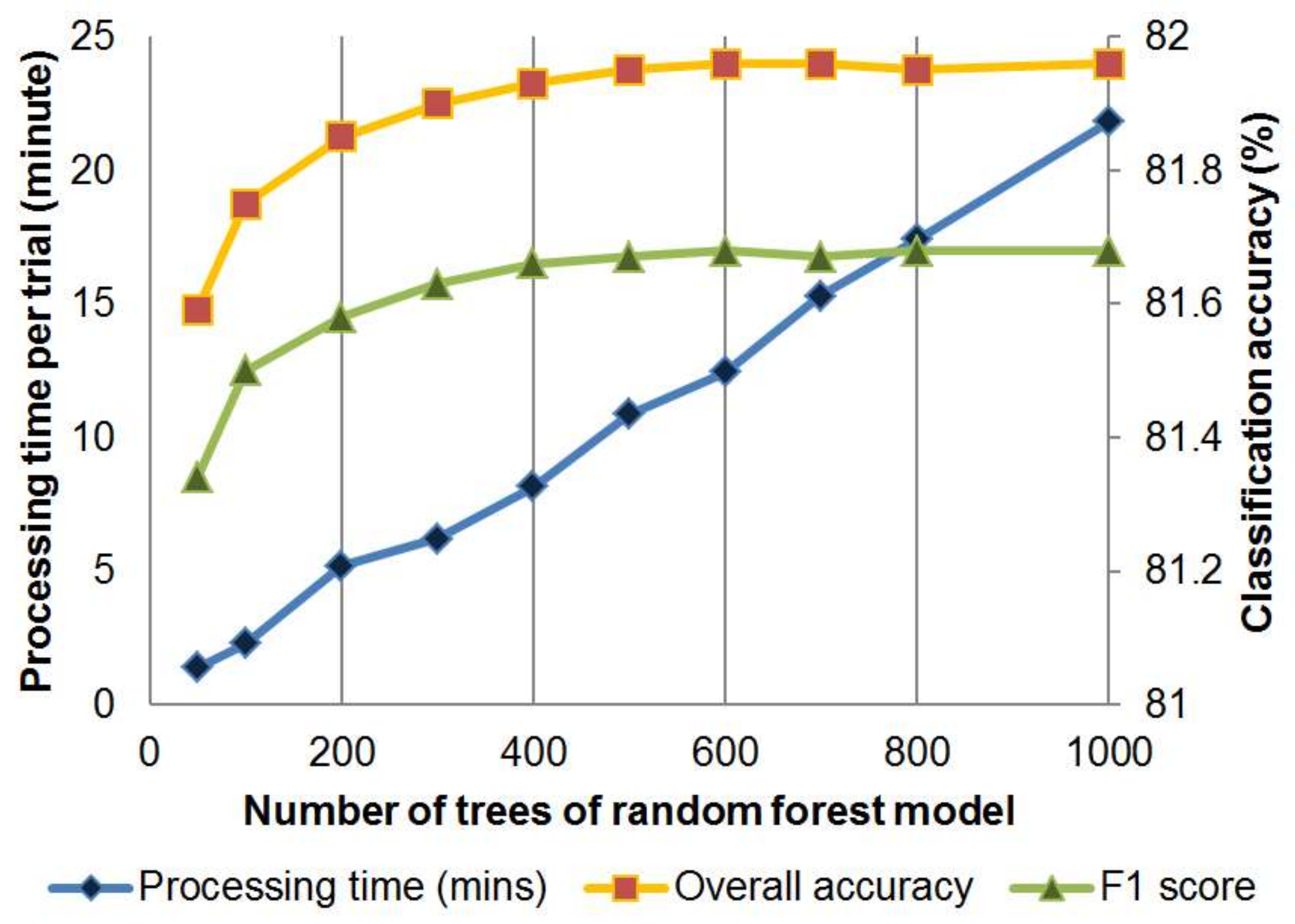
3.2.2. Random Forest Model Setup

For building the RF models, the selected input variables included: (1) SAR-based observations (backscattering ratio, interferometric coherence, and polarimetric H/A/α parameters, as mentioned in 3.1); (2) topographical information: elevation, slope, aspect, and curvature derived from SRTM DEM; (3) land cover classes (ESA CCI land cover product); and (4) total SCE (Global SnowPack daily SCE).

The RF models were established separately for each land cover class. Namely, each modelling trial consists of N RF models, with N referring to the number of land cover classes in the study region. To test the influence of the three SAR observations and the four topographical factors on the RF performance, they were combined in varying setups. Firstly, uni-, dual-, and three SAR observation-combined based models were tested. Then, the highest accuracy model was added with single and all topographical information. Eventually, the best observation-factor combination model was then applied in two individual RF model scenarios. In the first case, each region’s first year’s data was used to build the model for each region individually, which were then correspondingly applied to the region’s second year’s data. Consequently, in the second case, the input data of all test regions were merged from the first year’s data to build one aggregated model, which was applied to the second year.

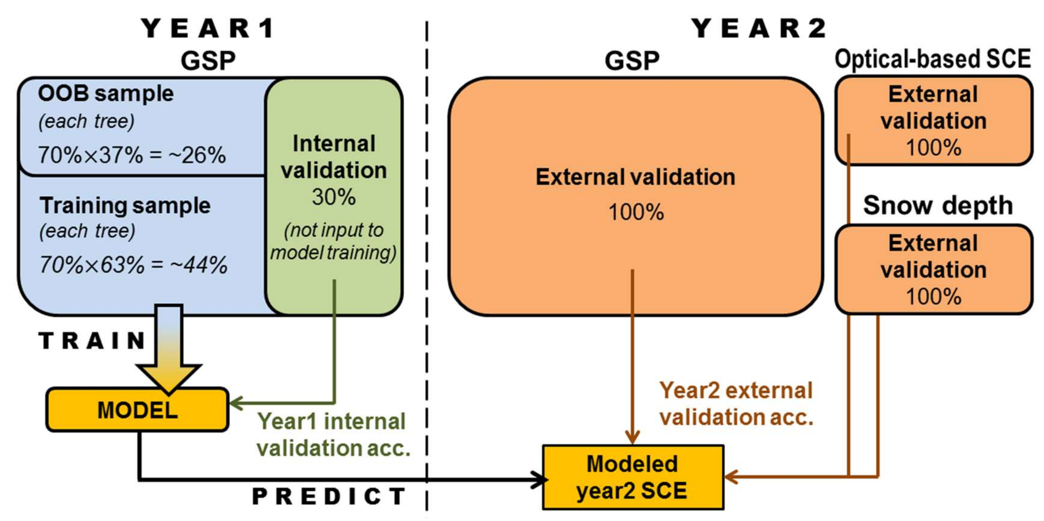
3.2.3. Data Splitting for Model Training and Validation, Calculation of Accuracy Evaluation Measurements

To establish the RF model as well as to achieve a comprehensive validation, in the presented study many different sources of data were used, including GSP, optical-based SCE, and snow depth data of meteorological stations. The overall data splitting for each region’s land cover class’s model training and validation is illustrated in Figure 3.

First, to train the RF model, 70% of the pixels of the first year’s data (including SAR-based observations and topographical factors mentioned in 3.2.2) were randomly selected and facilitated to build the model. The established model was then internally validated with 30% of the first year’s GSP data, which were manually omitted from building the model. It must be noted that the OOB samples, which account for around 37% of input data, which were automatically not employed in the training sample when building the RF model and assigning features to the model trees, were not used for cross-validation in the presented study. The coarse resolution of GSP (500 m) would inevitably lead to spatial autocorrelation between training and OOB samples. Namely, the value between two sample sets are dependent, which could lead to overestimation of OOB accuracy [67].

Then the established RF model (only trained by first year’s GSP data) was used to predict the SCE of the second year, which was then validated with additional external validation sources, including the second year’s GSP (two sets of data, as shown in Table 2), Landsat/Sentinel-2-based SCE, and meteorological data.

When comparing the different model inputs and setups, one of the most critical steps is to evaluate the specific model performances. Hence, an accuracy assessment was introduced, including overall accuracy, F-measure [69], and “Area Under the Receiver Operating Characteristic Curve (ROC)” (AUC) [70]. These indexes provide different evaluation aspects [71,72] as overall accuracy. F-measure focuses on minimizing the number of errors based on thresholding and qualitative evaluation. In contrast, AUC’s purpose is to show how accurate the classes are separated, by checking how the model ranks the examples. Moreover, as it is commonly known that forest-covered areas could produce erroneous results (based on SAR data snow cover classifications [47,73,74,75], the abovementioned accuracy measurements were also used to calculate non-forested regions separately (the criteria of forest type listed as Appendix A) in order to examine the influence of vegetation.

Considering the overall accuracy, F-measure, and AUC, all of them can be derived from the confusion matrix. In this study, overall accuracy is defined as:

$$\begin{array}{c}Overall Accuracy=\\ \frac{pixels within true total SCE classified as total SCE + pixels in snow free classified as snow free}{all pixels}\end{array}$$

(1)

The F-measure score (a.k.a. F1 score), is a composed weighted measurement which considers both recall as well as precision. In this study, these accuracy indices were calculated as following:

$$Precision=\frac{pixels within true total SCE classified as \mathrm{total} SCE}{pixels classifed as total SCE}$$

(2)

$$Recall=\frac{pixels within true total SCE classified as \mathrm{total} SCE}{pixels within true total SCE}$$

(3)

$$F1 score=\frac{precision\times recall}{precision+recall}$$

(4)

The last quality index that is calculated to evaluate the performance of the model is the AUC score, which is based on ROC. The ROC curve is plotted with false positive rate and true positive rate on the x- and y-axis, respectively. The specificity can be defined as:

$$Specificity=\frac{pixel not in true total SCE classified as not total SCE}{pixel not in true total SCE}$$

(5)

ROC can be interpreted as the probability of ranking randomly selected actual positive samples over randomly selected negative samples. AUC is defined as the area between the ROC and y = x function, which has a value range from 0.5 to 1.0. According to Metz [76], AUC values range from 0.5 to 0.6, 0.6 to 0.7, 0.7 to 0.8, 0.8 to 0.9, and 0.9 to 1.0, representing bad, satisfactory, good, very good, and excellent model performance, respectively.

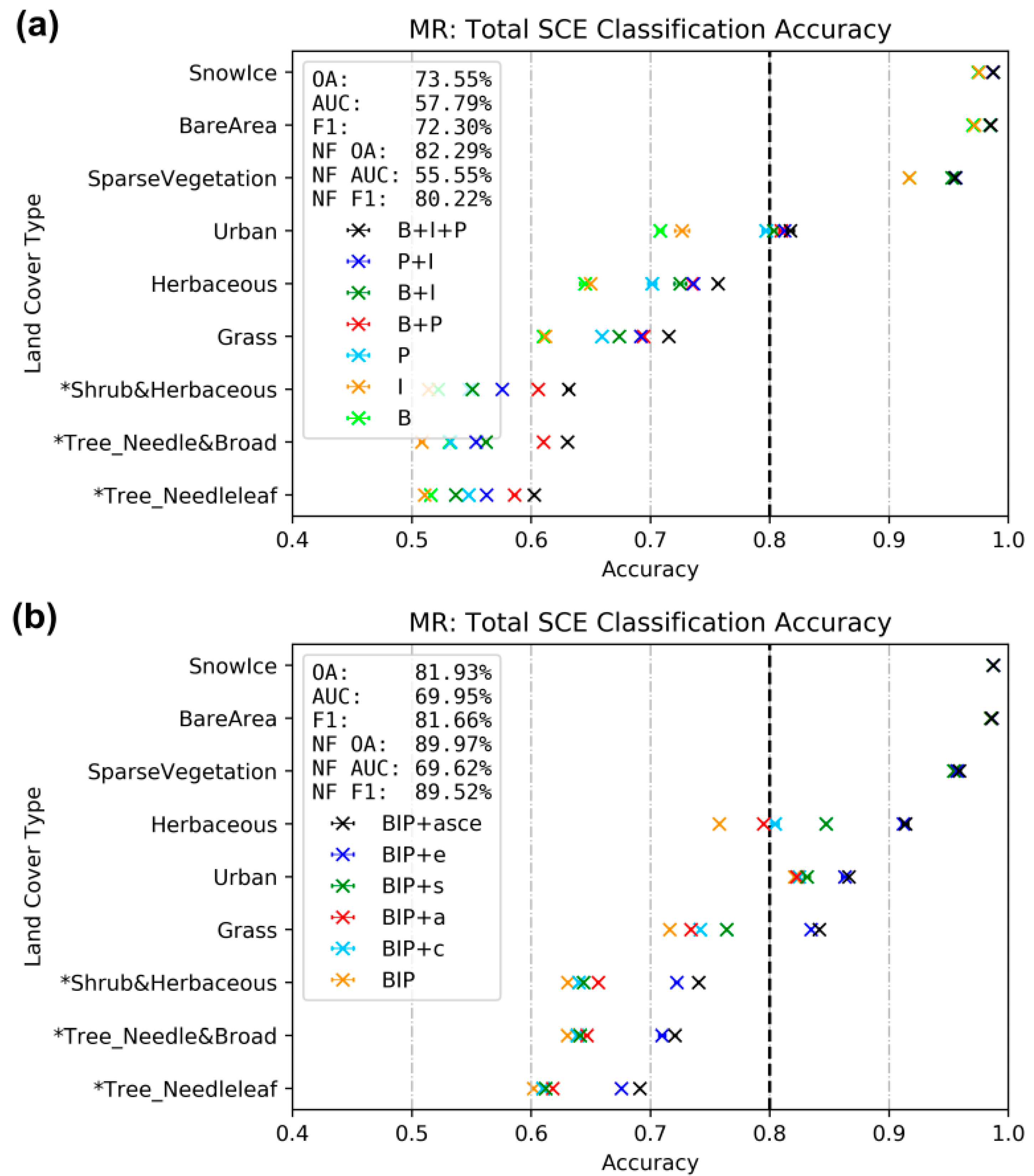
3.2.4. Tests for Selecting the Optimized Model Input Variables

As described in Section 3.2.2, the possible inputs for the implemented model to detect total SCE include SAR-based observations (backscattering ratio, InSAR coherence and PolSAR H/A/α parameters, abbreviated as B, I and P), topographical parameters (elevation, aspect, slope, and curvature, abbreviated as e, a, s, and c), and land cover information originating from the CCI land cover product. To select the optimized input combination for the model, Monte Rosa (MR) in the Swiss Alps was chosen as a pilot study site for an in-depth accuracy assessment, as it is characterized by complex topography and land cover.

To test the influence of the SAR parameters on the model performance, different combinations of SAR-based observations were employed to train MR’s model set. To assess their uncertainties, 20 iterations were processed for each trial. Resultant accuracy assessments are illustrated in Figure 4a. It was obvious that for all land cover classes, the combination of all available SAR parameters (B + I + P) produced the highest accuracy. When relying only on one SAR-based observation, using P leaded to higher classification accuracy than relying on I or B. The accuracy improvement between using only single SAR parameters and the combination of all available parameters (B + I + P) was significant. Moreover, it was observed that for land cover classes that pose considerable challenges in detecting snow cover using SAR (e.g., forested areas), combining all available SAR parameters leaded to a significant improvement of classification accuracy.

For evaluating the influence of topographical parameters on the model performance, elevation (e), aspect (a), slope (s), and curvature (c) were added as input parameters to the ML approach separately. Their influence on the classification accuracy is presented in Figure 4b. Results showed that by successively adding more topographical parameters the performance of the model increased, leading to its highest performance if all parameters are added collectively (“asce” case in Figure 4b). The overall accuracy for all land cover classes could be improved by around 8.4%, while the F1 score improved by 9.4% when compared to using only the combination of B + I + P as inputs. Even in non-forested areas, the accuracy (non-forest classes’ overall accuracy (NF OA)) raised by around 7.7%. Additionally, the AUC value could be improved by more than 12%. Of all tested topographical parameters, elevation had the biggest impact on the model performance. For example, using only B + I + P to classify snow cover within the mixed shrub and herbaceous land cover, the accuracy only reached around 0.62. This value could be improved to 0.72 by only adding elevation (e) as an auxiliary input. By adding the remaining three topographical parameters (s + a + c), the accuracy increased to 0.74. Testing the influence of different combinations of input parameters (SAR as well as topographic), it became clear that the combination of all available SAR-based observations and all topographical parameters leaded to the best model performance for classifying total snow cover. The same tests have been performed for all test sites listed in Table 2, which are not illustrated here for clarity, but leading to the same results as for the Monte Rosa test site. Therefore, all available SAR-based observations and all topographical parameters have been used as model inputs for the subsequently presented results.

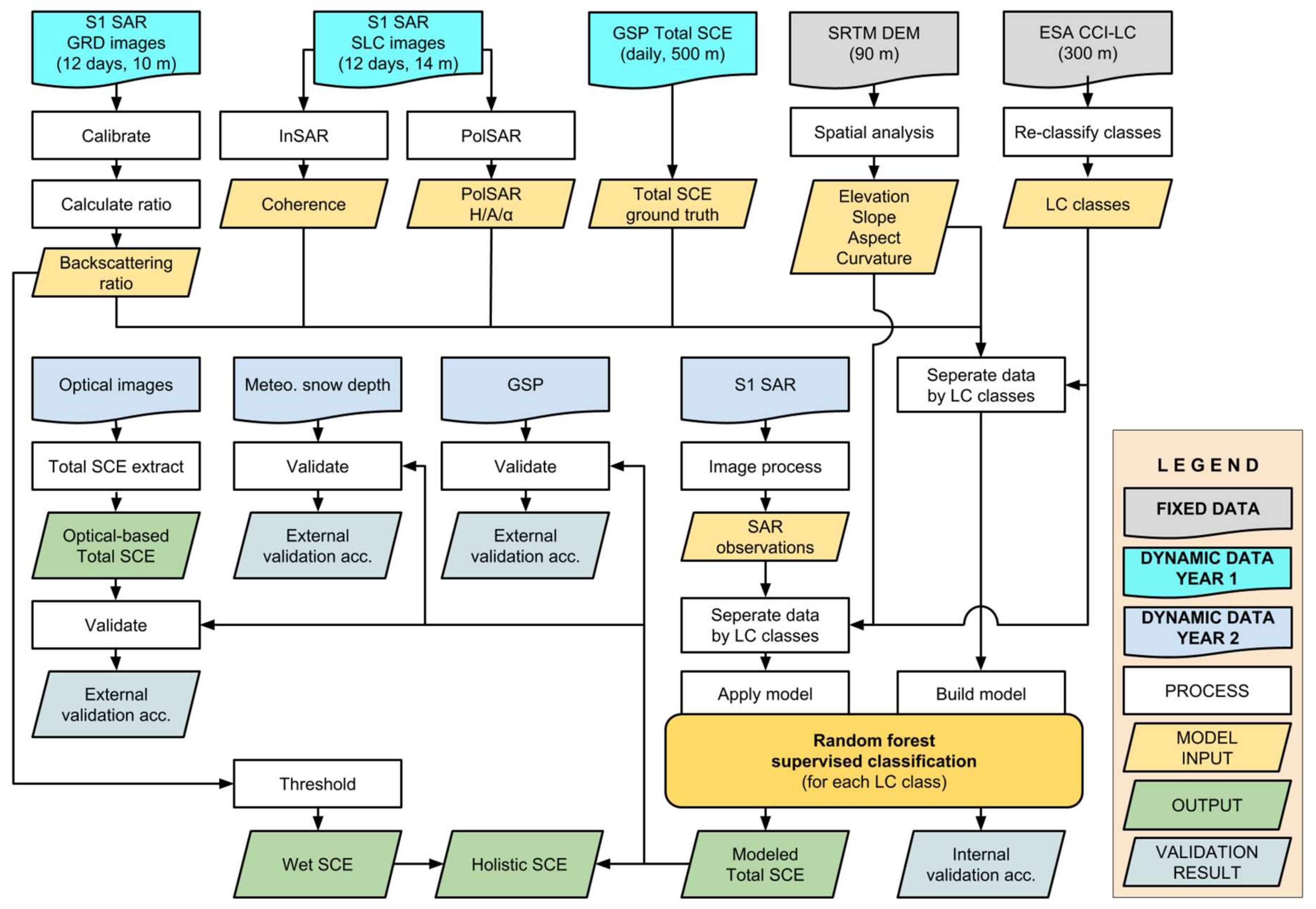
3.3. Holistic (Total + Wet) SCE Detection and Overall Workflow Overview

The wet SCE detection was performed, in addition to the RF-based classification of the total SCE, in order to exploit the full potential of the SAR data and to discriminate between wet and dry snow. To map the wet SCE, the backscattering coefficient-based “Nagler’s method” was applied. As summarized in the introduction, this method requires two SAR images sensed at snow-covered and snow-free conditions. It utilizes a backscattering threshold (−3 dB) to the ratio map of the two images for detecting the wet SCE. In the present study, according to the feasibility of using a cross-temporal reference image, proved by Luojus et al. [20], both years’ SAR data observed during the snow-covered season were combined with the reference scene (summertime observation) of the first year (Table 2).

The overall workflow of mapping total SCE, by applying a supervised RF classification model set as well as detecting wet SCE with “Nagler’s method”, is illustrated in Figure 5.

4. Results

Based on the optimized input variable combinations tested in Section 3.2.4, the same modelling approach was applied to all five study areas. Additionally, to examine the transferability of the model setups, the results were comprehensively validated with different data sets (Landsat/Sentinel-2 and in-situ snow depth information). Finally, the holistic (total + wet) SCE was derived based on the modeled total SCE and wet SCE calculated from “Nagler’s method”.

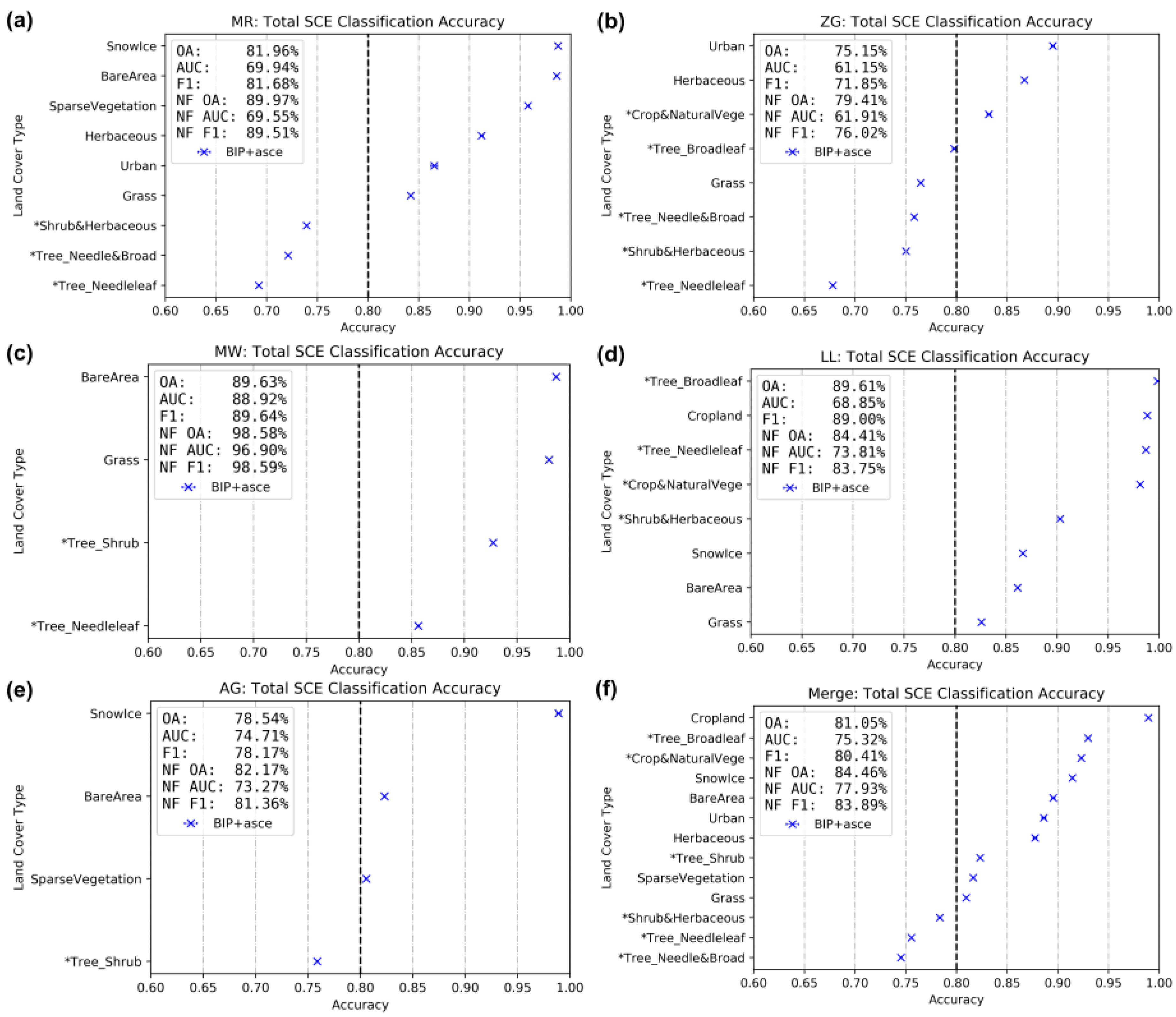
4.1. Accuracy Assessment of Modeled Total SCE

As presented in Section 2.1, five different study areas located around the globe were selected and applied with the proposed model. The total SCE mapping model set can be trained by either: (1) Using each region’s data to train an individual model set and; therefore, training a region-dependent model set; or (2) merging all regions’ data to train one universal model set, which was then applicable for all regions simultaneously. Depending on the intentional application of the model, it might be sufficient to have a spatially confined model that only works for a specific region. However, if it is required to derive snow cover information for several varying locations, a universal model set has to be implemented. For both cases, the performance of the model has to be known and; therefore, has to be assessed.

For the first (individual) case, the results of the accuracy assessment are presented in Figure 6a–e. The overall accuracy of Monte Rosa (MR), Zugspitze (ZG), Mount Whitney (MW), Landtang Lirung (LL), and Aconcagua (AG) were around 80%, 75%, 90%, 90%, and 80%, respectively. The F1 score for each test site was higher than 70%. AUC scores for all regions were around 70% or higher which indicated a good model performance; with the exception of ZG, with around 60%, which was still satisfying. The amount and distribution of land cover vary between the test sites and affect the overall accuracy of the model performance. The complexity of land cover types within the CCI land cover product used as auxiliary data in this study was considerably higher in the Europeans Alps and Asian Himalaya when compared to the Andes and Rocky Mountains (see Figure 1). As already reported in earlier SAR-based snow cover studies [17,18], lower accuracy values are achieved in grassland as well as forested areas (classes marked as * in Figure 6), with the exception of the LL test site. To examine the negative effect of grassland and forest areas of the classification performance, the overall accuracy, F measure, and AUC score values have also been calculated for non-forest classes (indicated in Figure 6 and abbreviated with NF OA, NF F1, and NF AUC).

As outlined above, building individual models for each test site separately can guarantee a more customized classification with higher accuracy. The overall accuracy of these individual cases including forests and grassland ranged from 75.2% to 89.6% (of which 79.4%–98.6% excluding forests and grassland) with F1 scores ranging from 71.9% to 89.6% (of which 76.0%–98.6% excluding forests and grassland, see Figure 6a–e). All input data were also merged to build a universally applicable model, which showed only slightly lower accuracy values of 81.1% of the overall accuracy (of which 84.5% excluding forests and grassland) and an F1 score of 80.4% (of which 83.9% excluding forests and grassland, see Figure 6f). These values proved a good model performance. This evaluation revealed the robustness of the classification approach proposed in this study whilst merging all input data to create a globally transferable model setup; even if the model was trained universally. The sturdiness can also be exposed from the neglected accuracy difference of 20 trials for each land cover class of each region.

4.2. External Validation

Although previous studies often neglect the importance of a detailed validation approach, it is indispensable to comprehensively examine the robustness and correctness of a proposed model with internal and external validation efforts. Consequently, several validation steps have been incorporated into the presented study. It complements the internal validation illustrated in Section 4.1, with addition to external validation based on the GSP, optical-based SCE, and in-situ snow depth data, as illustrated in the data splitting of Figure 3 and workflow of Figure 5. The results of these accuracy assessments are presented in the following sections.

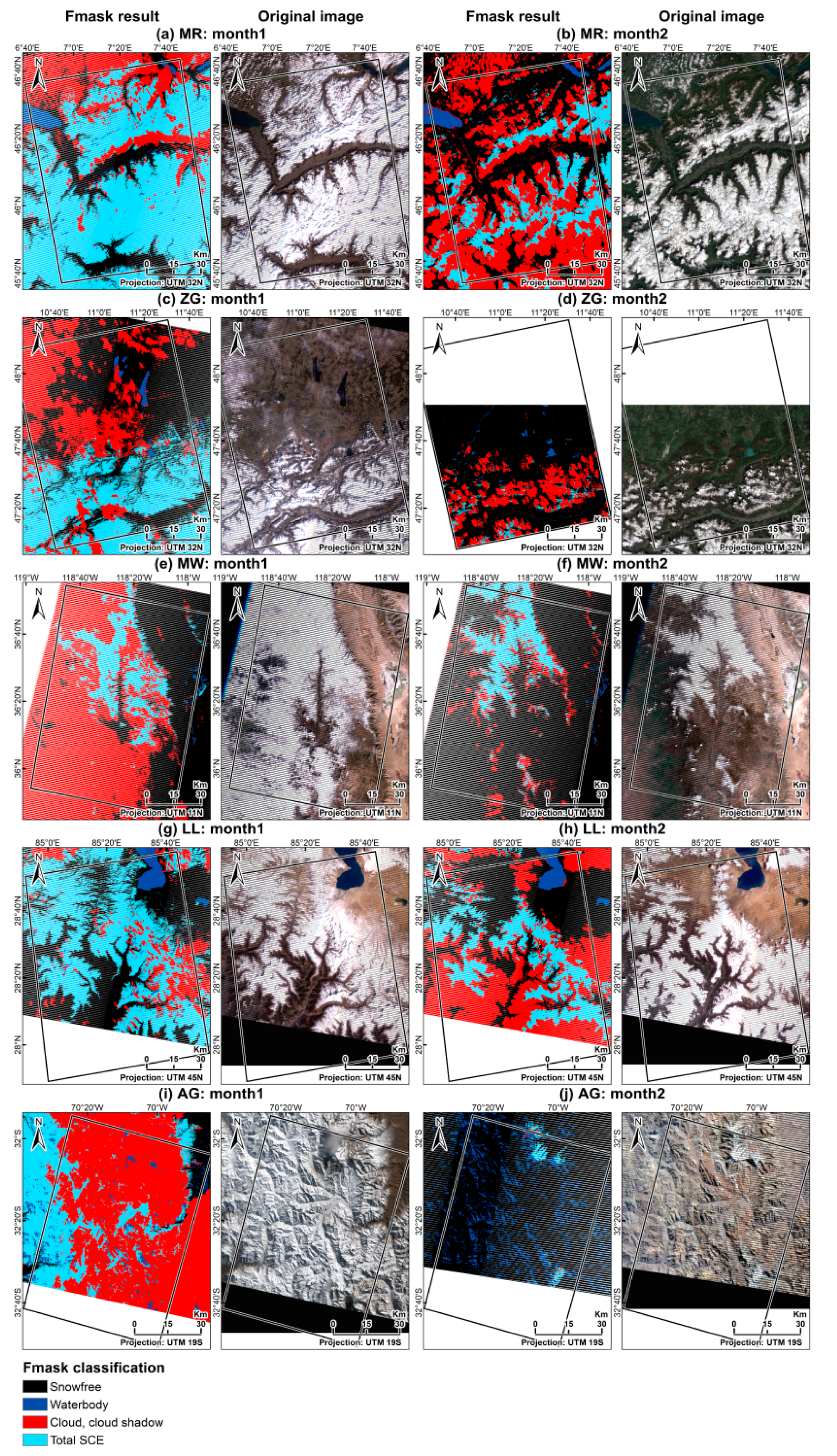
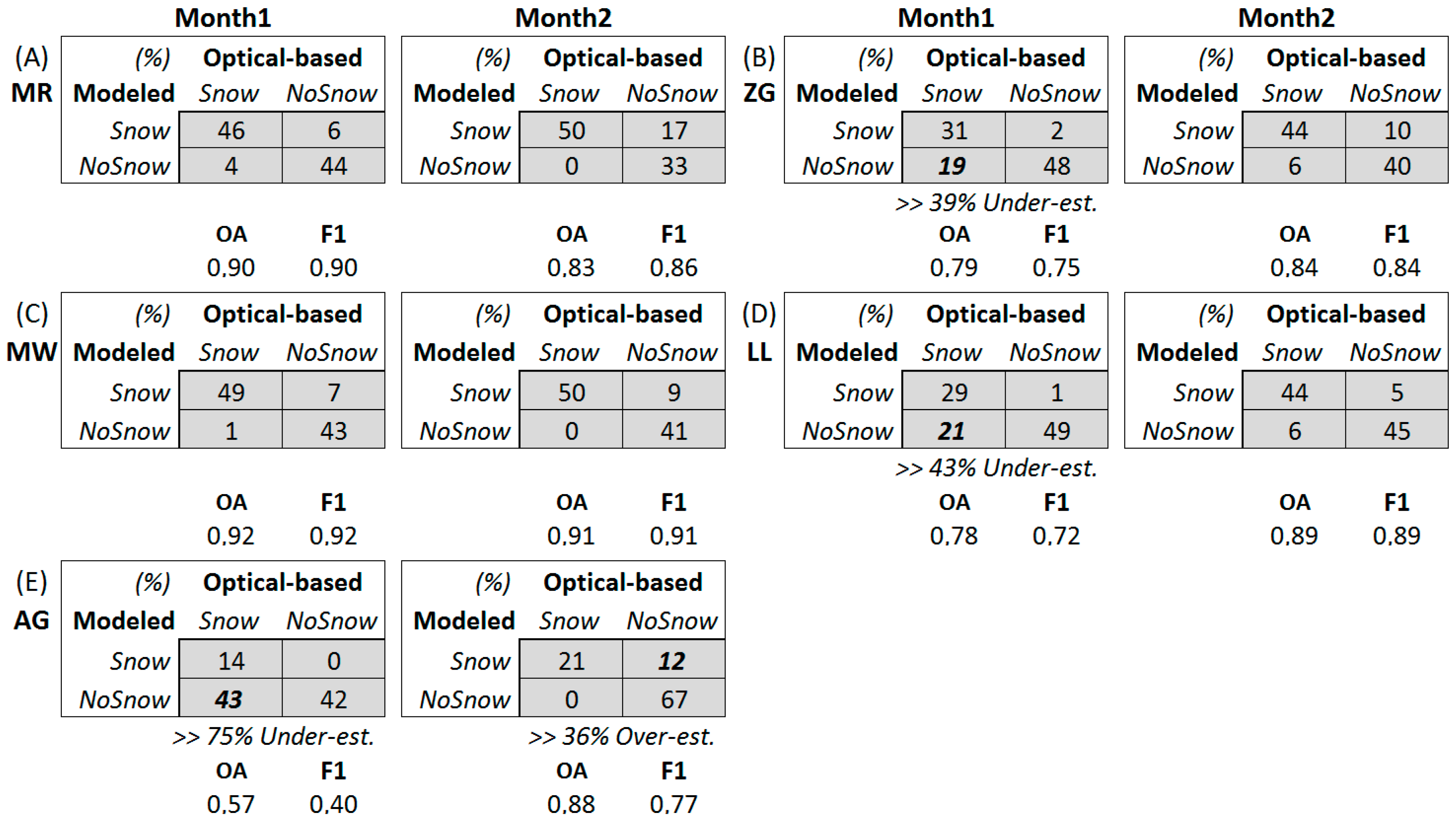
4.2.1. Results of the External Validation with the Global SnowPack and Landsat/Sentinel-2-Derived Snow Cover Maps

In order to examine each land cover types’ influence on the model’s accuracy, the comparison between the “training accuracy” (the overall accuracy of the internal validation, calculated based on 30% of the first year’s data manually kept (Figure 3)) and the “validation accuracy” (the overall accuracy of the external validation, calculated based on the second year’s GSP) were calculated and presented as blue and red bars in Figure 7, respectively. Most of the land cover types showed a slightly lower accuracy for all test sites of the second-year validation accuracy, with the exception of the ZG region. However, almost all land cover types within all study areas were still characterized by a satisfying accuracy (>0.6), with the exception of forested classes of the MR region. This affirmed the robustness of the employed model set.

The 500m spatial resolution GSP product may not accurately depict the actual SCE in mountain regions due to missed pixel effects and the negative influence of temporal interpolation for cloud-gap filling. Therefore, in addition to this product, higher resolution optical imagery originating from Landsat-7/8 (30 m) and Sentinel-2 (20 m) were also employed to derive SCE for validation. All available observations from these two sensors were screened for suitable data (i.e., cloud-free). The observations chosen for processing are listed in Table 2. The aim is to keep the observation date of the optical sensor as close as possible to the SAR data’s date, which could be achieved for most cases with temporal gaps of less than one week.

To extract the optical-based total SCE, the Fmask algorithm was employed [77]. Fmask is an algorithm that aims to extract clouds, cloud shadows, snow, and waterbodies from Landsat 4–8 and Sentinel-2 imagery. Thanks to its mountainous Fmask function, which utilizes additional DEM information, the accuracy of mapping cloud shadow and removing terrain shadow in mountainous regions is significantly improved. For parameter setting, the dilation size of cloud, cloud shadow, and snow were set to 3, 3, and 0, respectively. The threshold for cloud probability was set to 10.0% for Landsat-7, 17.5% for Landsat-8, and 20.0% for Sentinel-2. The resultant total SCE and original true color composites for each study site are shown in Figure 8. Overall, the Fmask classification results were reasonable, except for AG region showing misclassification of waterbody. However, it was also obvious that there was still serious cloud contamination. Additionally, due to the orbit design and sensing swath of the satellites, the study area was not always completely covered by the Landsat/Sentinel-2 observation.

To compare two total SCE results (the SAR-based one based on the RF classification, and the optical-based classification based on Fmask), a total of 10,000 random points were equally distributed in both snow-covered as well as bare ground areas (5000 points each). The points were distributed based on the result of the Fmask product, excluding cloud-covered areas by treating them as no-data. Although some studies reported that Fmask may tend to over-estimate cloud [78,79], in the present random-point-allocating method it would not damage the reliability of validation. A confusion matrix as well as evaluation indexes (overall accuracy and F1 score) were then computed for each test site and each month of the second year, and the results of this assessment are presented in Figure 9. To simplify the interpretation, the numbers of points in each column/row of the confusion matrix were converted into a percentage of the total 10,000 points. All ten months’ cases showed good accuracy and F1 score (>0.72); except for month1 (month not used in the training of the first year, referring to Table 2) of AG region, which showed significant under-estimation. Under-estimation was also shown in non-used month (month1) of the first year in ZG and LL region. Furthermore, the month2 (month included in training set) of AG region showed a mild over-estimation.

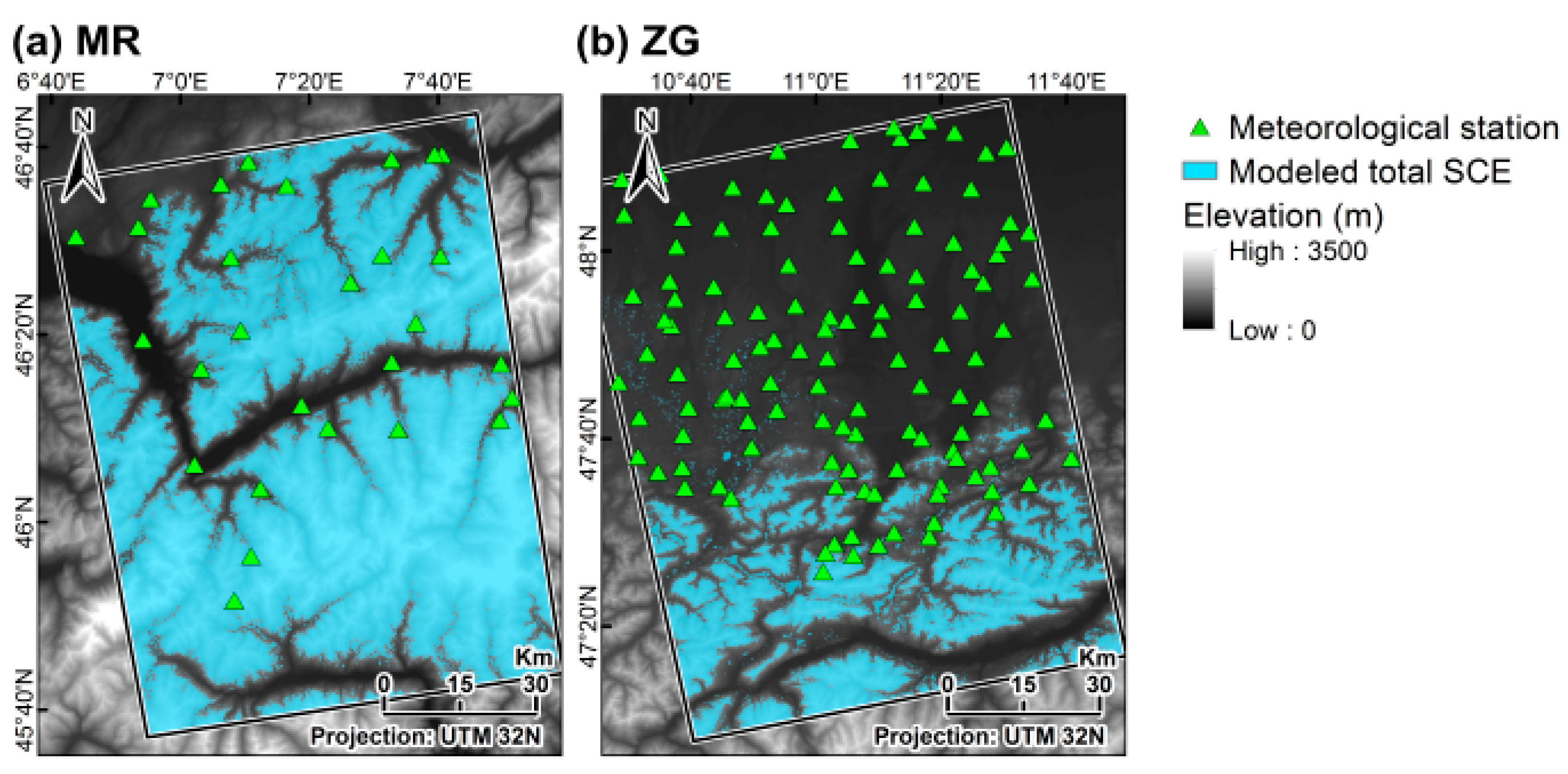
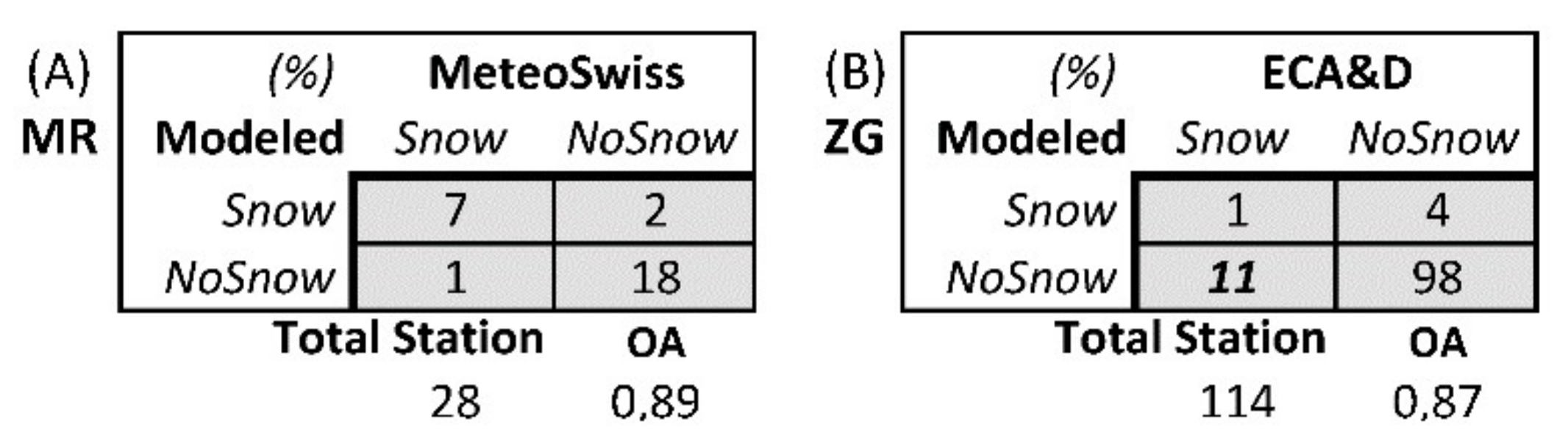
4.2.2. Validation Relying on In-Situ Data Originating from Meteorological Stations

In addition to the validation based on satellite observations, snow depth (SD) measurements originating from meteorological stations are available for some study areas. For the European region, few countries’ national meteorological agencies, for example in Switzerland, provide free access to these data. Additional measurements of daily SD are available from the European Climate Assessment and Dataset Project (ECA&D) [80]. The study sites MR and ZG were chosen to be validated with 28 stations of MeteoSwiss and 114 stations of ECA&D, respectively. The locations of the meteorological stations are illustrated in Figure 10. However, as more than 50% of the stations are located in relatively low elevation zones, which are generally completely snow-free in May, only March observations were validated for the presented study. For the study site MW, only one meteorological station was available, while for LL and AG, no suitable and freely accessible station data could be acquired. Therefore, these three regions were not validated with meteorological records. The confusion matrix, displaying the accuracy derived from the comparison of the SAR-based SCE classification with station data, is illustrated in Figure 11. Whilst not considering the skewed observations (station records contain less “snow-covered” data (i.e., SD higher than 0 cm)), both regions achieved overall accuracy values of more than 87%. However, a slight under-estimation can be found in the ZG region. This could be because there might exist a certain threshold of SD for the spaceborne SAR-based approach to detect that a pixel is snow-covered, such as 1 cm for MODIS snow cover product [81] and 2 cm for passive sensors [82].

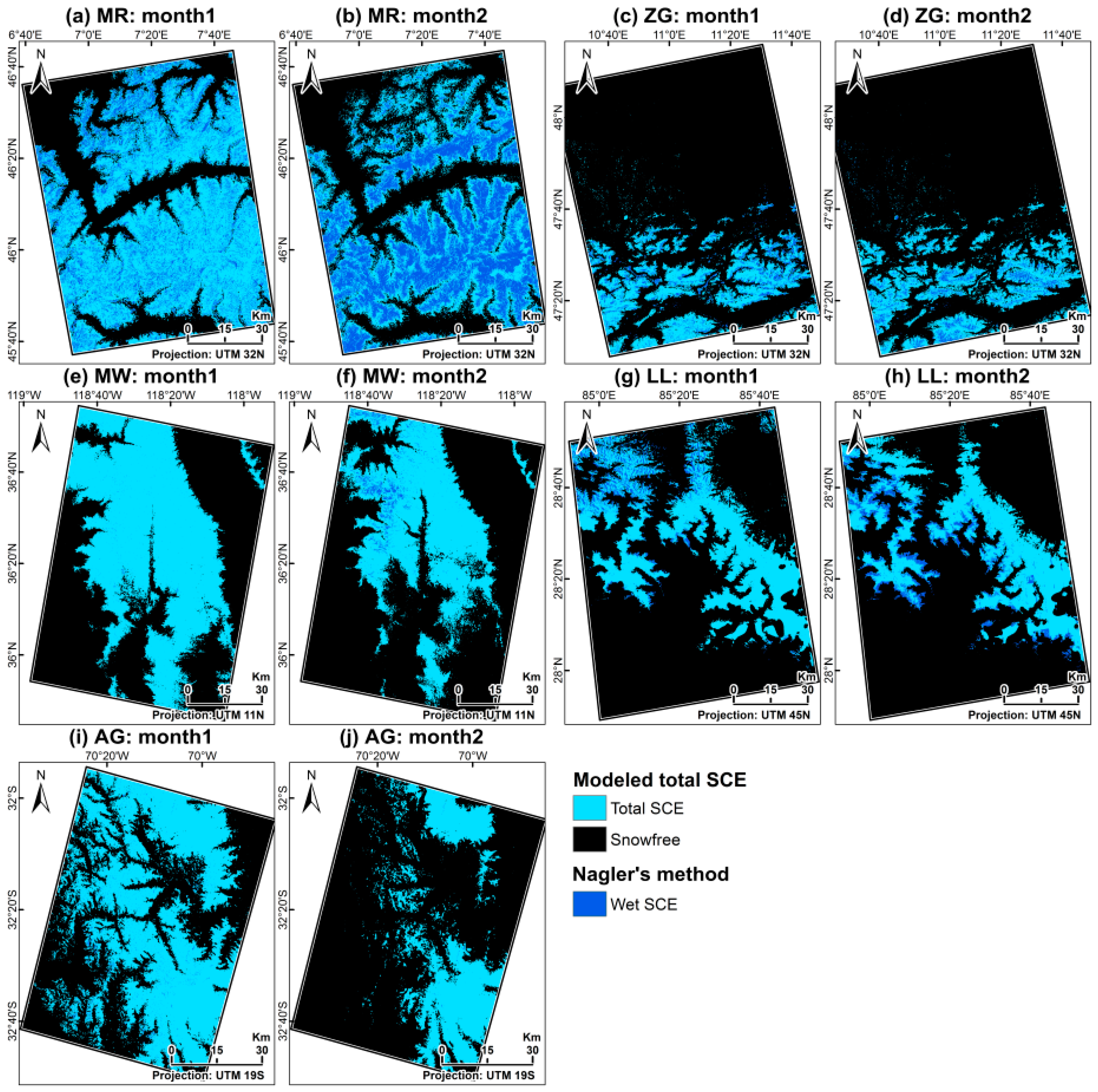
4.3. Holistic SCE Maps Including Discrimination between Wet and Dry Snow

According to the comprehensive internal and external validation approaches relying on different data sources, all study regions turned out to achieve reliable accuracy values; with the exception of AG region, which showed comparably weaker results. As the RF classification approach relied on training data originating from optical-based products (GSP), it is not possible to train for the discrimination between wet and dry snow. However, as this information is required, we also detected the wet SCE based on Nagler’s algorithm [17]. For the subsequent merge of the total SCE derived from the RF classification and the wet SCE derived from Nagler’s classification, the presence of wet SCE was only allowed for regions where the RF classification had successfully detected snow. Figure 12 contains the results of this merging approach for all test sites, including month 1 and 2, to illustrate the dynamics of SCE. During March (month 1, Figure 12a,c,e,g,i), the total extent of snow cover was larger but wet SCE was proportionally small. As snow melt proceeded during the spring time, wet SCE increased (month 2, Figure 12b,d,f, and h, with AG region constituting an exception) while the total SCE decreased.

5. Discussion

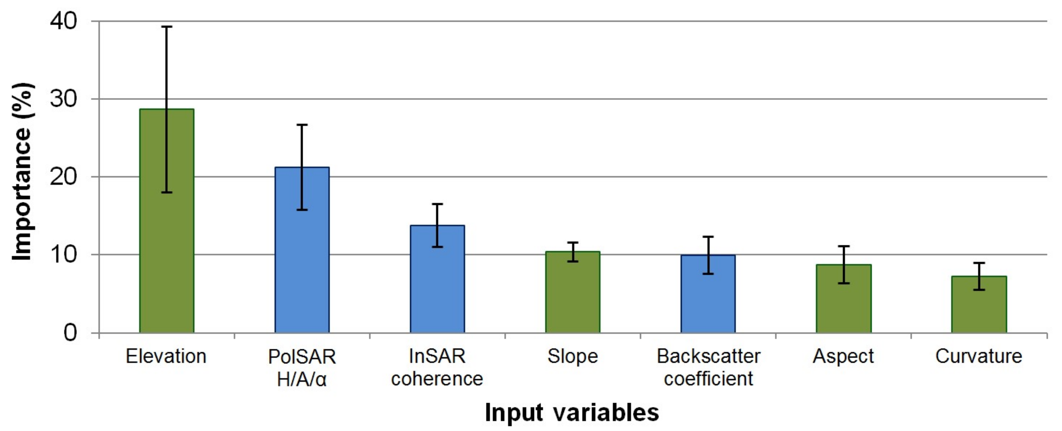
5.1. Influence of Different Input Factors on the Classification Accuracy

As shown in Section 3.2.4, the highest classification accuracy can be obtained when including all three SAR-based observations and all four topographical factors. This finding is not surprising as the influence of the abovementioned parameters has already been reported in previous studies [24,83,84,85,86]. Nevertheless, the impact of these variables has only been evaluated separately. The combination of all parameters in one single approach, as it was implemented for the presented study, turned out to achieve the best results. Topography influences the melting and distribution of snow in mountain regions and was; therefore, included in several approaches to map dry SCE based on wet SCE [17,83,87,88,89]. Hence, its influence on the RF-based approach implemented for the presented study is also significant. Moreover, among all three SAR-based observations and the four topographical parameters, PolSAR and elevation resulted in having the highest impact on the classification accuracy, as illustrated in Figure 4. Comparing the classification accuracy relying on only one SAR-based observation (Figure 4a), PolSAR parameters (P) can generate the highest accuracy comparing to backscattering (B) and InSAR coherence (I). For instance, in the urban land cover type, the accuracy of the B/I/P-based cases is around 0.71, 0.72, and 0.79, respectively. Comparing the accuracy testing with only adding one topographical factor (Figure 4b), elevation shows the most significant improvement as the accuracy of grass land can improve from original 0.71 (using only SAR-based observations) to 0.83 when only adding elevation information, but only enhance to 0.72, 0.73, and 0.76 when adding aspect, curvature, and slope information, respectively. This might be because PolSAR contains much more physical information of the ground conditions, such as characteristics of ground surface, than the relatively noisy backscattering and the InSAR coherence.

The importance of both PolSAR parameters and elevation can also be revealed by the ranks of importance of the variables generated by the RF model. The importance of each input variable of each land cover-targeted RF model was weighted, averaged by the percentage of land cover class for each region. The average importance of each variable for all five study areas is illustrated in Figure 13. Although the importance of the variables in each region is different, it is obvious that for all of the regions, elevation and PolSAR parameters have the highest importance. InSAR coherence also shows considerable contribution to the model accuracy comparing to less important variables such as slope, backscatter, aspect, and curvature. However, due to the fact that: (1) all those input variables were confirmed related to snow cover by previous studies; (2) even the least important variable (i.e., curvature) still has an importance of more than 5%; (3) the importance of each input variable differs for each region; and (4) the goal of the proposed approach is to guarantee global transferability, no input variable was trimmed out in the proposed modeling approach to ensure broader suitability and flexibility.

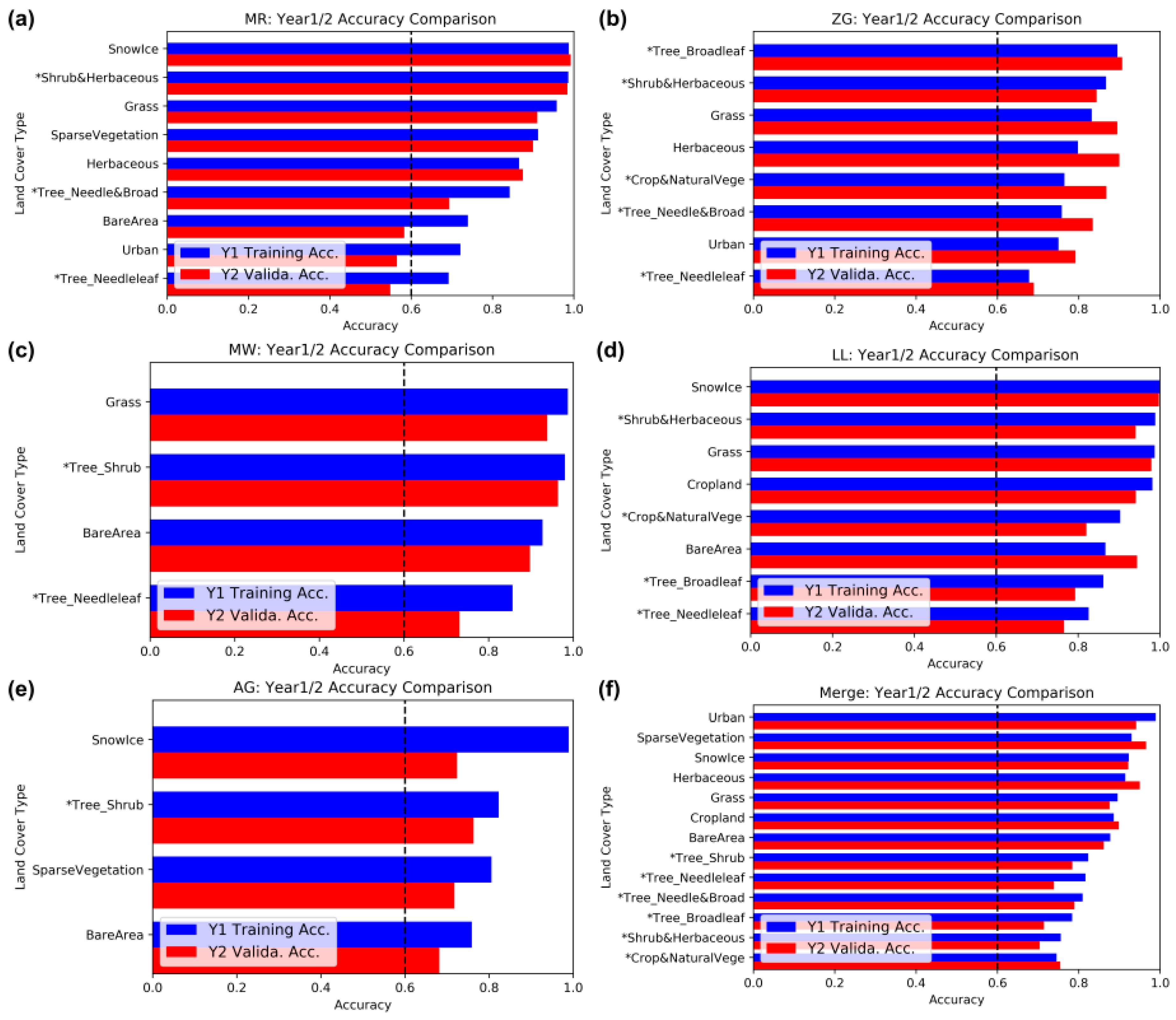
5.2. Influence of Vegetation and Land Cover Types on the Classification Accuracy

The evaluation of the RF performance revealed that the snow cover classification accuracy varies significantly between land cover classes (compare Figure 4, Figure 6 and Figure 7). Densely vegetated regions tend to yield lower SCE accuracy when compared to, for example, bare area, sparse vegetation, urban areas, or even grasslands. These findings match with previous studies’ conclusions: Koskinen et al. [73] stated that the existence of vegetation will greatly reduce the difference between SCE and other land cover features. It has further been confirmed by simulation that the stem volume of forests directly relates to SAR signals [74], which influences land cover classes with even less biomass, such as grassland or cropland [22,90]. Duguay and Bernier [91] found that the vegetation height would impact the SAR backscattering as well. Moreover, Dedieu et al. [47] suggested that the structure and phenological change of trees would also affect how the SAR signal reflects and bounces, as it was also observed by Park et al. [83]. Venkataraman [75] realized that the random motion of vegetation also causes dramatic loss of InSAR coherence.

5.3. Challenges for Validating SAR-Based Snow Cover Classifications; the Case of Aconcagua (AG) Region

After validating the modeled total SCE results, some regions ended up performing better than others. The most apparent example where several factors come into play is the AG test site. The external validation with optical-derived SCE maps (Figure 9) proves the under-estimation of the actual SCE in month1 and the over-estimation in month2. One of the possible reasons is that the land cover product provided by of ESA CCI might be biased for this region. Some of the classes (e.g., scrubland) appear to be overestimated when checked manually, relying on very high-resolution imagery from, for example, Google Earth. Around 57% of the AG region is labeled scrubland in the land cover product. When reviewing the quality flag of the ESA CCI land cover product, a lack of available input data can be constituted. As shown in Figure 14, the AG region’s land cover product is based on considerably less input data than any other region, which might be an indicator that the quality is also poor. In addition to that, according to the ESA CCI land cover product user guidance [39], some specific classes, such as sparse vegetation (which accounts for around 23.5% of the AG region), have relatively low classification accuracies. Considering that the total SCE mapping approach proposed in this study is land cover dependent, possible biases in the land cover product would inevitably reduce the robustness of model. As a result, a significant under- and over-estimation could be connected to this issue. To prove this assumption, we also tested the influence of erroneous land cover classes on the classification accuracy in the Monte Rosa (MR) region. First, land cover class labels were randomly shuffled, and the first year’s model internal validations as well as the second year’s external validation of the resultant SCE were examined (according to Figure 3). A decline of around 3% in overall accuracy was found in the internal cross-validation using first year GSP data, and around 20% and 31% of overestimation were shown in month1/2, validated with optical-based SCE, respectively. Based on this test, it is confirmed that the quality of land cover labelling is important.

The influence of the topographical parameters on the classification performance is equally significant, as outlined in Section 3.2.4 (compare also Figure 4 and Figure 13). Possible errors in the SRTM version 4 DEM could; therefore, also contribute to miss-classifications of SCE. As reported by Rodriguez et al. [92], the SRTM DEM can have absolute height errors of more than 30 m. Since all four topographical parameters are directly derived from the height measurements, biases could cause false model presumptions that would further translate into classification errors.

Finally, the snow cover product (GSP, which is based on MODIS) utilized to train the model could be biased, too. GSP was chosen as an input because it provides daily snow cover information, which is desirable as snowfall events can occur spontaneously. The relatively coarse resolution (500 m), and the fact that clouds can cover large proportions of the study regions, contribute to uncertainties when training the model.

Any of these factors could be responsible for the relatively poor SCE classification accuracy of the AG test region. It is difficult to determine which is the pivotal factor though, as more tests would be required; while also for some input datasets (like SRTM and GSP) no quality flag is available, which quantitatively characterizes the pixel-wise errors.

5.4. Uncertainties of Mapping Wet and Dry SCE in a Holistic Map; the Case of Monte Rosa (MR) Region

As shown in Figure 12b, it is clear that, during the melting season, there is a dry SCE boundary buffering around the wet SCE, especially for the Alpine Monte Rosa region. The possible reasons could include both the over-estimation of our modeled total SCE and the under-estimation of wet SCE detected by “Nagler’s method”.

According to the confusion matrix comparing “modeled” and “optical-based” total SCE, as shown in Figure 9, there is a slight over-estimation observed in month2 of the Monte Rosa region caused by classification error. However, Nagler’s backscattering-based “hard” thresholding approach was also commonly found to under-estimate wet SCE, especially around the snow line where wet snow is patchy [17,93,94,95]. In detail, because snow has a significantly lower scattering cross-section than bare ground, the stronger backscattering signals of bare soil, rock, and vegetation would; thus, dominate that mixed pixel [94,95,96]. This situation mostly can only be compensated by enhancing the spatial resolution of SAR image, as tested by Malnes et al. [96].

5.5. Improvements Achieved in this Study

Although there have been some studies employing machine-learning to classify total SCE, the presented study utilized a novel fusion of multiple SAR-based observations and topographical factors to achieve a higher reliability. The proposed land cover-dependent model has successfully been applied in different study areas. In detail, the improvements when compared to earlier studies can be summarized as follows:

(1). The method provides global suitability and transferability

To achieve a universal, global transferability, the method needs to satisfy both data availability and model robustness. First, for data availability, all datasets being used in this study are available globally. More importantly, all input data are openly accessible, including the spaceborne SAR and optical imagery, the DEM, and the land cover product. Additionally, no field measurements for snow depth, temperature or forest’s stem volume are needed. When it comes to the model’s robustness, most of the previous studies applied the SCE mapping to a single regional site [30,97,98], which implies that they might be site-dependent approaches. In contrast, the presented method is tested in five independent regions located in different mountain ranges and even hemispheres. The achieved accuracy confirms that the proposed method can be applied to map SCE around the globe, which ensures the transferability. Moreover, merging the five regions’ data to build a universal model set, a stable classification accuracy could also be confirmed.

(2). The method can efficiently deal with all land cover types, including forests

Because of challenging SAR-vegetation interactions, many existing studies simply masked out the forest or even agricultural regions [17,18,30,99,100,101,102]. As illustrated in Figure 1, vegetation is a dominant part of land cover in all five study regions. Masking out the vegetation would significantly reduce the suitability of the SCE mapping approach to provide snow cover information for further applications. To overcome this limitation, the presented study includes all land cover types, comprising vegetation-dominated classes such as forest, scrub-, grass-, and crop-land. The model is trained individually for each land cover type to form a land cover-dependent model set. Thanks to the simplicity and robustness of random forest classifiers, they can efficiently process various SAR observations under low computation demands.

(3). The method provides holistic wet and total SCE

Existing methods to detect snow cover from SAR data often focus on wet SCE only. The presented study proposes a method to derive both wet and total SCE, relying on a combination of an RF-based classifier to map the total SCE and a backscattering-based approach to detect wet SCE (Nagler’s method). Thanks to the performance of the RF classifier, the workflow offers an option for near real-time and automatic classification of wet and dry SCE, thus enhancing the viability of spaceborne SAR data to map SCE. Since the method provides both wet and dry SCE, it could offer new ways of how remote sensing-based snow cover products can be incorporated into hydrological models.

5.6. Future Work

Considering the PolSAR data, existing studies have demonstrated that quad-polarization imagery can provide more satisfying results than dual-polarization, as it can reduce topographical distortions [46] and is also more sensitive to the state of snow [47]. Thus, the potential of utilizing the TerraSAR-X or Radarsat-2 should be explored. Moreover, their ultra-high-resolution sensing mode can also enhance the accuracy of wet SCE mapping as discussed in Section 5.4.

Regarding the auxiliary data, one of the future developments to improve the classification accuracy in vegetated areas will include the use of quantitative vegetation measurements, such as biomass density, the normalized difference vegetation index, or the leaf area index. The local incidence angle (LIA) of the SAR imagery related to the local topography may also be included to justify the impact of topography.

6. Conclusions

There are many studies available for detecting wet snow cover extent (SCE) utilizing spaceborne SAR imagery. However, there exists no properly-validated, globally transferable, total SCE mapping approach that would be applicable to all land cover classes. The presented study proposed a novel approach to map total and wet SCE based on openly accessible datasets (including SAR imagery, DEM, and land cover product) with global coverage. Thanks to the simplicity and efficiency of the implemented random forest classifier, it is possible to incorporate non-linear and complex SAR-based observations (InSAR, PolSAR, backscattering). In regards to the influence of topography, four topographical factors, including elevation, slope, aspect, and curvature, were also included as model inputs. The method has been applied to different mountainous locations (five regions located in different mountain ranges, continents, and hemispheres) over a period of different months and years. By extending the RF-based classification with a backscattering-based thresholding approach, information about wet SCE was additionally supplemented. Internal as well as external independent validation have been comprehensively conducted, confirming the robustness and transferability of the proposed method.

In addition to the global transferability, another merit of the presented approach is the capability to detect snow cover in vegetated areas, such as forests, grass-, scrub-, and crop-lands. Compared to previous studies, which often masked out the forest or even agricultural regions, this study proposed a land cover-dependent classification procedure to solve this limitation. Namely, total SCE was classified with SAR observations and topographical factors in each land cover class separately, before merging each classes’ model to form a universal model set. To explore the influence of all inputs, the accuracy of each model set, built by different combinations of SAR observations and topographical factors, was evaluated. Results prove that the model set including all three SAR-based observations (InSAR, PolSAR, backscattering) as well as all four topographical factors (elevation, slope, aspect, curvature) yields the highest classification accuracy for all land cover types. Overall accuracy, F-measure, and AUC score can reach around 80%, 80%, and 70% for the majority of the regions. The accuracy can even be higher, around 5%, if vegetation land cover classes are excluded. It was also found that PolSAR and elevation provide more information than the remaining parameters. Additionally, when merging all input data for all test sites into one universal, general model (i.e., building a universally applicable model set), the accuracy remains satisfying. Future developments will include the incorporation of quantitative vegetation parameters (leaf area index, biomass, normalized difference vegetation index) as well as the local incidence angle of the SAR observations.

References

1. Kevin, J.-P.W.; Kotlarski, S.; Scherrer, S.C.; Schär, C. The Alpine snow-albedo feedback in regional climate models. Clim. Dyn. 2017, 48, 1109–1124. [Google Scholar]
2. Huss, M.; Bookhagen, B.; Huggel, C.; Jacobsen, D.; Bradley, R.S.; Clague, J.J.; Vuille, M.; Buytaert, W.; Cayan, D.R.; Greenwood, G. Toward mountains without permanent snow and ice. Earth’s Future 2017, 5, 418–435. [Google Scholar] [CrossRef]
3. Ancey, C.; Bain, V. Dynamics of glide avalanches and snow gliding. Rev. Geophys. 2015, 53, 745–784. [Google Scholar] [CrossRef]
4. Dorji, T.; Hopping, K.A.; Wang, S.; Piao, S.; Tarchen, T.; Klein, J.A. Grazing and spring snow counteract the effects of warming on an alpine plant community in Tibet through effects on the dominant species. Agric. For. Meteorol. 2018, 263, 188–197. [Google Scholar] [CrossRef]
5. Beniston, M.; Farinotti, D.; Stoffel, M.; Andreassen, L.M.; Coppola, E.; Eckert, N.; Fantini, A.; Giacona, F.; Hauck, C.; Huss, M. The European mountain cryosphere: A review of its current state, trends, and future challenges. Cryosphere 2018, 12, 759–794. [Google Scholar] [CrossRef]
6. Bulygina, O.; Razuvaev, V.; Korshunova, N. Changes in snow cover over Northern Eurasia in the last few decades. Environ. Res. Lett. 2009, 4, 045026. [Google Scholar] [CrossRef]
7. Brown, R.D.; Robinson, D.A. Northern Hemisphere spring snow cover variability and change over 1922–2010 including an assessment of uncertainty. Cryosphere 2011, 5, 219–229. [Google Scholar] [CrossRef]
8. Dyrrdal, A.V.; Saloranta, T.; Skaugen, T.; Stranden, H.B. Changes in snow depth in Norway during the period 1961–2010. Hydrol. Res. 2013, 44, 169–179. [Google Scholar] [CrossRef]
9. Pachauri, R.K.; Allen, M.R.; Barros, V.R.; Broome, J.; Cramer, W.; Christ, R.; Church, J.A.; Clarke, L.; Dahe, Q.; Dasgupta, P. Climate Change 2014: Synthesis Report. Contribution of Working Groups I, II and III to the Fifth Assessment Report of the Intergovernmental Panel on Climate Change; IPCC: Geneva, Switzerland, 2014. [Google Scholar]
10. Hoegh-Guldberg, O.; Jacob, D.; Taylor, M.; Bindi, M.; Brown, S.; Camilloni, I.; Diedhiou, A.; Djalante, R.; Ebi, K.; Engelbrecht, F. Impacts of 1.5 °C Global Warming on Natural and Human Systems; IPCC: Geneva, Switzerland, 2018. [Google Scholar]
11. Schmucki, E.; Marty, C.; Fierz, C.; Lehning, M. Simulations of 21st century snow response to climate change in Switzerland from a set of RCMs. Int. J. Climatol. 2015, 35, 3262–3273. [Google Scholar] [CrossRef]
12. Riggs, G.A.; Hall, D.K. MODIS Snow Products Collection 6 User Guide; National Snow and Ice Data Center: Boulder, CO, USA, 2015. [Google Scholar]
13. Solberg, R.; Wangensteen, B.; Metsämäki, S.; Nagler, T.; Sandner, R.; Rott, H.; Wiesmann, A.; Luojus, K.; Kangwa, M.; Pulliainen, J. GlobSnow Snow Extent Product Guide Product, version 1.0; European Space Agency: Espoo, Finland, 2010. [Google Scholar]
14. Dietz, A.J.; Kuenzer, C.; Dech, S. Global SnowPack: A new set of snow cover parameters for studying status and dynamics of the planetary snow cover extent. Remote Sens. Lett. 2015, 6, 844–853. [Google Scholar] [CrossRef]
15. Metsämäki, S.; Ripper, E.; Mattila, O.-P.; Fernandes, R.; Schwaizer, G.; Luojus, K.; Nagler, T.; Bojkov, B.; Kern, M. Evaluation of Northern Hemisphere and regional snow extent products within ESA SnowPEx-project. In Proceedings of the 2017 IEEE International Geoscience and Remote Sensing Symposium (IGARSS), Fort Worth, TX, USA, 23–28 July 2017; pp. 4246–4249. [Google Scholar]
16. Macander, M.J.; Swingley, C.S.; Joly, K.; Raynolds, M.K. Landsat-based snow persistence map for northwest Alaska. Remote Sens. Environ. 2015, 163, 23–31. [Google Scholar] [CrossRef]
17. Nagler, T.; Rott, H. Retrieval of wet snow by means of multitemporal SAR data. IEEE Trans. Geosci. Remote Sens. 2000, 38, 754–765. [Google Scholar] [CrossRef]
18. Notarnicola, C.; Ratti, R.; Maddalena, V.; Schellenberger, T.; Ventura, B.; Zebisch, M. Seasonal Snow Cover Mapping in Alpine Areas Through Time Series of COSMO-SkyMed Images. IEEE Geosci. Remote Sens. Lett. 2013, 10, 716–720. [Google Scholar] [CrossRef]
19. Salcedo, A.P.; Cogliati, M.G. Snow Cover Area Estimation Using Radar and Optical Satellite Information. Atmos. Clim. Sci. 2014, 04, 514–523. [Google Scholar] [CrossRef]
20. Luojus, K.P.; Pulliainen, J.T.; Metsamaki, S.J.; Hallikainen, M.T. Accuracy assessment of SAR data-based snow-covered area estimation method. IEEE Trans. Geosci. Remote Sens. 2006, 44, 277–287. [Google Scholar] [CrossRef]
21. Venkataraman, G.; Singh, G.; Kumar, V. Snow cover area monitoring using multi-temporal TerraSAR-X data. In Proceedings of the Third TerraSAR-X Science Team Meeting, DLR, Cologne, Germany, 17–20 October 2016. [Google Scholar]
22. Schellenberger, T.; Ventura, B.; Zebisch, M.; Notarnicola, C. Wet Snow Cover Mapping Algorithm Based on Multitemporal COSMO-SkyMed X-Band SAR Images. IEEE J. Sel. Top. Appl. Earth Obs. Remote Sens. 2012, 5, 1045–1053. [Google Scholar] [CrossRef]
23. Magagi, R.; Bernier, M. Optimal conditions for wet snow detection using RADARSAT SAR data. Remote Sens. Environ. 2003, 84, 221–233. [Google Scholar] [CrossRef]
24. Nagler, T.; Rott, H.; Ripper, E.; Bippus, G.; Hetzenecker, M. Advancements for snowmelt monitoring by means of sentinel-1 SAR. Remote Sens. 2016, 8, 348. [Google Scholar] [CrossRef]
25. Snehmani; Singh, M.K.; Gupta, R.D.; Bhardwaj, A.; Joshi, P.K. Remote sensing of mountain snow using active microwave sensors: A review. GeoCart Intern. 2015, 30, 1–27. [Google Scholar] [CrossRef]
26. Singh, G.; Venkataraman, G.; Rao, Y.S.; Kumar, V. InSAR coherence measurement techniques for snow cover mapping in Himalayan region. In Proceedings of the IEEE International Geoscience and Remote Sensing Symposium, IGARSS 2008, Boston, MA, USA, 7–11 July 2008; pp. IV-1077–IV-1080. [Google Scholar]
27. Cloude, S.R.; Pottier, E. A review of target decomposition theorems in radar polarimetry. IEEE Trans. Geosci. Remote Sens. 1996, 34, 498–518. [Google Scholar] [CrossRef]
28. Huang, L.; Li, Z.; Tian, B.-S.; Chen, Q.; Liu, J.-L.; Zhang, R. Classification and snow line detection for glacial areas using the polarimetric SAR image. Remote Sens. Environ. 2011, 115, 1721–1732. [Google Scholar] [CrossRef]
29. Longepe, N.; Shimada, M.; Allain, S.; Pottier, E. Capabilities of full-polarimetric PALSAR/ALOS for snow extent mapping. In Proceedings of the IEEE International Geoscience and Remote Sensing Symposium, IGARSS 2008, Boston, MA, USA, 7–11 July 2008; pp. IV-1026–IV-1029. [Google Scholar]
30. He, G.; Feng, X.; Xiao, P.; Xia, Z.; Wang, Z.; Chen, H.; Li, H.; Guo, J. Dry and Wet Snow Cover Mapping in Mountain Areas Using SAR and Optical Remote Sensing Data. IEEE J. Sel. Top. Appl. Earth Obs. Remote Sens. 2017, 10, 2575–2588. [Google Scholar] [CrossRef]
31. Usami, N.; Muhuri, A.; Bhattacharya, A.; Hirose, A. PolSAR wet snow mapping with incidence angle information. IEEE Geosci. Remote Sens. Lett. 2016, 13, 2029–2033. [Google Scholar] [CrossRef]
32. Pal, M. Random forest classifier for remote sensing classification. Int. J. Remote Sens. 2005, 26, 217–222. [Google Scholar] [CrossRef]
33. Adam, E.; Mutanga, O.; Odindi, J.; Abdel-Rahman, E.M. Land-use/cover classification in a heterogeneous coastal landscape using RapidEye imagery: Evaluating the performance of random forest and support vector machines classifiers. Int. J. Remote Sens. 2014, 35, 3440–3458. [Google Scholar] [CrossRef]
34. Rodriguez-Galiano, V.; Sanchez-Castillo, M.; Chica-Olmo, M.; Chica-Rivas, M. Machine learning predictive models for mineral prospectivity: An evaluation of neural networks, random forest, regression trees and support vector machines. Ore Geol. Rev. 2015, 71, 804–818. [Google Scholar] [CrossRef]
35. Jarvis, A.; Reuter, H.I.; Nelson, A.; Guevara, E. Hole-Filled SRTM for the Globe, version 4; CGIAR Consortium for Spatial Information: Washington, DC, USA, 2008. [Google Scholar]
36. Frey, H.; Paul, F. On the suitability of the SRTM DEM and ASTER GDEM for the compilation of topographic parameters in glacier inventories. Int. J. Appl. Earth Obs. Geoinf. 2012, 18, 480–490. [Google Scholar] [CrossRef]
37. Hirt, C.; Filmer, M.; Featherstone, W. Comparison and validation of the recent freely available ASTER-GDEM ver1, SRTM ver4. 1 and GEODATA DEM-9S ver3 digital elevation models over Australia. Aust. J. Earth Sci. 2010, 57, 337–347. [Google Scholar] [CrossRef]
38. Athmania, D.; Achour, H. External Validation of the ASTER GDEM2, GMTED2010 and CGIAR-CSI- SRTM v4.1 Free Access Digital Elevation Models (DEMs) in Tunisia and Algeria. Remote Sens. 2014, 6, 4600. [Google Scholar] [CrossRef]
39. ESA. Land Cover CCI Product User Guide, version 2.0; CCI-LC-PUGV2; 2017. Available online: https://www.esa-landcover-cci.org/?q=webfm_send/84 (accessed on 10 April 2019).
40. Lee, J.-S. Digital image smoothing and the sigma filter. Comput. Vis. Graph. Image Process. 1983, 24, 255–269. [Google Scholar] [CrossRef]
41. Lavalle, M.; Wright, T. Absolute Radiometric and polarimetric Calibration of ALOS PALSAR Products, Document Issue (1), Revision (3); Scientific Research Publishing Inc.: Wuhan, China, 2009.
42. Zebker, H.A.; Villasenor, J. Decorrelation in interferometric radar echoes. IEEE Trans. Geosci. Remote Sens. 1992, 30, 950–959. [Google Scholar] [CrossRef]
43. Lee, J.-S.; Pottier, E. Polarimetric Radar Imaging: From Basics to Applications; CRC Press: Boca Raton, FL, USA, 2009. [Google Scholar]
44. Pellizzeri, T.M. Classification of polarimetric SAR images of suburban areas using joint annealed segmentation and “H/A/α” polarimetric decomposition. ISPRS J. Photogramm. Remote Sens. 2003, 58, 55–70. [Google Scholar] [CrossRef]
45. Lee, J.-S. Refined filtering of image noise using local statistics. Comput. Vis. Graph. Image Process. 1981, 15, 380–389. [Google Scholar] [CrossRef]
46. Singh, G.; Venkataraman, G.; Yamaguchi, Y.; Park, S.-E. Capability Assessment of Fully Polarimetric ALOS–PALSAR Data for Discriminating Wet Snow From Other Scattering Types in Mountainous Regions. IEEE Trans. Geosci. Remote Sens. 2014, 52, 1177–1196. [Google Scholar] [CrossRef]
47. Dedieu, J.-P.; De Farias, G.B.; Castaings, T.; Allain-Bailhache, S.; Pottier, E.; Durand, Y.; Bernier, M. Interpretation of a RADARSAT-2 fully polarimetric time-series for snow cover studies in an Alpine context–first results. Can. J. Remote Sens. 2012, 38, 336–351. [Google Scholar] [CrossRef]
48. Callegari, M.; Carturan, L.; Marin, C.; Notarnicola, C.; Rastner, P.; Seppi, R.; Zucca, F. A Pol-SAR Analysis for Alpine Glacier Classification and Snowline Altitude Retrieval. IEEE J. Sel. Top. Appl. Earth Obs. Remote Sens. 2016, 9, 3106–3121. [Google Scholar] [CrossRef]
49. Singh, G.; Venkataraman, G. Application of incoherent target decomposition theorems to classify snow cover over the Himalayan region. Int. J. Remote Sens. 2012, 33, 4161–4177. [Google Scholar] [CrossRef]
50. Key, J.; Drinkwater, M.; Ukita, J. IGOS Cryosphere Theme Report; WMO/TD-No. 1405; World Meteorological Organization: Geneva, Switzerland, 2007; 100p. [Google Scholar]
51. Breiman, L. Random forests. Mach. Learn. 2001, 45, 5–32. [Google Scholar] [CrossRef]
52. Archer, K.J.; Kimes, R.V. Empirical characterization of random forest variable importance measures. Comput. Stat. Data Anal. 2008, 52, 2249–2260. [Google Scholar] [CrossRef]
53. Sazonau, V. Implementation and Evaluation of a Random Forest Machine Learning Algorithm; University of Manchester: Manchester, UK, 2012. [Google Scholar]
54. Horning, N. Introduction to Decision Trees and Random Forests; American Museum of Natural History: New York, NY, USA, 2013. [Google Scholar]
55. Ali, J.; Khan, R.; Ahmad, N.; Maqsood, I. Random forests and decision trees. Int. J. Comput. Sci. Issues 2012, 9, 272. [Google Scholar]
56. Gislason, P.O.; Benediktsson, J.A.; Sveinsson, J.R. Random Forests for land cover classification. Pattern Recognit. Lett. 2006, 27, 294–300. [Google Scholar] [CrossRef]
57. Belgiu, M.; Drăguţ, L. Random forest in remote sensing: A review of applications and future directions. ISPRS J. Photogramm. Remote Sens. 2016, 114, 24–31. [Google Scholar] [CrossRef]
58. Cutler, D.R.; Edwards, T.C., Jr.; Beard, K.H.; Cutler, A.; Hess, K.T.; Gibson, J.; Lawler, J.J. Random forests for classification in ecology. Ecology 2007, 88, 2783–2792. [Google Scholar] [CrossRef] [PubMed]
59. Rodriguez-Galiano, V.F.; Chica-Olmo, M.; Abarca-Hernandez, F.; Atkinson, P.M.; Jeganathan, C. Random Forest classification of Mediterranean land cover using multi-seasonal imagery and multi-seasonal texture. Remote Sens. Environ. 2012, 121, 93–107. [Google Scholar] [CrossRef]
60. Ham, J.; Chen, Y.; Crawford, M.M.; Ghosh, J. Investigation of the random forest framework for classification of hyperspectral data. IEEE Trans. Geosci. Remote Sens. 2005, 43, 492–501. [Google Scholar] [CrossRef]
61. Chan, J.C.-W.; Paelinckx, D. Evaluation of Random Forest and Adaboost tree-based ensemble classification and spectral band selection for ecotope mapping using airborne hyperspectral imagery. Remote Sens. Environ. 2008, 112, 2999–3011. [Google Scholar] [CrossRef]
62. Immitzer, M.; Atzberger, C.; Koukal, T. Tree Species Classification with Random Forest Using Very High Spatial Resolution 8-Band WorldView-2 Satellite Data. Remote Sens. 2012, 4, 2661–2693. [Google Scholar] [CrossRef]
63. Immitzer, M.; Vuolo, F.; Atzberger, C. First Experience with Sentinel-2 Data for Crop and Tree Species Classifications in Central Europe. Remote Sens. 2016, 8, 166. [Google Scholar] [CrossRef]
64. Feng, Q.; Liu, J.; Gong, J. UAV Remote Sensing for Urban Vegetation Mapping Using Random Forest and Texture Analysis. Remote Sens. 2015, 7, 1074. [Google Scholar] [CrossRef]
65. Ghosh, A.; Fassnacht, F.E.; Joshi, P.; Koch, B. A framework for mapping tree species combining hyperspectral and LiDAR data: Role of selected classifiers and sensor across three spatial scales. Int. J. Appl. Earth Obs. Geoinf. 2014, 26, 49–63. [Google Scholar] [CrossRef]
66. Du, P.; Samat, A.; Waske, B.; Liu, S.; Li, Z. Random forest and rotation forest for fully polarized SAR image classification using polarimetric and spatial features. ISPRS J. Photogramm. Remote Sens. 2015, 105, 38–53. [Google Scholar] [CrossRef]
67. Cánovas-García, F.; Alonso-Sarría, F.; Gomariz-Castillo, F.; Oñate-Valdivieso, F. Modification of the random forest algorithm to avoid statistical dependence problems when classifying remote sensing imagery. Comput. Geosci. 2017, 103, 1–11. [Google Scholar] [CrossRef]
68. Canovas-Garcia, F.; Alonso-Sarria, F. Optimal combination of classification algorithms and feature ranking methods for object-based classification of submeter resolution Z/I-Imaging DMC imagery. Remote Sens. 2015, 7, 4651–4677. [Google Scholar] [CrossRef]
69. Lewis, D.D.; Gale, W.A. A sequential algorithm for training text classifiers. In Proceedings of the 17th Annual International ACM SIGIR Conference on Research and Development in Information Retrieval, Dublin, Ireland, 3–6 July 1994; pp. 3–12. [Google Scholar]
70. Fawcett, T. An introduction to ROC analysis. Pattern Recognit. Lett. 2006, 27, 861–874. [Google Scholar] [CrossRef]
71. Sokolova, M.; Japkowicz, N.; Szpakowicz, S. Beyond accuracy, F-score and ROC: A family of discriminant measures for performance evaluation. In Proceedings of the Australasian Joint Conference on Artificial Intelligence, Hobart, TAS, Australia, 4–8 December 2006; pp. 1015–1021. [Google Scholar]
72. Ferri, C.; Hernández-Orallo, J.; Modroiu, R. An experimental comparison of performance measures for classification. Pattern Recognit. Lett. 2009, 30, 27–38. [Google Scholar] [CrossRef]
73. Koskinen, J.T.; Pulliainen, J.T.; Hallikainen, M.T. The use of ERS-1 SAR data in snow melt monitoring. IEEE Trans. Geosci. Remote Sens. 1997, 35, 601–610. [Google Scholar] [CrossRef]
74. Pulliainen, J.T.; Heiska, K.; Hyyppa, J.; Hallikainen, M.T. Backscattering properties of boreal forests at the C-and X-bands. IEEE Trans. Geosci. Remote Sens. 1994, 32, 1041–1050. [Google Scholar] [CrossRef]
75. Kumar, V.; Venkataraman, G. SAR interferometric coherence analysis for snow cover mapping in the western Himalayan region. Int. J. Digit. Earth 2011, 4, 78–90. [Google Scholar] [CrossRef]
76. Metz, C.E. Basic principles of ROC analysis. Semin. Nucl. Med. 1978, 8, 283–298. [Google Scholar] [CrossRef]
77. Qiu, S.; He, B.; Zhu, Z.; Liao, Z.; Quan, X. Improving Fmask cloud and cloud shadow detection in mountainous area for Landsats 4–8 images. Remote Sens. Environ. 2017, 199, 107–119. [Google Scholar] [CrossRef]
78. Nagare, M.; Aoki, H.; Kaneko, E. A unified method of cloud detection and removal robust to spectral variability. In Proceedings of the 2017 IEEE International Geoscience and Remote Sensing Symposium (IGARSS), Fort Worth, TX, USA, 23–28 July 2017; pp. 5418–5421. [Google Scholar]
79. Selkowitz, D.; Forster, R. An automated approach for mapping persistent ice and snow cover over high latitude regions. Remote Sens. 2016, 8, 16. [Google Scholar] [CrossRef]
80. Tank, A.K.; Wijngaard, J.; Können, G.; Böhm, R.; Demarée, G.; Gocheva, A.; Mileta, M.; Pashiardis, S.; Hejkrlik, L.; Kern-Hansen, C. Daily dataset of 20th-century surface air temperature and precipitation series for the European Climate Assessment. Int. J. Climatol. 2002, 22, 1441–1453. [Google Scholar] [CrossRef]
81. Hall, D.K.; Riggs, G.A.; Salomonson, V.V.; DiGirolamo, N.E.; Bayr, K.J. MODIS snow-cover products. Remote Sens. Environ. 2002, 83, 181–194. [Google Scholar] [CrossRef]
82. Che, T.; Li, X.; Jin, R.; Armstrong, R.; Zhang, T. Snow depth derived from passive microwave remote-sensing data in China. Ann. Glaciol. 2008, 49, 145–154. [Google Scholar] [CrossRef]
83. Park, S.-E.; Yamaguchi, Y.; Singh, G.; Yamaguchi, S.; Whitaker, A.C. Polarimetric SAR Response of Snow-Covered Area Observed by Multi-Temporal ALOS PALSAR Fully Polarimetric Mode. IEEE Trans. Geosci. Remote Sens. 2014, 52, 329–340. [Google Scholar] [CrossRef]
84. Strozzi, T.; Wegmuller, U.; Matzler, C. Mapping wet snowcovers with SAR interferometry. Int. J. Remote Sens. 1999, 20, 2395–2403. [Google Scholar] [CrossRef]
85. Guo, C.; Tong, L.; Chen, Y.; Yang, X. Snow extraction using X-band multi-temporal coherence based on insar technology. In Proceedings of the 2017 IEEE International Geoscience and Remote Sensing Symposium (IGARSS), Fort Worth, TX, USA, 23–28 July 2017. [Google Scholar]
86. Zhou, C.; Zheng, L. Mapping Radar Glacier Zones and Dry Snow Line in the Antarctic Peninsula Using Sentinel-1 Images. Remote Sens. 2017, 9, 1171. [Google Scholar] [CrossRef]
87. Thakur, P.K.; Aggarwal, S.P.; Arun, G.; Sood, S.; Senthil Kumar, A.; Mani, S.; Dobhal, D.P. Estimation of Snow Cover Area, Snow Physical Properties and Glacier Classification in Parts of Western Himalayas Using C-Band SAR Data. J. Indian Soc. Remote Sens. 2016, 45, 525–539. [Google Scholar] [CrossRef]
88. Malnes, E.; Storvold, R.; Lauknes, I. Near real time snow covered area mapping with Envisat ASAR wideswath in Norwegian mountainous areas. In Proceedings of the ESA ENVISAT & ERS Symposium, Salzburg, Austria, 6–10 September 2004; pp. 6–10. [Google Scholar]
89. Zhen, L.; Lei, H.; Quan, C.; Bang-sen, T. Glacier Snow Line Detection on a Polarimetric SAR Image. IEEE Geosci. Remote Sens. Lett. 2012, 9, 584–588. [Google Scholar] [CrossRef]
90. Löw, A.; Ludwig, R.; Mauser, W. Land use dependent snow cover retrieval using multitemporal, multisensoral SAR-images to drive operational flood forecasting models. In Proceedings of the EARSeL-LISSIG-Workshop Observing our Cryosphere from Space, Bern, Switzerland, 11–13 March 2002. [Google Scholar]
91. Duguay, Y.; Bernier, M. The use of RADARSAT-2 and TerraSAR-X data for the evaluation of snow characteristics in subarctic regions. In Proceedings of the 2012 IEEE International Geoscience and Remote Sensing Symposium (IGARSS), Munich, Germany, 22–27 July 2012; pp. 3556–3559. [Google Scholar]
92. Rodriguez, E.; Morris, C.S.; Belz, J.E. A global assessment of the SRTM performance. Photogramm. Eng. Remote Sens. 2006, 72, 249–260. [Google Scholar] [CrossRef]
93. Malnes, E.; Guneriussen, T. Mapping of snow covered area with Radarsat in Norway. In Proceedings of the 2002 IEEE International Geoscience and Remote Sensing Symposium, IGARSS’02, Toronto, ON, Canada, 24–28 June 2002; pp. 683–685. [Google Scholar]
94. Pettinato, S.; Malnes, E.; Haarpaintner, J. Snow cover maps with satellite borne SAR: A new approach in harmony with fractional optical SCA retrieval algorithms. In Proceedings of the IEEE International Geoscience and Remote Sensing Symposium, IGARSS 2006, Denver, CO, USA, 31 July–4 August 2006; pp. 735–738. [Google Scholar]
95. Storvold, R.; Malnes, E.; Larsen, Y.; Høgda, K.; Hamran, S.; Mueller, K.; Langley, K. SAR remote sensing of snow parameters in norwegian areas—Current status and future perspective. J. Electromagn. Waves Appl. 2006, 20, 1751–1759. [Google Scholar] [CrossRef]
96. Malnes, E.; Storvold, R.; Lauknes, I.; Pettinato, S. Multi-polarisation measurements of snow signatures with air-and satelliteborne SAR. EARSeL eProc. 2006, 5, 111–119. [Google Scholar]
97. Luojus, K.P.; Pulliainen, J.T.; Blasco Cutrona, A.; Metsamaki, S.J.; Hallikainen, M.T. Comparison of SAR-Based Snow-Covered Area Estimation Methods for the Boreal Forest Zone. IEEE Geosci. Remote Sens. Lett. 2009, 6, 403–407. [Google Scholar] [CrossRef]
98. Muhuri, A.; Manickam, S.; Bhattacharya, A.; Snehmani. Snow Cover Mapping Using Polarization Fraction Variation With Temporal RADARSAT-2 C-Band Full-Polarimetric SAR Data Over the Indian Himalayas. IEEE J. Sel. Top. Appl. Earth Obs. Remote Sens. 2018, 1–18. [Google Scholar] [CrossRef]
99. Rott, H.; Nagler, T. Monitoring temporal dynamics of snowmelt with ERS-1 SAR. In Proceedings of the International Geoscience and Remote Sensing Symposium, IGARSS’95, Quantitative Remote Sensing for Science and Applications, Firenze, Italy, 10–14 July 1995; pp. 1747–1749. [Google Scholar]
100. Guangjun, H.; Pengfeng, X.; Xuezhi, F.; Xueliang, Z.; Zuo, W.; Ni, C. Extracting Snow Cover in Mountain Areas Based on SAR and Optical Data. IEEE Geosci. Remote Sens. Lett. 2015, 12, 1136–1140. [Google Scholar] [CrossRef]
101. Luojus, K.P.; Pulliainen, J.T.; Metsamaki, S.J.; Hallikainen, M.T. Snow-Covered Area Estimation Using Satellite Radar Wide-Swath Images. IEEE Trans. Geosci. Remote Sens. 2007, 45, 978–989. [Google Scholar] [CrossRef]
102. Wang, Y.; Wang, L.; Li, H.; Yang, Y.; Yang, T. Assessment of Snow Status Changes Using L-HH Temporal-Coherence Components at Mt. Dagu, China. Remote Sens. 2015, 7, 11602–11620. [Google Scholar] [CrossRef]
Figure 1. Land cover types (derived from European Space Agency (ESA) Climate Change Initiative (CCI) land cover product) for the five selected test sites: (a) Monte Rosa (MR), (b) Zugspitze (ZG), (c) Mount Whitney (MW), (d) Landtang Lirung (LL), and (e) Aconcagua (AG). Location of each region around the globe is illustrated in (f).
Remotesensing 11 00895 g001
Figure 2. Selected date of synthetic aperture radar (SAR) imagery for five regions in two hydrological years. The seasonal cycle of snow cover extent (SCE) is illustrated as a blue curve.
Remotesensing 11 00895 g002
Figure 3. Data splitting for model training and validation including internal validation, external validation, out-of-bag (OOB) sample, and training sample based on Global SnowPack (GSP), optical-based snow cover extent (SCE), and snow depth data.
Remotesensing 11 00895 g003
Figure 4. Assessment of the influence of different input combinations on the performance of the model for Monte Rosa (MR) region. SAR-based observations including backscattering ratio, interferometric SAR (InSAR) coherence, and polarimetric (PolSAR) H/A/α parameters are abbreviated as B, I, and P, respectively. Topographical factors including aspect, slope, curvature, and elevation are abbreviated as a, s, c, and e, respectively. Accuracy of each land cover type modeled with SAR-based observations only or together with topographical factors is shown in (a) and (b), respectively. Non-forest classes’ overall accuracy, F measure, and area under the receiver operating characteristic curve are abbreviated as NF OA, NF F1, and NF AUC, respectively.
Remotesensing 11 00895 g004
Figure 5. Overall workflow of mapping and validating holistic (total + wet) Snow Cover Extent (SCE) with SAR-based observations, topographical information, land cover information, and Global SnowPack (GSP) daily snow cover information. Single look complex, ground range detected, shuttle radar topographic mission digital elevation model, and land cover are abbreviated as SLC, GRD, SRTM DEM, and LC, respectively.
Remotesensing 11 00895 g005
Figure 6. Results of each model set built in each region: (a) Monte Rosa (MR), (b) Zugspitze (ZG), (c) Mount Whitney (MW), (d) Landtang Lirung (LL), and (e) Aconcagua (AG); and the five regions’ merging case (f). SAR-based observations including backscattering ratio, InSAR coherence, and PolSAR H/A/α parameters are abbreviated as B, I, and P, respectively. Topographical factors including aspect, slope, curvature, and elevation are abbreviated as a, s, c, and e, respectively.
Remotesensing 11 00895 g006
Figure 7. Each region’s land cover types’ accuracy comparison between training (first hydrological year) and validation set (second hydrological year). Model built for each region: (a) Monte Rosa (MR), (b) Zugspitze (ZG), (c) Mount Whitney (MW), (d) Landtang Lirung (LL), and (e) Aconcagua (AG); and the five regions’ merging case (f).
Remotesensing 11 00895 g007
Figure 8. Fmask-based total snow cover extent classification derived from Landsat and Sentinel-2 as well as true-color composites for each test site: (a) Monte Rosa (MR), month 1 (23 March 2018); (b) Monte Rosa, month 2 (18 May 2018); (c) Zugspitze (ZG), month 1 (25 March 2018); (d) Zugspitze, month 2 (07 May 2018); (e) Mount Whitney (MW), month 1 (16 March 2018); (f) Mount Whitney, month 2 (03 May 2018); (g) Landtang Lirung (LL), month 1 (13 March 2018); (h) Landtang Lirung, month 2 (16 May 2018); (i) Aconcagua (AG), month 1 (13 June 2018); (j) Aconcagua, month 2 (04 May 2018).
Remotesensing 11 00895 g008
Figure 9. Confusion matrix of the accuracy assessment relying on optical-based snow cover classifications of Landsat and Sentinel-2 for each test site. The assessment includes classifications for months that were trained in the first year (month2) as well as those that were not used in the training of the first year (month1). Overall accuracy (OA) and F1-score are depicted under the respective confusion matrix.
Remotesensing 11 00895 g009
Figure 10. Location of meteorological stations in Monte Rosa (MR) and Zugspitze (ZG) regions.
Remotesensing 11 00895 g010
Figure 11. (A): Confusion matrix of Monte Rosa (MR) and (B) Zugspitze (ZG) regions validated with meteorological snow depth (SD) station data records of MeteoSwiss and European Climate Assessment and Dataset Project (ECA&D), respectively.
Remotesensing 11 00895 g011
Figure 12. Total and wet snow cover extent (SCE) of each regions’ two months: (a) Monte Rosa (MR), month 1 (12 March 2018); (b) Monte Rosa, month 2 (11 May 2018); (c) Zugspitze (ZG), month 1 (14 March 2018); (d) Zugspitze, month 2 (13 May 2018); (e) Mount Whitney (MW), month 1 (04 March 2018); (f) Mount Whitney, month 2 (03 May 2018); (g) Landtang Lirung (LL), month 1 (28 February 2018); (h) Landtang Lirung, month 2 (11 May 2018); (i) Aconcagua (AG), month 1 (10 June 2018); (j) Aconcagua, month 2 (05 May 2018).
Remotesensing 11 00895 g012
Figure 13. The average importance of input variables for all five study regions. Blue and green bars represent SAR-based observations and topographical factors, respectively.
Remotesensing 11 00895 g013
Figure 14. Number of available observations for the European Space Agency (ESA) Climate Change Initiative (CCI) land cover product (based on the ESA CCI quality flag). (a) Monte Rosa (MR), (b) Zugspitze (ZG), (c) Mount Whitney (MW), (d) Landtang Lirung (LL), (e) Aconcagua (AG), (f) global overview.
Remotesensing 11 00895 g014