Estimation of Global and Diffuse Photosynthetic Photon Flux Density under Various Sky Conditions Using Ground-Based Whole-Sky Images

Abstract

A knowledge of photosynthetic photon flux density (PPFD: μmol m⁻² s⁻¹) is crucial for understanding plant physiological processes in photosynthesis. The diffuse component of the global PPFD on a short timescale is required for the accurate modeling of photosynthesis. However, because the PPFD is difficult to determine, it is generally estimated from incident solar radiation (SR: W m⁻²), which is routinely observed worldwide. To estimate the PPFD from the SR, photosynthetically active radiation (PAR: W m⁻²) is separated from the SR using the PAR fraction (PF; PAR/SR: unitless), and the PAR is then converted into the PPFD using the quanta-to-energy ratio (Q/E: μmol J⁻¹). In this procedure, PF and Q/E are considered constant values; however, it was reported recently that PF and Q/E vary under different sky conditions. Moreover, the diffuse ratio (DR) is needed to distinguish the diffuse component in the global PAR, and it is known that the DR varies depending on sky conditions. Ground-based whole-sky images can be used for sky-condition monitoring, instead of human-eye interpretation. This study developed a methodology for estimating the global and diffuse PPFD using whole-sky images. Sky-condition factors were derived through whole-sky image processing, and the effects of these factors on the PF, the Q/E of global and diffuse PAR, and the DR were examined. We estimated the global and diffuse PPFD with instantaneous values using the sky-condition factors under various sky conditions, based on which the detailed effects of the sky-condition factors on PF, Q/E, and DR were clarified. The results of the PPFD estimations had small bias errors of approximately +0.3% and +3.8% and relative root mean square errors of approximately 27% and 20% for the global and diffuse PPFD, respectively.

1. Introduction

The amount of solar radiation (SR: W m⁻²) incident on the ground surface is dependent on the presence, extent, and motion of clouds that reflect local weather conditions. The spectrum of SR includes visible radiation, which is the light source for photosynthesis. This radiation is called photosynthetically active radiation (PAR) and it includes wavelengths of 400–700 nm. It is possible to quantify PAR using irradiance (W m⁻²) and photon flux density (μmol m⁻² s⁻¹). Generally, studies that measure and model photosynthesis use quantum units, i.e., the photosynthetic photon flux density (PPFD). It is therefore essential to use the PPFD in relation to the physiological processes incorporated in the biosphere and crop models when predicting primary production and crop yields. For these purposes, the PPFD is usually estimated from the SR [1,2] because the SR is routinely observed at meteorological stations worldwide and because SR data are generally readily available [3].

The method for estimating the PPFD from the SR uses the PAR fraction (PF: unitless) to separate the PAR (W m⁻²) from the SR, and it then converts the PAR to the PPFD (μmol m⁻² s⁻¹) using the quanta-to-energy ratio (Q/E: μmol J⁻¹) at wavelengths of 400–700 nm (i.e., PPFD = SR * PF * Q/E). In earlier studies, the PF and Q/E have usually been taken as constant values [4,5]. However, recent studies have highlighted that PF and Q/E are variable under different local weather/sky conditions on a short timescale [2,6,7,8,9,10,11,12,13,14,15]. Consequently, the existing method using constant values will introduce errors in the prediction results because such estimates of the PPFD include uncertainties [1].

The PPFD estimated from the SR is the global PPFD, i.e., that received from all directions of the whole-sky hemisphere, which comprises both direct and diffuse components. Light-use efficiency in photosynthesis is higher under a cloudy sky than under a clear sky because the diffuse component of the PPFD is greater than the direct component under a cloudy sky [16,17,18,19,20,21,22]. In many places, the sky is usually covered by some type of cloud and it is rare for there to be no clouds at all throughout the day. There are various cloudy sky conditions (e.g., partly cloudy and broken cloud) and they are more important than the clear sky condition when considering light-use efficiency. Therefore, to accurately clarify the physiological processes involved in photosynthesis, the diffuse component under various sky conditions should be treated separately from the global PPFD on a short timescale [1,7]. In fact, the diffuse PPFD has rarely been measured; instead, the diffuse ratio (DR: unitless) is generally used to distinguish the diffuse component of the global PPFD. Clearly, the DR is affected directly by sky conditions, and it has been proposed to estimate the DR using the clearness index (CI: unitless), which is the ratio of radiation on a horizontal plane at the surface to the corresponding extraterrestrial radiation on the horizontal plane [9,14,23]. Additionally, Dye [7] identified that the Q/E ratios in the global and diffuse PAR have completely different characteristics under various sky conditions. Therefore, the Q/E should be considered separately in the global and diffuse PAR. However, the detailed effects of different sky conditions on the PF and Q/E in both the global and diffuse PAR have not yet been clarified using observation data relating to actual sky conditions. To estimate the global and diffuse PPFD precisely, it is important to clarify the relationships between these estimation parameters of the PPFD and various sky conditions on a short timescale.

Given the above background, we considered using whole-sky images to determine various aspects of the actual sky condition, e.g., the status of the clouds, sun, and blue sky. The primary aim of this study was to develop a methodology for estimating the global and diffuse PPFD using ground-based whole-sky images. The merits of using whole-sky images in sky observations are that it is possible to take a continuous series of images at short time intervals, to process digital images as numeric data, and to derive the cloud cover, sun status, and image indices relating to color and brightness. Additionally, ground-based sky observation methods using a whole-sky camera have recently been applied instead of performing a traditional interpretation with the human eye (e.g., [24,25,26,27,28,29,30,31,32,33]). It is thus expected that the use of ground-based whole-sky images could reduce the uncertainty associated with the estimation of the global and diffuse PPFD. The present study derived the sky-condition factors of the cloud cover, the appearance/nonappearance of the sun, and the relative sky brightness from whole-sky images, and it clarified the effects of these sky-condition factors on the parameters used in estimating the global and diffuse PPFD on an hourly timescale. The novelty of this study was that we estimated both the global and diffuse PPFD directly using instantaneous values of the sky-condition factors obtained from whole-sky images, and that we verified the validity of the diurnal changes and daily accumulation of the global and diffuse PPFD according to our estimation results.

2. Materials and Methods

2.1. Observations and Obtained Data

The observation site (35.018°N, 135.768°E) was located in central Kyoto, Japan, which has a temperate humid climate with four seasons. The observational instruments were installed on the roof of a three-story building that was not overshadowed by any higher buildings.

We used LI-200SB (Li-cor, Nebraska, USA) and CM6B pyranometers (Kip & Zonen, Delft, The Netherlands), as well as an MS-700 spectral radiometer (EIKO, Tokyo, Japan) with a rotating shadow blade (PRB-100; PREDE, Tokyo, Japan). We controlled the MS-700 using a personal computer connected to the Internet to update the standard time. We measured the SR (W m⁻²) at 30-s intervals, and the global and diffuse spectral irradiances (W m⁻² nm⁻¹, 350–1050 nm, 1-nm intervals) were measured at 2-min intervals at even and odd minutes, respectively.

The measured global and diffuse spectral irradiances were converted from energy units (W m⁻² nm⁻¹) to quantum units (μmol m⁻² s⁻¹ nm⁻¹) using Planck’s constant (6.626 × 10⁻³⁴ J s), the speed of light (3.00 × 10⁸ m s⁻¹), and Avogadro’s number (6.023 × 10²³). The global and diffuse PAR (PAR_g, PAR_d: W m⁻²) and PPFD (PPFD_g, PPFD_d: μmol m⁻² s⁻¹) were then derived by integrating from 400 to 700 nm. The diffuse PAR and PPFD were obtained by averaging the two data measured in the minutes before and after the global spectral irradiance was measured. The SR at 2-min intervals was used to correspond with the PAR_g.

To derive the sky-condition factors, we took whole-sky images using a commercial digital camera (E4500, Nikon, Tokyo, Japan) and a fisheye lens with an equidistant projection (FC-8, Nikon, Tokyo, Japan), a waterproof hard case, and a remote-controlled cable connected to a personal computer for time synchronization with the spectral radiometer. To reduce the saturation of pixels due to intense sunlight, we used a neutral-density filter with 10% transparency (ND1.0; FUJIFILM, Tokyo, Japan). The camera was set up to take images of size 2204 pixels by 1704 lines at 2-min intervals with an 8-bit quantization, at a fixed exposure (i.e., shutter speed: 1/500 s) with an F/2.8 aperture. For this fixed exposure, the pixels corresponding to the solar disk and aureole were saturated, and the relative brightness of the whole sky could be analyzed.

The observational period of this study extended from the end of February 2005 to the beginning of February 2006; however, the SR was observed only from the middle of April 2005 to the end of January 2006.

Table 1. The obtained data of the SR, global and diffuse PAR/PPFD, and whole-sky images.

Data	Instrument	Interval	Period	Number of Original Data (Every 2 min)
SR	LI-200SB	30 s	18 April 2005–1 February 2006	103,162
	CM6B	30 s	10 October 2005– 1 February 2006	38,977
Global PAR/PPFD	MS-700	2 min	24 February 2005–7 February 2006	117,030
Diffuse PAR/PPFD	MS-700, PRB-100	2 min	24 February 2005–7 February 2006	117,030
Whole-sky image	E4500, FC-8	2 min	22 February 2005–7 February 2006	104,845

lists the details of the data acquisition.

2.2. Method for Estimating Global and Diffuse PPFD

Several parameters are used for the estimation of the PPFD. The estimation of the global and diffuse PPFD from the SR involves three steps.

First, PAR_g is separated from SR using PF:

$$PF=\frac{PA{R}_g}{SR}.$$

(1)

Previous studies have shown that the PF is dependent on the weather and season [2,10,11,12,13,14,15]. Because the broadband SR is absorbed by the atmosphere and especially by H₂O, such as in the case of water vapor and clouds, absorption in the infrared region should depend on the sky conditions. Additionally, it has been shown that the PF can be modeled by a nonlinear function using the clearness index [8,9]:

$$CI= \frac{SR}{S{R}_{toa}},$$

(2)

$$S{R}_{toa} = S{R}_0{\left(\frac{r_0}{r}\right)}^2 sin\theta ,$$

(3)

where SR_toa is the extraterrestrial horizontal solar radiation at the top of the atmosphere (TOA), $S{R}_0$ is a solar constant of 1367 W m⁻², (r₀/r)² is the correction of the inverse square between r₀ (the mean Earth–Sun distance) and r (the Earth–Sun distance) on the observation day, and θ is the solar elevation angle (SEA) at the observation time.

Second, PAR_d is distinguished from PAR_g using the diffuse ratio:

$$DR=\frac{PA{R}_d}{PA{R}_g}.$$

(4)

Because the diffuse PAR or PPFD are rarely measured, a method for estimating the DR using the CI for PAR wavelengths (CI_par) has been proposed [10,14,23]. Thus, CI_par can be calculated using PAR_g instead of SR and a solar constant for the PAR wavelengths (PAR₀):

$$C{I}_{par}= \frac{PA{R}_g}{PA{R}_{toa}},$$

(5)

$$PA{R}_{toa} =PA{R}_0{\left(\frac{r_0}{r}\right)}^2 sin\theta ,$$

(6)

where PAR_toa is the extraterrestrial horizontal PAR. In this study, we took PAR₀ as 529 W m⁻², which was derived by integrating the extraterrestrial spectral irradiance in the range 400–700 nm [34].

Finally, PAR_g and PAR_d are converted to PPFD_g and PPFD_d, respectively, using Q/E (μmol J⁻¹):

$$PPF{D}_n=PA{R}_n\ast {\frac{Q}{E}}_{\left(n\right)} ,$$

(7)

where subscript n is either g (global) or d (diffuse). As for Q/E, Dye [7] identified that Q/E_(g) would have a representative value of 4.56 (μmol J⁻¹) on a daily timescale, whereas Q/E_(d) is modeled by the nonlinear function using DR, even on a daily timescale. On a short timescale, both Q/E_(g) and Q/E_(d) vary under diverse sky conditions [7].

The global and diffuse PPFD (PPFD_{g_e} and PPFD_{d_e}) estimated from the SR can be calculated as follows:

$$PPF{D}_{g\_e}=SR\ast PF\ast {\frac{Q}{E}}_{\left(g\right)},$$

(8)

$$PPF{D}_{d\_e}=SR\ast PF\ast DR\ast {\frac{Q}{E}}_{\left(d\right)}.$$

(9)

In the case of estimating PAR_g directly without SR (instead of using PF), both PPFD_{g_e} and PPFD_{d_e} can be calculated using CI_par and PAR_toa:

$$PPF{D}_{g\_e}= PA{R}_{toa}\ast C{I}_{par}\ast {\frac{Q}{E}}_{\left(g\right)},$$

(10)

$$PPF{D}_{d\_e}= PA{R}_{toa}\ast C{I}_{par}\ast DR\ast {\frac{Q}{E}}_{\left(d\right)}.$$

(11)

Thus, in the case of estimating the parameters CI_par, DR, Q/E_(g), and Q/E_(d) directly using the sky-condition factors, PPFD_{g_e} and PPFD_{d_e} can be calculated using Equations (10) and (11), respectively.

2.3. Sky-Condition Factors

To clarify the effects of various sky conditions on the estimated parameters (PF, Q/E, DR, and CI), numerical data of cloud cover (CC), sun appearance (SA), and the relative brightness index for the whole-sky image (BI_ws) were derived as sky-condition factors using the whole-sky image processing procedure developed in our previous study [28].

The flow of the whole-sky image processing procedure is shown in Figure 1. We used two indices to distinguish the sky conditions from the whole-sky images; i.e., a sky index (SI) and a brightness index (BI), which reflect the levels of blueness/grayscale and brightness, respectively, and which are calculated using the digital number of each red, green and blue channel (DN_λ, λ: R,G,B):

$$SI=\frac{D{N}_B-D{N}_R}{D{N}_B+D{N}_R},$$

(12)

$$BI= \frac{ D{N}_R+D{N}_G+D{N}_B}{3\ast 255}.$$

(13)

The values of SI range between −1.0 and 1.0. The blue-sky portion in an RGB image has higher DN_B and lower DN_R values, whereas clouds appear as white or grayscale. A higher value of SI therefore indicates a bluer sky, while values toward zero correspond to mixed cloud and sun. The values of BI range between 0.0 and 1.0. Bright pixels in the image have high BI values, and pixels corresponding to sun exhibit values of BI = 1 and SI = 0. The SI and BI threshold line for separating cloud and blue-sky portions was derived from the accumulated frequency of SI and BI pixels. In this case, the form of the threshold curve was determined as BI = e^−9*SI. In this way, the proportions of sun, cloud, and blue-sky can be classified using SI and BI.

The sky-condition factors of CC, SA, and BI_ws at the time of the image acquisition (t) were derived using the procedure outlined in Figure 1. Furthermore, we calculated the solar elevation angle θ (SEA: degrees) as an additional factor. We thus used the four sky-condition factors, as follows.

• CC: CC is defined as the ratio of the area composed of clouds to the whole-sky area, which is given as a percentage. The whole-sky images were taken using a fisheye lens with an equidistant projection. In calculating the ratio of the areas on a photographic image, it is generally necessary to convert the equidistant projection to an equisolid angle projection. Therefore, the CC was calculated through a multiplication by a correction coefficient [28].
• SA: SA indicates the degree to which the sun can be seen and the status of the direct component. In cases of clear sky, the sun covers around 2300–4500 pixels with BI = 1. In cases where there are clouds near the sun, there can be more than 4500 pixels with BI = 1. The sun is thus determined as appearing when the number of pixels with BI = 1 is over 2300 (in the specific case of our camera and lens). This diameter of the sun when covering 2300 pixels corresponds approximately to 5.9° on the whole-sky image. This angle is almost equivalent to the field of view of a normal-incidence pyrheliometer; i.e., 5°. We used SA = 1 for the case where the sun is visible and SA = 0 for the case where the sun is hidden by clouds. Additionally, SA can be presented as the SA ratio during the integration time; i.e., an hourly timescale.
• BI_ws: The relative brightness index for the whole-sky image is related to the brightness of the sky; i.e., the diffuse component. The value of BI reflects the different levels of brightness of cloud and blue sky under various sky conditions; i.e., thick or thin clouds and dry or humid air, including the presence of aerosols. The value of BI_ws is the mean of the RGB digital numbers normalized by the maximum quantized digital number (8 bit: 255 values) in the whole-sky image, not including the area classified as sun.
• SEA: The sun elevation angle θ (SEA; degrees) is the main factor that determines the passage of the SR through the atmosphere, and it is strongly related to the direct and diffuse components under a clear sky. The value of the SEA can be calculated from the latitude and longitude of the study site and the time at which an image was acquired.

3. Results and Discussion

3.1. Instability of PF and Q/E

Recent studies have highlighted that the PF and Q/E are not constants but that they depend on the weather conditions and season because of the different processes of absorption, scattering, and transmittance in the atmosphere [2,6,7,8,9,10,11,12,13,14,15]. To illustrate the seasonal variability of the PF and Q/E under different sky conditions, Figure 2 shows the monthly means of PF, Q/E_(g), and Q/E_(d) with sky-condition factors of CC, SA, and BI_ws. It can be seen that the monthly means of PF, Q/E_(g), and Q/E_(d) clearly change over the course of a year.

The annual mean and standard deviation (St.Dev.) of the PF were 0.430 and 0.052, respectively, and the mean of the PF was approximately 7% lower than the constant value of 0.5 that is commonly used in the field [4]. The monthly difference in the mean PF was highest (0.456) in summer (July) (Figure 2b), when the CC was the highest and the SA the lowest (i.e., the cloudy season) (Figure 2a) and relatively low in spring (April: 0.377) and autumn (November: 0.402), when the CC was low and the SA was high (i.e., the sunny season) (Figure 2a). The PF at the TOA, where there is no influence by the atmosphere, can be calculated as 0.387 using a solar constant of 1367 W m⁻² and PAR₀ (529 W m⁻²). The difference in values between the ground surface and the TOA is due to atmospheric absorption. In particular, water vapor and clouds absorb infrared rays well, and the absorption of solar radiation, including the infrared wavelength band, is therefore greater than the absorption of the PAR. Akitsu et al. [2] found a similar seasonal variation between the PF and water vapor pressure.

As for the Q/E_(g) and Q/E_(d), the annual means (St.Dev.) of the Q/E_(g) and Q/E_(d) were 4.558 (0.040) and 4.497 (0.064), respectively. The mean of the Q/E_(g) was almost the same as the commonly used constant value of 4.57 [5]. The theoretical value of the Q/E at the PAR wavelength is 4.600, calculated using Planck’s constant, the speed of light, and Avogadro’s number; i.e., the blue component is larger than the red component in the case where the Q/E is less than 4.600. The value of the Q/E_(d) was found to be less than the Q/E_(g) for the present results, which means that the diffuse PAR had much more of the blue component than of the red component. This is due to the processes of Rayleigh and Mie scattering in the atmosphere that depend on the particle size (i.e., wavelength); i.e., the spectral components are imbalanced under different sky conditions. Thus, the Q/E should be lower under a clear sky and higher under a cloudy sky for the diffuse component. In particular, the different seasonal characteristics of the Q/E_(g) and Q/E_(d) are shown (Figure 2c,d). It can be seen that the Q/E_(g) and Q/E_(d) were respectively the lowest and highest in July and the highest and lowest in April. The monthly differences in the Q/E_(d) were similar to the changes in the CC.

3.2. Effects of Sky-Condition Factors on PF, Q/E, DR, and CI on an Hourly Timescale

Previous studies have proposed methods for estimating the PF using the CI [8,9], estimating the Q/E_(g) and Q/E_(d) using the DR [7], and estimating the DR using the CI [10,14,23] on a daily or hourly timescale. Both the CI and DR have been used as indices of clearness and cloudiness [7,10]. Here, to clarify the effects of actual sky-condition factors on the PF, Q/E, DR, and CI, including CI_par on an hourly timescale, we performed a multiregression analysis (MRA) using the four sky-condition factors CC, SA, BI_ws, and SEA as explanatory variables. In this analysis, we used 2707 samples as hourly data (6–18, 5–19, and 7–17 h in spring and autumn, summer, and winter respectively) over 257 days from 18 April 2005 to 1 February 2006.

Table 2. Partial regression coefficient (p.r.c.) and standard partial regression coefficient (s.p.r.c.) with the multiple coefficient of determination (R²) of the CC, SA, BI_ws, and SEA, separately, for each response variable of the PF, Q/E_(g), Q/E_(d), DR, CI, and CI_par.

Variables		CC	SA	BIws	SEA	Intercept	R2
PF	p.r.c.	0.018	−0.021	−0.233	0.002	0.436	0.375
	s.p.r.c.	0.089	−0.164	−0.634	0.584
Q/E(g)	p.r.c.	0.016	0.041	0.049	−0.0004	4.529	0.343
	s.p.r.c.	0.146	0.583	0.239	−0.296
Q/E(d)	p.r.c.	0.206	−0.008	0.075		4.328	0.834
	s.p.r.c.	0.883	−0.058	0.177
DR	p.r.c.	0.448	−0.330		−0.0002	0.557	0.919
	s.p.r.c.	0.474	−0.556		−0.018
CI	p.r.c.	−0.216	0.270	0.639	−0.003	0.376	0.851
	s.p.r.c.	−0.262	0.520	0.426	−0.265
CIpar	p.r.c.	−0.224	0.259	0.709	−0.003	0.386	0.873
	s.p.r.c.	−0.269	0.494	0.469	−0.248

All explanatory variables have p-values of <0.001.

lists the MRA results of the partial regression coefficient (p.r.c.) and standard partial regression coefficient (s.p.r.c.), together with the coefficient of determination (R²). The effects of the sky-condition factors on the estimation parameters PF, Q/E, DR, and CI are described as follows.

The PF is affected negatively by the BI_ws and affected positively by the SEA. When the BI_ws is low (i.e., when the sky is covered by dark clouds, or when the sun is setting or rising (low SEA)), the PF is high because infrared rays are absorbed more easily into the atmosphere than when there is a clear blue sky. However, when the SEA is low (i.e., the passage through the air mass is longer), the PF should also be high (which is not a positive effect). Meanwhile, in the season in which the SEA is high (i.e., summer), the humidity is also high; i.e., the PF would be high [9]. The result of our measurement shows that the PF is higher in summer (Figure 2b). However, the value of R² is not high (0.375). Finch et al. [8] and Jacovides et al. [9] obtained results of R² = 0.32 and 0.31, respectively, by modeling the PF using the CI on a daily scale. It might be difficult to explain the PF using limited factors because of the dependence on the balance between absorption in the infrared range and transmission in the visible range.

The Q/E_(g) is affected mainly by the SA with a positive effect. When the SA is high, the direct component should be greater than the diffuse component; i.e., the Q/E_(g) would be high because the red component tends to reach the ground. However, the global PAR is the sum of the direct and diffuse components such that the Q/E_(g) also depends on the balance of the spectral components in the direct and diffuse PAR. Therefore, the CC, BI_ws, and SEA interactively affect the Q/E_(g). Our value of R² is not high (0.343) because the Q/E_(g) for hourly data has a small St.Dev. of 0.040. Additionally, Dye [8] identified that the Q/E_(g) has a representative value of 4.56 (μmol J⁻¹) on a daily timescale. In contrast, the Q/E_(d) is affected strongly and positively by the CC (s.p.r.c.: 0.883) with a high value of R² (0.834). This is because, when the CC is low (i.e., a clear sky), the blue component is greater than the red component in the diffuse component; i.e., the Q/E_(d) should be low.

The DR can be explained by the positive effect of the CC (s.p.r.c: 0.474) and the negative effect of the SA (s.p.r.c: −0.556) with a very high value of R² (0.919). There is no effect by the BI_ws. The diffuse PAR is close to the global PAR under overcast conditions (i.e., when there is almost no direct component) because the DR is the ratio of the diffuse PAR to the global PAR observed at the ground, not the PAR at the TOA. Therefore, the brightness over the whole sky would not be reflected by the DR. The DR has been modeled using an nth-degree function of the CI_par in previous studies [10,14,23]. Adopting this method, the quadratic function (DR = −1.342CI_par² + 0.146CI_par + 0.995) was derived with R² = 0.852. Thus, our result using sky-condition factors might be more reproducible than the results obtained using the CI_par.

Both the CI and CI_par have been used to estimate the PF and DR in previous studies, as mentioned earlier. Our MRA clarified that the CI and CI_par can be explained interactively by the four sky-condition factors with high values of R² (0.851 and 0.873); i.e., with the positive effects of the SA and BI_ws and the negative effects of the CC and SEA. This result shows that, in a case where SR data are unavailable, it would be possible to estimate the CI or CI_par using these sky-condition factors. Thus, the SR or PAR could be estimated subsequently from the CI or CI_par.

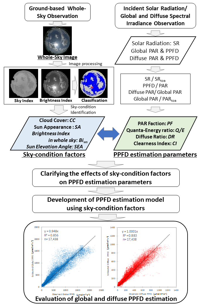
3.3. Estimation of Global and Diffuse PPFD with Instantaneous Values

The results of the MRA using the hourly data show the possibility of explaining the estimation parameters for the global and diffuse PPFD using the sky-condition factors. We estimated the global and diffuse PPFD using the sky-condition factors. The timescale of the estimation was set as an instantaneous value at the time of the acquisition of the whole-sky images with 2-min intervals. There were 91,511 instantaneous values (i.e., samples) recorded on 300 days from 24 February 2005 to 7 February 2006. To include the data observed under various sky conditions in all seasons in the samples for the model derivation and its validation, we first separated 17,438 samples obtained on 59 days (i.e., day 5, 10, 15, 20, 25, and 30 of each month) for the validation of our estimation models. Thus, we used 74,073 samples obtained on 241 days for the model derivation of the estimation parameters. We also applied an MRA to derive each estimation model of the CI_par, DR, Q/E_(g), and Q/E_(d) as response variables using the sky-condition factors as explanatory variables. In this analysis, we separated the 74,073 samples into two classes of SA = 1 and SA = 0 because the instantaneous value of the PPFD is affected most by the appearance of the sun. The number of samples in the group with SA = 1 and SA = 0 was 30,894 and 43,179, respectively.

The estimation models of the global and diffuse PPFD were constructed using four functions for SA = 1 and SA = 0 each. Here, the PF was not needed because it is possible to estimate the global PAR directly by estimating the CI_par. The models for the case of the sun appearing (i.e., SA = 1) are as follows:

$$C{I}_{par}= -0.2447 CC+0.4032 B{I}_{ws}+0.6386,$$

(14)

$$DR= 0.5086 CC+0.2468 B{I}_{ws}-0.0016 SEA+0.1764,$$

(15)

$$Q/E_{\left(g\right)}= 0.0727 CC-0.0155 B{I}_{ws}-0.0005 SEA-0.1285 DR+4.626,$$

(16)

$$Q/E_{\left(d\right)}= 0.2030 CC+0.0794 B{I}_{ws}+0.0004 SEA+4.311.$$

(17)

The models for the case of the sun hidden by cloud (i.e., SA = 0) are written as follows:

$$C{I}_{par}= -0.1271 CC+0.9823 B{I}_{ws}-0.0049 SEA+0.3239,$$

(18)

$$DR= 0.3078 CC-0.2696 B{I}_{ws}+0.0007 SEA+0.6912,$$

(19)

$$Q/E_{\left(g\right)}= 0.1748 CC+0.0263 B{I}_{ws}-0.0004 SEA-0.2755 DR+4.651,$$

(20)

$$Q/E_{\left(d\right)}= 0.2010 CC+0.0448 B{I}_{ws}-0.0002 SEA+4.344.$$

(21)

These model equations were created using only explanatory variables that are considered statistically significant (i.e., having a p-value of <0.001). However, we could not derive the multiregression model for the Q/E_(g) using only sky-condition factors. Therefore, similarly to the estimation models of the Q/E_(g) shown in Equations (16) and (20), the DR was used as one of the explanatory variables. In the case of estimating the Q/E_(g), we used the DR estimated using Equations (15) and (19), together with the CC, BI_ws, and SEA.

To evaluate the contribution of each explanatory variable in the MRA,

Table 3. Standard partial regression coefficients and multiple coefficient of determination (R²) in the case of SA = 1 (n = 30,894).

Standard Partial Regression Coefficient	CC	BIws	SEA	DR	R2
CIpar	−0.438	0.261			0.156
DR	0.680	0.119	−0.127		0.520
Q/E(g)	0.713	−0.055	−0.278	−0.943	0.509
Q/E(d)	0.783	0.104	0.083		0.741

All explanatory variables have p-values of <0.001.

and

Table 4. Standard partial regression coefficient and multiple coefficient of determination (R²) in the case of SA = 0 (n = 43,179).

Standard Partial Regression Coefficient	CC	BIws	SEA	DR	R2
CIpar	−0.136	0.939	−0.653		0.599
DR	0.452	−0.353	0.127		0.273
Q/E(g)	0.678	0.091	−0.218	−0.727	0.564
Q/E(d)	0.665	0.132	−0.067		0.455

All explanatory variables have p-values of <0.001.

list the standard partial regression coefficients of the CC, BI_ws, SEA, and DR (used only for the Q/E_(g)) with the multiple coefficient of determination (R²) of each model, for SA = 1 and SA = 0 respectively.

The values of R² of the CI_par in the case of SA = 1 and of the DR in the case of SA = 0 are low, i.e., 0.156 and 0.273, respectively. This is because the values of the CI_par when the sun appears (SA = 1) and of the DR when the sun is hidden (SA = 0) do not change greatly when distinguishing samples for SA = 1 and SA = 0. Overall, the CC has a positive effect on the DR, Q/E_(g), and Q/E_(d) in the two cases where SA = 1 and SA = 0. In the case of SA = 0, the BI_ws contributes positively to the CI_par, while the SEA affects the CI_par negatively. On the hourly timescale, the BI_ws and SEA are not adopted as explanatory variables for the DR and Q/E_(d), respectively (Table 2), but in the data samples with the instantaneous values, the BI_ws contributes to the DR positively (SA = 1) and negatively (SA = 0), while the SEA contributes slightly to the Q/E_(d). By separating the two cases of the sun appearing and being hidden, the sky-condition factors seem to function interactively in explaining each estimation parameter.

We then applied the estimation models expressed as Equations (14)–(21) to the sky-condition factors of the validation samples (n = 17,438), and calculated the estimated global PPFD (PPFD_{g_e}) and diffuse PPFD (PPFD_{d_e}) using Equations (10) and (11). To evaluate our estimation, the relationship between the observed global and diffuse PPFD and the estimations derived using the instantaneous values is shown in the left and right panels of Figure 3, respectively. A linear approximation with a zero intercept is shown in each panel of the figure. The coefficient for the global and diffuse PPFD is 0.948 and 1.0001, respectively, i.e., both coefficients are close to 1.0. The coefficient of determination (R²) for both relationships is >0.85.

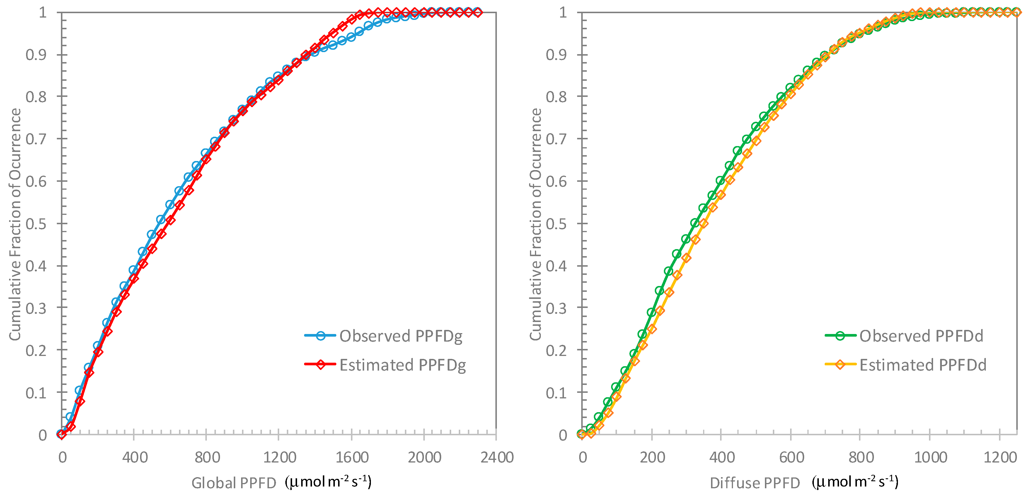
Figure 4 shows the cumulative frequency distribution curves [35] of the estimated and the observed PPFD. For the global PPFD (Figure 4; left), a difference of about 3% between the estimated value and the observed value was found at around 500–700 μmol m⁻² s⁻¹. Moreover, the curves of both agree well until 800–1400 μmol m⁻² s⁻¹. A difference of 3–4% can again be seen at around 1450–1750 μmol m⁻² s⁻¹. The global PPFD with instantaneous values over 1750 might be difficult to estimate in this model. As for the diffuse PPFD (Figure 4; right), a difference of 3–5% can be seen at around 200–500 μmol m⁻² s⁻¹; however, the two curves are otherwise in good agreement.

To compare our results with the results of existing methods, the estimation accuracy of the global and diffuse PAR and PPFD is summarized in

Table 5. Mean, mean error, RMSE, and relative RMSE of the global and diffuse PAR and PPFD estimations made with instantaneous values.

Statistics	PARg (W m−2)	PARd (W m−2)	PPFDg (μmol m−2 s−1)	PPFDd (μmol m−2 s−1)
Mean	142.24	84.64	649.74	381.33
Mean error	0.51	3.16	1.77	14.00
RMSE	37.73	16.40	174.55	75.07
RMSE (%)	26.6	20.1	26.9	20.4

. The mean bias errors of the global and diffuse PAR (PPFD) were 0.51 W m⁻² (1.77 μmol m⁻² s⁻¹) and 3.16 W m⁻² (14.0 μmol m⁻² s⁻¹), respectively. The diffuse components of the PAR and PPFD tend to be somewhat overestimated in comparison with the global PAR and PPFD. However, the relative root mean square error (RMSE) of the diffuse component is less than the global RMSE. The most remarkable point is that the relative RMSEs of the global PAR and PPFD and diffuse PAR and PPFD are almost the same, indicating that our models of the Q/E_(g) and Q/E_(d) contribute much to the estimation of the PPFD.

Wang et al. [36] estimated the global PPFD using hourly data of the CI and a cosine SEA function with a relative RMSE of 7.0–12.5% at meteorological stations in China. In the case of estimating the global PPFD using instantaneous values of the CI, Sun et al. [37] obtained an RMSE of 40%. In the case of the diffuse PPFD estimation, Jacovides et al. [38] performed estimations using the CI_par and DR with a relative RMSE of 27% on an hourly timescale. Wang et al. [39] estimated the hourly global and diffuse PPFD under clear sky conditions at sites having a complex terrain using the ratios of the global and diffuse PAR to extraterrestrial PAR, and they reported relative RMSEs of 8–26% and 23–26%, respectively. Our estimations of the global and diffuse PPFD using instantaneous values under various sky conditions with relative RMSEs of 27% and 20%, respectively, have good accuracy in comparison with the results of existing methods.

3.4. Validity of PPFD Estimation with Instantaneous Values

The incident global and diffuse PPFDs on a short timescale are important input parameters for the precise modeling of plant physiological processes in the estimation of the carbon gain, biomass, and yields during vegetation growth [1,7,39,40]. To verify the validity of the estimations of the global and diffuse PPFD with instantaneous values, we examined our estimation results at daily and diurnal levels.

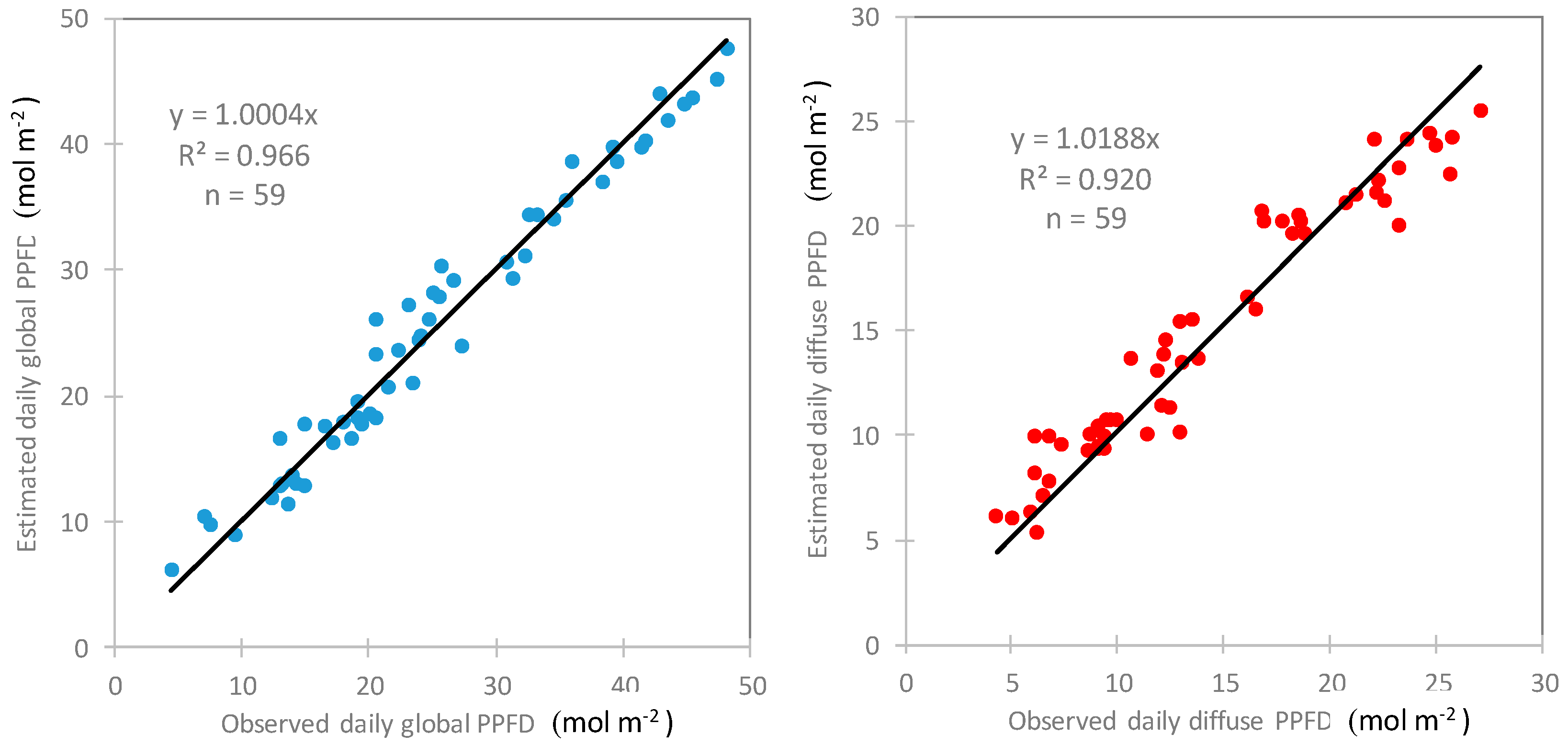
First, the relationships between the estimated and observed daily accumulated values of the global and diffuse PPFD are shown in Figure 5. The validation data for all 59 days produce a mean relative error and relative RMSE of the daily accumulated global (diffuse) PPFD of +0.9% (+4.4%) and 8.2% (11.5%), respectively (

Table 6. Mean, mean error, RMSE, and relative RMSE of the daily global and diffuse PPFD estimations.

Statistics	Daily Global PPFD	Daily Diffuse PPFD
Mean (mol m−2)	24.36	14.29
Mean error	0.22	0.61
RMSE	1.98	1.57
RME (%)	8.2	11.5

). Those days that show a low accumulation of the PPFD tend to have a large relative error of approximately 20–30%. There were 2 days on which the daily global PPFD had a relative error of >30%. The daily global PPFD on these days was low, i.e., 7.1 and 4.5 mol m⁻² d⁻¹. The whole-sky images acquired on these days showed a persistent dark cloud.

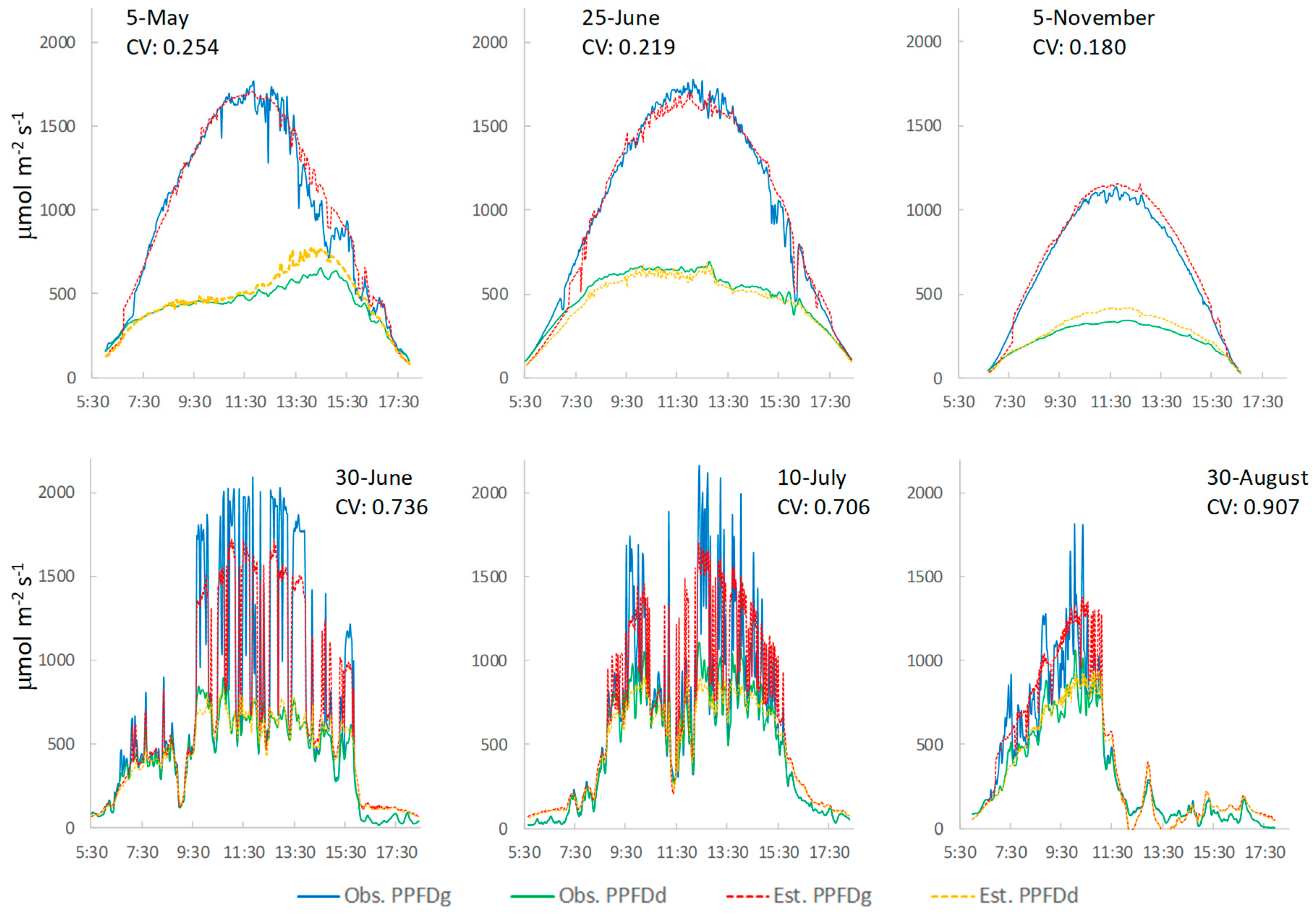
Second, we examined whether the diurnal fluctuation of the PPFD due to a change of sky condition could be estimated using instantaneous values. Using the coefficient of variation (CV = St.Dev./Mean) of the CI_par per day for all 59 days, it was assumed that a day with a large CV was a day on which sky conditions fluctuated, whereas a day with a small CV was a day on which sky conditions were clear. We selected 3 days with the lowest (0.180, 0.219, and 0.254) and 3 days with the highest (0.907, 0.736, and 0.706) CV values as days with clear and fluctuating sky conditions, respectively. The CV mean (St.Dev.) of all 59 days was 0.433 (0.147). Figure 6 shows the diurnal changes in the observed global and diffuse PPFD and the estimations made with instantaneous values for the 3 days with clear sky conditions (5 May, 25 June 5, and 5 November) and for the 3 days with fluctuating sky conditions (30 June, 10 July, and 30 August). The daily accumulated values of the observed and estimated PPFD are given in

Table 7. Daily accumulated values of the observed and estimated global and diffuse PPFD on 3 days with clear sky conditions (5 May, 25 June, and 5 November) and 3 days with fluctuating sky conditions (30 June, 10 July, and 30 August).

Date	5-May	25-June	30-June	10-July	30-August	5-November
CV of CIpar	0.254	0.219	0.736	0.706	0.907	0.180
Obs. PPFDg	42.83	48.20	30.90	26.63	16.58	24.83
Est. PPFDg	44.12	47.63	30.77	29.25	17.74	26.10
Error %	+2.9	−1.2	−0.4	+9.0	+6.5	+4.9
Obs. PPFDd	18.67	22.62	18.86	21.20	13.04	8.68
Est. PPFDd	20.20	21.18	19.64	21.47	13.49	10.03
Error %	+7.6	−6.8	+4.0	+1.3	+3.3	+13.5

.

On the 3 days when the weather was clear, both the global and the diffuse PPFD increased in the morning and decreased in the afternoon in response to the sun elevation, because there were no cloud effects. On the afternoon of 5 May, as the CC increased and the BI_ws was high, it seems that the diffuse component was greater owing to the presence of thin clouds. There were occasional differences between the observed and estimated values of the diffuse PPFD in the afternoon of 5 May and around noon on 5 November, with relative errors of the daily accumulated PPFD of +7.6% and +13.5%, respectively. In contrast, for the 3 days with fluctuating sky conditions, it can be seen that the diurnal global and diffuse PPFD changed drastically in a short time owing to the changing sky conditions, especially when the sun emerged from or disappeared behind a moving cloud. These fluctuations almost have the same pattern for the observed and estimated values, i.e., the estimated PPFD values reflect the drastic changes in sky condition at the times when the whole-sky images were acquired. However, when the observed PPFDg becomes instantaneously high, a large difference from the estimated PPFDg is evident. The absolute error in the instantaneous value is large when the sun emerges from or disappears behind a cloud. In terms of the daily accumulated values (Table 7), the relative errors of the global and diffuse PPFD are small (ranging from −0.4 to +9.0%), even on the 3 days with fluctuating sky conditions.

From Table 7 it can be seen that there were no marked differences in the relative error of the daily accumulated value between the clear days and days with fluctuating sky conditions. The process models of ecosystems are generally inputs with a time series of parameters, and they predict accumulated values. In the case of the process of photosynthesis, daily accumulating values are affected by diurnal changes in the PPFD [1,40]. 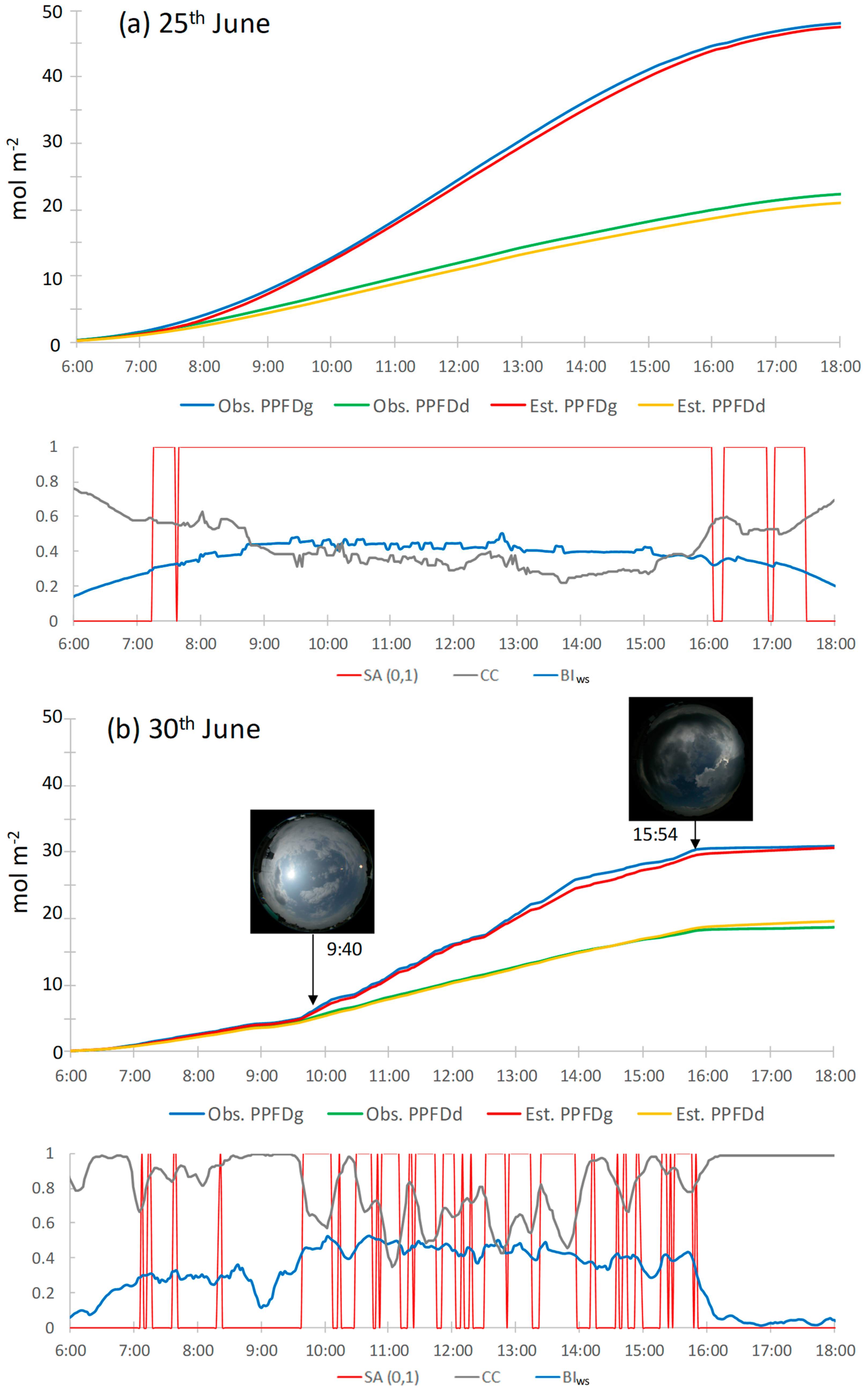Therefore, it is not possible to reflect the diurnal variation of sky conditions using only a daily value of the PPFD [1]. Here, to compare the diurnal accumulating values between the observed and estimated PPFD, Figure 7 shows the accumulating values for a time series of global and diffuse PPFD on 25 and 30 June (as an example of a clear day and a day with fluctuating sky conditions, respectively) when the SEA was high. The diurnal changes of the SA, CC, and BI_ws are also shown.

On 25 June, when the sky conditions were reasonably clear (CV = 0.219), both the global and the diffuse PPFD produced smooth curves (Figure 7a). The difference between the global and diffuse PPFD is the direct component. On this day, there was direct sunlight from early morning, and the relative errors of the daily estimated global and diffuse PPFD were −1.2% and −6.8%, respectively (Table 7). The sky conditions on 30 June were variable (CV = 0.736), i.e., after being cloudy in the early morning, it was sunny until early evening when it became cloudy again. The values of the global and diffuse PPFD were almost the same until around 09:40 local time (LT). The global PPFD increased with the appearance of the sun (i.e., the direct component increased) from 09:40 LT until around 16:00 LT. The traces of the global and diffuse PPFD were almost parallel after 16:00 LT (Figure 7b). The diurnal accumulated values of the estimated global and diffuse PPFD were always close to the observations at all times. The relative errors of the global and diffuse PPFD were −0.4% and +4.2%, respectively (Table 7). This result reflects the effects of the sky conditions well.

The above verification shows that our PPFD estimation using instantaneous values could be effective for precise process models of vegetation photosynthesis. Additionally, we expect our proposed methodology for PPFD estimation using whole-sky images to be used not only at existing weather stations but also at any point where a whole-sky camera system could be installed.

4. Conclusions

To develop a methodology for estimating the global and diffuse PPFD using ground-based whole-sky images, we examined the effects of sky-condition factors derived from whole-sky images on the estimation parameters of the PF, Q/E, DR, and CI on an hourly timescale, and then estimated the global and diffuse PPFD using instantaneous values under various sky conditions.

Regarding the effects of the sky condition on the PPFD estimation parameters, four sky-condition factors (i.e., CC, SA, BI_ws, and SEA) affected each parameter (i.e., the PF, the Q/E in the global and diffuse PAR, the DR, and the CI). It was found that the Q/E_(g) was affected mainly by the SA with a positive effect, the Q/E_(d) was strongly and positively affected by the CC, the DR was affected positively by the CC and negatively by the SA, and the CI was affected by all four factors of sky condition interactively.

Our estimation results of the global and diffuse PPFD showed good agreement with the observed PPFD, and they had a high or equivalent accuracy compared with the results of existing methods based on the data acquired at meteorological stations. Specifically, our models of the Q/E_(g) and Q/E_(d) contributed much to the estimation of the global and diffuse PPFD from the PAR. In addition, the estimated values of the global and diffuse PPFD reflected the drastic changes in sky conditions. The findings of the present study could contribute to the application of process models at the community level in relation to local ecosystems.

For the spatial estimation of the global and diffuse PPFD, it will be necessary to observe the sky condition spatially. As future work, we plan to expand our methodology to clarify the spatial PPFD distribution according to multipoint observations of the sky condition, and to produce precise spatiotemporal estimations of the PPFD. There are extensional applications to our study assuming that ground-based sky observations could be applied across a wide area. For the validation of satellite-based observations of both clouds and the Earth’s surface, it seems that establishing a suitable observation system at any site would be useful in terms of collaborating with existing ground-based observation networks. A ground-based whole-sky observation and its application could contribute to improving the quality of satellite-derived products by covering a wide area.

References

1. Cho, J.; Oki, T.; Yeh, P.J.F.; Kanae, S.; Kim, W. The effect of estimated PAR uncertainties on the physiological processes of biosphere models. Ecol. Model. 2010, 221, 1575–1578. [Google Scholar] [CrossRef]
2. Akitsu, T.; Kume, A.; Hirose, Y.; Ijima, O.; Nasahara, K.N. On the stability of radiometric ratios of photosynthetically active radiation to global solar radiation in Tsukuba, Japan. Agric. For. Meteorol. 2015, 209, 59–68. [Google Scholar] [CrossRef]
3. Ohmura, A.; Dutton, E.G.; Forgan, B.; Fröhlich, C.; Gilgen, H.; Hegner, H.; Heimo, A.; König-Langlo, G.; McArthur, B.; Müller, G.; et al. Baseline Surface Radiation Network (BSRN/WCRP): New Precision Radiometry for Climate Research. Bull. Am. Meteorol. Soc. 1998, 79, 2115–2136. [Google Scholar] [CrossRef] [Green Version]
4. Montreith, J.L. Climate and the efficiency of crop production in Britain. Philos. Trans. R. Soc. Lond. B Biol. Sci. 1977, 281, 277–294. [Google Scholar] [CrossRef]
5. McCree, K.J. Test of current definitions of photosynthetically active radiation against leaf photosynthesis data. Agric. For. Meteorol. 1972, 10, 443–453. [Google Scholar] [CrossRef]
6. Zhang, X.; Zhang, Y.; Zhoub, Y. Measuring and modelling photosynthetically active radiation in Tibet Plateau during April-October. Agric. For. Meteorol. 2000, 102, 207–212. [Google Scholar] [CrossRef]
7. Dye, D.G. Spectral composition and quanta-to-energy ratio of diffuse photosynthetically active radiation under diverse cloud conditions. J. Geophys. Res. D Atmos. 2004, 109, 1–12. [Google Scholar] [CrossRef]
8. Finch, D.A.; Bailey, W.G.; McArthur, L.J.B.; Nasitwitwi, M. Photosynthetically active radiation regimes in a southern African savanna environment. Agric. For. Meteorol. 2004, 122, 229–238. [Google Scholar] [CrossRef]
9. Jacovides, C.P.; Timvios, F.S.; Papaioannou, G.; Asimakopoulos, D.N.; Theofilou, C.M. Ratio of PAR to broadband solar radiation measured in Cyprus. Agric. For. Meteorol. 2004, 121, 135–140. [Google Scholar] [CrossRef]
10. Jacovides, C.P.; Tymvios, F.S.; Assimakopoulos, V.D.; Kaltsounides, N.A. The dependence of global and diffuse PAR radiation components on sky conditions at Athens, Greece. Agric. For. Meteorol. 2007, 143, 277–287. [Google Scholar] [CrossRef]
11. Ge, S.; Smith, R.G.; Jacovides, C.P.; Kramer, M.G.; Carruthers, R.I. Dynamics of photosynthetic photon flux density (PPFD) and estimates in coastal northern California. Theor. Appl. Climatol. 2011, 105, 107–118. [Google Scholar] [CrossRef]
12. Aguiar, L.J.G.; Fischer, G.R.; Ladle, R.J.; Malhado, A.C.M.; Justino, F.B.; Aguiar, R.G.; da Costa, J.M.N. Modeling the photosynthetically active radiation in South West Amazonia under all sky conditions. Theor. Appl. Climatol. 2012, 108, 631–640. [Google Scholar] [CrossRef]
13. Wang, L.; Gong, W.; Ma, Y.; Hu, B.; Zhang, M. Photosynthetically active radiation and its relationship with global solar radiation in Central China. Int. J. Biometeorol. 2013, 1265–1277. [Google Scholar] [CrossRef]
14. Wang, L.; Gong, W.; Lin, A.; Hu, B. Analysis of photosynthetically active radiation under various sky conditions in Wuhan, Central China. Int. J. Biometeorol. 2014, 58, 1711–1720. [Google Scholar] [CrossRef]
15. Yu, X.; Wu, Z.; Jiang, W.; Guo, X. Predicting daily photosynthetically active radiation from global solar radiation in the Contiguous United States. Energy Convers. Manag. 2015, 89, 71–82. [Google Scholar] [CrossRef]
16. Freedman, J.M.; Fitzjarrald, D.R.; Moore, K.E.; Sakai, R.K. Boundary Layer Clouds and Vegetation—Atmosphere Feedbacks. J. Clim. 2001, 14, 180–197. [Google Scholar] [CrossRef]
17. Gu, L.; Baldocchi, D.; Verma, S.B.; Black, T.A.; Vesala, T.; Falge, E.M.; Dowty, P.R. Advantages of diffuse radiation for terrestrial ecosystem productivity. J. Geophys. Res. Atmos. 2002, 107, 2–23. [Google Scholar] [CrossRef]
18. Letts, M.G.; Lafleur, P.M.; Roulet, N.T. On the relationship between cloudiness and net ecosystem carbon dioxide exchange in a peatland ecosystem. Ecoscience 2005, 12, 53–59. [Google Scholar] [CrossRef]
19. Min, Q. Impacts of aerosols and clouds on forest-atmosphere carbon exchange. J. Geophys. Res. D Atmos. 2005, 110, 1–12. [Google Scholar] [CrossRef]
20. Brodersen, C.R.; Vogelmann, T.C.; Williams, W.E.; Gorton, H.L. A new paradigm in leaf-level photosynthesis: Direct and diffuse lights are not equal. Plant Cell Environ. 2008, 31, 159–164. [Google Scholar] [CrossRef]
21. Mercado, L.M.; Bellouin, N.; Sitch, S.; Boucher, O.; Huntingford, C.; Wild, M.; Cox, P.M. Impact of changes in diffuse radiation on the global land carbon sink. Nature 2009, 458, 1014–1017. [Google Scholar] [CrossRef] [Green Version]
22. Cheng, S.J.; Bohrer, G.; Steiner, A.L.; Hollinger, D.Y.; Suyker, A.; Phillips, R.P.; Nadelhoffer, K.J. Variations in the influence of diffuse light on gross primary productivity in temperate ecosystems. Agric. For. Meteorol. 2015, 201, 98–110. [Google Scholar] [CrossRef] [Green Version]
23. Escobedo, J.F.; Gomes, E.N.; Oliveira, A.P.; Soares, J. Modeling hourly and daily fractions of UV, PAR and NIR to global solar radiation under various sky conditions at Botucatu, Brazil. Appl. Energy 2009, 86, 299–309. [Google Scholar] [CrossRef]
24. Kassianov, E.; Long, C.N.; Ovtchinnikov, M. Cloud Sky Cover versus Cloud Fraction: Whole-Sky Simulations and Observations. J. Appl. Meteorol. 2005, 44, 86–98. [Google Scholar] [CrossRef]
25. Tuchida, S.; Nishida, K.; Iwao, K.; Kawato, W.; Oguma, H.; Iwasaki, A. Phenological Eyes Network for Validation of Remote Sensing. J. Remote Sens. Soc. Jpn. 2005, 25, 282–288. [Google Scholar]
26. Souza-Echer, M.P.; Pereira, E.B.; Bins, L.S.; Andrade, M.A.R. A simple method for the assessment of the cloud cover state in high-latitude regions by a ground-based digital camera. J. Atmos. Ocean. Technol. 2006, 23, 437–447. [Google Scholar] [CrossRef]
27. Calbó, J.; Sabburg, J. Feature extraction from Whole-sky ground-based images for cloud-type recognition. J. Atmos. Ocean. Technol. 2008, 25, 3–14. [Google Scholar] [CrossRef]
28. Yamashita, M.; Yosimura, M. Development of sky conditions observation method using whole sky camera. J. Jpn. Soc. Photogramm. Remote Sens. 2008, 47, 50–59. [Google Scholar]
29. Heinle, A.; Macke, A.; Srivastav, A. Automatic cloud classification of whole sky images. Atmos. Meas. Tech. 2010, 557–567. [Google Scholar] [CrossRef]
30. Kazantzidis, A.; Tzoumanikas, P.; Bais, A.F.; Fotopoulos, S.; Economou, G. Cloud detection and classification with the use of whole-sky ground-based images. Atmos. Res. 2012, 113, 80–88. [Google Scholar] [CrossRef]
31. Letu, H.; Nagao, T.M.; Nakajima, T.Y.; Matsumae, Y. Method for validating cloud mask obtained from satellite measurements using ground-based sky camera. Appl. Opt. 2014, 53, 7523. [Google Scholar] [CrossRef]
32. Katagiri, S.; Hayasaka, T.; Yamada, K. An Algorithm for a Whole-Sky Camera with Low Color Depth and Relationships Between Cloud Fractions Derived from the Sky Camera and MODIS Observation. J. Remote Sens. Soc. Jpn. 2015, 35, 89–103. [Google Scholar]
33. Nagai, S.; Akitsu, T.; Saitoh, T.M.; Busey, R.C.; Fukuzawa, K.; Honda, Y.; Ichie, T.; Ide, R.; Ikawa, H.; Iwasaki, A.; et al. 8 million phenological and sky images from 29 ecosystems from the Arctic to the tropics: The Phenological Eyes Network. Ecol. Res. 2018, 8–11. [Google Scholar] [CrossRef]
34. Thuillier, G.; Hers, M.; Simon, P.C.; Labs, D.; Mandel, H.; Gillotay, D. Observation of the solar spectral irradiance from 200 nm to 870 nm during the ATLAS 1 and ATLAS 2 missions by the SOLSPEC spectrometer. Metrologia 2003, 35, 689–695. [Google Scholar] [CrossRef]
35. Bilbao, J.; de Miguel, A.H.; Kambezidis, H.D. Air Temperature Model Evaluation in the North Mediterranean Belt Area. J. Appl. Meteorol. 2002, 41, 872–884. [Google Scholar] [CrossRef]
36. Wang, L.; Kisi, O.; Zounemat-Kermani, M.; Hu, B.; Gong, W. Modeling and comparison of hourly photosynthetically active radiation in different ecosystems. Renew. Sustain. Energy Rev. 2016, 56, 436–453. [Google Scholar] [CrossRef]
37. Sun, Z.; Liang, H.; Liu, J.; Shi, G. Estimation of photosynthetically active radiation using solar radiation in the UV-visible spectral band. Sol. Energy 2017, 153, 611–622. [Google Scholar] [CrossRef]
38. Jacovides, C.P.; Boland, J.; Asimakopoulos, D.N.; Kaltsounides, N.A. Comparing diffuse radiation models with one predictor for partitioning incident PAR radiation into its diffuse component in the eastern Mediterranean basin. Renew. Energy 2010, 35, 1820–1827. [Google Scholar] [CrossRef]
39. Wang, Q.; Tenhunen, J.; Schmidt, M.; Kolcun, O.; Droesler, M.; Reichstein, M. Estimation of total, direct and diffuse PAR under clear skies in complex alpine terrain of the National Park Berchtesgaden, Germany. Ecol. Model. 2006, 196, 149–162. [Google Scholar] [CrossRef]
40. Still, C.J.; Riley, W.J.; Biraud, S.C.; Noone, D.C.; Buenning, N.H.; Randerson, J.T.; Torn, M.S.; Welker, J.; White, J.W.C.; Vachon, R.; et al. Influence of clouds and diffuse radiation on ecosystem-atmosphere CO2 and CO18O exchanges. J. Geophys. Res. Biogeosci. 2009, 114, 1–17. [Google Scholar] [CrossRef]
Figure 1. Flow diagram of the derivation of the sky-condition factors of CC, SA, and BIws from whole-sky image processing.
Remotesensing 11 00932 g001
Figure 2. Observed monthly means of (a) the sky-condition factors of CC, SA, and BIws, (b) the PF, (c) Q/E(g), and (d) Q/E(d). The bars show the standard deviations.
Remotesensing 11 00932 g002
Figure 3. Scatter plots of the estimated and observed PPFD: (left) global PPFD and (right) diffuse PPFD (n = 17,438).
Remotesensing 11 00932 g003
Figure 4. Cumulative probability distributions of the observed and estimated PPFD with instantaneous values: (left) global PPFD and (right) diffuse PPFD.
Remotesensing 11 00932 g004
Figure 5. Scatter plots of the estimated and observed daily PPFD: (left) daily global PPFD and (right) daily diffuse PPFD (n = 59).
Remotesensing 11 00932 g005
Figure 6. Diurnal changes in the observed and estimated PPFD on 3 days with clear sky conditions (upper plots: 5 May, 25 June, and 5 November) and 3 days with fluctuating sky conditions (lower plots: 30 June, 10 July, and 30 August).
Remotesensing 11 00932 g006
Figure 7. Time series of the diurnal accumulation of the observed and estimated global and diffuse PPFD: (a) 25 June and (b) 30 June. The lower graph of each panel shows the diurnal changes of the SA (0,1), CC, and BIws in sky-condition factors.
Remotesensing 11 00932 g007