1. Introduction
Rainfall is one of the most conventional observations, which is observed by almost all the surface stations. The rainfall variable can also be derived from remote sensing measurements like satellite product. Rain gauge and satellite remote sensing have been widely used to measure precipitation. Both have been assimilated into NWP models to improve heavy rainfall forecasts [
1,
2]. On one hand, a rain gauge may provide accurate measurements of surface precipitation at a point location; however, it lacks spatial representation in complex terrain and for intense precipitation with high spatial variation [
3]. On the other hand, satellite-based precipitation products are capable of detecting spatial patterns and temporal variations of precipitation at a finer resolution, which is particularly useful over poorly gauged regions like ocean [
4]. However, satellite-based remote sensing is an indirect estimate of precipitation, inherently containing regional and seasonal systematic biases and random errors [
5,
6]. Since these errors can be corrected by merging satellite products with rain gauge data [
7], great progresses have been made in developing combined rainfall products with higher accuracy over the globe [
8,
9,
10,
11]. Recently, the National Meteorological Information Center of China Meteorological Administration has developed an operational satellite-gauge merged precipitation product with the hourly and 0.1° (~10 km) resolution (CHMPA) [
12]. This product has been widely used in many operational centers for monitoring, diagnosing and verifying heavy rainfall events. However, the CHMPA rainfall data has not been used in NWP models quantitatively, and the effectiveness of this rainfall product in data assimilation for improving rainfall forecast should be investigated.
Several approaches to assimilating precipitation observations into NWP models have been developed to improve the model initial states and the sub-consequent short-range rainfall forecasts in the past few decades. The initialization schemes, such as the dynamical initialization [
13], physical initialization [
14] and cumulus convection initialization [
15,
16] had been widely used. However, the initialization methods are indirect ways of assimilating precipitation data because they usually restructure the moisture and temperature fields. The shortcoming of these methods is that they don’t guarantee dynamically consistent initial conditions [
17]. The nudging technique [
18,
19,
20,
21,
22] is also one of the simplest and most computationally economical methods for rainfall data assimilation. However, the initial conditions generated by this method are also dynamically inconsistent [
17,
23] which is same as the initialization methods. Compared to the schemes mentioned above, the 4DVar can assimilate precipitation data directly. The major advantages of 4DVar is that it uses the full model dynamics to adjust the model variables according to the observed precipitation [
24,
25]. Zupanski and Mesinger (1995) [
26] demonstrated the technical feasibility of the 4DVar and showed an improvement of precipitation forecast using a regional forecast model and an incomplete adjoint model. Later, studies [
17,
27,
28,
29,
30,
31] indicated that the precipitation data assimilation using the 4DVar leads to reductions in the spin-up time, improving the moisture distributions in model initial conditions and the subsequent short-range rainfall forecasts. Some operational weather services have assimilated precipitation data operationally using 4DVar method to improve precipitation forecasts, including Japan Meteorological Agency (JMA) [
32] and European Centre for Medium-Range Weather Forecasts (ECMWF) [
33,
34,
35]. Therefore, the 4DVar method is used in this study to assimilate the CHMPA rainfall data into WRF model.
As the first test to assimilate a new kind of rainfall data like CHMPA in this paper, some observation-related parameters such as observation error, thinning distance, accumulated time corresponding with the 4DVar assimilation window should also be investigated. Thus, two basic questions arise in this study: How does the rainfall observation error, rainfall accumulation time within assimilation window, rainfall thinning distance for assimilation of CHMPA data using the 4DVar affect the rainfall forecasts? Will the assimilation of CHMPA rainfall data improve the rainfall forecasts using the 4DVAR approach? In this study, capability of assimilating the CHMPA rainfall data is developed within the WRF 4DVar [
36,
37]. The purpose of this study is to assimilate CHMPA rainfall data in WRFDA 4DVar and to explore its impact on heavy rainfall forecast that occurred over Jianghuai area in eastern China. A series of experiments were conducted in this study. The sensitivity of forecast skill of assimilating the CHMPA rainfall data to the rainfall observation error, the rainfall observation thinning distance, the rainfall accumulation time within 6 h assimilation window is first investigated, respectively. Then, the impact of assimilation with and without CHMPA rainfall data was evaluated.
The outline of the paper is as the follows: The data used in assimilation experiments is described in
Section 2. WRFDA 4DVar and experiments design are introduced in
Section 3. The results and discussions are presented in
Section 4. The conclusion is given in
Section 5.
2. The CHMPA Data and Preprocessing
The precipitation observations to be assimilated in this study are China Hourly Merged Precipitation Analysis (CHMPA) data, which is developed by the National Meteorological Information Center of China Meteorological Administration [
12]. The CHMPA rainfall data combines rainfall observations from satellite-retrieved CMORPH with high-density, hourly automatic weather stations rainfall data, utilizing a two-step merging algorithm. The merging algorithm combines a probability density function (PDF) matching method and optimal interpolation (OI) which was developed by Xie and Xiong (2011) [
7]. The global CMORPH precipitation estimates have a temporal interval of 30 min and a horizontal resolution of 8 km covering the area between 60°S and 60°N [
38]. To generate the merged rainfall data, the CMORPH precipitation is accumulated to an hourly rate and also interpolated onto a horizontal resolution of 0.1° in latitude and longitude. The hourly rain gauge data at more than 30,000 automatic weather stations over China which have been under quality control [
39] are used. Then, the quality-controlled hourly rain gauge data are interpolated onto regular grid points with a spatial resolution of 0.1° over the mainland China using a modified climatology-based OI interpolation algorithm [
40,
41]. So far, the CHMPA rainfall data are available on China meteorological data network (
http://data.cma.cn/data). The precipitation observations data used in this study had been converted into the WRFDA readable data format. Observations with innovations greater than three times the assumed observation error standard deviation were rejected.
4. Results
4.1. Single Observation Test
Single observation experiment helps to gain intuitive understanding of the workings of data assimilation system, as they characterize the correlations between variables and the structure of the background error covariance used in the analysis update. The spatial spread of analysis increment is primarily determined by the spatial correlation in the background error covariance and how this is propagated throughout the assimilation window by the ADM. Thus, the assimilation of rainfall data using 4DVar mainly has impact on wind variables, moisture variables and rainfall variables. The structure of the background error covariance can be flow-dependent in 4DVar because of the implicit evolution by the ADM, although the background error covariance at the start of the assimilation window is still based on climatological method such as NMC. To the author’s knowledge, the single rainfall observation test has been rarely studied before. To investigate how the background error covariance in 4DVar influences the assimilation of rainfall data, a single rainfall observation is assumed to be located at the position (32°N, 116°E) at the surface at 0006 UTC 05 July 2013 and then assimilated into WRF model in this study. The value of the rainfall observation is set to 10 mm with an error of 2 mm. The background value of rainfall at this point is 5.3 mm (i.e., the rainfall innovation is 4.7 mm). In this test, the backgrounds are the 6 h forecasts after 1 days of 6 hourly 4DVar analysis cycles employing the full set of observations.
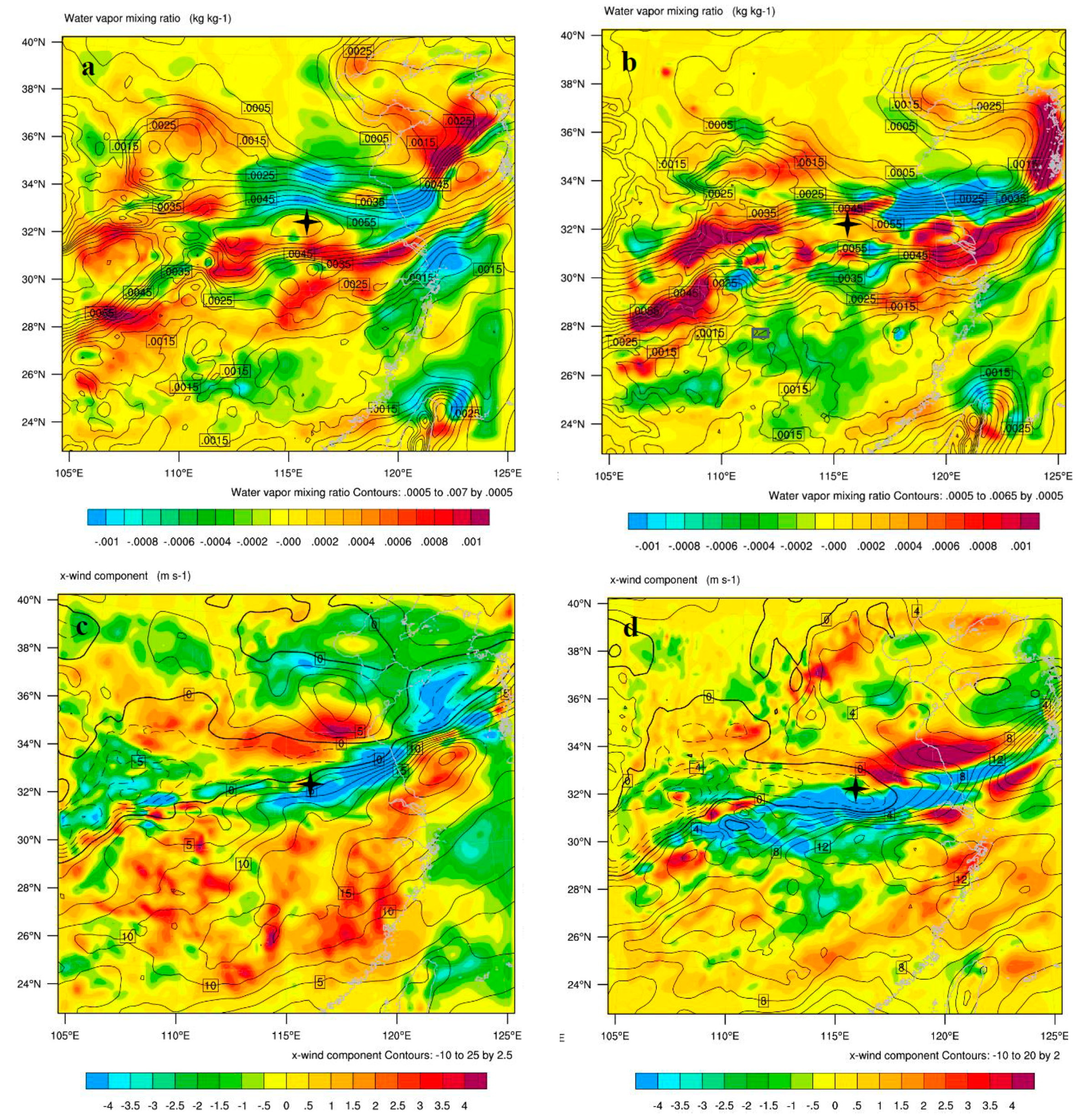
The analysis increments created by the single rainfall observation are shown by
Figure 5. The solid black lines are contours of the backgrounds at analysis time and the shaded contours are the analysis increments.
Figure 5a,b shows the analysis increments of humidity at the starting and ending time of the assimilation window.
Figure 5c,d shows the analysis increments of zonal wind at the starting and ending time of the assimilation window. It is found that the increments at the ending of the assimilation window are apparently larger than the starting of the assimilation window, and the increments distribute roughly along the background contours showing the characteristic of flow-dependence, this is because of the implicit evolution of the background error covariance contributed by the dynamic and thermodynamic balance constraints of the adjoint model. The analysis increments have a considerably larger spatial extension as they are based on climatological correlations at the start of the assimilation window [
56]. It is also found that the assimilation of rainfall has indirect impacts on wind fields through multivariate correlations and the adjoint model. In addition, the analysis increments look noisy, this may be because the single rainfall observation includes the information of multi-variables such as humidity, temperature, and wind, which all have impact on the final analysis increments through the spatial correlation of implicit-evolved background error covariance and the dynamical equations in the adjoint model.
Figure 6 shows the accumulation rainfall observation (
Figure 6a) and analysis increments of the rainfall (
Figure 6b) within the 6 h assimilation window. It is apparent that, although the model under-predicts rainfall amounts, it matches the distribution of observations located at the maximum center of the rainfall area, indicating that the assimilation of rainfall data using this WRF 4DVar system can produce direct impact on the rainfall expectations.
4.2. Real Observation Experiments
After the single rainfall observation test, the real observations experiments are conducted using the CHMPA rainfall data. The sensitivity of forecast skill of assimilating the CHMPA rainfall data to the parameters related to observation such as the rainfall observation error, the rainfall observation thinning distance and the rainfall accumulation time within 6 h assimilation window is investigated in those experiments, respectively. Then, the impact of simultaneous assimilation of CHMPA data and conventional observations is studied based on the optimal configurations selected by those sensitivity experiments. In this study, the rainfall scores are averaged over the forecasts from the 10 days cycling experiments.
To evaluate the impacts of those parameters, the rainfall forecast skill scores such as Threat Score (TS) and Fractions Skill Score (FSS) against the observations are calculated in this study. The Threat Score which is one of the most widely used point-to-point objective method, is given by
which means that TS = (hits)/(hits + false alarms + misses). Its range is 0 to 1, with a value of 1 indicating a perfect forecast. The TS is relatively frequently used, with good reason. It takes both false alarms and missed events into account, and is therefore, a more balanced score. Fractions Skill Score (FSS) is one of the neighborhood verification approaches which is calculated to evaluate the precipitation forecast skill [
57]. The FSS is defined as
where N is the number of neighborhoods;
is the proportion of grid boxes within a forecast neighborhood where the prescribed threshold is exceeded (i.e., the proportion of grid boxes that have forecast events); and
is the proportion of grid boxes within an observed neighborhood where the prescribed threshold is exceeded (i.e., the proportion of grid boxes that have observed events). In the formula the denominator represents the worst possible forecast (i.e., with no overlap between forecast and observed events). FSS ranges between 0 and 1, with 0 representing no overlap and 1 representing complete overlap between forecast and observed events, respectively. The influence distance of the neighborhood used in this study is 20 km which is the same with the data assimilation resolution.
Besides the rainfall forecast skill scores, additional variable fields are analyzed to show how the assimilation of CHMPA rainfall data influences the eventual rainfall forecasts.
4.2.1. Impacts of Rainfall Observation Error
When dealing with a new type of observation in data assimilation system, it is important to estimate the observations error [
58]. Since the CHMPA rainfall data has not been assimilated before, it is necessary to firstly investigate its appropriate error. Many previous studies have assigned the observed rainfall error empirically based on the source of the observation, the length of the precipitation accumulation period and methods of data preprocessing. For example, Zupanski and Mesinger (1995) used an observed precipitation error of only 0.001 mm for 24 h accumulated precipitation which is derived from simulated observation [
26]. Zou and Kuo (1996) using 0.045 mm for 3 h accumulated precipitation [
17]. Guo et al. (2000) used the error of 3 mm for 1 h accumulated precipitation [
28]. In WRF 4DVar, observation errors are assumed as uncorrelated in both space and time, the observational error covariance matrices are simple diagonal with rainfall observation error as elements. This observation error is considered as constant in space and time. Accurate estimation of rainfall error is complex because of its high spatial and temporal variability. Thus, a fixed observation error is used here at all the grid points. Since the information about the observation error on the CHMPA rainfall data is not available, the sensitivity of the rainfall forecast to the choice of observed rainfall error in assimilation experiments is tested in this sub-section. We assigned a series of the rainfall observation error by the value of 1, 2, 3, 4, 5 mm for 6 h accumulated precipitation.
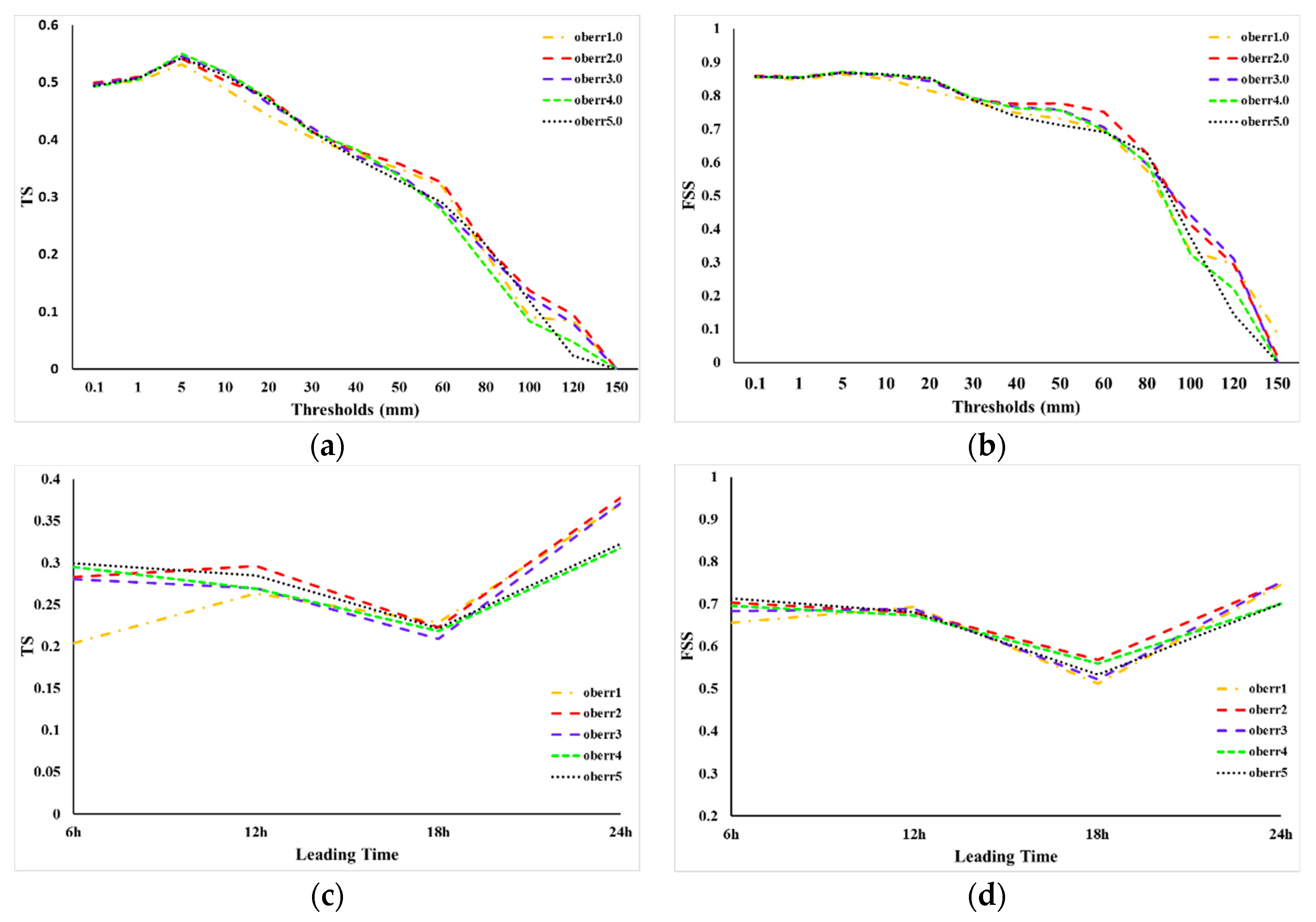
Figure 7a,b shows the TS and FSS, respectively, for 24 h accumulated precipitation forecast using the different precipitation error in data assimilation experiments. The results show that, the two verification methods generate similar results although these two methods are calculated in different ways. It is found that when the rainfall observation error is set to 2 mm, the precipitation forecast skill score performs better than the others. It is also showed that different observation error configurations have similar results when the threshold is smaller than 40 mm, except that the configuration of 1 mm observation error gets the worst result. However, the advantage of 2 mm observation error began to appear when the threshold is larger than 40 mm. When the precipitation data assimilation experiment uses 2 mm observation error, the rainfall forecast skill almost gets the highest scores, although the FSS looks lower than the 3 mm configuration at the 100 mm threshold.
Figure 7c,d show the TS and FSS, respectively, at multiple leading time. The precipitation scores are calculated at the threshold of 12 mm for every 6 h which can also represent the threshold for heavy rainfall. It is found that the TS of configuration of 1mm rainfall observation error generates the worst result for 6 h and 12 h forecasts but got comparable results with 2 mm error for 18 h forecast and 24 h forecast. It is concluded that the 1 mm error is apparently not suitable for short-range rainfall forecast. In general, the 2 mm observation error configuration performs the best. It is noted that Kumar et al, 2014 and Ban et al. 2016 also used a 2 mm rainfall observation error [
30,
31]. Therefore, 2 mm precipitation error is used in the subsequent experiments. It is noted that a fixed observation error is used at all the grid points for all rainfall thresholds in this study, although rainfall data have large spatial and temporal variability. If actual rainfall error is more (or less) than fixed observation error, the data assimilation system gives erroneously more (or less) weight to rainfall observation. Thus, the use of constant rainfall observation error in 4DVar represents a shortcoming that should be addressed in future studies [
30].
4.2.2. Impacts of Rainfall Observation Thinning Distance
Although the CHMPA rainfall data has a higher resolution in space, the assimilation of all the available rainfall data may significantly increase the computational cost brought about by the ADM and TLM in 4DVar systems. Furthermore, the error correlation between the dense rainfall observations may also cause a suboptimal data assimilation result. Thinning observations is one of the most widely used method to avoid those mentioned problems. In this study, to investigate the impact of the thinning distance on the assimilation of CHMPA rainfall data, five experiments are conducted in this subsection. The experiments include no thinning (i.e., the resolution of the full observations), 15 km thinning distance, 20 km thinning distance (i.e., the resolution of the model), 25 km thinning distance, and 30 km thinning distance. The procedure of thinning rainfall data includes (1) setting up thinning grid box (in the format of longitude and latitude) according to configuration, (2) mapping the observations to the thinning grid. Experiments results are presented in
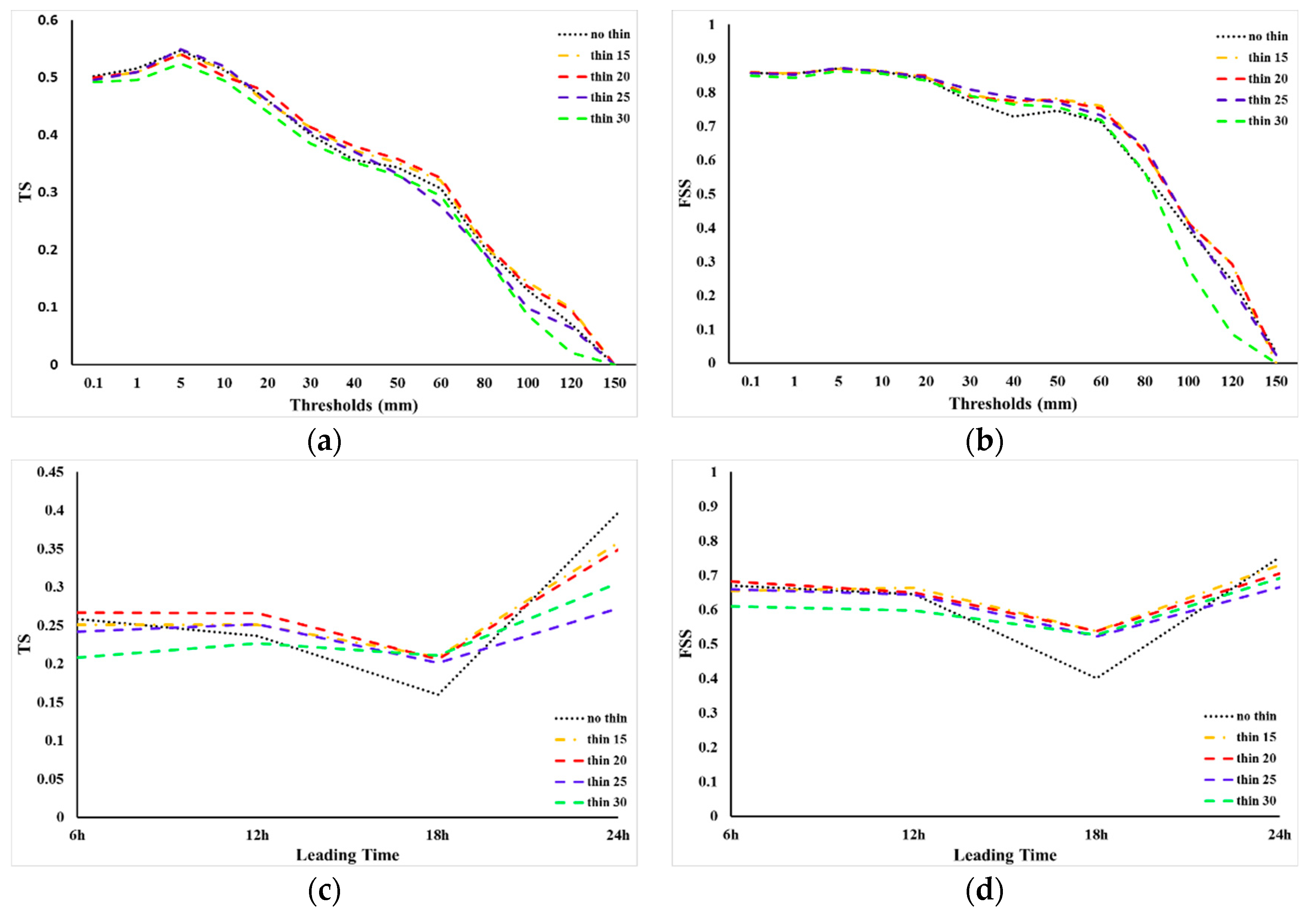
Figure 8. The threshold series of the TS and FSS for 24 h accumulated precipitation for the experiments of different thinning distance are shown in
Figure 8a,b, respectively. It can be seen that the results of experiments using 15 and 20 km thinning distance perform comparable and generated the best forecast skill at the higher scores (thresholds >50 mm for FSS and thresholds >20 mm for TS) compared with the other experiments. It is presented that the 30 km thinning distance generated the worst results, this may be due to the lack of enough rainfall observation information to match the model resolution. The experiments which assimilated the no-thinning CHMPA rainfall data also generated a unsatisfactory result, this may be caused by the error correlations between the dense rainfall observations which have a much higher resolution than the model configuration. The
Figure 8c,d shows the precipitation score with a threshold of 12.5 mm for multiple leading time, the 15 km and 20 km thinning distance still have the best results. Although their results are similar, we select the 20 km thinning distance in the following experiments because of its much lower computational cost.
4.2.3. Impacts of Rainfall Accumulation Time
WRFDA 4DVar has the capabilities to assimilate hourly, 3-hourly and 6-hourly accumulated precipitation data. To the author’s knowledge, the comparison between those different accumulation time has rarely been studied. Therefore, in order to explore the rainfall forecast performance with respect to the rainfall accumulation time within 6 h assimilation window in this study, the rainfall forecast skill against observed rainfall in the experiments with 1 h, 3 h and 6 h rainfall accumulation time are compared. The assimilation of 1 h accumulated rainfall observations needs that the rainfall observations are provided at each hour within the 6 h assimilation window, so the numbers of the rainfall observations is 6 time of the 6 h accumulated rainfall observation and two times of the 3 h accumulated rainfall data. In this study, the rainfall observation errors for the 1 h, 3 h and 6 h accumulated rainfall are fixed at 0.333 mm, 1 mm and 2 mm, respectively.
Figure 9 displays the rainfall forecast score (TS and FSS) for different configurations of rainfall accumulation time. It is found that the 6 h accumulation rainfall performs best in assimilation experiments. Its scores show apparent advantage at almost all the thresholds (
Figure 9a,b) except the threshold between 30-50 mm. It is displayed in
Figure 9c,d that the assimilation of 6 h accumulated rainfall observations generates much better rainfall forecasts especially for 6 h and 12 h leading time. The scores get close with other configurations for 18 h and 24 h leading time but still show its advantage. In this study, the 6 h accumulated rainfall assimilation within 6 h assimilation window got the best results, this may be because it is more fit to the linear assumption for 4DVar. In addition, the assimilation of 1 h and 3 h accumulated rainfall significantly increases the computational cost because of the increased observation number. Therefore, the configuration of 6 h rainfall accumulation time is used in the following experiments.
4.2.4. Impacts of simultaneous assimilation of rainfall and conventional observations
The sensitivities of forecast skill of assimilating the CHMPA rainfall data to the rainfall observation error, the rainfall observation thinning distance, the rainfall accumulated time within 6 h assimilation window have been investigated in the above experiments. The potential optimal parameters related to rainfall observation have been selected. In this subsection, we mainly study the impact of assimilating CHMPA rainfall data on the rainfall forecast skill using WRFDA 4DVar compared with assimilating conventional observations only. Three experiments are designed in this sub-section. In the first experiment, only conventional observations are assimilated (conv4dvar). In the second experiment, only CHMPA rainfall data is assimilated (pcp4dvar), and in the third experiment the CHMPA rainfall and conventional observations are simultaneously assimilated (convpcp4dvar).
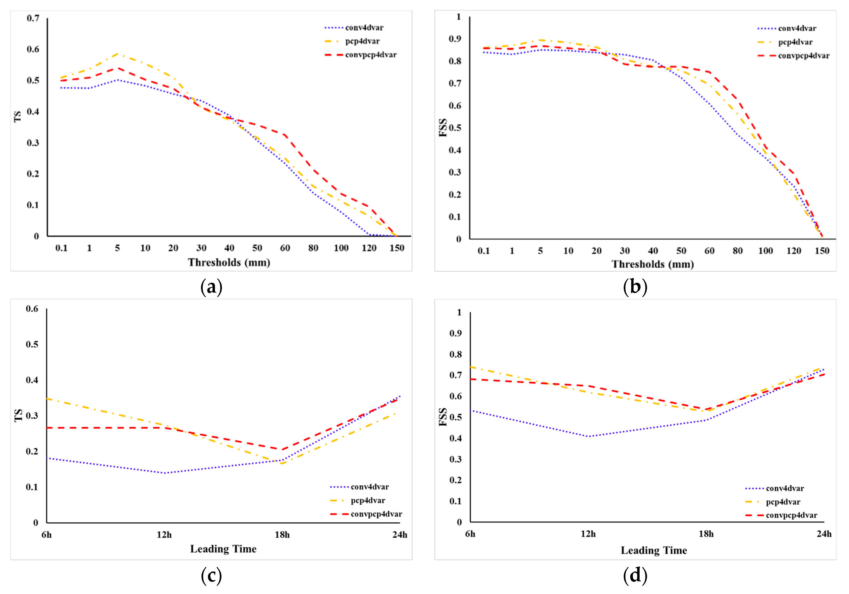
Figure 10a,b shows the threshold series of the TS and FSS for 24 h accumulated precipitation for the experiments conv4dvar, pcp4dvar and convpcp4dvar, respectively. It is apparent that the scores of these three experiments decreased with thresholds. It is also found that CHMPA rainfall observations are successfully assimilated in 4DVar because the rainfall forecast skill for experiments pcp4dvar and convpcp4dvar which assimilated the CHMPA rainfall data are systematically increased compared to the conv4dvar which did not assimilate the CHMPA rainfall data, except at the thresholds between 30 mm and 40 mm. For lower thresholds (<30 mm), the FSS and TS in pcp4dvar is larger than the conpcp4dvar. However, for higher thresholds (>50 mm), the FSS and TS in conpcp4dvar is much better than the other two experiments. The precipitation scores as a function of leading time are shown in
Figure 10c,d. The pcp4dvar and convpcp4dvar show apparent advantage over the conv4dvar at 6 h and 12 h leading time. It demonstrates that the assimilation of CHMPA rainfall data can clearly improve the spin-up problem in short-range rainfall forecasts. For 18 h and 24 h forecasts, however, the advantage of assimilating CHMPA rainfall data begin to decrease. The TS of the experiment pcp4dvar is even small than the conv4dvar, this may be caused by the imbalance introduced by assimilating the rainfall data only. In general, the convpcp4dvar performs better than the pcp4dvar except at the early leading time. This indicates that the assimilation of CHMPA rainfall data does benefit the short-range rainfall forecast, and the assimilation of conventional observations can provide constraints for the assimilation of rainfall data.
It is noted that the rainfall scores were averaged over the forecasts from the 10 days cycling experiments in this study because of the limitation of computing cost. To give robustness to the results, more experiments including various rainfall cases caused by different weather systems like Typhoon should be conducted in future work.
4.2.5. Case study
To better understand how the assimilation of CHMPA rainfall data using WRF 4DVar impacts the precipitation simulation, besides accumulated precipitation fields, additional variables such as precipitable water, vapor flux divergence, and vertical wind initialized at 0600 UTC 05 July 2013 are also diagnosed and analyzed in this sub-section.
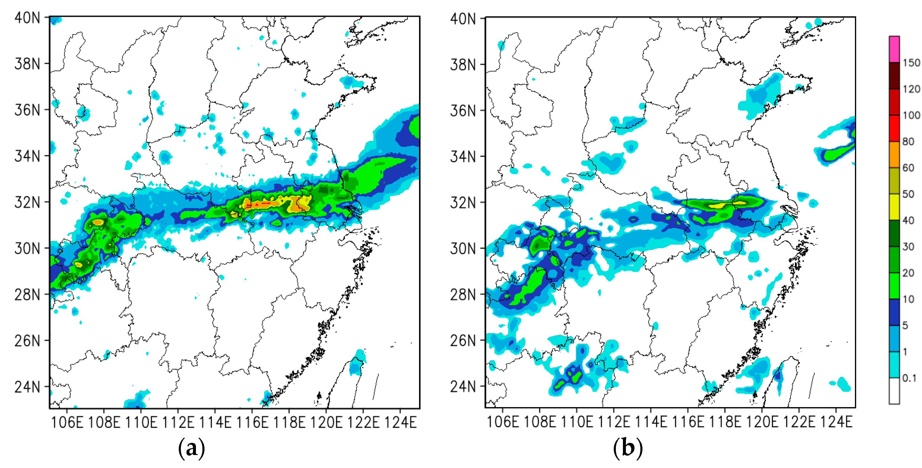
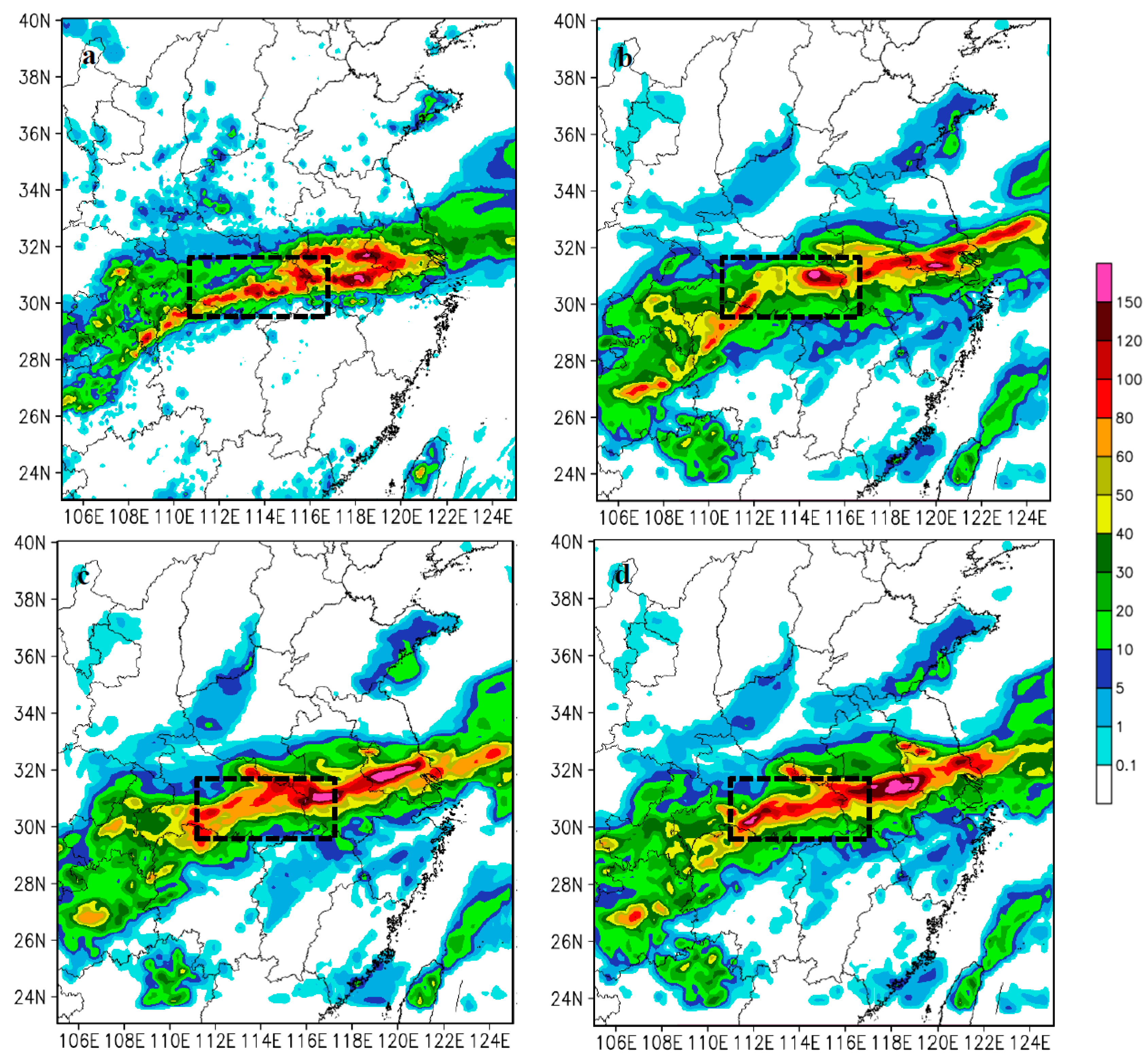
Figure 11a shows the 24 h accumulated precipitation from CHMPA rainfall data (observed precipitation). It is presented that the observed heavy rainfall is distributed roughly from southwest to the northeast across the pattern.
Figure 11b–d shows the simulated 24 h accumulated precipitation of conv4dvar, pcp4dvar, and convpcp4dvar initialized at 0600 UTC, respectively. It is found that the conv4dvar fails to simulate the precipitation amount in the black box area compared with the observation, missing the intensity and coverage of observed precipitation areas. The pcp4dvar has a little improvement in coverage but still underestimates the precipitation amount over the observed area. In comparison, the convpcp4dvar which simultaneous assimilated the rainfall and conventional observations shows much better intensity and coverage in the black box area. However, it is also found that the forecast for heavy rainfall of each configuration is not satisfactory. This indicates that the assimilation of CHMPA rainfall data needs further improved, especially for flow-dependent background error covariance and more accurate rainfall observation error.
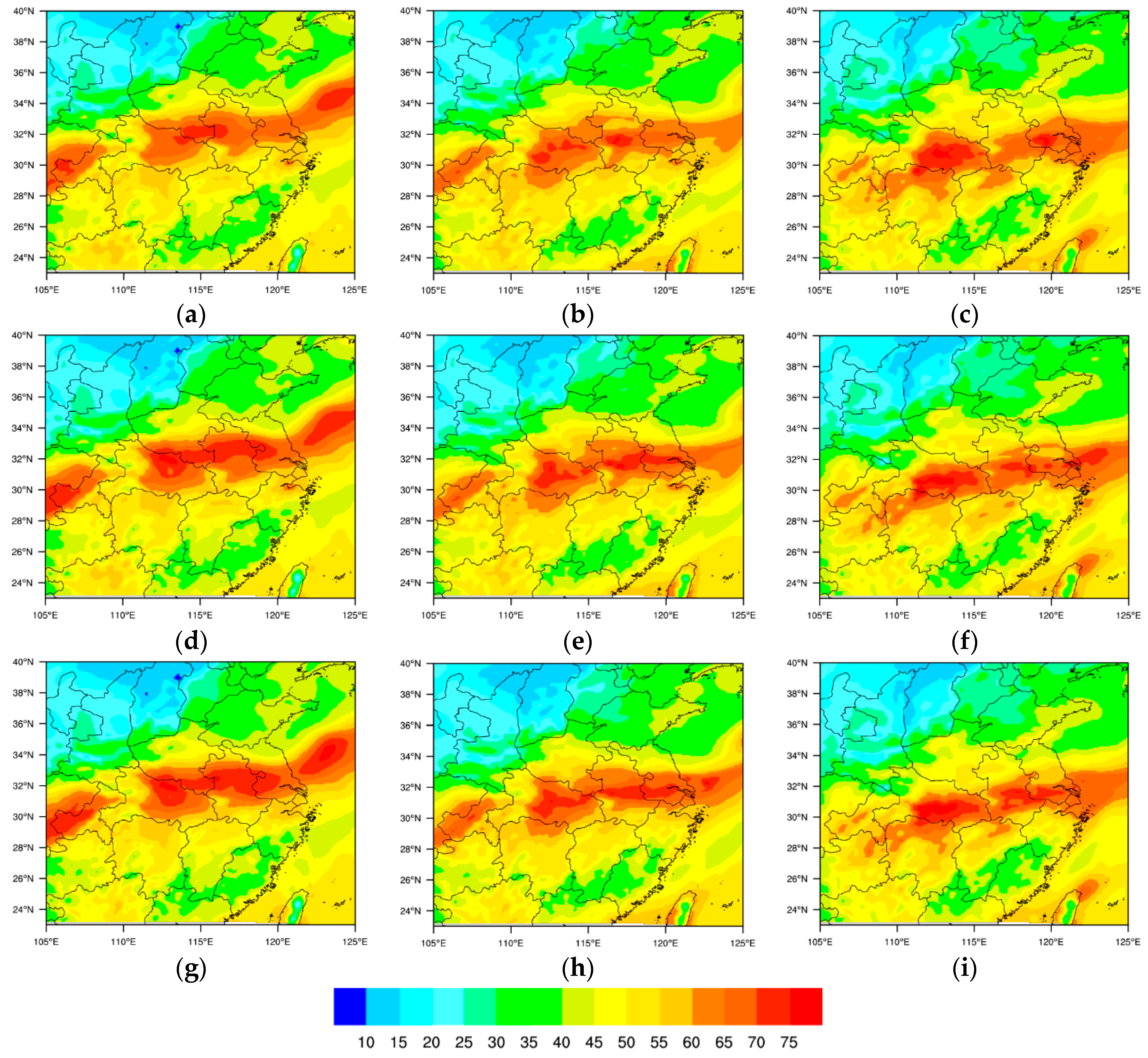
Precipitable water plays a critical role in the maintenance of a lasting heavy rainfall. The precipitable water of the analysis at 0600 UTC 05 July 2013 and its subsequent 6 h and 12 h forecasts are presented in
Figure 12. It is found that the coverage and intensity of the maximum precipitable water in conv4dvar is weaker than pcp4dvar and convpcp4dvar. This indicates that the assimilation of CHMPA tends to ameliorate the spin-up problem, especially for the analysis and 6 h forecast which is important for the extreme weather events. This also explains why the rainfall of the experiment convpcp4dvar has the best results which has been presented in the black box area in
Figure 11. For the 12 h forecast, the convpcp4dvar produces more precipitable water than the other experiments over Jianghuai area, explaining why the experiment convpcp4dvar significantly overestimates the rainfall over this area.
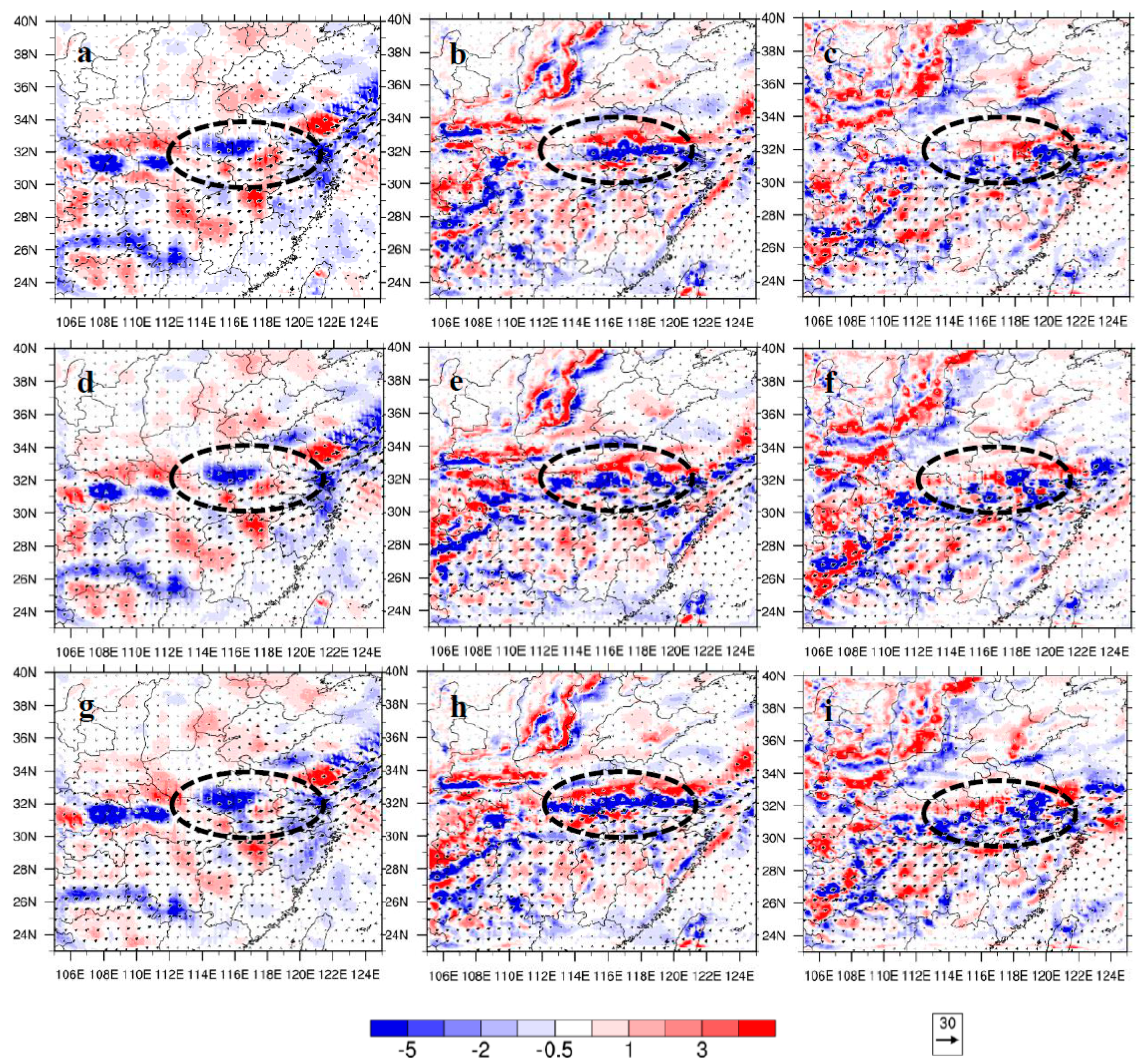
Besides, the water vapor flux divergence at 850 hPa of analyses, 6 h forecasts, and 12 h forecasts for each configuration (conv4dvar, pcp4dvar, and convpcp4dvar) initialized at 0600 UTC 05 July 2013 is presented in
Figure 13. Water vapor flux represents the direction and magnitude of the water vapor transport. It is important to investigate water vapor transport since it also plays a critical role for a persistent heavy rainfall. It is shown that the vapor flux divergence for convpcp4dvar is more widespread or stronger than that for conv4dvar and pcp4dvar over the Jianghuai area (the black box areas) where the heavy rainfall occurred, especially for 6 h and 12 h forecasts. The divergence over Hubei province of convpcp4dvar is the strongest, which is similar with the precipitable water in
Figure 12, so that it can supply sufficient moisture conditions for this area. This also explains why the simulated rainfall of the experiment convpcp4dvar over this area is the largest and also the best.
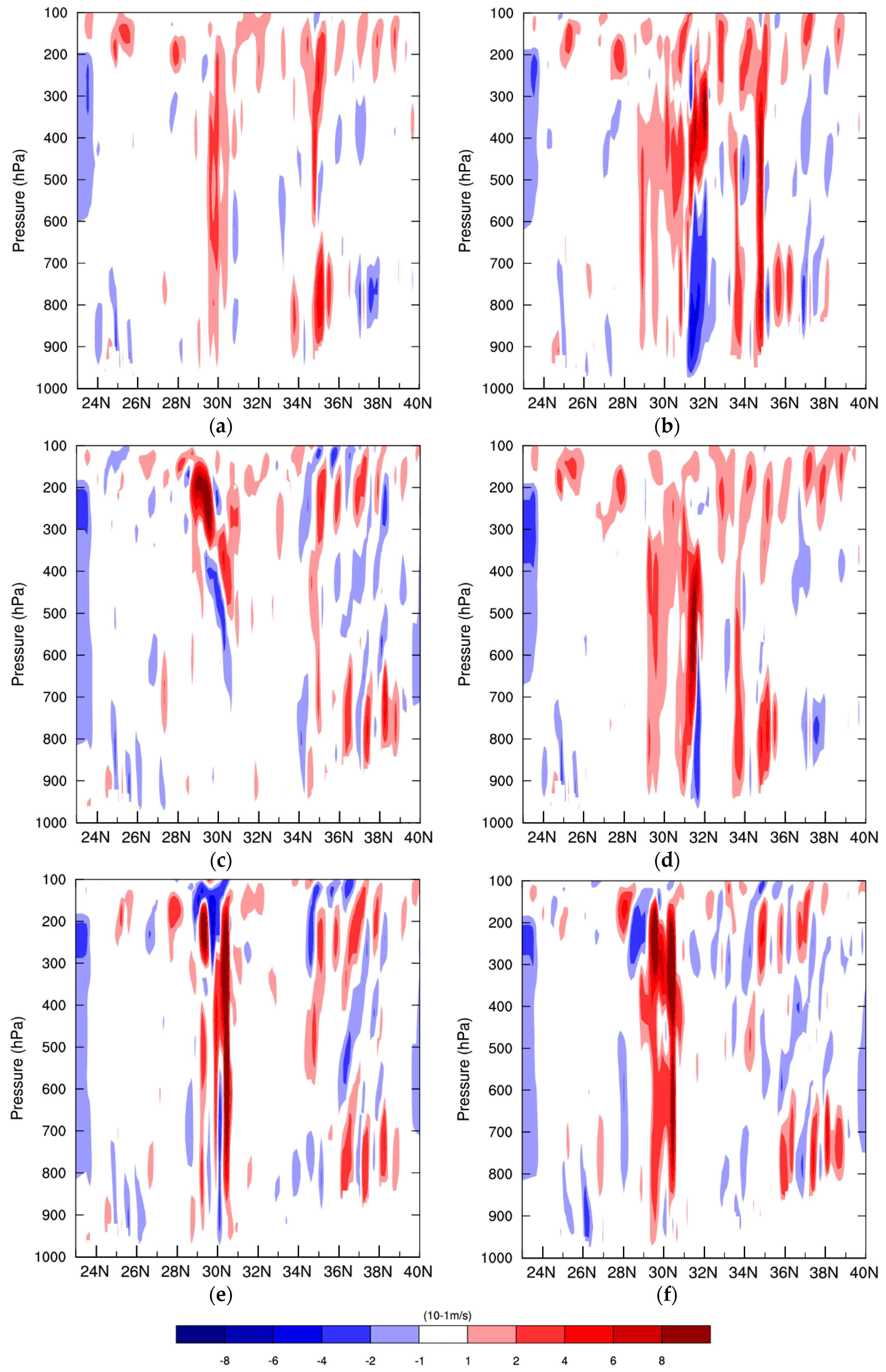
In addition, the cross sections of vertical wind along 113°E of the 6 h and 12 h forecasts initialized at 0600 UTC 05 July 2013 are shown in
Figure 14. The 113°E crosses the rainfall area around the 30.5°N. It is found that the vertical velocity of 6 h forecasts of conv4dvar and pcp4dvar are much weaker than convpcp4dvar especially in the middle and lower levels, which may eventually lead to weaker model-simulated precipitation near this area. The convpcp4dvar significantly strengthen the uplift vertical velocity, contributing to the improvement of precipitation simulation. For the 12 h forecast, the conv4dvar generates apparent downdraft in the lower level. This may have negative impact on the formation of rainfall. The convpcp4dvar has a stronger updraft than the pcp4dvar and conv4dvar throughout almost all levels. This is probably caused by the effect of dynamic constraint from the conventional observations.
5. Conclusions and Discussion
In this study, the impact of assimilating China Merged Precipitation Analysis (CHMPA) data on the rainfall forecast over Jianghuai area in eastern China is investigated. The CHMPA rainfall data is derived at China Meteorological Administration (CMA) by merging the CMORPH satellite precipitation product with rain gauge data. The WRF-4DVAR is employed in this study. A series of experiments including single rainfall observation test and real observation experiments were conducted to show how the assimilation of CHMPA data impact the rainfall forecasts.
The single observation test which assimilated a single rainfall observation shows that the increments of wind, humidity and rainfall show the characteristics of flow-dependence and multi-variable correlations because of the effect of adjoint model and background error covariance. The results of assimilating real observations show that the precipitation forecast skill of assimilating the CHMPA rainfall data using 4DVar is sensitive to the rainfall observation error, the rainfall observation thinning distance, and the rainfall accumulation time within 6 h assimilation window. The 2 mm observation error configuration in assimilation of CHMPA rainfall data using WRFDA 4DVar performs better than the other configurations in this study. The 15 km and 20 km thinning distance in this study have similar results, but the latter one needs much lower computational cost. In this study, the 6 h accumulated rainfall assimilation within the assimilation window generates better results and takes much lower computational cost than 1 h and 3 h configurations. Forecasts from the experiments which simultaneously assimilated conventional and CHMPA rainfall data produced the best rainfall scores compared with the experiments assimilating precipitation or conventional data, respectively. The result of the experiment which only assimilated precipitation is slightly worse than that which assimilated both the conventional and CHMPA rainfall data, but better than the experiment which only assimilated the conventional observations. It indicates that conventional data and precipitation data in assimilation complements each other in improving the precipitation forecasts skill. Precipitation data assimilation in the WRFDA 4DVar shows the capability of modifying the initial conditions, generating more realistic moisture and dynamic fields which is crucial for the precipitation forecasts. Short-range precipitation forecast was better produced by the assimilation of CHMPA rainfall data. It is also indicated that rainfall data assimilation produces more realistic moisture divergence, precipitable water field and the vertical wind field in the initial conditions, which finally succeeded in bringing the model precipitation closer to the observations through changes in moisture and wind.
This paper represents the first study to assimilate the China Merged Precipitation Analysis data merging with remote sensing product. The results of this study can provide references for the assimilation of CHMPA data into the WRF model using 4DVar, which is valuable for limited-area numerical weather prediction and hydrological applications. Since the CHMPA data are still improving in terms of accuracy, resolution, and the radar-retrieved rainfall data has been combined together with satellite-retrieved data as well as the surface rainfall observations, more studies should be conducted in the future. The sensitivity experiments are simply conducted by changing different parameters. The adjoint sensitivity analysis suggested by Zou et al. (1993) [
59] is a more efficient and objective method. Furthermore, the hourly cycling assimilation of CHMPA may further help improve the forecast skill for the rapidly developing weather system at convective scale. The ensemble information can also ameliorate the problem caused by the static background error covariance at the start of the assimilation window of 4DVar [
60,
61,
62]. These will be explored in our subsequent works.


