Step-Frequency Ground Penetrating Radar for Agricultural Soil Morphology Characterisation


Department of Civil and Environmental Engineering, Politecnico di Milano, Piazza Leonardo da Vinci 32, 20133 Milan, Italy
*
Author to whom correspondence should be addressed.
Remote Sens. 2019, 11(9), 1075; https://0-doi-org.brum.beds.ac.uk/10.3390/rs11091075
Submission received: 25 March 2019
/
Revised: 10 April 2019
/
Accepted: 5 May 2019
/
Published: 7 May 2019
(This article belongs to the Special Issue Recent Progress in Ground Penetrating Radar Remote Sensing)
Abstract
:Soil morphology plays a fundamental role in the vertical and lateral movements of solutes and water transport, providing knowledge regarding spatial distribution of its textural properties and subsurface dynamics. In this framework, the measured values of electrical conductivity are able to reveal the heterogeneity of soil that is present in a particular agricultural field and they are affected by more than one important physical characteristic: soil texture, organic matter, moisture content, and the depth of the clay pan. In the microwave region, these dynamics are known to exhibit a frequency dependent behaviour. This study explores the application of a Step Frequency Continuous Wave Ground Penetrating Radar (SFCW GPR) to shed light on the practical impact that these dependencies have on the imaging results, not only regarding the electrical characterisation of the subsurface morphology, but also in its correct interpretation. This information is of notable importance for determining water-use efficiency and planning precision-agriculture programs. The results clearly show visible and significant fluctuations of the amplitude levels, depending on the considered central frequency, demonstrating that the frequency dependence of electromagnetic properties of heterogeneous soil are significant and cannot be ignored if the aim is to properly define the subsurface attributes. The measurements also suggest that correlating the delineated variations might help in the identification of extended features and the classification of areas that possess similar properties in order to increase the confidence in monitoring soil resources.
1. Introduction
The information that was obtained from monitoring soil properties at agricultural sites is critical for optimising crop quality, achieving high irrigation efficiencies, and minimising the potential environmental impacts of farming. Characterising such properties can be difficult, as the governing physical and chemical parameters are often both spatially and temporally variable, and obtaining sufficient measurements to describe the heterogeneity can be prohibitively expensive [1,2,3,4].
A detailed knowledge of the spatial distribution and autocorrelation of soil properties and subsurface soil layering structures are needed to determine the subsurface properties. Soil layer properties and local morphology have a significant impact on water movement and chemical transport, because abrupt changes in texture or density across the boundary of two adjacent layers causes a discontinuity of soil mechanical properties. Soil layer properties influence water percolation, causing a distinct layering of soil water above the impeding layer that can be formed by a clay layer, dense till, or sand lens. All of these functional variables are closely related to the soil electromagnetic properties, which measures the ability of a material to conduct an electrical current. In addition, because the spatial pattern for crop yield commonly exhibits a strong correlation with the electrical conductivity pattern, which is in turn governed by lateral changes in soil properties, it becomes apparent that conductivity maps have potential as a valuable precision agriculture tool [5].
Traditional methods to characterise the shallow subsurface include excavation and sampling while using soil cores or augers. The results of conventional field sampling and laboratory analysis are highly accurate, but are unsuited for a soil quality survey at the field scale because of its time consuming, laborious, and invasive process. Additionally, these methods do not usually allow long-term repeatable measurements. The fact that soil structure has a strong influence on subsurface water movement suggests that random sampling or grid sampling is not sufficient to adequately characterise subsurface solute flow. In addition, it is almost impossible to accurately characterise, describe, and predict flow when the study method destroys the soil structure, because flow direction is often determined by small variations in soil structure. Thus, a means to non-invasively map subsurface soil structural features is critical in advancing the knowledge of subsurface textural properties and structural variability [6,7].
Although there are a large variety of design concepts, most soil sensors involve one of the following measurement methods [8,9,10,11,12,13,14,15]:
- Electrical and electromagnetic sensors measure electrical resistivity/conductivity, capacitance, or inductance affected by the composition of tested soil.
- Optical and radiometric sensors use electromagnetic waves to detect the level of energy that is absorbed/reflected by soil particles.
- Mechanical sensors measure forces resulting from a tool engaged with the soil.
- Acoustic sensors quantify the elastic response produced by a tool interacting with the soil.
- Pneumatic sensors assess the ability to inject air into the soil.
- Electrochemical sensors use ion-selective membranes that produce a voltage output in response to the activity of selected ions.
Rapid response, low cost, and high durability have made electrical and electromagnetic sensors the most attainable techniques for soil mapping. The obtained maps from this family of sensors have been mainly correlated to soil texture, salinity, organic matter, moisture content, and other soil attributes.
A well-established in situ electromagnetic technique for soil investigation is time domain reflectometry (TDR), which can simultaneously measure dielectric permittivity and bulk soil conductivity, allowing for the study of water and solute transport within the same soil volume. Although TDR is highly suited for monitoring the development of soil water content at one location with a high temporal resolution, the small measurement volume makes it sensitive to small scale soil water content variation (e.g., air gaps due to the probe insertion) and the assessment of spatial soil water content variation with TDR is labour intensive, because the sensors need to be installed at each measurement location [16,17].
Ground Penetrating Radar (GPR) appears as being a particularly convenient methodology to characterise subsurface features with fine spatial and/or temporal resolution over relatively large areas, given its ability to provide efficient and non-destructive characterisation of soil and materials [18,19,20]. Moreover, it could also be used to study the effects of soil variations on the radar signal from proximal measurements and to determine its constitutive properties.
Ground Penetrating Radar is a non-invasive geophysical technique [21], which has proven to be very useful in characterising the subsurface properties, such as lithology, porosity, water content, water conductivity, soil moisture, and clay content [22,23,24]. One of the most interesting aspects of the application of GPR technology in agriculture is the estimation of the size, inclination, and spatial pattern of lithological subsurface layers to reveal textural discontinuities. Layers can be defined with centimetre accuracy, which provides significant advantages over the other described techniques.
Using EM properties in combination with empirical/semi-empirical formulas, the soil electrical properties can be estimated and characterised. Generally, the dielectric behaviour of a material is described in terms of its electrical conductivity and electrical permittivity, which are interrelated. The variables that affect the electrical response in soils are texture, structure, soluble salts, water content, temperature, density, and measurement frequency. In particular, the electrical permittivity of unsaturated soils is primarily dependent upon the water content of the soil, although other factors, such as lithology, temperature, ion concentration, and pore fluid composition may also contribute to the GPR response [25,26,27]. Since the relative permittivity of water is of the order of 80, even small amounts of moisture cause a significant increase of the electrical permittivity of the material.
The traditional use of GPR relies on the evaluation of the relative permittivity by assessing the delay time of pulse reflections or from the amplitudes and arrival times of the transmitted and reflected signals. However, these approaches require preventive calibration to evaluate the EM wave velocity into the medium, hence through either (1) the use of core sampling, (2) relating the soil texture to the soil permittivity based on dielectric mixing (e.g., Topp’s equation and Roth’s equation) to derive an approximate relationship, and (3) capturing subsurface water dynamics by repeated surveys [28,29,30].
Other approaches that are commonly adopted to estimate the spatial distribution of the shallow subsurface electrical properties (still with some operational limitations) include the ground wave method [31,32], in which a bistatic GPR configuration is employed to measure the velocity of the ground wave and estimate these properties [33,34], and analysing the overlapping direct and ground waves, known as early-time signals [35,36], with the additional benefit of being independent from the presence of a subsurface reflector [37].
To overcome these issues, approaches that are based in the frequency domain are spreading out, with the main objective of raising both the efficiency and effectiveness of subsurface surveys [38]. It is well known that, in the operating frequency range of GPR, soil materials can exhibit significant dispersive properties, i.e., the electromagnetic properties of the soil are function of frequency [39,40]. At these frequencies, dispersion mainly arises from relaxation mechanisms due to the presence of water, water bound to mineral surfaces (bound water and double layer polarization effects), and interactions between ions and soil particles (Maxwell–Wagner effect), as well as geometrical scattering [41,42,43,44]. When the permittivity varies as a function of frequencies, the conductivity varies as a function of frequencies, as dictated by the causality requirement. In addition, any value of static conductivity that is greater than zero creates a frequency dependence on the velocity and attenuation of GPR waves, as well as the permittivity, becomes frequency dependent for soils that contain important amounts of clays [45,46,47]. In this framework, it is evident the importance that obtaining a comprehensive characterisation of electromagnetic soil properties might have.
The present study has the primary objective of highlighting the influence that the permittivity frequency dependency has on the imaging performance of GPR, especially when surveying over highly heterogeneous soil, in which it would be hard to properly define its textural properties. Large scale measurements have been carried out in a typical agricultural environment that shows a complex and structured subsurface morphology and employing a frequency domain SFCW GPR equipment, which permitted the reliable frequency domain analysis of the response. The results show that (1) relevant amplitude (i.e., permittivity) fluctuations occur varying the frequency interval of the GPR result, thus increasing the amount of information that can be retrieved in comparison to a typical full bandwidth analysis and that (2) the correlation between these behaviours help to delineate regions of similar soil characteristics.
The rest of the paper is organised, as follows: Section 2 describes the employed GPR equipment and the experimental campaign, while the results that were obtained from the frequency analysis are presented and commented in Section 3. Section 4 includes a statistical analysis and further interpretative considerations of the obtained results. Finally, conclusions are discussed in Section 4.
2. Materials and Methods
2.1. GPR Instrumentation
The technical design of ground penetrating radars can be broadly classified as a frequency or time domain, depending on the operating principles:
- Time Domain Radar: the transmitter emits a short pulse of electromagnetic energy and the receiver collects the echo for a certain time period.
- Frequency Domain Radar: a stepped-frequency signal probes the environment with a discrete set of frequencies.
The pulses that are emitted from a time domain GPR must be extremely short, typically in the range of nanoseconds, or even less in order to obtain a large bandwidth. A pulse antenna with a fixed central frequency is normally used to fit different requirements of depth and resolution as a trade-off of one another, but when the depth and size of the target are not roughly known, such a fixed use of pulse antenna frequency can be a major restriction of subsurface mapping. Step-frequency continuous wave (SFCW) GPR, which makes the use of a wide frequency range encompassed in one pulse, offers several benefits to overcome this weakness of traditional pulse GPR [48,49].
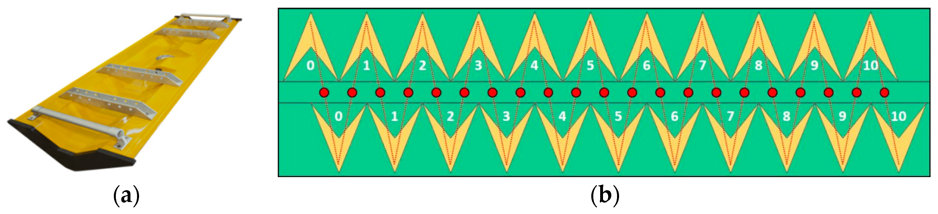
The GPR system that was employed in this research consisted of a three-dimensional (3D) Radar DX air launched antenna array (3D-Radar AS, Norway, Figure 1a), a step frequency radar that is composed of 11 transmitters and 11 receivers arranged to acquire 21 radar profiles, spaced by 7.5 cm, giving a total system physical width of approximately 1.8 m. While being physically separated, the system can be considered as a monostatic array, due to the limited offset between the transmitter and receiver pairs. The elements are oriented in a magnetic transverse mode and are arranged as shown in Figure 1b.
The main concept behind it is to obtain a large bandwidth that is pushed towards the lower end of the spectrum, maximising the trade-off between penetration and resolution. At shallow depths, the high frequencies are less attenuated; hence, it is useful to process the full bandwidth to obtain maximum resolution. However, using the same wide frequency span for larger depths will not be the optimum solution, since the high frequencies are attenuated below the noise level of the receiver. Thus, a full bandwidth processing will likely produce a noisy radargram at these depths, and therefore the lower frequencies are usually preferred. Such systems give the possibility of conjugating large bandwidth and low frequencies, which offer an optimum resolution as a function of depth of penetration [50,51].
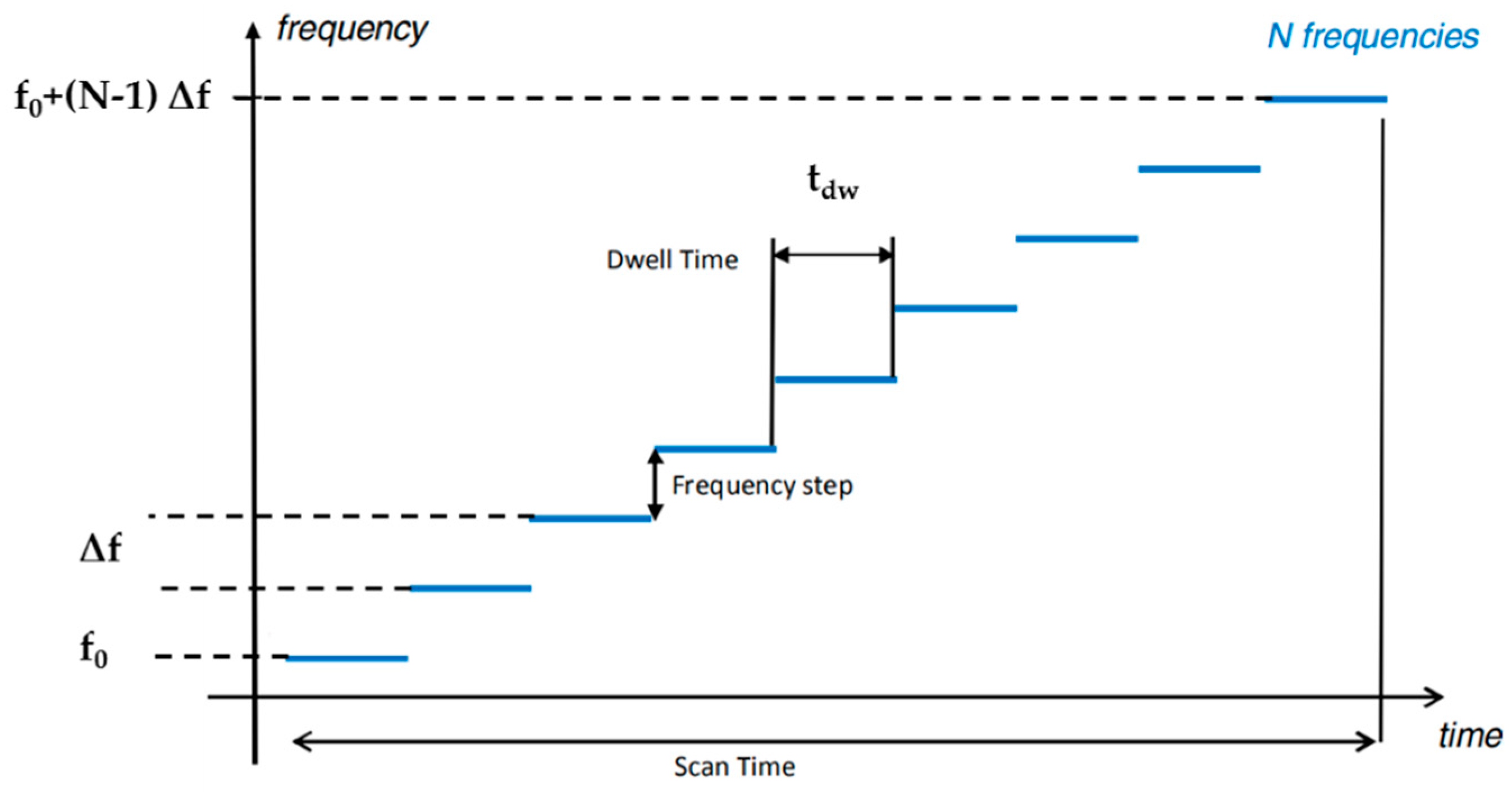
The emitted waveform consists of a train of sinewaves whose frequency linearly increases in discrete steps, as shown in Figure 2, where each step of the staircase corresponds to a sinewave with a specific frequency.
The fundamental parameters waveform parameters for a step-frequency GPR are: (1) the dwell time, representing the time that the system spends on a single frequency, (2) the frequency step, which is the increment in frequency between successive sinewaves, and (3) the number of frequency samples, defining, together with the frequency step, the effective bandwidth for the step-frequency waveform. These concepts are described by the following equations:
where is the minimum frequency, is the size of the frequency step, and N is the total number of sinewaves steps. The effective number of emitted sinewaves can be inferred by inverting Equation (2), which, for the described experimentations, corresponds to a total of 1401 frequencies.
Therefore, the recorded data represent the frequency response of the subsurface, and the time domain trace is obtained that sums over all the frequency components by the means of an inverse Fourier transform. Theoretically, the time-domain data that were retrieved from a step-frequency radar are equivalent to time-domain data from an impulse radar, but clearly the frequency data allows for a much wider range of frequency domain processing possibilities.
2.2. Experimental Campaign
A GPR survey was carried out in an agricultural field that was located in the near the CREA (Council for Agricultural Research and Economics) periferic operative structure in Treviglio (BG), Italy. The site is commonly used as a cornfield and it is characterised by relatively high organic matter content and soil moisture.
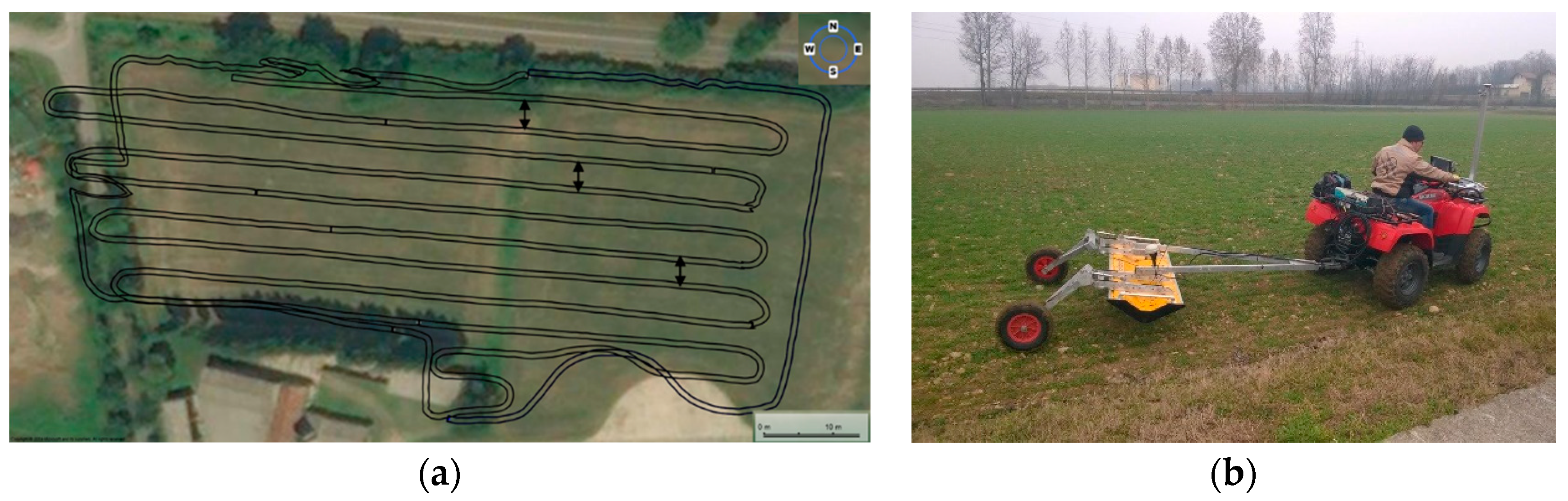
The antenna was mounted on a lightweight trailer that was pulled by a vehicle along each survey line, allowing for the acquisition of a series of roughly parallel profiles covering an area of 17,000 sqm at a speed of 3 km/h. Table 1 summarises the instrument acquisition parameters, while the profiles pattern and scanning platform are pictured in Figure 3.
3. Radar Results
3.1. GPR Data Processing and Slice Analysis
Time domain data was obtained by Inverse Fast Fourier Transform (IFFT), applying zero padding to the complex frequency domain data to calculate the time domain signals. No windowing functions have been applied to preserve the maximum achievable resolution and to avoid the possible corruption of the raw data; hence, the step-frequency GPR trade-off between the sharpness of the central lobe (resolution) and amplitude of the side lobes (ringing) of the pulse in the time domain has been met by weighting the achievable resolution. The only additional processing algorithms were in time alignment, to calibrate the time zero reflection, and an autoscaling function to adjust the saturation level.
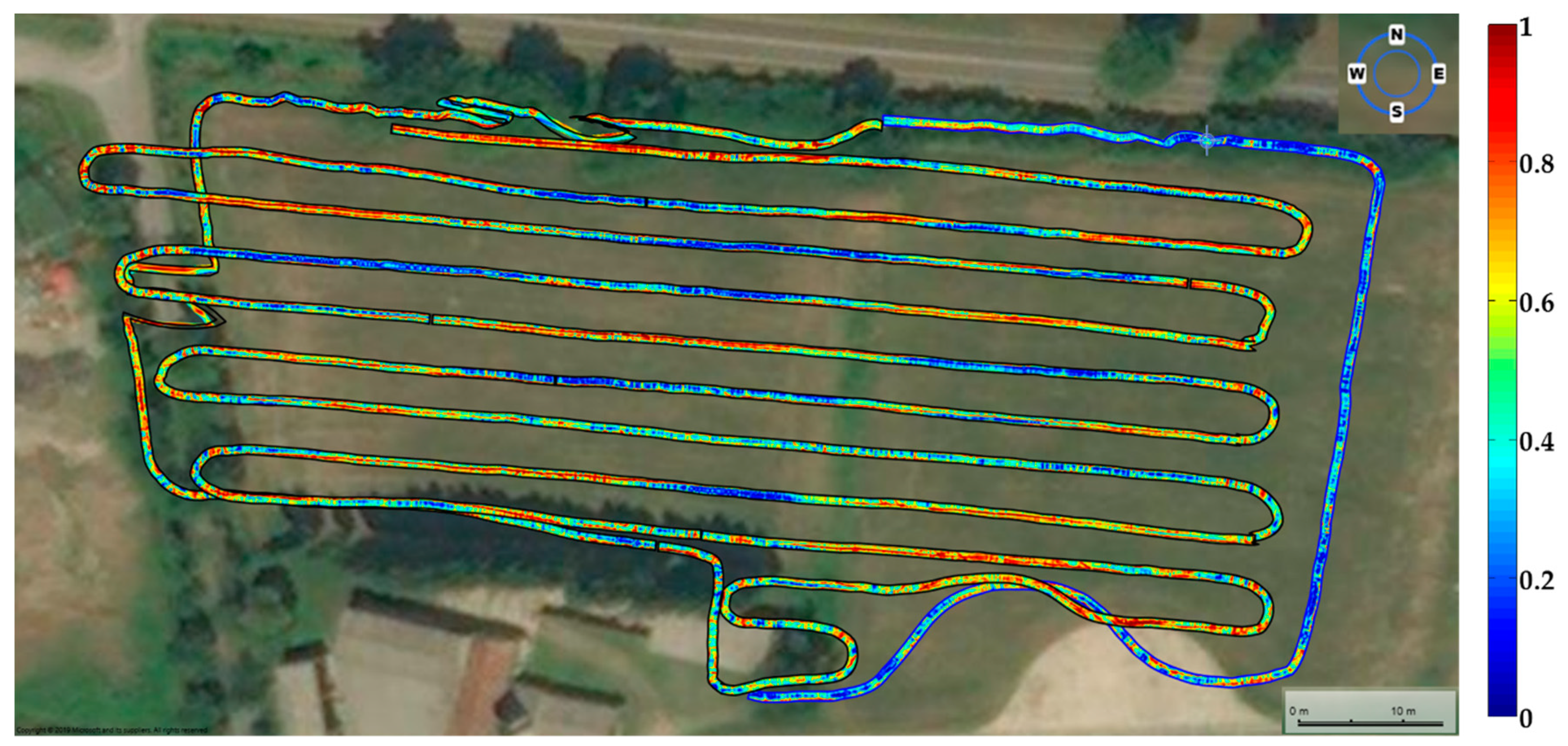
For descriptive purpose, Figure 4 presents a processed time slice for the full bandwidth located at 2.8 ns. Amplitude of the slice is displayed in the blue-yellow-red colourmap, in which the red values represent the pixels with higher amplitude
In general terms, it can be seen that the subsurface presents significant heterogeneous appearance, with several high amplitude areas (i.e., high permittivity) that are spread all over the acquired area, due to the properties and characteristics of the local subsurface conditions. A further note can be made when considering the straight segment that was located in the eastern sector of the image, which is located in an area of the field that has not been affected by possible land preparatory works. Along this profile, the radar results exhibit, to some extent, homogeneous, low amplitude behaviour, without any clear morphology or visible texture. Given such spatial heterogeneity, it could also be affirmed that the detection and identification of these features would have been hard to retrieve while employing the traditional geophysical methods.
When considering the well-known frequency-dependent behaviour of the possible components influencing the overall radar response and in order to highlight these features, the total bandwidth span has been divided into a number of narrow frequency bands by changing the size of the IFFT operator. In particular, a total number of 24 sub-bands have been isolated, which range from 300 MHz to 2700 MHz and spectrally spaced by 100 MHz. As a practical note, the employment of GPR equipment working in the frequency domain is fundamental for this kind of data analysis, as the signal generation technique ensures that those particular frequencies of interest are effectively present and they can be consistently isolated.
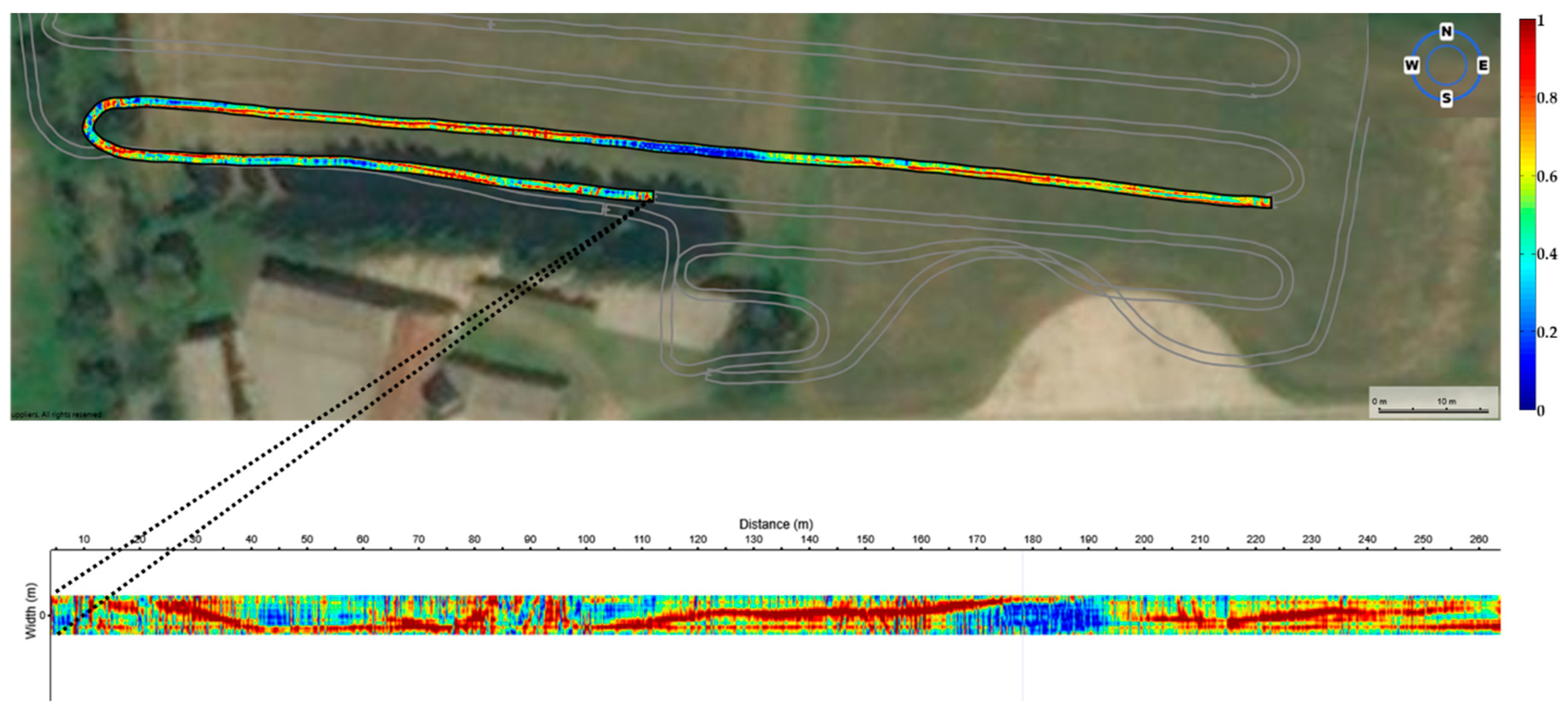
Among all of the acquired profiles, the one shown in Figure 5 has been taken as a reference for the results analysis.
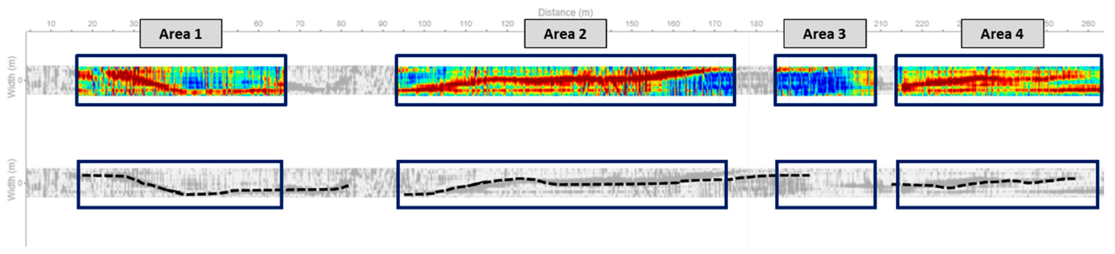
To allow for a detailed analysis, the profile has been split into a number of reduced segments, as shown in Figure 6, together with an interpretative sketch.
The selected profile exhibits a texture that is characterised by the presence of a number of structures (respectively, in Area 1, Area 2 and Area 4 of Figure 6) with a well-defined shape and with a high permittivity, along with areas where it is not possible to delineate a clear geometry of the visible morphology due to the absence of evidences of reflections (Area 3, except for the linear feature in the top-left part of the area that can be associated with the previous sector).
3.2. Frequency Analysis
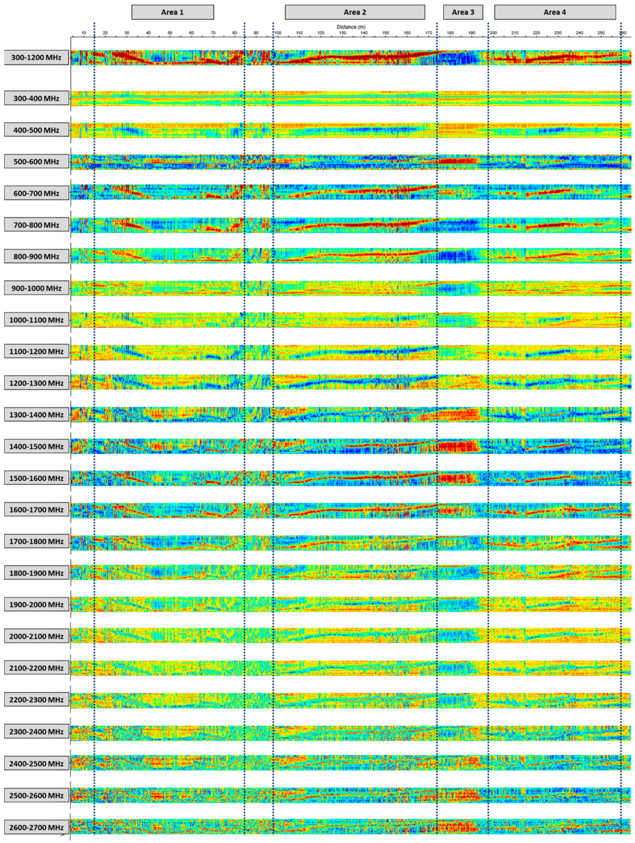
Figure 7 presents the magnitude values of the radar time slices ( ns) that were obtained from the above-mentioned frequency bands. Amplitude of the slices is displayed in the same blue-yellow-red colourmap adopted before and normalised by the overall maximum value to the range [0–1]. The full bandwidth result is included for a comparison purpose.
The visual inspection of the different slices demonstrates that the response of the highlighted events has a noticeable frequency dependent behaviour, and therefore the effective contribution to the overall signature that is produced by certain bands might be more relevant than others, as can be clearly seen by analysing the segment marked Area 3, which in the original data appears as a homogeneous, low amplitude area. The results suggest that the permittivity contrast is subjected to significant fluctuations as a function of frequency, as it can be noticed that the previously identified structures vanish and it becomes hard to delineate and extract them from the surrounding space at particular frequency intervals.
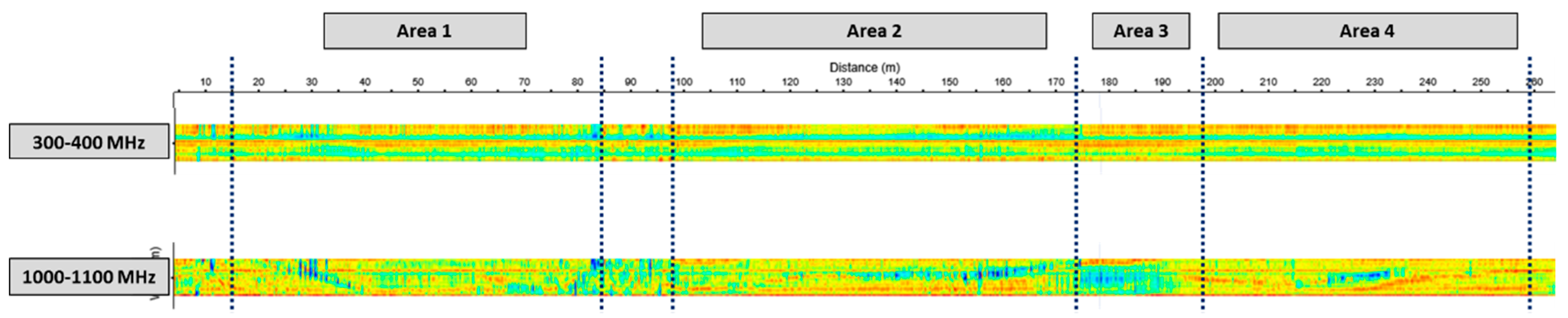
A preliminary analysis can be made regarding the useful or practical frequency boundaries. The low frequency components (up to 400 MHz) does not yield a significant informative content, both in terms of amplitude contrasts and clear definable structures. The profile in this frequency range appears roughly homogeneous, even though some slight amplitude variations can be detected. Even if a similar low amplitude appearance can be observed in other frequency bands (see, for example, the 900–1000 MHz band), the limited details that can be inferred by the slice are clear (Figure 8).
The choice of maintaining an equal bandwidth range for the entire ensemble of frequency intervals implies that the ambiguity in time remains unchanged, as the pulse duration does not change; however, increasing the central frequency of the signal brings an increased sensitivity of the system to the scattering phenomena, as they only occur when the size of the scatterer is comparable to or larger than the signal wavelength. Essentially, the vertical resolution is constant, but the minimum dimension of the detectable scattering object becomes smaller.
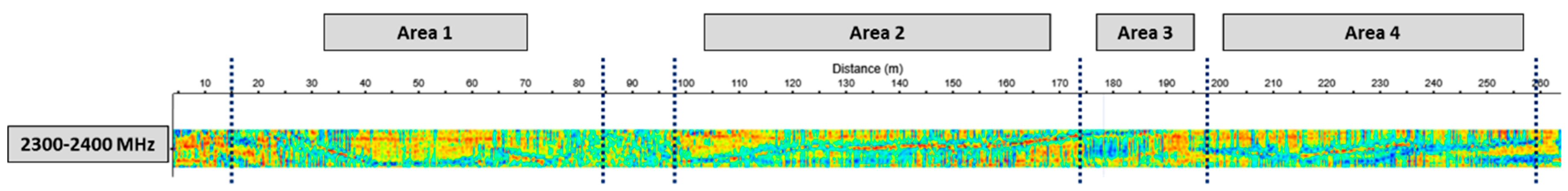
On the contrary, it can be stated that noise visibly starts to corrupt the data when the central frequency exceeds 2300 MHz, despite a shallow slice, which suggests high loss subsurface characteristics (Figure 9).
This last aspect is justifiable when considering that the survey was carried out during the winter season, in an area that was subjected to numerous rainfall events and characterised by a high degree of humidity.
Proceeding with a detailed characterisation of the different areas, further considerations can be developed, in particular, for what concerns the morphology and the texture of each sector.
From 400 MHz onward, a more detailed morphology smoothly appears, and the profile begins to show variations and differences, even if it can be said that the structures marked in Area 1, Area 2, and Area 4 gain a defined shape that starts from 600 MHz (Figure 10).
The texture maintains a well-defined contour for the entire frequency space, even if sharp fluctuations of the amplitude levels are evident, as previously highlighted. This concept is described in Figure 11, being focused on Area 2.
The only visible difference in the delineation performance of the linear feature is related to the increase of the central frequency, essentially for the previously described reasons. In this case, the enhancement of the scattering phenomena sensitivity produces a better defined slice, given a constant lateral resolution. This can be observed when considering, for example, the two intervals 700–800 MHz and 1500–1600 MHz, even though the effect is not as evident as expected due to the soil absorption.
The periodicity of the amplitude fluctuations describes a trend in which the permittivity contrast of the structured feature is alternatively higher or lower than the one of the enclosing space, including scenarios in which the contrast in permittivity approaches zero, as for the 900–1000 MHz frequency interval, which proves the significance of the information generated by the analysis. Visibly, this situation does not impact the image generated from the full bandwidth analysis, but it does play a role if the objective is to lately retrieve information regarding the soil properties.
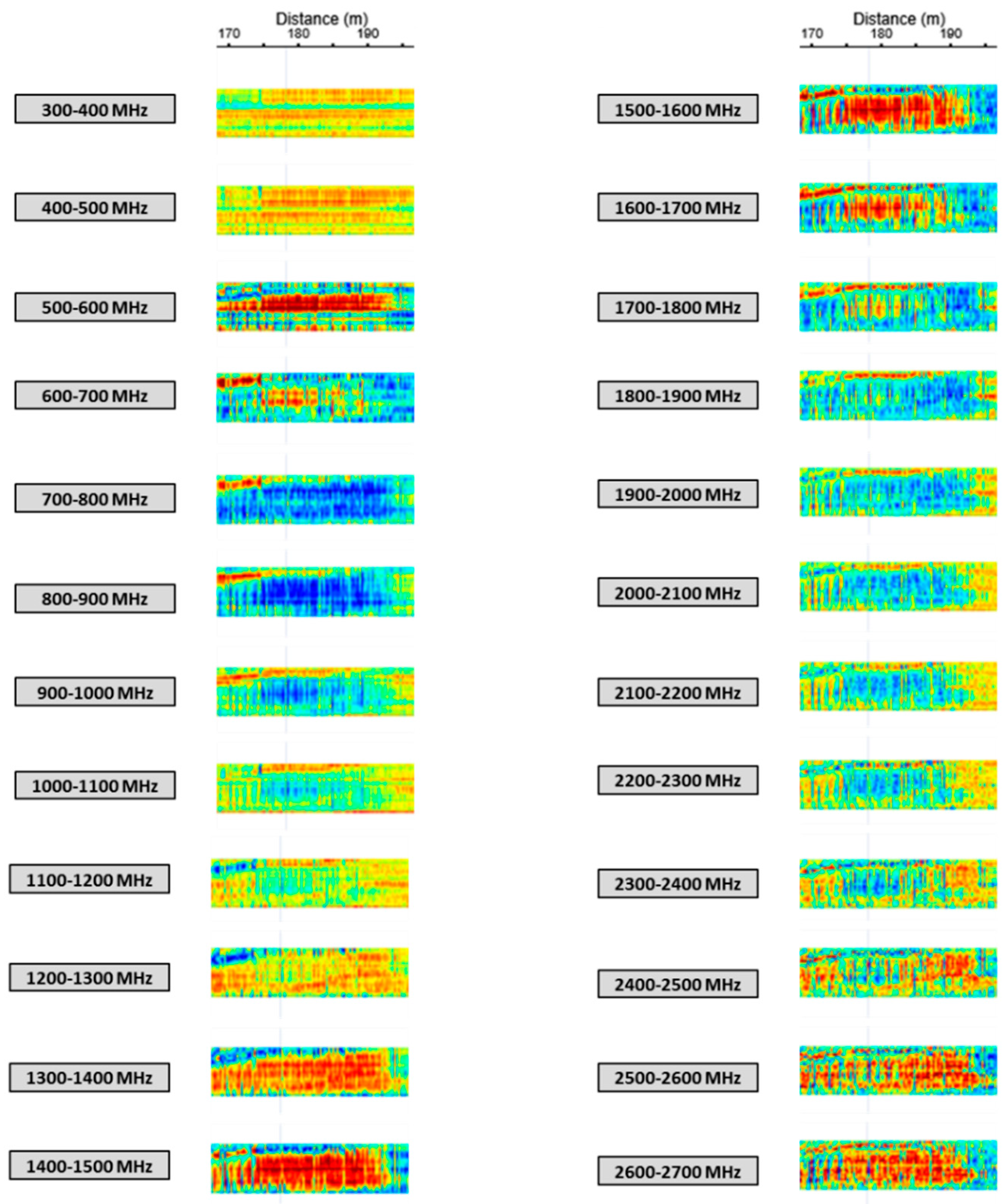
Finally, Area 3 oddly presents only a defined texture in the 500–600 MHz band, in this case not geometrically belonging to the previous sector and not occurring elsewhere, while no evidences of structured reflection are detectable, as inferred by the full bandwidth analysis of Figure 7. Figure 12 presents the slices.
Conversely to what has been inferred and supposed from the full bandwidth analysis, the linear feature that is located in the top-left part of the slices does not exhibit a coherent behaviour with the adjacent area, as (1) it does not appear in the same frequency range, but approximately at 1000 MHz and (2) its amplitude variations with frequency are, at the same time, not consistent with the patterns tracked by Area 2 and Area 4. Figure 13 visualises these considerations.
It is evident that the continuity observable from 300–2700 MHz slice is not confirmed when the slice is analysed in narrower frequency sub-bands, thus demonstrating the increased level of information that the developed approach can reach once again.
4. Results Discussion
Some statistical measures have been computed and evaluated for each of the defined areas to qualitatively highlight the frequency-dependent imaging results.
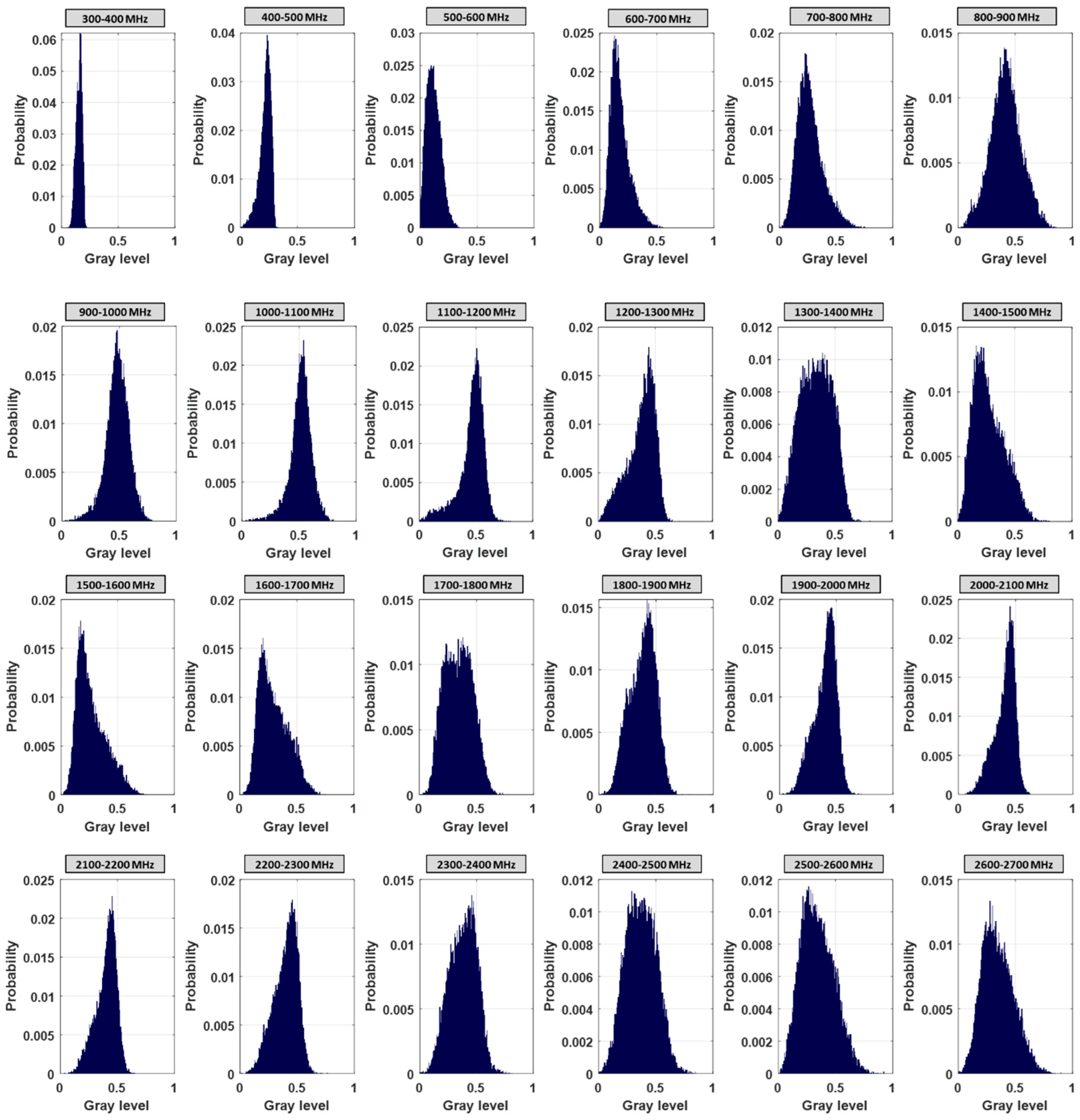
The differences are clear when analysing the histogram of the image (Figure 14), which shows the number of pixels in an image at each different intensity value. Obviously, the histogram represents a reduction of the dimensionality (i.e., it contains no spatial information) relative to the original image, therefore it cannot be deduced form the histograms visualisation, but this feature provides information regarding the relative positions of various grey levels within the image and indirectly on its texture [52,53].
When considering that, in a GPR image, the amplitude levels (pseudo-colour) are closely related to the contrast in the electrical properties, for a frequency-independent scenario no significant variations would have been expected among the amplitude distributions, while what can be noticed in Figure 13 represents a completely different situation. In particular, it can be seen that, what has been described in Figure 8 reflects in its correspondent histogram, as the sharp shape of the distribution (y-axis) defines an image, in which there are a limited number of amplitude levels (i.e., nearly a uniform image) that are concentrated on a limited interval (i.e., low amplitude, x-axis). The behaviour in the different frequency intervals can be summarised as a recurrent increase and a decrease of the number of amplitude levels, which are visible as a contraction of the width of the histogram, while the hint of the periodicity can be inferred by the location (right-side or left-side) of the histogram slope. Clearly, the heterogeneity of the slice prevents a significant shift in the location of the histogram.
Generally, two main features can be extracted from Figure 14: (1) the shape of the histogram represents the number of different amplitude levels in the image, defining whether the image is homogeneous or not, while (2) its location provides an indication of the amplitude of the image pixels.
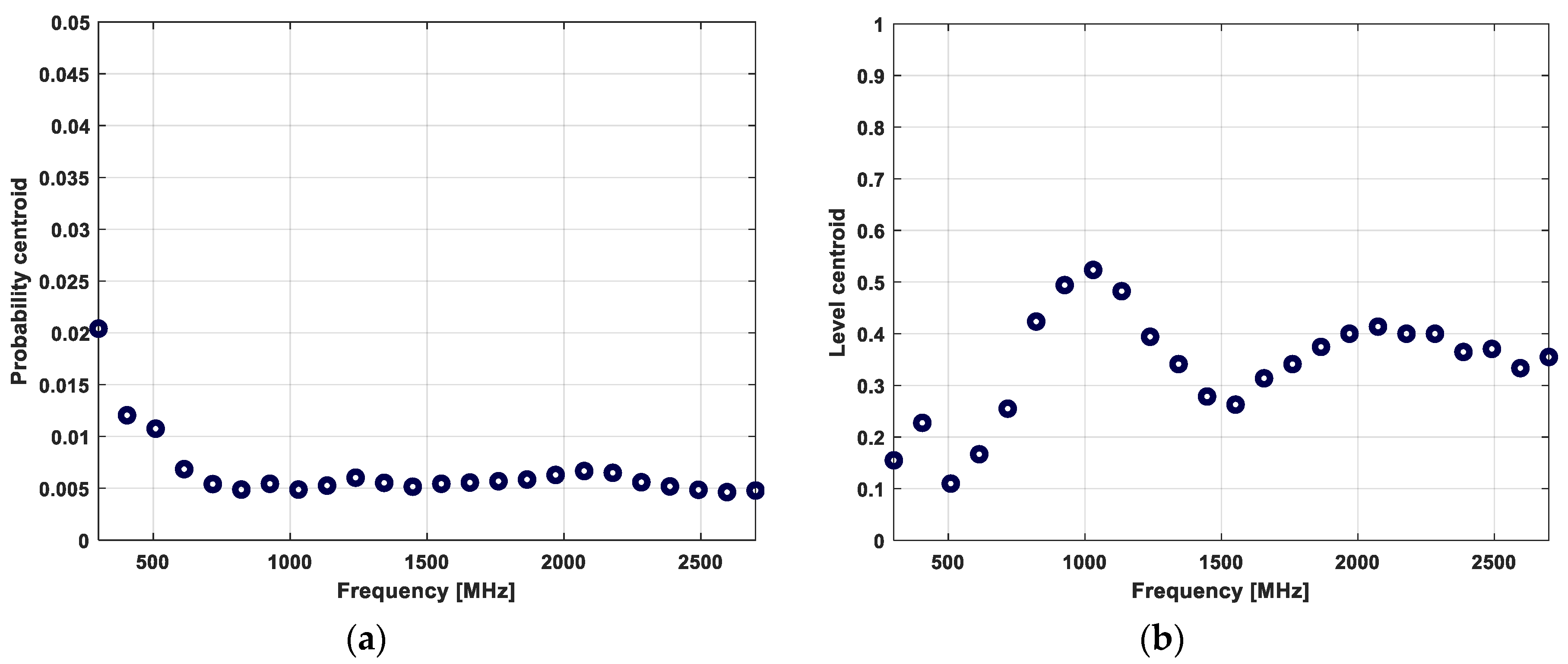
Tracking the centroid of the histograms, as plotted in Figure 15 against the frequency interval, can also highlight the variations.
This feature represents the centre of mass of each histogram plotted in Figure 14, and it can essentially be considered as a summary of the information that can be extracted from it, which shows the frequency-dependent variations of the different pixel levels occurrence, as shown in Figure 15a as the level probability, and the amplitude level at which it occurs, as depicted in Figure 15b as the level centroid. Following the considerations that were outlined before, the characteristics of the 300–400 MHz slice can be inferred while considering that (1) a high probability (Figure 15a, y-axis) means that the number of different pixel levels is limited and (2) these levels are primarily distributed at lower values (Figure 15b, y-axis). These two characteristics suggest a homogeneous image, in which only few amplitude levels contribute to the total image appearance.
Obviously, when the slice becomes more composite, the probability centroid loses its significance, as the increase in the number of the different levels brings a reduction in their probability of occurrence, which produces an approximately stable centroid. The location of these occurrences is what gains relevance (Figure 15b). In particular, the hypothesis that was made on the periodicity of the frequency-dependent variations can be clearly visualised while looking at the oscillation that was described by the pattern of the level centroid. If one considers the relationship between the pixel amplitude and the associated GPR effect, these variations highlight that the amplitude content of each slice alternatively varies from a prevalence of high contrast regions to slices in which there are less variations.
Following these considerations, the peak visible at a frequency of 1000 MHz and located approximately at 0.5, which means that there is not a clear prevalence of low/high amplitude levels, reflects the appearance of the corresponding slice of Figure 7. The sharpness of the pattern decreases with the increasing frequency intervals due to the noise contribution: as the metric is not sensitive to the geometrical features that are included in the slice, the effect of noise is to spread the number of pixel amplitude levels, therefore the x-axis of the histogram centroid also becomes more stable with frequency.
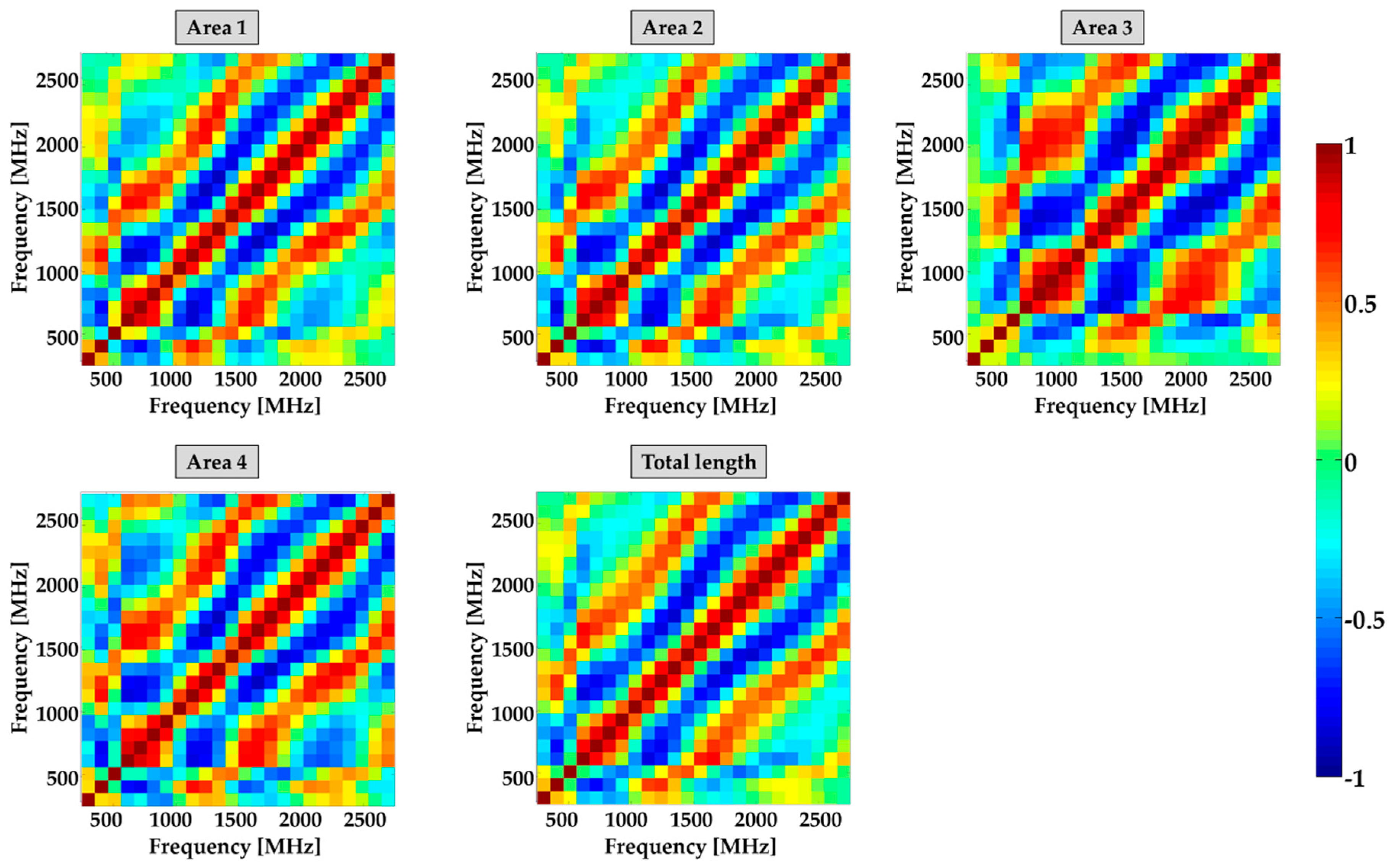
This regular alternation can also be observed from the pattern that was described by the maximum and minimum values for all the defined areas, and it is clearly identifiable by analysing the results of the correlation analysis [54,55], computed while isolating each single area and considering the total profile length (Figure 16).
The correlation matrix, as defined in (1), has been computed for each pairwise profile combination (, ), on the mean-adjusted (, ) and standard deviation normalised (, ) profiles.
In which represents the Pearson coefficient, as calculated in (2)
The correlation coefficient has the value if the two images are absolutely identical, if they are completely uncorrelated, and if they are completely anti-correlated, for example, if one image is the negative of the other. One of the obvious advantages of the Pearson’s correlation coefficient is that it condenses the comparison of different two-dimensional images down to a single scalar, and it is completely invariant to linear transformations of the images. As a result, is insensitive (within limits) to uniform variations in brightness or contrast across an image.
The values that are shown in the correlation matrix are a measure of the similarity that occurs between each pairwise frequency combination. In particular, a correlation close to 1 means that the two particular slices are highly related, hence the two resulting frequency behaviours (i.e., material response to the frequency variation) are similar. Performing a pixel by pixel comparison, the computed coefficients take into account, not only the amplitude values, but also their distribution, and consequently the geometrical features of the image.
It is evident from the results that these frequency dependent fluctuations occur, regardless of the presence of a defined morphology and with a highly similar pattern. Further on, the dynamic range of the coefficients spread from −1 to 1, meaning that there are situations in which the resulting slices might be perfectly uncorrelated, while the periodicity effects can be inferred by the frequency intervals in which the slices are perfectly negative correlated (the two quantities move in opposite direction).
Table 2 provides a comparison that is based on an average and standard deviation of the correlation coefficients for each of the situations that are presented in Figure 16.
Although being basic statistical descriptors, these two values are a convenient instrument in comparing the consistency of the results. The values in the table summarise what has been commented, and while the low average value is affected by the heterogeneity of the particular area, the deviation of the correlation coefficients reflects their maximum fluctuation; therefore, it is a significant descriptor in evaluating the magnitude of these response variations over the frequency space. In particular, a correlation deviation of 0.5 means that the coefficients may vary from describing a totally uncorrelated slice () to a closely comparable one (positive or negative as well).
However, it can be also noted from Figure 16 that each of the marked area has its own variations pattern, therefore the assumed periodicity does not exactly replicate itself exactly when changing the local subsurface properties and the investigated frequency band.
What has been highlighted can be numerically confirmed while computing the second order correlation (correlation between correlation), whose values are listed in Table 3.
Two main considerations can be pointed out from Table 3:
- High similarity exists among the correlation results of Area 1, Area 2, and Area 4, which suggests a close correspondence of the soil properties of those areas (given the similar pattern).
- The correlation values of Area 3 are significantly lower (almost a half), with the outcome that can result from both the different morphology of the area and a variation in the frequency response of the soil characteristics.
The reduced correspondence between the correlation that was obtained when considering the profile total length and the one of Area 3 (and conversely the high values compared to Area 1, Area 2, and Area 4) is a consequence of this mutual behaviour, as clearly presence of a higher number of areas with a coherent behaviour mainly govern the first order correlation.
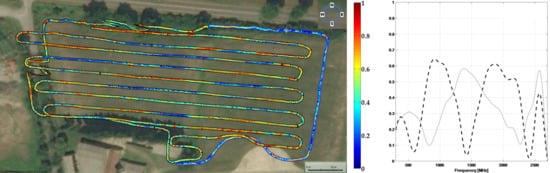
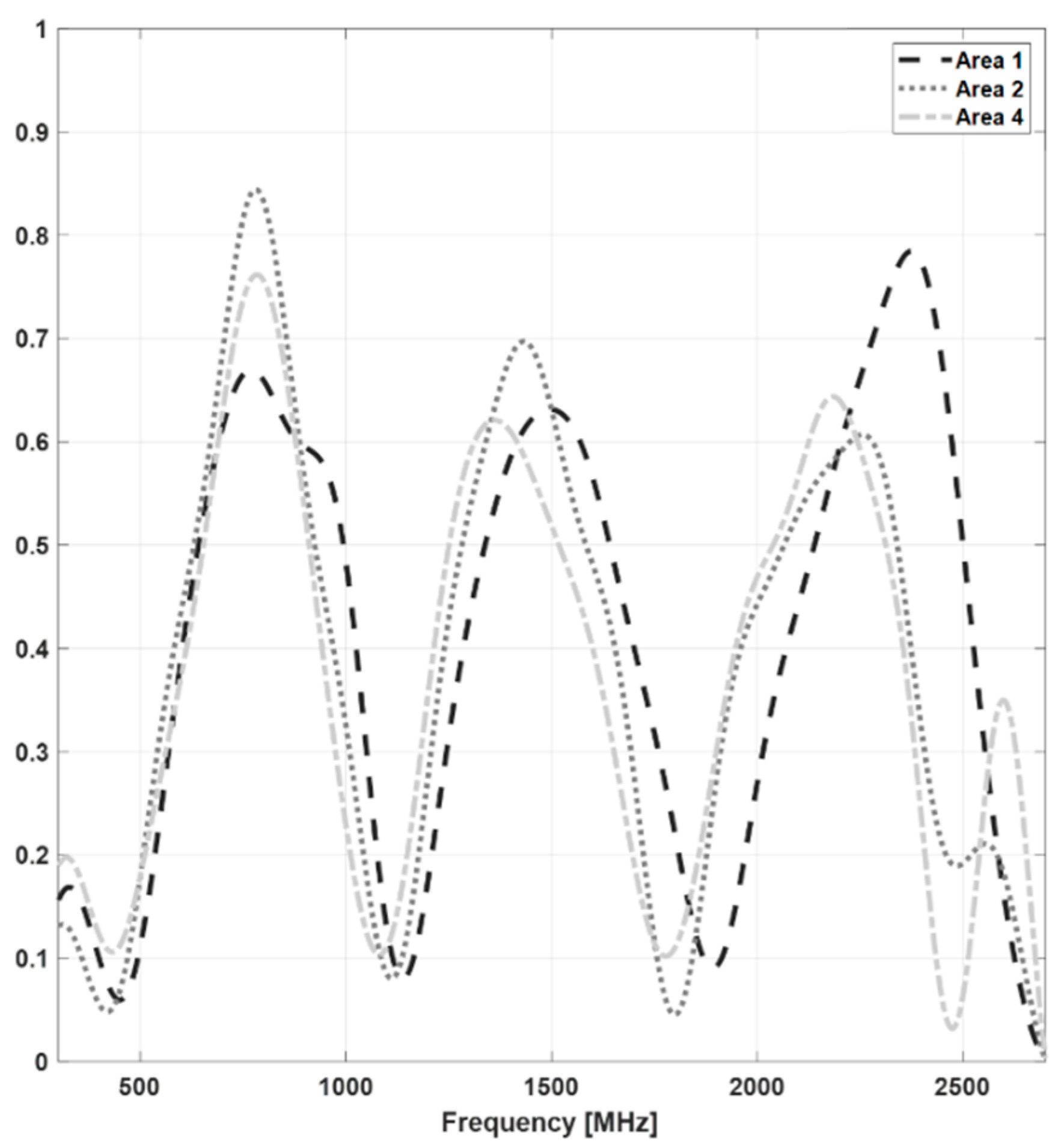
The fact that the geometrical properties remain uniform suggests that the changes in the response of the feature with the frequency are likely to be caused by the local subsurface constituents. In addition, while taking into account the highly correlated trend of the amplitude variations over the frequency space for Area 1, Area 2, and Area 4, it can be supposed that the three segments are a part of the same extended feature, which act as a unique structure and hence possess the same electrical properties. Figure 17 provides a demonstration of this hypothesis, in which the amplitude of the marked structure is plotted against the frequency interval for all three areas.
The three amplitude patterns are highly comparable, both observing the dynamic range of the amplitude values and the periodicity of the peaks. The differences are visible in the higher part of the spectrum, even though it should take into account the high noise level that might affect the amplitude results. What can be further noted is that, despite the increase in the central frequency, the amplitude response of the feature remains almost unchanged.
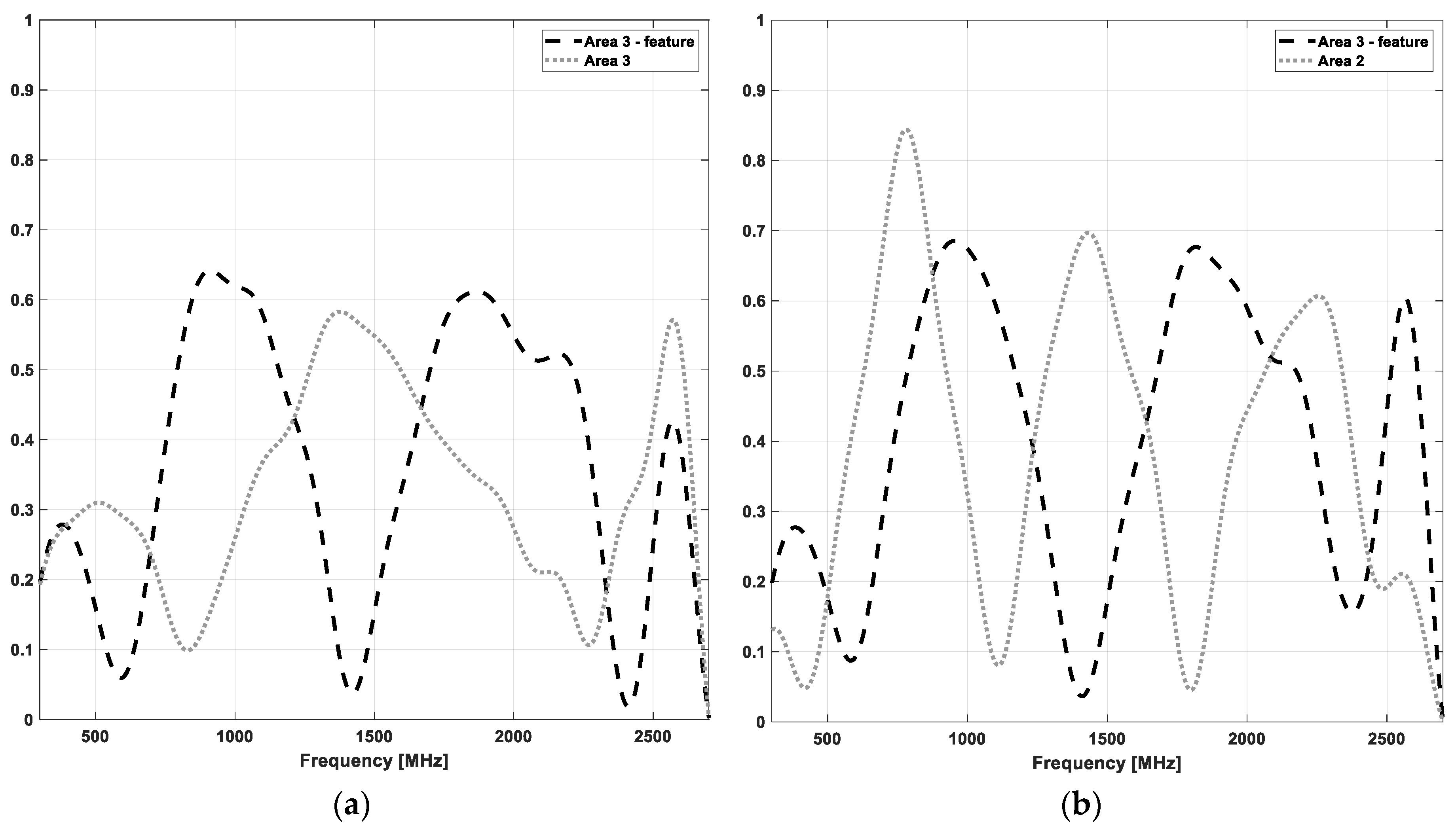
Figure 18 provides a amplitude pattern comparison.
The fact that the highlighted segment does not reflect either of those behaviours can be explained as the result of a feature that morphologically belongs to the previous area, but is located in an area that possesses different electromagnetic properties. Clearly, this complex interaction does not appear in the full bandwidth results, which once again demonstrates the valuable information that can be extracted by a frequency analysis of the GPR data.
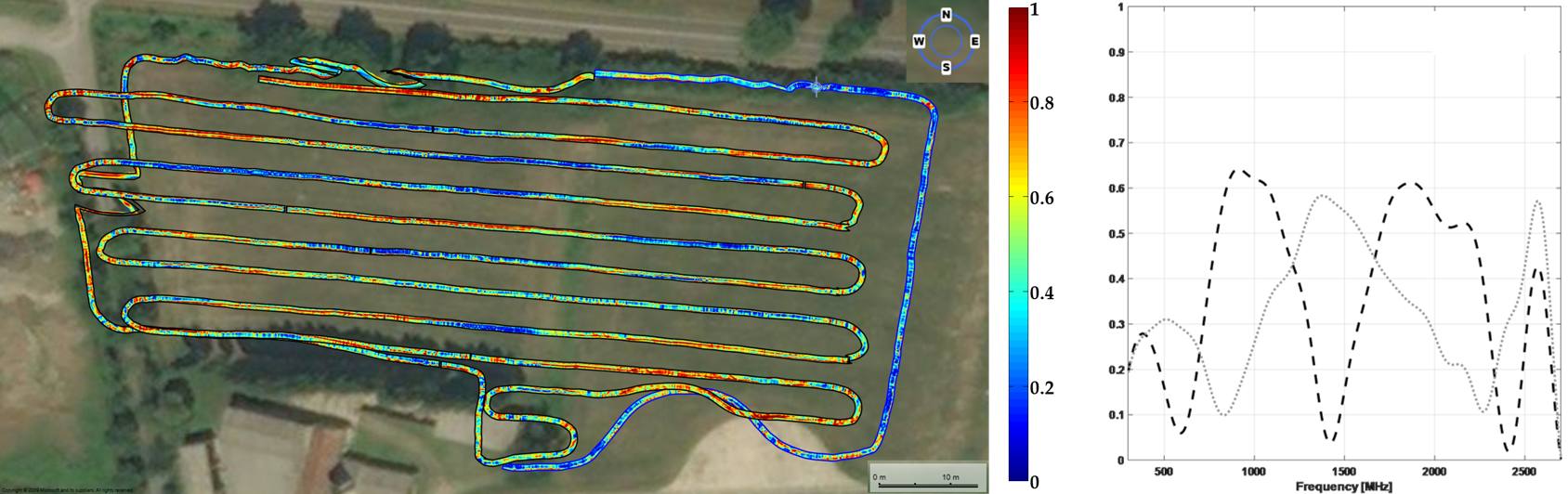
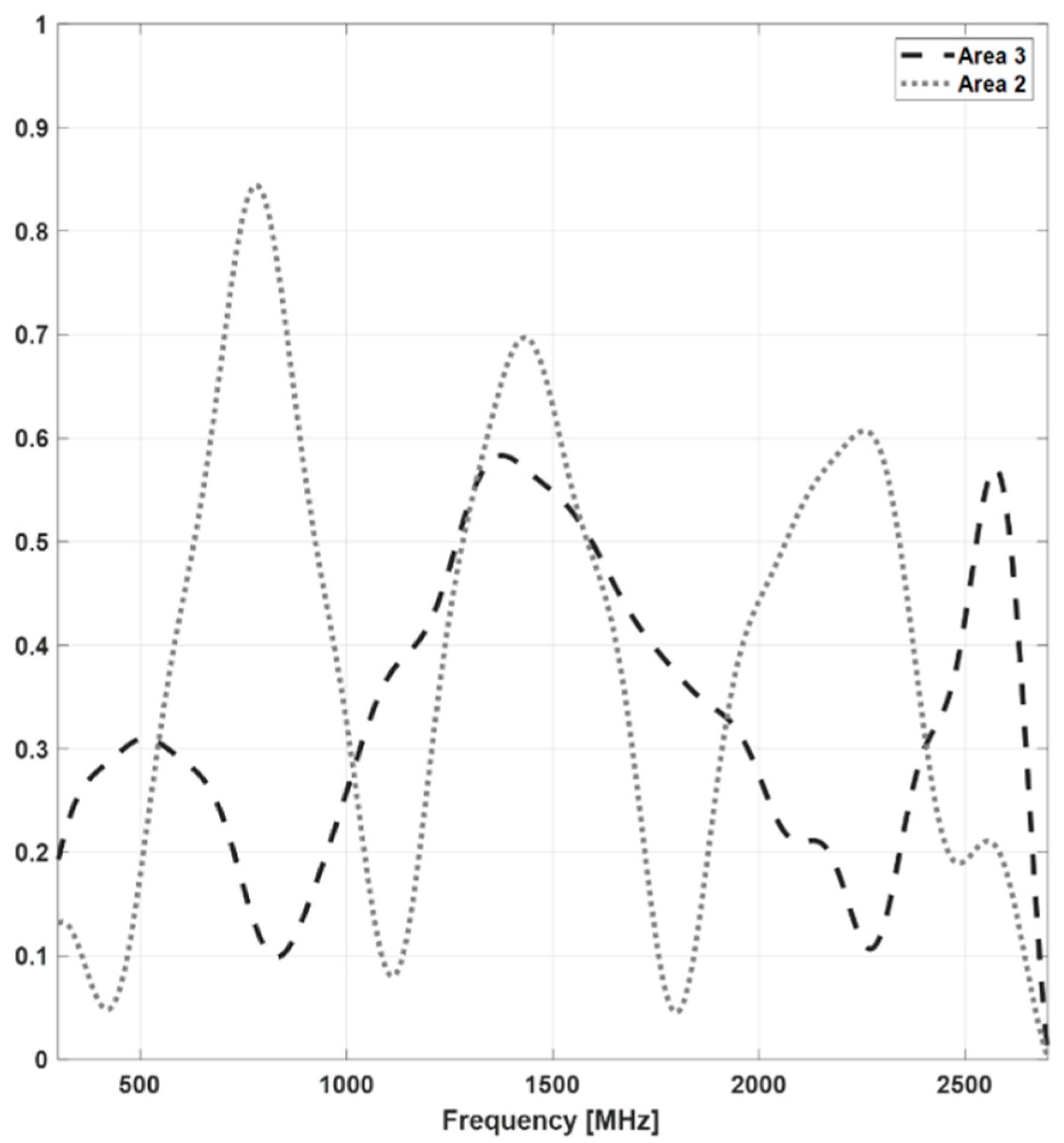
This can be easily seen by comparing the outline designed by the amplitude variations of Area 2 and Area 3, as shown in Figure 19.
What can be noticed is that, not only the occurrence of the peaks does not match, but also the periodicity of the amplitude variations is different. Moreover, the periodicity is not regular, as (1) the first peak of Area 2 (located near 800 MHz) corresponds to a minimum of Area 3, (2) the second peak of Area 3 (at 1400 MHz) roughly corresponds to the one identified for Area 2, and (3) the last peak of Area 2 considerably precedes its corresponding one. These results might indicate a heterogeneous change in the soil electrical properties.
As a comparison, a similar trend has been found in previous work that characterises soil properties in the frequency domain. In particular, even if no direct comparison can be made, what can be confirmed is that (1) the response of the subsurface in the frequency domain is characterised by an oscillatory behaviour and it is highly nonlinear [56,57], (2) the occurrence of the local minima and maxima of the response function depends on the constitutive parameters of the soil, as can be seen in the results from [58,59], in which, respectively, a change in the clay content and moisture of the soil sample is evaluated.
5. Conclusions
The measured values of electrical properties reveal the heterogeneity of soil that is present in a single agricultural field and are affected by a number of physical soil characteristics, which are of significant importance in precision agriculture.
In this framework, GPR has proven to be an effective tool for efficiently measuring soil properties that achieve, at the same time, a suitable resolution and large scale measurements, a demanding requirement due to the three-dimensional distributions of the physical characteristics beneath most agricultural terrains and their variability. GPR methodology is based on the fact that soil permittivity is affected by more than one important physical soil characteristic, where behaviour is frequency dependent to some extent. In the agricultural field, the subsurface interactions can be very complex and, as the GPR transmitted pulses are modified at multiple frequencies, the received signals carry influences from various sources.
In this study, a SFCW GPR has been employed for highlighting these frequency dependency behaviours in order to show what can be gained by analysing the radar response through a series of narrow bandwidth, rather processing the entire available bandwidth.
The paper has demonstrated that, in comparison to the full bandwidth result, the frequency analysis is able to retrieve the intricate and often indiscernible textural variability that is found within a complex GPR image that help to delineate the regions of similar soil characteristics. The fundamental reason is that the highlighted frequency effects exhibit relevant amplitude variations, a feature that will presumably be lost when integrating all of these different frequency contributions in a single time domain signal. Additionally, this strategy allows for a qualitative characterisation of the subsurface electrical properties overcoming the need for a known subsurface reflector.
In particular, evaluating and mutually correlating the amplitude fluctuations with frequency make it easier to identify the subsurface features that are possibly correlated or conversely possessing different electrical properties, providing substantial improvements in the process of soil morphology characterisation.
Following the presented qualitative evaluation, prospective activities will focus on the quantitative analysis of the results, which is the translation of the apparent permittivity contrast into the physical parameters that are responsible for these radar response variations. This can be achieved by clustering the different GPR volumes depending on their frequency behaviours and by comparing them to the theoretically expected variations, while considering that unique and unambiguous relationships might be a challenging task due to the heterogeneity of the soil composition (texture, moisture, and organic matter content). More robust classification and recognition can be obtained when comparing the results with other related methodologies and through the available a priori information on the area.
Author Contributions
Conceptualization, F.L. and M.L.; methodology, F.L.; data processing, F.L.; data analysis, F.L. and M.L.; writing—original draft preparation, F.L.; writing—review and editing, M.L.; supervision, M.L.; project administration, M.L.
Funding
This research was funded by Regione Lombardia, under project “AgriGeoH2O”—grant number 145427. The APC was funded by Politecnico di Milano, Milan, Italy.
Acknowledgments
Authors are grateful to CREA Council for the availability of the test field.
Conflicts of Interest
The authors declare no conflict of interest.
References
- Cho, S.E. Effects of spatial variability of soil properties on slope stability. Eng. Geol. 2007, 92, 97–109. [Google Scholar] [CrossRef]
- Usowicz, B.; Lipiec, J. Spatial variability of soil properties and cereal yield in a cultivated field on sandy soil. Soil Tillage Res. 2017, 174, 241–250. [Google Scholar] [CrossRef]
- Unamunzaga, O.; Besga, G.; Castellón, A.; Usón, M.A.; Chéry, P.; Gallejones, P.; Aizpurua, A. Spatial and vertical analysis of soil properties in a Mediterranean vineyard soil. Soil Use Manag. 2014, 30, 285–296. [Google Scholar] [CrossRef]
- Brevik, E.C.; Calzolari, C.; Miller, B.A.; Pereira, P.; Kabala, C.; Baumgarten, A.; Jordán, A. Soil mapping, classification, and pedologic modeling: History and future directions. Geoderma 2016, 264, 256–274. [Google Scholar] [CrossRef]
- Rossel, R.V.; Adamchuk, V.I.; Sudduth, K.A.; McKenzie, N.J.; Lobsey, C. Proximal soil sensing: An effective approach for soil measurements in space and time. In Advances in Agronomy, 1st ed.; Springer: Amsterdam, The Netherlands, 2010. [Google Scholar]
- Allred, B.; Daniels, J.J.; Ehsani, M.R. Handbook of Agricultural Geophysics, 1st ed.; CRC Press: Boca Raton, FL, USA, 2008. [Google Scholar]
- Steeples, D.W. Engineering and environmental geophysics at the millennium. Geophysics 2001, 66, 31–35. [Google Scholar] [CrossRef] [Green Version]
- Adamchuk, V.I.; Hummel, J.W.; Morgan, M.T.; Upadhyaya, S.K. On-the-go soil sensors for precision agriculture. Comput. Electron. Agric. 2004, 44, 71–91. [Google Scholar] [CrossRef] [Green Version]
- Piikki, K.; Wetterlind, J.; Söderström, M.; Stenberg, B. Three-dimensional digital soil mapping of agricultural fields by integration of multiple proximal sensor data obtained from different sensing methods. Precis. Agric. 2015, 16, 29. [Google Scholar] [CrossRef]
- Candiago, S.; Remondino, F.; De Giglio, M.; Dubbini, M.; Gattelli, M. Evaluating multispectral images and vegetation indices for precision farming applications from UAV images. Remote Sens. 2015, 7, 4026–4047. [Google Scholar] [CrossRef]
- Ciampalini, A.; André, F.; Garfagnoli, F.; Grandjean, G.; Lambot, S.; Chiarantini, L.; Moretti, S. Improved estimation of soil clay content by the fusion of remote hyperspectral and proximal geophysical sensing. J. Appl. Geophys. 2015, 116, 135–145. [Google Scholar] [CrossRef]
- Castrignanò, A.; Buttafuoco, G.; Quarto, R.; Vitti, C.; Langella, G.; Terribile, F.; Venezia, A. A combined approach of sensor data fusion and multivariate geostatistics for delineation of homogeneous zones in an agricultural field. Sensors 2017, 17, 2794. [Google Scholar] [CrossRef]
- Sharma, L.K.; Bu, H.; Franzen, D.W.; Denton, A. Use of corn height measured with an acoustic sensor improves yield estimation with ground based active optical sensors. Comput. Electron. Agric. 2016, 124, 254–262. [Google Scholar] [CrossRef] [Green Version]
- De Benedetto, D.; Castrignanò, A.; Rinaldi, M.; Ruggieri, S.; Santoro, F.; Figorito, B.; Gualano, S.; Diacono, M.; Tamborrino, R. An approach for delineating homogeneous zones by using multi-sensor data. Geoderma 2013, 199, 117–127. [Google Scholar] [CrossRef]
- Agapiou, A.; Lysandrou, V.; Hadjimitsis, D. Optical remote sensing potentials for looting detection. Geosciences 2017, 7, 98. [Google Scholar] [CrossRef]
- Minet, J.; Lambot, S.; Delaide, G.; Huisman, J.A.; Vereecken, H.; Vanclooster, M. A generalized frequency domain reflectometry modeling technique for soil electrical properties determination. Vadose Zone J. 2010, 9, 1063–1072. [Google Scholar] [CrossRef]
- Pastuszka, T.; Krzyszczak, J.; Sławiński, C.; Lamorski, K. Effect of time-domain reflectometry probe location on soil moisture measurement during wetting and drying processes. Measurement 2014, 49, 182–186. [Google Scholar] [CrossRef]
- Davis, J.L.; Annan, A.P. Ground Penetrating Radar for high resolution mapping of soil and rock stratigraphy. Geophys. Prosp. 1989, 37, 531–551. [Google Scholar] [CrossRef]
- Lualdi, M.; Lombardi, F. Utilities detection through the sum of orthogonal polarization in 3D georadar surveys. Near Surf. Geophys. 2015, 13, 73–81. [Google Scholar] [CrossRef]
- Lai, W.W.L.; Dérobert, X.; Annan, P. A review of Ground Penetrating Radar application in civil engineering: A 30-year journey from Locating and Testing to Imaging and Diagnosis. NDT E Int. 2018, 96, 58–78. [Google Scholar] [CrossRef]
- Daniels, D.J. Ground Penetrating Radar, 2nd ed.; The Institution of Electrical Engineers: London, UK, 2004. [Google Scholar] [CrossRef]
- Ardekani, M.R.M. Off-and on-ground GPR techniques for field-scale soil moisture mapping. Geoderma 2013, 200, 55–66. [Google Scholar] [CrossRef]
- Zhang, J.; Lin, H.; Doolittle, J. Soil layering and preferential flow impacts on seasonal changes of GPR signals in two contrasting soils. Geoderma 2014, 213, 560–569. [Google Scholar] [CrossRef]
- Moghadas, D.; Jadoon, K.Z.; Vanderborght, J.; Lambot, S.; Vereecken, H. Estimation of the near surface soil water content during evaporation using air-launched ground-penetrating radar. Near Surf. Geophys. 2014, 12, 623–633. [Google Scholar] [CrossRef]
- Busch, S.; Van der Kruk, J.; Vereecken, H. Improved characterization of fine-texture soils using on-ground GPR full-waveform inversion. IEEE Trans. Geosci. Remote Sens. 2014, 52, 3947–3958. [Google Scholar] [CrossRef]
- Wang, P.; Hu, Z.; Zhao, Y.; Li, X. Experimental study of soil compaction effects on GPR signals. J. Appl. Geophys. 2016, 126, 128–137. [Google Scholar] [CrossRef]
- Tran, A.P.; Vanclooster, M.; Zupanski, M.; Lambot, S. Joint estimation of soil moisture profile and hydraulic parameters by ground-penetrating radar data assimilation with maximum likelihood ensemble filter. Water Resour. Res. 2014, 50, 3131–3146. [Google Scholar] [CrossRef] [Green Version]
- De Benedetto, D.; Castrignano, A.; Sollitto, D.; Modugno, F.; Buttafuoco, G.; lo Papa, G. Integrating geophysical and geostatistical techniques to map the spatial variation of clay. Geoderma 2012, 171, 53–63. [Google Scholar] [CrossRef]
- Topp, G.C.; Davis, J.L.; Annan, A.P. Electromagnetic determination of soil water content: Measurements in coaxial transmission lines. Water Resour. Res. 1980, 16, 574–582. [Google Scholar] [CrossRef]
- Benedetto, A.; Tosti, F.; Ortuani, B.; Giudici, M.; Mele, M. Mapping the spatial variation of soil moisture at the large scale using GPR for pavement applications. Near Surf. Geophys. 2015, 13, 269–278. [Google Scholar] [CrossRef]
- Huisman, J.; Sperl, C.; Bouten, W.; Verstraten, J. Soil water content measurements at different scales: Accuracy of time domain reflectometry and ground penetrating radar. J. Hydrol. 2001, 245, 48–58. [Google Scholar] [CrossRef]
- Bradford, J.H.; Harper, J.T.; Brown, J. Complex dielectric permittivity measurements from ground-penetrating radar data to estimate snow liquid water content in the pendular regime. Water Resour. Res. 2009, 45. [Google Scholar] [CrossRef] [Green Version]
- Garambois, S.; Sénéchal, P.; Perroud, H. On the use of combined geophysical methods to assess water content and water conductivity of near-surface formations. J. Hydrol. 2002, 259, 32–48. [Google Scholar] [CrossRef]
- Tillard, S.; Dubois, J.C. Analysis of GPR data: Wave propagation velocity determination. J. Appl. Geophys. 1995, 33, 77–91. [Google Scholar] [CrossRef]
- Comite, D.; Galli, A.; Lauro, S.E.; Mattei, E.; Pettinelli, E. Analysis of GPR early-time signal features for the evaluation of soil permittivity through numerical and experimental surveys. IEEE J. Sel. Top. Appl. Earth Obs. Remote Sens. 2016, 9, 178–187. [Google Scholar] [CrossRef]
- Algeo, J.; Van Dam, R.L.; Slater, L. Early-time GPR: A method to monitor spatial variations in soil water content during irrigation in clay soils. Vadose Zone J. 2016, 15, 11. [Google Scholar] [CrossRef]
- Algeo, J.; Slater, L.; Binley, A.; Van Dam, R.L.; Watts, C. A Comparison of Ground-Penetrating Radar Early-Time Signal Approaches for Mapping Changes in Shallow Soil Water Content. Vadose Zone J. 2018, 17, 11. [Google Scholar] [CrossRef]
- Olhoeft, G.R. Maximizing the information return from ground penetrating radar. J. Appl. Geophys. 2000, 43, 175–187. [Google Scholar] [CrossRef]
- Saarenketo, T. Electrical properties of water in clay and silty soils. J. Appl. Geophys. 1998, 40, 73–88. [Google Scholar] [CrossRef]
- Annan, A.P. Transmission dispersion and GPR. J. Environ. Eng. Geophys. 1996, 1, 125–136. [Google Scholar] [CrossRef]
- Patriarca, C.; Tosti, F.; Velds, C.; Benedetto, A.; Lambot, S.; Slob, E. Frequency dependent electric properties of homogeneous multi-phase lossy media in the ground-penetrating radar frequency range. J. Appl. Geophys. 2013, 97, 81–88. [Google Scholar] [CrossRef]
- Van Dam, R.L.; Hendrickx, J.M.; Cassidy, N.J.; North, R.E.; Dogan, M.; Borchers, B. Effects of magnetite on high-frequency ground-penetrating radar. Geophysics 2013, 78, H1–H11. [Google Scholar] [CrossRef]
- Bano, M. Modelling of GPR waves for lossy media obeying a complex power law of frequency for dielectric permittivity. Geophys. Prospect. 2004, 52, 11–26. [Google Scholar] [CrossRef]
- Powers, M.H. Modeling frequency-dependent GPR. Lead. Edge 1997, 16, 1657–1662. [Google Scholar] [CrossRef]
- Benedetto, F.; Tosti, F. GPR spectral analysis for clay content evaluation by the frequency shift method. J. Appl. Geophys. 2013, 97, 89–96. [Google Scholar] [CrossRef]
- Bradford, J.H. Frequency-dependent attenuation analysis of ground-penetrating radar data. Geophysics 2007, 72, J7–J16. [Google Scholar] [CrossRef] [Green Version]
- West, L.J.; Handley, K.; Huang, Y.; Pokar, M. Radar frequency dielectric dispersion in sandstone: Implications for determination of moisture and clay content. Water Resour. Res. 2003, 39, 1.1–1.12. [Google Scholar] [CrossRef]
- Leckebusch, J. Comparison of a stepped-frequency continuous wave and a pulsed GPR system. Archaeol. Prospect. 2011, 18, 15–25. [Google Scholar] [CrossRef]
- Seyfried, D.; Schoebel, J. Stepped-frequency radar signal processing. J. Appl. Geophys. 2015, 112, 42–51. [Google Scholar] [CrossRef]
- Sala, J.; Penne, H.; Eide, E. Time-frequency dependent filtering of step-frequency ground penetrating radar data. In Proceedings of the 2012 14th International Conference on Ground Penetrating Radar (GPR), Shanghai, China, 4–8 June 2012; pp. 430–435. [Google Scholar] [CrossRef]
- Eide, E.; Våland, P.A.; Sala, J. Ground-coupled antenna array for step-frequency GPR. In Proceedings of the 2014 15th International Conference on Ground Penetrating Radar, Brussels, Belgium, 30 June–4 July 2014; pp. 756–761. [Google Scholar] [CrossRef]
- Paik, J.; Lee, C.P.; Abidi, M.A. Image processing-based mine detection techniques: A review. Subsurf. Sens. Technol. Appl. 2002, 3, 153–202. [Google Scholar] [CrossRef]
- Lin, C.H.; Lin, W.C. Image retrieval system based on adaptive color histogram and texture features. Comput. J. 2010, 54, 1136–1147. [Google Scholar] [CrossRef]
- Lombardi, F.; Griffiths, H.D.; Wright, L.; Balleri, A. Dependence of landmine radar signature on aspect angle. IET Radar Sonar Navig. 2017, 11, 892–902. [Google Scholar] [CrossRef] [Green Version]
- Zhao, W.; Forte, E.; Pipan, M.; Tian, G. Ground penetrating radar (GPR) attribute analysis for archaeological prospection. J. Appl. Geophys. 2013, 97, 107–117. [Google Scholar] [CrossRef]
- Lambot, S.; Antoine, M.; Van den Bosch, I.; Slob, E.C.; Vanclooster, M. Electromagnetic inversion of GPR signals and subsequent hydrodynamic inversion to estimate effective vadose zone hydraulic properties. Vadose Zone J. 2004, 3, 1072–1081. [Google Scholar] [CrossRef]
- Lambot, S.; Van den Bosch, I.; Stockbroeckx, B.; Druyts, P.; Vanclooster, M.; Slob, E. Frequency dependence of the soil electromagnetic properties derived from ground-penetrating radar signal inversion. Subsurf. Sens. Technol. Appl. 2005, 6, 73–87. [Google Scholar] [CrossRef]
- Tosti, F.; Patriarca, C.; Slob, E.; Benedetto, A.; Lambot, S. Clay content evaluation in soils through GPR signal processing. J. Appl. Geophys. 2013, 97, 69–80. [Google Scholar] [CrossRef]
- Benedetto, A. Water content evaluation in unsaturated soil using GPR signal analysis in the frequency domain. J. Appl. Geophys. 2010, 71, 26–35. [Google Scholar] [CrossRef]
Figure 1.
The step-frequency continuous wave Ground Penetrating Radar (SFCW GPR) equipment employed for the experimentation; (a) View of the array system; (b) Schematic sketch of the geometrical setup of the antenna array. The red dots represent the acquired GPR sample.
Figure 1.
The step-frequency continuous wave Ground Penetrating Radar (SFCW GPR) equipment employed for the experimentation; (a) View of the array system; (b) Schematic sketch of the geometrical setup of the antenna array. The red dots represent the acquired GPR sample.

Figure 2.
Measurement sequence and parameters of a stepped frequency system.

Figure 3.
Experimental campaign details. (a) Survey area and GPR profile locations (black arrows represent the scan offset); (b) GPR acquisition system.
Figure 3.
Experimental campaign details. (a) Survey area and GPR profile locations (black arrows represent the scan offset); (b) GPR acquisition system.

Figure 4.
Extracted GPR time slice of the surveyed area, t = 2.8 ns.

Figure 5.
Details on the investigated GPR profile.

Figure 6.
Highlight on the profile structure and related morphology.

Figure 7.
GPR time slices depending on the considered frequency interval (indicated on the left). The full bandwidth result is attached on the top.
Figure 7.
GPR time slices depending on the considered frequency interval (indicated on the left). The full bandwidth result is attached on the top.

Figure 8.
Low frequency effects.

Figure 9.
High frequency effects.

Figure 10.
Appearance of the structured morphology of Area 1, Area 2, and Area 4.

Figure 11.
GPR slice with varying frequency, highlight on Area 2.

Figure 12.
GPR slice with varying frequency, highlight on Area 3.

Figure 13.
Radar response comparison for the highlighted feature with varying frequency interval.

Figure 14.
Histograms of the obtained GPR slice depending on the frequency interval.

Figure 15.
Histograms centre of mass. (a) Level probability versus frequency; (b) Level occurrence versus frequency.
Figure 15.
Histograms centre of mass. (a) Level probability versus frequency; (b) Level occurrence versus frequency.

Figure 16.
Correlation analysis of the GPR slices.

Figure 17.
Amplitude variations versus frequency for the areas with the delineated structure.

Figure 18.
Amplitude variations with frequency for the highlighted feature. (a) Comparison with Area 3; (b) Comparison with Area 2.
Figure 18.
Amplitude variations with frequency for the highlighted feature. (a) Comparison with Area 3; (b) Comparison with Area 2.

Figure 19.
Amplitude variations versus frequency, comparison between Area 2 and Area 3.


Table 1.
Summary of equipment acquisition parameters.
| Parameter | Value | Units |
|---|---|---|
| Minimum frequency | 200 | MHz |
| Maximum frequency | 3000 | MHz |
| Frequency step | 2 | MHz |
| Dwell time | 1 | μs |
| Crossline spatial sampling | 7.5 | cm |
| Inline spatial sampling | 30 | cm |
| Antenna height | 20 | cm |
| Monitoring width | 1.5 | m |
| Average parallel scan offset | 6 | m |
| Positioning | GPS |
Table 2.
Correlation coefficients comparison.
| Profile Sector | Mean | Deviation |
|---|---|---|
| 1 | 0.0187 | 0.4998 |
| 2 | 0.0215 | 0.4899 |
| 3 | 0.0242 | 0.5358 |
| 4 | 0.0212 | 0.5181 |
| Total length | 0.0215 | 0.4843 |
Table 3.
Correlation between correlation comparison.
| Profile Sector | 1 | 2 | 3 | 4 | Total Length |
|---|---|---|---|---|---|
| 1 | - | 0.962 | 0.569 | 0.957 | 0.988 |
| 2 | - | - | 0.519 | 0.974 | 0.974 |
| 3 | - | - | - | 0.448 | 0.634 |
| 4 | - | - | - | - | 0.953 |
| Total length | - | - | - | - | - |
© 2019 by the authors. Licensee MDPI, Basel, Switzerland. This article is an open access article distributed under the terms and conditions of the Creative Commons Attribution (CC BY) license (http://creativecommons.org/licenses/by/4.0/).
Share and Cite
MDPI and ACS Style
Lombardi, F.; Lualdi, M. Step-Frequency Ground Penetrating Radar for Agricultural Soil Morphology Characterisation. Remote Sens. 2019, 11, 1075. https://0-doi-org.brum.beds.ac.uk/10.3390/rs11091075
AMA Style
Lombardi F, Lualdi M. Step-Frequency Ground Penetrating Radar for Agricultural Soil Morphology Characterisation. Remote Sensing. 2019; 11(9):1075. https://0-doi-org.brum.beds.ac.uk/10.3390/rs11091075
Chicago/Turabian StyleLombardi, Federico, and Maurizio Lualdi. 2019. "Step-Frequency Ground Penetrating Radar for Agricultural Soil Morphology Characterisation" Remote Sensing 11, no. 9: 1075. https://0-doi-org.brum.beds.ac.uk/10.3390/rs11091075
Note that from the first issue of 2016, this journal uses article numbers instead of page numbers. See further details here.