Satellite-based Cloudiness and Solar Energy Potential in Texas and Surrounding Regions


1
Laboratory for Remote Sensing and Geoinformatics, Department of Geological Sciences, University of Texas at San Antonio, San Antonio, TX 78249, USA
2
Texas Sustainable Energy Research Institute, University of Texas at San Antonio, San Antonio, TX 78249, USA
3
CPS Energy, San Antonio, TX 78205, USA
*
Author to whom correspondence should be addressed.
Remote Sens. 2019, 11(9), 1130; https://0-doi-org.brum.beds.ac.uk/10.3390/rs11091130
Submission received: 23 March 2019
/
Revised: 30 April 2019
/
Accepted: 9 May 2019
/
Published: 11 May 2019
(This article belongs to the Special Issue Feature Papers for Section Atmosphere Remote Sensing)
Abstract
:Global horizontal irradiance (i.e., shortwave downward solar radiation received by a horizontal surface on the ground) is an important geophysical variable for climate and energy research. Since solar radiation is attenuated by clouds, its variability is intimately associated with the variability of cloud properties. The spatial distribution of clouds and the daily, monthly, seasonal, and annual solar energy potential (i.e., the solar energy available to be converted into electricity) derived from satellite estimates of global horizontal irradiance are explored over the state of Texas, USA and surrounding regions, including northern Mexico and the western Gulf of Mexico. The maximum (minimum) monthly solar energy potential in the study area is 151–247 kWhm−2 (43–145 kWhm−2) in July (December). The maximum (minimum) seasonal solar energy potential is 457–706 kWhm−2 (167–481 kWhm−2) in summer (winter). The available annual solar energy in 2015 was 1295–2324 kWhm−2. The solar energy potential is significantly higher over the Gulf of Mexico than over land despite the ocean waters having typically more cloudy skies. Cirrus is the dominant cloud type over the Gulf which attenuates less solar irradiance compared to other cloud types. As expected from our previous work, there is good agreement between satellite and ground estimates of solar energy potential in San Antonio, Texas, and we assume this agreement applies to the surrounding larger region discussed in this paper. The study underscores the relevance of geostationary satellites for cloud/solar energy mapping and provides useful estimates on solar energy in Texas and surrounding regions that could potentially be harnessed and incorporated into the electrical grid.

1. Introduction
Shortwave downward solar radiation at the Earth’s surface, also referred to as surface solar irradiance, is defined as the incident solar radiation at the surface in the 200–4000 nm wavelength spectral band. Because it is involved in various atmosphere-ocean/land interaction processes it is a key component of the global surface heat budget and, thus, plays a crucial role in conditioning the Earth’s climate. The growth of solar energy applications over the last decade (e.g., estimating atmospheric energy budgets, determining thermal loads on buildings, and designing renewable energy power plants) has increased the demand for high-quality surface solar irradiance data to build a comprehensive database [1,2,3].
The use of photovoltaic cells in the energy sector is increasing worldwide despite the fact that variations in solar irradiance can cause significant fluctuations in the power output from these systems [4]. These fluctuations of solar irradiance are mainly caused by the presence of clouds in the earth’s atmosphere under cloudy-sky conditions. Even the same type of clouds can attenuate radiation by different amounts depending on various cloud properties which include: Optical thickness, liquid water content, particle size distribution, coverage, and geometry [5]. Knowledge of the spatial and temporal distribution of clouds, and their impact on surface solar irradiance, is thus important for estimating the solar energy potential (i.e., the amount of solar energy available as input to photovoltaic systems).
The primary methods for acquiring surface solar irradiance information are ground measurements, satellite observations, global atmospheric reanalysis, and global climate models (GCMs). Ground-based observations of solar irradiance typically have high temporal resolution (~minutes). However, they suffer from sparse and irregular coverage in space. In contrast, satellite observations provide much better spatial coverage than ground observations but with lower temporal resolution (~hours). The usefulness of satellite estimates of surface solar irradiance, however, is unquestionable because satellite observations constitute the main source of observations for regions where ground measurements are rare, while helping improve the coverage further in other regions, where the ground observational network is good.
Some studies of the spatial and temporal distribution of clouds and surface solar irradiance from local to regional scales can be found in the literature [6,7,8,9]. For example, Mubiru et al. [6] investigated an African Equatorial site (Lira, Uganda, 2°17′ N, 32°56′ E) and found that the minimum cloud cover was observed in January and the maximum in August. At that location, the maximum hourly solar irradiance (~1 kWhm−2) was observed at mid-morning in December, a month when the monthly-averaged daily sunshine hours (~9 h) was also maximum. Nikitidou et al. [7] used cloud information derived from the Meteosat Second Generation satellite to retrieve surface solar irradiance over Greece (~35°–41° N, ~20°–27° E). They found an annual solar energy potential of 1400–1500 kWhm−2 over northern Greece and 1800–1900 kWhm−2 over southern Peloponnese, Crete, and the Islands. Wong et al. [10] found an insignificant variation of cloud coverage over most of the city of Hong Kong (22°17′ N, 114°9′ E) using geostationary satellites and a mean annual solar energy potential of 1497 kWhm−2 using airborne LiDAR data.
The objectives of this study are: (1) to analyze the frequency of the occurrence of clouds and their impact on solar energy potential in San Antonio, Texas (~29° N, ~98° W) and (2) to extend the analysis to the entire states of Texas and Oklahoma and neighboring regions. The study area and datasets are presented in Section 2, the methodology in Section 3, and the results are in Section 4. Some discussion (Section 5) and concluding remarks (Section 6) complete the paper. The novelties of this study are (i) the estimation of monthly, seasonal, and annual solar energy potential spatial fields for the study region, using satellite-based global horizontal irradiance that has been validated with ground observations and (ii) the comparison of these fields with those of satellite-derived cloud types.
2. Study Area and Datasets
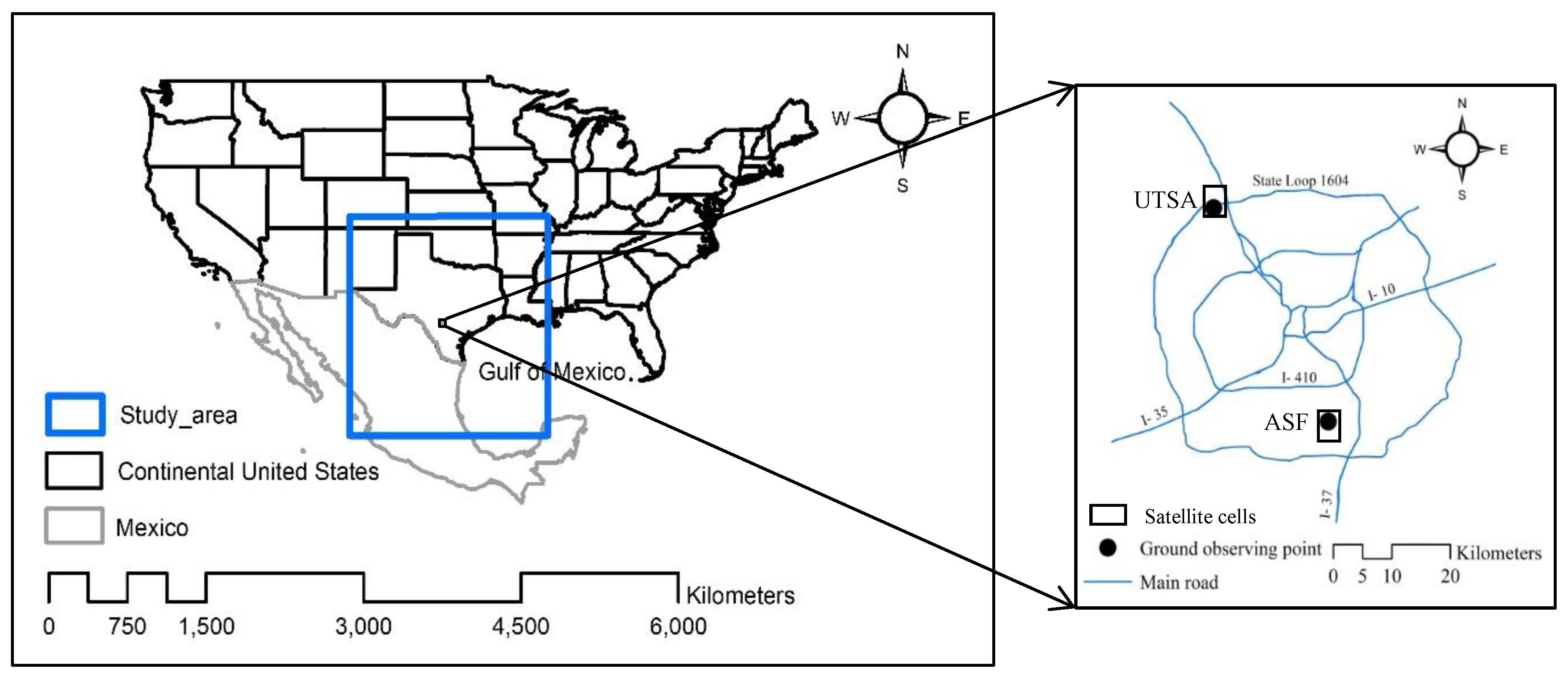
The study area (Figure 1) is a rectangular region of the North American continent (20° N–38° N, 90° W–107° W), which includes, in its northern half, the entire US states of Texas and Oklahoma, as well as fractional areas of other seven US states (Colorado, Kansas, Missouri, New Mexico, Arkansas, Louisiana, and Mississippi). In its southern half, the study region extends into northeast and central Mexico and the western Gulf of Mexico.
The main dataset comes from the Geostationary Operational Environmental Satellite system (GOES), which contributes to sustainable weather monitoring and forecasting operations. The purpose of this satellite observational system is to help researchers better understand land-atmosphere-ocean interactions and how these interactions affect climate. The National Oceanic and Atmospheric Administration (NOAA) currently provides the GOES Surface and Insolation Products (GSIP), which is derived from radiative transfer models [11,12]. The University of Maryland/Shortwave Radiation Budget (UMD/SRB) model, developed by Pinker et al. [13], was applied to GOES satellites for estimating the downward surface solar irradiance, using the irradiance at the top of atmosphere to infer atmospheric transmittance. The GOES data, used in this study, come from GSIP version 2 (GSIP-v2) covering the period from April 1, 2009 to December 31, 2014 with a spatial resolution of 14 km (a total of 41,908 hourly datasets) and GSIP version 3 (GSIP-v3) from March 1, 2014 to October 19, 2016 with a spatial resolution of 4 km (a total of 19,765 hourly datasets). Each GSIP hourly dataset includes daytime spatial fields of cloud types, cloud layers, and global horizontal irradiance in the total solar spectrum band (200–4000 nm) for the study area, based on the visible and infrared channels of GOES East (45 min after the hour) and GOES West (on the hour). The descriptions of the cloud categories used in the analysis are shown in Table 1.
The ground observations of global horizontal irradiance come from two stations, UTSA (University of Texas at San Antonio) (29.5833° N, 98.6199° W) and ASF (Alamo Solar Farm) (29.7010° N, 98.4432° W), which were described in detail in Xia et al. [14]. Briefly, the dataset recorded by a LI-200R pyranometer at the UTSA station covers the periods from May 1 to May 31 and June 24 to October 25, 2015 with a typical uncertainty of 3% and spectral range of 0.4–1.1 µm. The temporal resolution is 5 min. The ASF station provides a dataset recorded by a CMP11_L pyranometer from July 1 to September 31, 2014 and September 22, 2015 to October 18, 2016 with an uncertainty of <2% and spectral range of 0.285–2.8 µm. The time intervals are irregular with a sampling distribution having a mean of 0.16 min and standard deviation of 0.23 min. The number of observations gathered are 18,982 at UTSA and 451,654 at ASF. The cloud and solar irradiance information extracted from the two satellite cells, that include the two ground station locations, is used and comparisons of solar energy potential from satellite and ground observations for the two sites are performed. The GOES satellite-derived solar radiation data was previously validated by Xia et al. [14], who showed that the satellite and ground global horizontal irradiance at the two stations agreed well on hourly and daily timescales under clear and cloudy conditions (correlations ~0.8–0.9).
3. Methods
To characterize the effects of the different cloud categories on solar radiation, the reduced solar irradiance in percentage (ΔSI %) is calculated as follows:
where is the global horizontal irradiance reaching the earth’s surface under clear-sky conditions and is similar to but for all sky conditions. The estimates of in (1) are calculated from the model proposed by Ineichen and Perez [15] and Perez et al. [16]. This equation has been applied in many studies [17,18,19]. It is a model based on Kasten clear sky model [20], which is adjusted for turbidity to improve the fit to observed data.
where is the normal incidence extraterrestrial irradiance; indicates the solar elevation angle; is the altitude corrected air mass [21]; = 5.09 × 10⁻⁵ × altitude + 0.868; = 3.92 × 10⁻⁵ × altitude + 0.0387; = exp(−altitude/8000); = exp(−altitude/1250); and is Linke turbidity available from the Solar Radiation Data website (http://www.soda-pro.com/web-services/atmosphere/linke-turbidity-factor-ozone-water-vapor-and-angstroembeta). A comparison of from Equation (2) against ground observations of clear sky global horizontal irradiance at 30 locations throughout the US by Reno et al. [17] gave a root mean square error of ~5% over many sites.
The solar energy potential (unit: Whm−2) is defined as the total solar energy available to be converted into electric energy (i.e., without taking into account the efficiency of the photovoltaic conversion system) and is calculated by integrating the global horizontal irradiance (unit: Wm−2) over time as follows,
where (unit: h) is the time period of interest (in this study: 1 day, 1 month, 1 season, or 1 year).
4. Results
4.1. Temporal Variability of Cloudiness and Solar Energy Attenuation in San Antonio, Texas
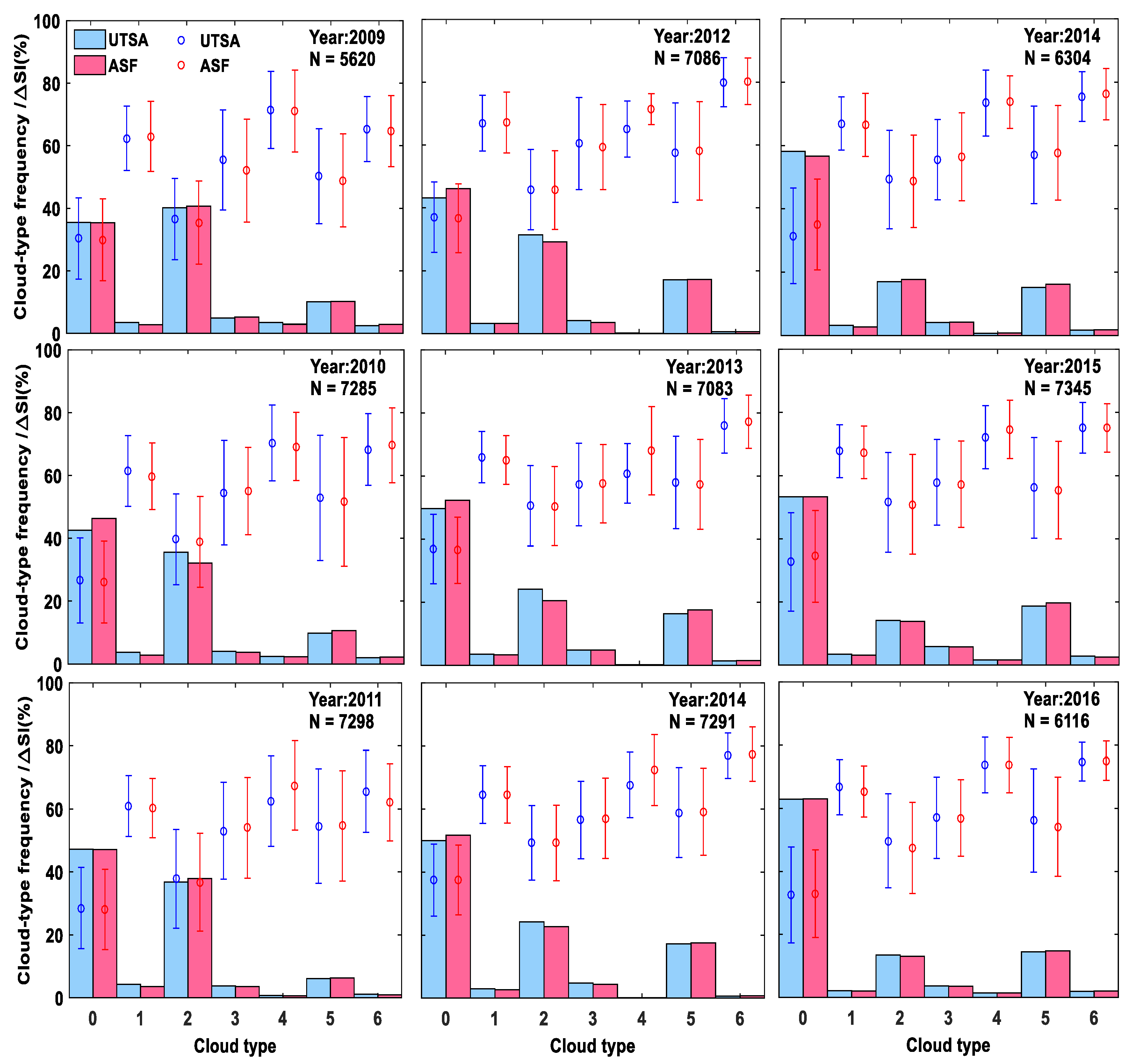
Figure 2 shows the frequency of cloud types and the corresponding reduced solar energy (both in percentage) calculated for each year in 2009–2016 using GSIP-v2 and GSIP-v3 data for the UTSA and ASF locations. The total number of observations for each year (see upper right corner of each panel) is ~7000 except for 2009 and 2016, which are smaller (~6000) as expected, since both are incomplete years missing the first 3, and last ~2 months, respectively.
Figure 3 is similar to Figure 2 but combines all available data for GSIP-v2 and GSIP-v3. When comparing the results for GSIP-v2 and GSIP-v3 in Figure 2 and Figure 3, especially when comparing the overlapping year 2014, it is apparent that GSIP-v2 gives smaller frequency occurrences of clear-sky conditions and greater frequency occurrences of cloudy-sky conditions. It is not clear why this is so, and to the best of our knowledge, there was no previous report that documented these discrepancies. The difference in spatial resolution (14 km for GSIP-v2 versus 4 km for GSIP-v3) could have potentially contributed to such discrepancy. GSIP-v3 has higher spatial resolution and is thus chosen for further analysis of cloud and solar energy potential in this study.
By looking at the 2014, 2015, 2016 plots from GSIP-v3 in Figure 2, it is clear that the frequency of occurrence of cloud types and their attenuation effects are very similar from year to year, i.e., clear-sky conditions are the most common and they cause the least reduction of solar irradiance, and the glaciated clouds and multilayered clouds are always the least common but cause the greater reduction of solar irradiance. The influence of the different cloud types on solar irradiance is found to be the same as expected from [20]. As seen in the GSIP-v3 plot in Figure 3 (right panel), clear skies in both San Antonio locations occur ~57% of the time and reduce solar irradiance by ~33%; cirrus clouds occur ~17% of the time and reduce solar irradiance by ~56%; water clouds occur ~15% of the time and reduce solar irradiance by ~50%; and the other cloud types (mixed, partly, multilayered and glaciated) account for less than 5% of sky conditions and could reduce solar irradiance by 57–75%.
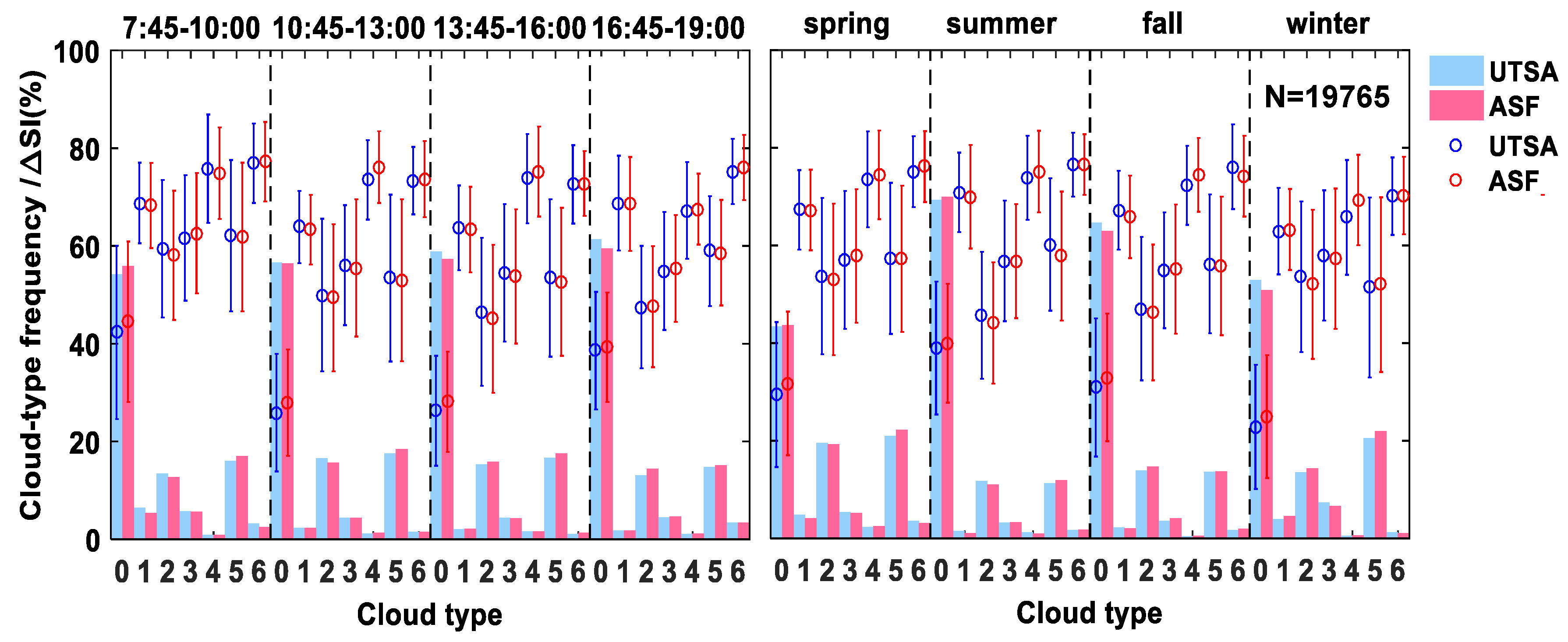
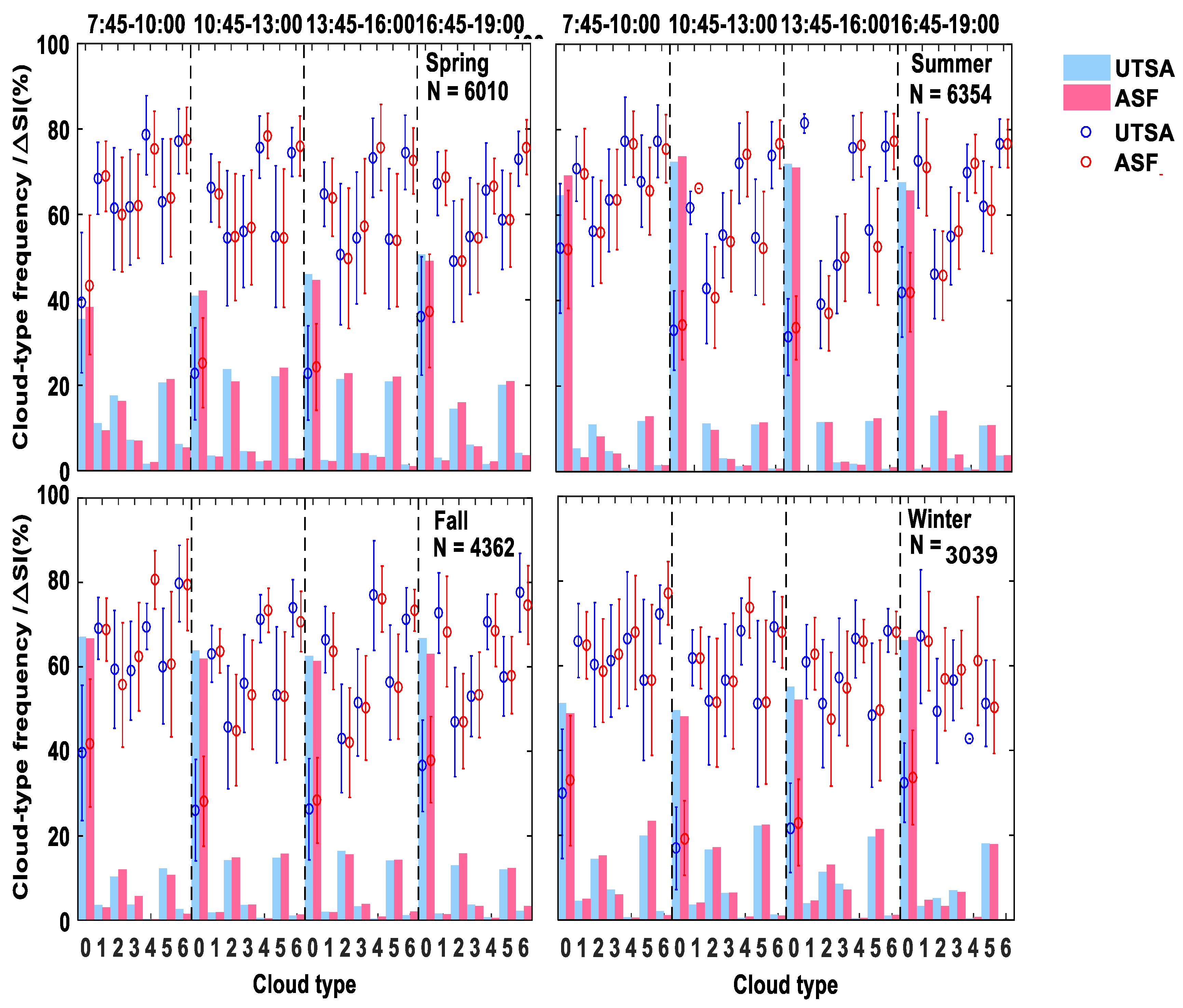
In Figure 4, the diurnal (left panel) and seasonal (right panel) variabilities of cloud properties and their effect on attenuating irradiance are presented. To investigate the daily variations (color bars in Figure 4, left), the frequency of occurrence of cloud types and their respective irradiance attenuation are stratified into four separate even 2.25-h periods: 07:45–10:00 (early morning), 10:45–13:00 (late morning), 13:45–16:00 (early afternoon), and 16:45–19:00 (late afternoon). Overall, the frequency of occurrence of each cloud type does not change much during the day, with the frequency of the clear-sky conditions showing a slight increase from early morning to late afternoon, slightly more noticeable at the UTSA location. The late afternoon (16:45–19:00) has 4–7% more clear-sky conditions than in the early morning (07:45–10:00). Overall, partly and mixed clouds occur more frequently in the early morning than in any other time period. Water, glaciated, and cirrus clouds occur more frequently in the late morning and early afternoon, while the mixed and multi-layered clouds occur more in the early morning and late afternoon.
In terms of the daily variations in solar irradiance attenuation for each cloud type (color error bars in left panel of Figure 4), overall, the attenuation of solar irradiance in percentage is higher in early morning and late afternoon (when the solar zenith angle is larger), with some exceptions. The reduced solar irradiance in percentage under clear-sky conditions is higher with 39–44% in the early morning and late afternoon and lower with 26–28% in the middle of daytime, most likely due to the longer path that solar radiation goes through the atmosphere in the early morning and late afternoon. Under partly, water, mixed, cirrus, and multilayered clouds, the reduced solar irradiance in percentage is the highest in the early morning and the lowest in the early afternoon. The reduced solar irradiance under glaciated clouds is the lowest with ~67% in the late afternoon than any other time periods.
To investigate the seasonal variations (Figure 4, right), the frequency of occurrence of cloud types and their respective irradiance attenuation are stratified into four separate three-month periods: Winter (December-February), spring (March–May), summer (June-August), and fall (September-November). The frequencies of clear-sky occurrences are the highest in summer (69%) and the lowest in spring (43%). Water and cirrus clouds are the most common in spring (19–22%) and the least common in summer (11–12%). Partly and mixed clouds are more common in spring and winter but less common in summer and fall. Glaciated and multi-layered clouds are more common in spring than in any other seasons. Overall, the attenuation of solar irradiance for each cloud type varies only slightly from season to season.
To investigate the daily variations in each season, Figure 5 shows the frequency of occurrence and irradiance attenuation for each cloud type stratified as in Figure 4 (left) but for each season defined as in Figure 4 (right). The frequencies of occurrence of cloud types are different for each season. The frequency of occurrence of clear-sky conditions in spring is similar to the all-season average shown in Figure 4 (left), although the frequency of occurrence in spring is much smaller than the all-season averaged and also smaller compared with to the other three seasons. Summer has the highest clear-sky percentage of occurrence with even higher values in the late morning and early afternoon than in the two other time periods. Fall has the second highest clear-sky percentage, with the highest frequency in the early morning period. Winter ranks the fourth in terms of clear-sky frequency of occurrence, with the highest frequency in the late afternoon period. Note that the patterns of reduced solar irradiance in percentage by cloud types during each time period, among four seasons, are similar, but with slightly different magnitudes.
4.2. Spatial Distribution of Clouds and Solar Energy Potential in Texas and Nearby Regions
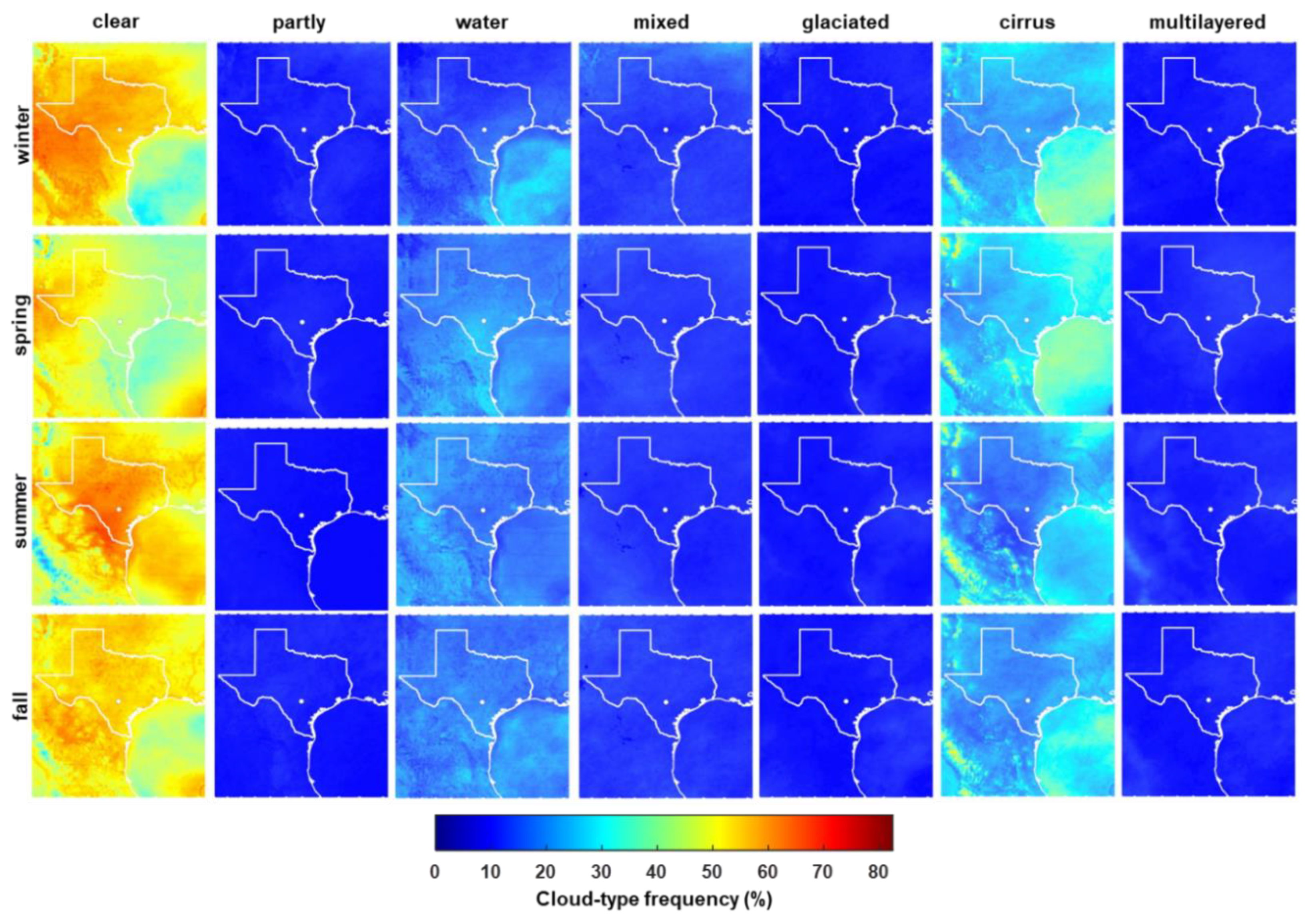
Figure 6 and Figure 7 show the seasonal distribution of cloud-type and cloud-layer frequencies for the four seasons over the study area. In Figure 6, clear-sky conditions overall are more common than cloudy-sky conditions. Cirrus is the most common cloud type, followed by water clouds. The other four types (partly, mixed, glaciated, and multilayered) are less common (mostly less than 15%). All of these results are consistent with the findings for the two San Antonio locations presented in Section 4.1. The frequency of clear sky conditions in winter is higher in the center and western parts of the study area, especially in the northern Mexico region; in spring, it is higher mostly in the western-most (middle latitudes) region of the study area and in the southeastern corner over the Gulf of Mexico; in summer, it is higher mainly in Texas and northeast region of Mexico, with higher frequencies also over the Gulf of Mexico; in fall, the frequency of clear sky is more homogeneous in space, except for some lower frequency spots in the Gulf of Mexico and near the Sierra Madre Occidental in Mexico. The Sierra Madre Occidental also has low frequency of clear sky in summer, perhaps due to topographic blocking of clouds and/or clouds formed over the range with warm moist air rising up.
The frequency of cirrus clouds is relatively higher in Gulf of Mexico and lower over land areas, except along the Sierra Madre Occidental where the cirrus clouds seem occur frequently in all seasons which is consistent with the lower frequency of clear-sky conditions in these region noted earlier for the summer but that it is apparent also in the other seasons in Figure 6. Water clouds have higher frequencies in the Gulf of Mexico in winter, while this seems to occur more frequently over land than over the ocean in spring and summer, with a more homogeneous spatial distribution in the fall.
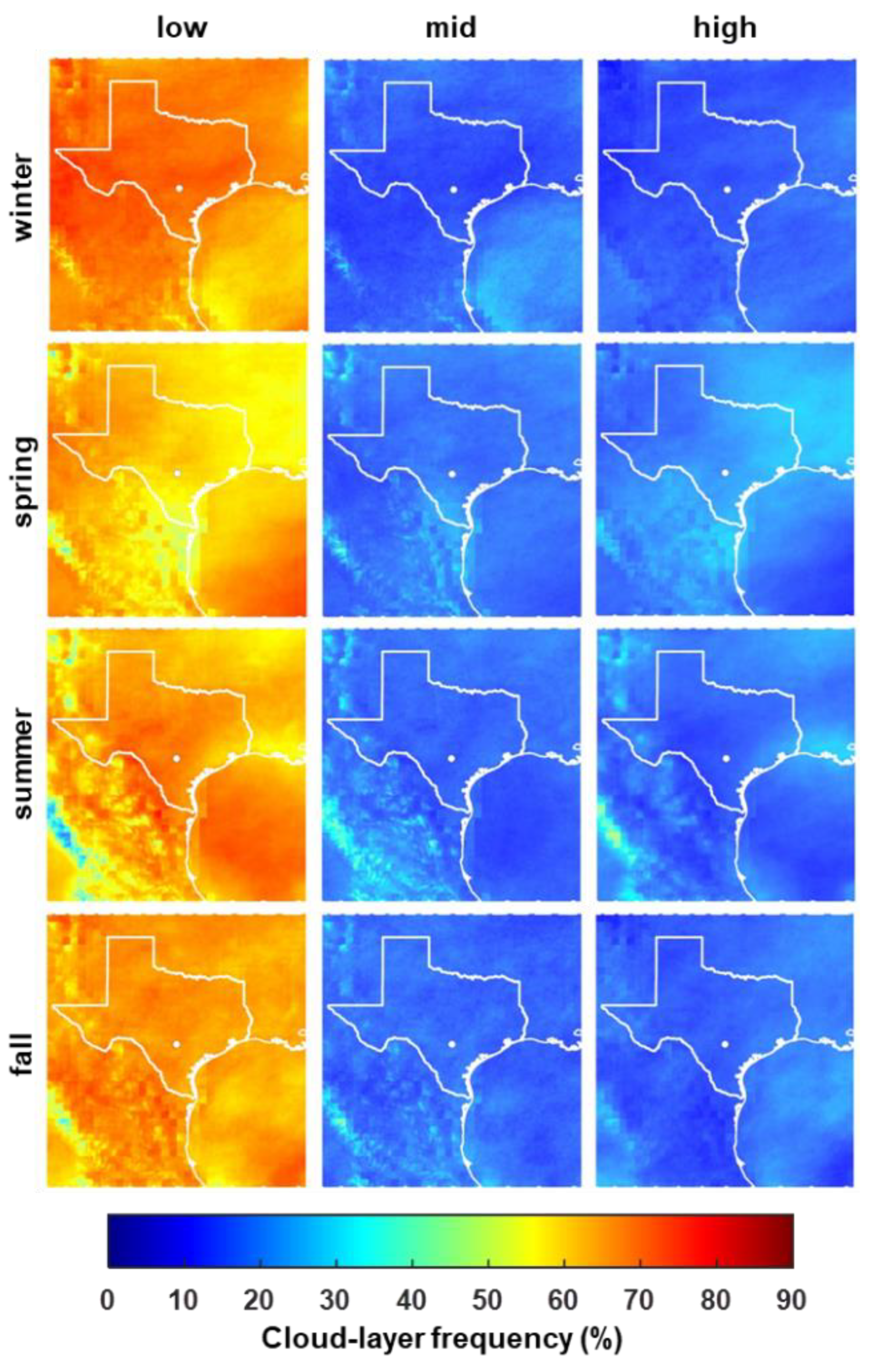
In terms of the overall spatial distribution of cloud-layer frequencies (Figure 7), low clouds occur more frequently. Around Texas, the frequencies of low clouds are higher in winter and lower in spring. In the Gulf of Mexico, low clouds are more frequent in summer and less frequent in winter. Mid altitude clouds occur more frequently in winter/fall than in the other seasons over the Gulf of Mexico. Over land, high clouds occur more frequently in spring and over the ocean in spring/fall. The Sierra Madre Occidental shows higher frequency of mid- and high-clouds, but less frequency of low clouds than other areas.
The monthly spatial distribution of solar energy potential is presented in Figure 8. Depending on the calendar month and location, the monthly solar energy potential ranges from 43–254 kWhm−2. from November to January, the solar energy in the north to northeast part of the study area is quite low (<100 kWhm−2). It is higher in parts of Mexico and the Gulf of Mexico, but less than 160 kWhm−2. In February, the solar energy potential increases, especially over Mexico and the Gulf of Mexico, with the increases of 10-30 kWhm−2 in the central region of the study area. In March, the solar energy in the southwestern and southeastern corners of the study area reach values of 190–210 kWhm−2. In this month, the northwestern Texas region has a monthly solar energy potential of 150–180 kWhm−2 and the northeastern Texas region still has low values. From April to July, the available solar energy continues to increase to reach maximum values over most of the study area. An exception is the Sierra Madre Occidental, where the energy potential reaches maximum values in May. In August, the solar energy potential over most of the study area starts to drop to 180–210 kWhm−2 over Texas. The available solar energy over Gulf of Mexico drops by 10–20%, but is still higher than that any region over land. In September, the distribution of solar energy seems relatively homogeneous, with overall values of 140–200 kWhm-2. The Gulf of Mexico receives significantly less solar energy in September than in any month in the period March-August. In October, the solar energy potential in the upper part of the study area generally drops to 100–150 kWhm−2, while it ranges from 150–180 kWhm−2 over Gulf of Mexico.
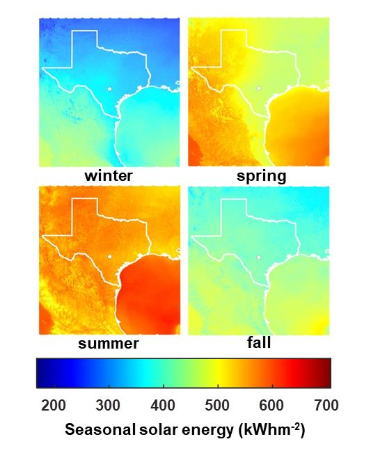
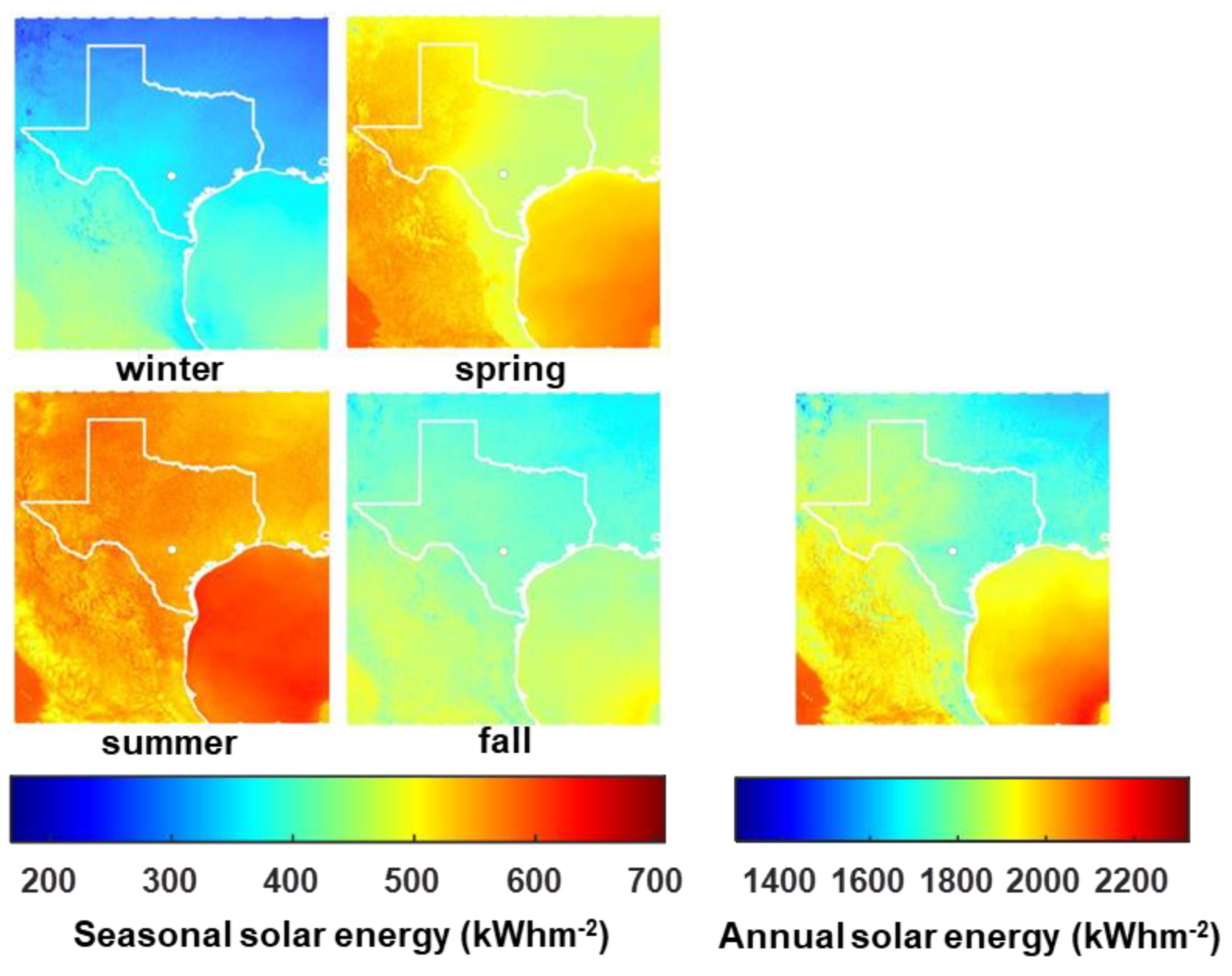
The available seasonal solar energy potential ranges from 165-710 kWhm−2 (Figure 9) with maximum vales in summer and minimum in winter. In winter, the seasonal solar energy potential does not exceed 350 kWhm−2 over the most of Texas and 420 kWhm−2 over Gulf of Mexico. In spring, the seasonal energy potential increases to more than 500 kWhm−2 over Texas with parts of Mexico and the Gulf of Mexico receiving more than 600 kWhm−2. The highest amount of solar energy is received in summer over the entire study area, particularly in the Gulf of Mexico. In fall, the seasonal energy potential drops by 300–450 kWhm−2 over the entire study area.
The annual solar energy, shown in the bottom right panel of Figure 9, is derived only for the year 2015, because it is the only complete year in the GSIP-v3 dataset. The annual energy potential ranges from 1300–2300 kWhm−2. The northeastern region of the study area receives lower values of solar energy (less than 1800 kWhm−2). The north-western part of Texas receives 50–200 kWhm−2 more energy than the rest of Texas. The Gulf of Mexico and Mexico receive more solar energy than Texas and the north-eastern region of the study area.
4.3. Time Series of Solar Energy Potential in San Antonio, Texas
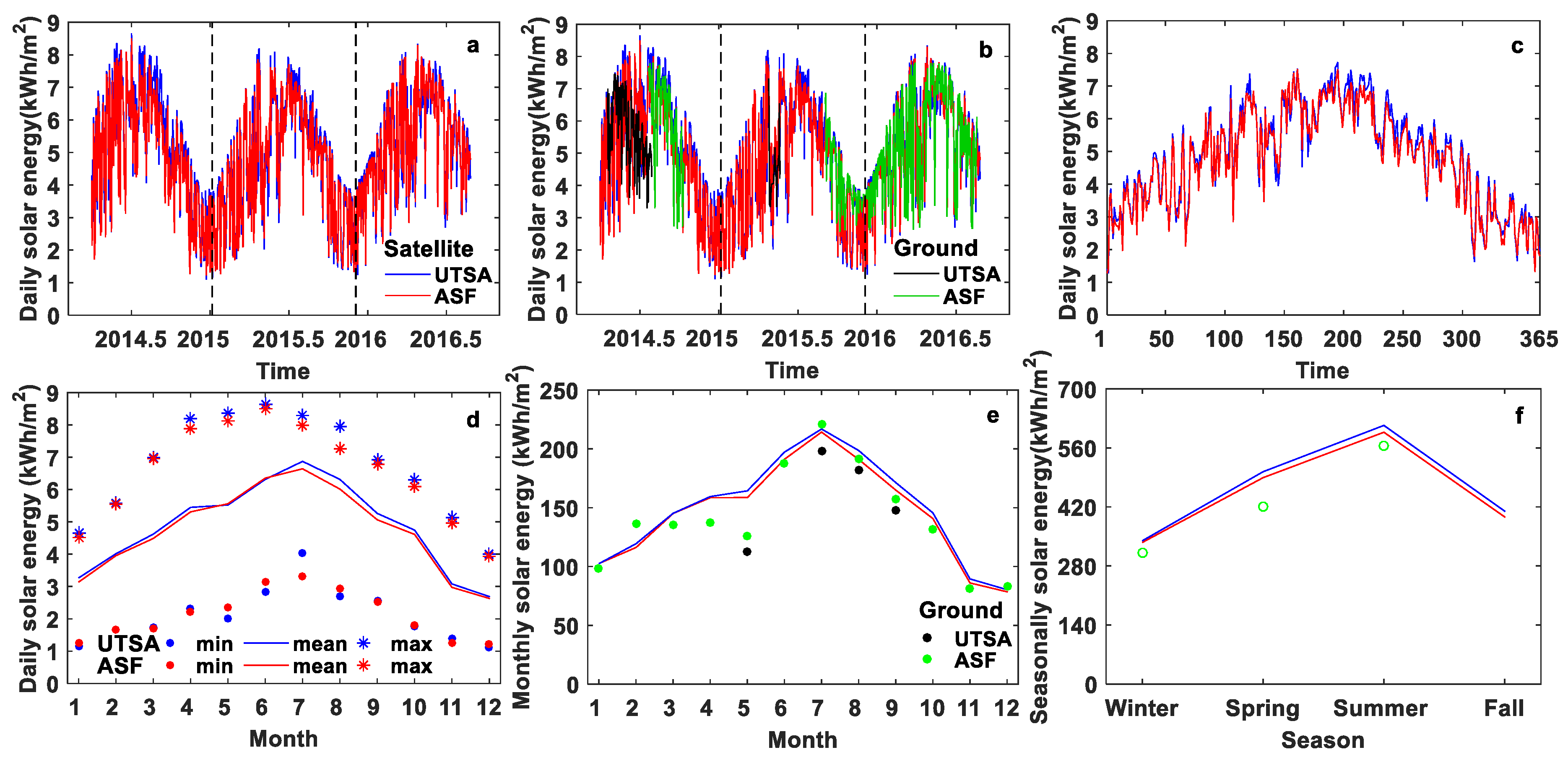
As an example of the daily, monthly, and seasonal solar energy potential time series derived from the satellite data, the time series at UTSA and ASF are presented in Figure 10. For both UTSA and ASF, it is found that the highest daily solar energy potential is ~8.58 kWhm−2 on June 10, 2014 but the lowest is 1.16 kWhm−2 on December 17, 2014. The min, mean, and max values of daily solar energy in each month are also presented. The monthly solar energy varies from 79 to 217 kWhm−2. from October to February, the monthly solar energy does not exceed 120 kWhm−2, while it is consistently above 145 kWh m−2 from March to September. The range of monthly solar energy potential reaches 155–200 kWh m−2 in April, May and June. In July, the range of solar energy potential is close to 210–225 kWh m−2. The solar energy potential drops to 190–200 kWhm−2 in September. The seasonal solar energy potential reaches the highest values 595–615 kWhm−2 in summer and the lowest values 335–340 kWhm−2 in winter. In fall, it reaches values of 395–410 kWhm−2. The received solar energy in spring is around 485–510 kWhm−2. The annual solar energy potential is 1750 kWhm−2. A general good agreement is found between satellite-derived solar energy potential and the estimated energy potential from ground observations at the UTSA and ASF stations, as expected from Xia et al. [14] who found that the global horizontal irradiances from satellite and ground at the two stations also agreed well (correlations 0.80–0.87 on the hourly timescale and 0.94–0.91 on the daily timescale). In most cases, the satellite-derived monthly solar energy potential is higher than that derived from the ground observations, except in February and July. The highest difference in monthly solar energy potential is observed in May, followed by September. For the seasonal energy potential the larger difference between satellite and ground estimates is found in spring.
5. Discussion
Satellite data is used to retrieve information on clouds, cloud effects on solar irradiance, and to derive the available monthly, seasonal, and annual solar energy potential in San Antonio, Texas and surrounding regions during 2014–2016. The clouds are critical in determining how much solar radiation reaches the surface of the earth. Their effects on solar radiation is dependent on thickness, horizontal extent, horizontal variability, water content, phase (liquid or ice), the size of the droplets and crystal and height of clouds. It is essential to distinguish different cloud types for calculating the reduced solar irradiance in percentage. The regional and seasonal characteristics of clouds are analyzed with solar energy derived from satellites and compared to ground estimates.
It is found that clear-sky conditions occur more frequently than any other cloud-condition over the study area. The spatial distribution of clouds shows regional differences in the frequency of cloud-type and cloud-layer occurrence. The frequency of the clear-sky conditions is much higher over the land as compared with that over the ocean in the study area. This is because the warm moist air over the ocean rises, cools down by the adiabatic effect of lesser pressure aloft, and then condenses into clouds. It is interesting that there is an increasing frequency of the cloud-sky conditions observed during the summer season in Sierra Madre Occidental, which is a major mountain range system of the North American Cordillera that runs northwest–southeast through Northwestern and Western Mexico, and along the Gulf of California. The mountain is warmer than the surrounding air, causing the air to rise to form clouds. The ocean is significantly cloudier than the land, particularly in regards to low clouds, which is expected as reported previously by others [22,23]. The most frequent occurrence of clouds is cirrus, since the tropical deep convective regions, particularly over the Gulf of Mexico in our study area, is generally capped by cirrus clouds [24,25].
The solar energy potential over Gulf of Mexico is significantly higher than that over land, although it has higher frequency of clouds. This is because most clouds over the ocean are cirrus clouds that have relatively less reduction of solar irradiance (Figure 6). Other clouds, partly and mixed phase clouds, are less frequent over Gulf of Mexico than over the land. Further, the seasonal variation of clouds depicts that clouds are less frequent in summer than that in winter. Cloud development is mostly dependent on temperature and the amount of water vapor in the air. The temperature has to be low enough for water vapor to condense into water droplets. During the winter, the temperature of the air in the lower part of the atmosphere is lower than during summer, therefore clouds can usually form at lower height. Since the overall temperature is warmer in summer, it is harder for water vapor to condense into clouds. The reduced solar energy in percentage under different clouds slightly varies from season to season. More cloud types occur in the early morning and late afternoon (high zenith angles) in spring and summer, compared to the fall and winter seasons, and solar beams travel a longer path through the atmosphere and might interact with clouds along the path at high zenith angles, resulting in more attenuation of solar radiation.
It is clear that the solar irradiance in the summer is significantly higher than in the winter. In our study area of Texas and its surrounding regions, the solar energy potential is higher in summer than that in winter. Compared to other regions, the solar energy potential over Texas is significant higher than that over Hong Kong and over the mountain area of Pindos in Greece [7,10,26], mainly due to lesser clouds in Texas and its surrounding areas.
6. Conclusions
Hourly satellite observations of surface solar irradiance and cloud properties (cloud types and layers) from GSIP-v3 with a spatial resolution of 4 km are used to assess the impact of clouds on solar energy potential in San Antonio, Texas, USA and surrounding areas which include northern Mexico and the western Gulf of Mexico. A total of 19,765 hourly satellite datasets of global horizontal irradiance and cloud properties at two locations namely UTSA (29.5833° N, 98.6199° W) and ASF (29.7010° N, 98.4432° W) were used. These are the locations of the two ground stations that were used to validate the satellite estimates of global horizontal irradiance with direct measurements in our previous work. The time periods of ground global horizontal irradiance observations used are 1 May 2015–31 May 2015 and 24 June 2015–25 October 2015 for UTSA and 1 July 2014–31 September 2014 and 22 September 2015–18 October 2016 for ASF. The satellite-derived cloud data at these two station locations reveal that the frequency of occurrence of the various cloud conditions from highest to lowest is: clear sky (~57%), cirrus (~17%), water (~15%), mixed (4%), partly (3%), multilayered (2%), and glaciated (1%). The order of the reduced solar irradiance in percentage from highest to lowest is multilayered (75%), glaciated (73%), partly (66%), mixed and cirrus (57%), water (50%), and clear (33%). When the daytime hours are taken into consideration by sorting the data into four equal time periods, the reduced solar energy in percentage under each cloud type is found to be larger in early morning and late afternoon. This is likely due to the longer path that solar radiation travels through the atmosphere, during these times. When the seasons are taken into account, the frequencies of clear-sky conditions show maximum values in the summer, and minimum in spring, while the frequencies of water and cirrus clouds show opposite behavior. Partly- and mixed-clouds are more common in spring and winter, but less so in summer and fall. Glaciated and multi-layered clouds are more common in spring than in any other season.
The results obtained for available daily, monthly, seasonal, and annual solar energy with a spatial resolution of 4 km are promising for San Antonio, Texas, USA and surrounding areas, which include northern Mexico and the western Gulf of Mexico. The monthly solar energy potential in the study area ranges from 43–254 kWhm−2, with a maximum in July and a minimum in December. The seasonal solar energy potential ranges from 165–710 kWhm−2 with the highest in summer and the lowest in winter. The annual solar energy potential for 2015 varies in space from 1300 to 2300 kWhm−2 with the highest value observed in the Gulf of Mexico and Mexico, followed by the northwest part of Texas, with the lowest value in the northeast part of the study area. The satellite-based solar energy potential for the UTSA and ASF cells are compared with the corresponding ground measurements at the two stations and, as expected, an overall good agreement is found. The findings from this study could inform the policy-decision process on the use of potential renewable energy for any sub region in the study area. It could also enable detailed spatial estimations of city-wide solar energy potential, a necessary first step in determining how much solar energy could be harnessed as electricity and fed into the electrical grid. The ability to accurately forecast cloud and solar irradiance will help electricity grid operators to better schedule, dispatch, and regulate power. Future work will focus on short-term cloud and solar irradiance forecast in the San Antonio area for the efficient operation of solar power plants.
Author Contributions
All authors contributed to the conceptualization; S.X. performed the formal analysis and original draft writing; A.M.M.-N. and H.X. contributed to the supervision; all authors contributed to the review and editing.
Funding
This research received no external funding.
Acknowledgments
This work is supported by CPS Energy and Texas Sustainable Energy Research Institute (TSERI) at the University of Texas at San Antonio (UTSA) and the Department of Geological Sciences at UTSA.
Conflicts of Interest
The authors declare no conflict of interest.
References
- Chow, C.W.; Urquhart, B.; Lave, M.; Dominguez, A.; Kleissl, J.; Shields, J.; Washom, B. Intra-hour forecasting with a total sky imager at the UC San Diego solar energy testbed. Sol. Energy 2011, 85, 2881–2893. [Google Scholar] [CrossRef]
- Stoffel, T. US Department of Energy Workshop Report: Solar Resources and Forecasting. Contract 2012, 303, 275–3000. [Google Scholar]
- Kleissl, J. Solar Energy Forecasting and Resource Assessment; Academic Press: San Diego, CA, USA, 2013. [Google Scholar]
- Voskrebenzev, A.; Riechelmann, S.; Bais, A.; Slaper, H.; Seckmeyer, G. Estimating probability distributions of solar irradiance. Theoret. Appl. Climatol. 2015, 119, 465–479. [Google Scholar] [CrossRef]
- Pfister, G.; McKenzie, R.L.; Liley, J.B.; Thomas, A.; Forgan, B.W.; Long, C.N. Cloud coverage based on all-sky imaging and its impact on surface solar irradiance. J. Appl. Meteor. 2003, 42, 1421–1434. [Google Scholar] [CrossRef]
- Mubiru, J.; Banda, E.J.K.B.; D’Ujanga, F.; Senyonga, T. Assessing the distribution of monthly mean hourly solar irradiation at an African Equatorial site. Energy Convers. Mgmt. 2007, 48, 380–383. [Google Scholar] [CrossRef]
- Nikitidou, E.; Kazantzidis, A.; Tzoumanikas, P.; Salamalikis, V.; Bais, A.F. Retrieval of surface solar irradiance, based on satellite-derived cloud information, in Greece. Energy 2015, 90, 776–783. [Google Scholar] [CrossRef]
- Amillo, A.G.; Ntsangwane, L.; Huld, T.; Trentmann, J. Comparison of satellite-retrieved high-resolution solar radiation datasets for South Africa. J. Energy S. Afr. 2018, 29, 63–76. [Google Scholar] [CrossRef]
- Frank, C.W.; Wahl, S.; Keller, J.D.; Pospichal, B.; Hense, A.; Crewell, S. Bias correction of a novel European reanalysis data set for solar energy applications. Sol. Energy 2018, 164, 12–24. [Google Scholar] [CrossRef]
- Wong, M.S.; Zhu, R.; Liu, Z.; Lu, L.; Peng, J.; Tang, Z.; Lo, C.H.; Chan, W.K. Estimation of Hong Kong’s solar energy potential using GIS and remote sensing technologies. Renew. Energy 2016, 99, 325–335. [Google Scholar] [CrossRef]
- Pinker, R.T.; Laszlo, I. Modeling surface solar irradiance for satellite applications on a global scale. J. Appl. Meteor. 1992, 31, 194–211. [Google Scholar] [CrossRef]
- Pinker, R.T.; Frouin, R.; Li, Z. A review of satellite methods to derive surface shortwave irradiance. Remote Sens. Environ. 1995, 51, 108–124. [Google Scholar] [CrossRef]
- Pinker, R.T.; Tarpley, J.D.; Laszlo, I.; Mitchell, K.E.; Houser, P.R.; Wood, E.F.; Schaake, J.C.; Robock, A.; Lohmann, D.; Cosgrove, B.A.; et al. Surface radiation budgets in support of the GEWEX Continental-Scale International Project (GCIP) and the GEWEX Americas Prediction Project (GAPP), including the North American Land Data Assimilation System (NLDAS) project: GEWEX Continental-Scale International Project, Part 3 (GCIP3). J. Geophys. Res. 2003, 108. [Google Scholar]
- Xia, S.; Mestas-Nuñez, A.M.; Xie, H.; Vega, R. An Evaluation of Satellite Estimates of Solar Surface Irradiance Using Ground Observations in San Antonio, Texas, USA. Remote Sens. 2017, 9, 1268. [Google Scholar] [CrossRef]
- Ineichen, P.; Perez, R. A new airmass independent formulation for the Linke turbidity coefficient. Sol. Energy 2002, 73, 151–157. [Google Scholar] [CrossRef] [Green Version]
- Perez, R.; Ineichen, P.; Moore, K.; Kmiecik, M.; Chain, C.; George, R.; Vignola, F. A new operational model for satellite-derived irradiances: description and validation. Sol. Energy 2002, 73, 307–317. [Google Scholar] [CrossRef] [Green Version]
- Reno, M.J.; Hansen, C.W.; Stein, J.S. Global Horizontal Irradiance Clear Sky Models: Implementation and Analysis. SANDIA report SAND2012-2389. 2012. Available online: http://citeseerx.ist.psu.edu/viewdoc/download?doi=10.1.1.651.1676&rep=rep1&type=pdf (accessed on 10 May 2019).
- Schillings, C.; Meyer, R.; Trieb, F. Solar and Wind Energy Resource Assessment (SWERA). DLR—activities within SWERA. Available online: https://openei.org/datasets/files/712/pub/sri_lanka_10km_solar_country_report.pdf (accessed on 10 May 2019).
- Jia, Y. Solar Shift: A perspective on Building Energy Performance under Haze Pollutions in China; Georgia Institute of Technology: Atlanta, GA, USA, 2016. [Google Scholar]
- Xia, S.; Mestas-Nuñez, A.; Xie, H.; Tang, J.; Vega, R. Characterizing Variability of Solar Irradiance in San Antonio, Texas Using Satellite Observations of Cloudiness. Remote Sens. 2018, 10, 2016. [Google Scholar] [CrossRef]
- Kasten, F.; Young, A.T. Revised optical air mass tables and approximation formula. Appl. Optics. 1989, 28, 4735–4738. [Google Scholar] [CrossRef] [PubMed]
- Hahn, C.J.; Warren, S.G. A Gridded Climatology of Clouds over Land (1971-96) And Ocean (1954-97) from Surface Observations Worldwide; Report ORNL/CDIAC-153 NDP-026-E; US Department of Energy: Oak Ridge, TN, USA, 2007.
- Eastman, R.; Warren, S.G.; Hahn, C.J. Variations in cloud cover and cloud types over the ocean from surface observations, 1954–2008. J. Climate. 2011, 24, 5914–5934. [Google Scholar] [CrossRef]
- Sassen, K.; Wang, Z.; Liu, D. Cirrus clouds and deep convection in the tropics: Insights from CALIPSO and CloudSat. J. Geophys. Res. 2009, 114, D00H06. [Google Scholar] [CrossRef]
- Gupta, A.K.; Rajeev, K.; Sijikumar, S.; Nair, A.K.M. Enhanced daytime occurrence of clouds in the tropical upper troposphere over land and ocean. Atmos. Res. 2018, 201, 133–143. [Google Scholar] [CrossRef]
- Kosmopoulos, P.G.; Kazadzis, S.; Taylor, M.; Bais, A.F.; Lagouvardos, K.; Kotroni, V.; Keramitsoglou, I.; Kiranoudis, C. Estimation of the solar energy potential in Greece using satellite and ground-based observations. In Perspectives on Atmospheric Sciences; Springer: Athens, Greece, 2017; pp. 1149–1156. [Google Scholar]
Figure 1.
The left panel shows the state boundaries of the contiguous United States to the north and of Mexico to the south with the location of the study area (i.e., Texas and surrounding regions) superimposed as a blue box. The city of San Antonio, Texas is indicated as a small open square near the center of the study region. The right panel is an expanded view of San Antonio showing the locations of the two ground stations (black dots) and their overlapping satellite cells (black boxes) relative to the city’s main highways (blue lines).

Figure 2.
Percentage plots of cloud-type frequency (color bars) and reduced solar irradiance (color error bars of mean ± 1 standard deviation) versus the seven cloud types of Table 1 using GSIP-v2 (left two columns) and GSIP-v3 (right column) datasets for each year in 2009–2016 and for the two station locations (University of Texas at San Antonio (UTSA): Light blue color bars and blue error bars; Alamo Solar Farm (ASF): Pink color bars and red error bars). The year and the number of samples used for each plot (N) are given in the upper right corner of each panel. Note that there are two panels for 2014 because on that year the GSIP-v2 and GSIP-v3 datasets overlap each other.

Figure 3.
Similar to Figure 2, but combining all available data for GSIP-v2 (left panel) and GSIP-v3 (right panel).
Figure 3.
Similar to Figure 2, but combining all available data for GSIP-v2 (left panel) and GSIP-v3 (right panel).

Figure 4.
Similar to Figure 2, but using only the GSIP-v3 dataset at the two station locations for four 2.25 h time periods (07:45–10:00, 10:45–13:00, 13:45–16:00, and 16:45–19:00) (left panel) and for the four seasons as defined in the text (right panel).
Figure 4.
Similar to Figure 2, but using only the GSIP-v3 dataset at the two station locations for four 2.25 h time periods (07:45–10:00, 10:45–13:00, 13:45–16:00, and 16:45–19:00) (left panel) and for the four seasons as defined in the text (right panel).

Figure 5.
Same as the left panel in Figure 4, but for each of the four seasons as defined in the text.
Figure 5.
Same as the left panel in Figure 4, but for each of the four seasons as defined in the text.

Figure 6.
The seasonal cloud-type frequency derived from GSIP-v3 data of 2014-2016.

Figure 7.
Same as Figure 6, but for cloud layers.
Figure 7.
Same as Figure 6, but for cloud layers.

Figure 8.
The monthly solar energy potential derived from GSIP-v3 over the study area.

Figure 9.
The seasonal (2014-2016) and annual (2015) solar energy potential derived from GSIP-v3.

Figure 10.
The daily, monthly and seasonal accumulative solar energy derived from GSIP-v3 for the two cells where two stations (UTSA and ASF) are located: (a) The daily solar energy derived from satellite GSIP-v3 for the two stations; (b) the daily solar energy of station measurements overlaid on that derived from satellites; (c) the average daily solar energy derived from satellite GSIP-v3 for 365 days; (d) the min, mean, and max daily solar energy derived from satellite GSIP-v3 in each month; (e) monthly solar energy derived from satellite GSIP-v3 and the ground; and (f) the seasonal solar energy derived from satellite GSIP-v3 and the ground (noting UTSA site does not contain enough ground data to make seasonal numbers).


Table 1.
Geostationary Operational Environmental Satellite (GOES) Surface and Insolation Products (GSIP) cloud categories adapted from [14].
Table 1.
Geostationary Operational Environmental Satellite (GOES) Surface and Insolation Products (GSIP) cloud categories adapted from [14].
| Cloud Category | Classification ID | Description |
|---|---|---|
| Cloud type | 0 | clear |
| 1 | partly (partly cloudy/fog) | |
| 2 | water (water cloud) | |
| 3 | mixed (supercooled/mixed-phase cloud) | |
| 4 | glaciated (optically thick ice cloud) | |
| 5 | cirrus (optically thin ice cloud) | |
| 6 | multilayered (cirrus over lower cloud) | |
| Cloud layer | 1 | low (0–2 km) |
| 2 | mid (2–7 km) | |
| 3 | high (5–13 km) |
© 2019 by the authors. Licensee MDPI, Basel, Switzerland. This article is an open access article distributed under the terms and conditions of the Creative Commons Attribution (CC BY) license (http://creativecommons.org/licenses/by/4.0/).
Share and Cite
MDPI and ACS Style
Xia, S.; Mestas-Nuñez, A.M.; Xie, H.; Vega, R. Satellite-based Cloudiness and Solar Energy Potential in Texas and Surrounding Regions. Remote Sens. 2019, 11, 1130. https://0-doi-org.brum.beds.ac.uk/10.3390/rs11091130
AMA Style
Xia S, Mestas-Nuñez AM, Xie H, Vega R. Satellite-based Cloudiness and Solar Energy Potential in Texas and Surrounding Regions. Remote Sensing. 2019; 11(9):1130. https://0-doi-org.brum.beds.ac.uk/10.3390/rs11091130
Chicago/Turabian StyleXia, Shuang, Alberto M. Mestas-Nuñez, Hongjie Xie, and Rolando Vega. 2019. "Satellite-based Cloudiness and Solar Energy Potential in Texas and Surrounding Regions" Remote Sensing 11, no. 9: 1130. https://0-doi-org.brum.beds.ac.uk/10.3390/rs11091130
Note that from the first issue of 2016, this journal uses article numbers instead of page numbers. See further details here.