Cohesion Intensive Deep Hashing for Remote Sensing Image Retrieval


1
College of Oceanography and Space Informatics, China University of Petroleum (East China), 66 Changjiang West Road, Qingdao 266580, China
2
School of Computer Science and Engineering, Beihang University, Beijing 100191, China
3
School of Computing, National College of Ireland, 1 D01 K6W2 Dublin, Ireland
4
Institute of Information Engineering, Chinese Academy of Sciences, Beijing 100093, China
*
Author to whom correspondence should be addressed.
Remote Sens. 2020, 12(1), 101; https://0-doi-org.brum.beds.ac.uk/10.3390/rs12010101
Submission received: 28 October 2019
/
Revised: 22 December 2019
/
Accepted: 25 December 2019
/
Published: 27 December 2019
(This article belongs to the Section Remote Sensing Image Processing)
Abstract
:Recently, the demand for remote sensing image retrieval is growing and attracting the interest of many researchers because of the increasing number of remote sensing images. Hashing, as a method of retrieving images, has been widely applied to remote sensing image retrieval. In order to improve hashing performance, we develop a cohesion intensive deep hashing model for remote sensing image retrieval. The underlying architecture of our deep model is motivated by the state-of-the-art residual net. Residual nets aim at avoiding gradient vanishing and gradient explosion when the net reaches a certain depth. However, different from the residual net which outputs multiple class-labels, we present a residual hash net that is terminated by a Heaviside-like function for binarizing remote sensing images. In this scenario, the representational power of the residual net architecture is exploited to establish an end-to-end deep hashing model. The residual hash net is trained subject to a weighted loss strategy that intensifies the cohesiveness of image hash codes within one class. This effectively addresses the data imbalance problem normally arising in remote sensing image retrieval tasks. Furthermore, we adopted a gradualness optimization method for obtaining optimal model parameters in order to favor accurate binary codes with little quantization error. We conduct comparative experiments on large-scale remote sensing data sets such as UCMerced and AID. The experimental results validate the hypothesis that our method improves the performance of current remote sensing image retrieval.

1. Introduction
1.1. Background
The data set volume of remote sensing images has been expanding rapidly [1,2,3]. Remote sensing images have a wide range of applications including remote sensing scene classification [4] and scene-driven object detection [5]. It is difficult to efficiently find one image with specific content in an extremely large data set. Therefore, effective retrieval based on content has become one important problem in the literature of remote sensing. Content-based image retrieval (CBIR) extracts the content information of images and retrieves them by matching the content information between images. CBIR reduces the process of manual annotation and improves the retrieval efficiency. It has been widely applied in disaster prevention, soil erosion monitoring [6], etc.
As one class of CBIR, hashing is a family of quantization techniques and enables efficient and effective retrieval of target remote sensing images [7]. It quantizes remote sensing images into fixed-length binary codes, which are referred to as hash codes. In hash-code-based retrieval operations, the hash codes are used for efficiently measuring the distance between images, and the images having small distance with the inquiry image are returned as retrieval results. Benefiting from the binary representations, hashing-based image retrieval renders a fast retrieval speed with simple operations. Conventional hashing methods such as locality sensitive hashing (LSH) [8], spectral hashing (SH) [9], and iterative quantization (ITQ) [10] have been applied to various tasks including image retrieval. Luka et al. [11] were among the first to introduce hashing into remote sensing image retrieval by proposing an improved LSH-based image hashing method. Demir et al. [12] developed a kernelized locality sensitive hashing (KLSH) and a supervised hashing model with kernels (KSH) for retrieving remote sensing images. Li et al. [13] proposed an unsupervised partial randomness hashing (PRH) method. Li et al. [14] developed an online hash algorithm which is capable of processing continuously updated image data.
Most of the conventional hashing methods rely on the hand-crafted image features. The hand-craft image features refer to those extracted by hand-craft feature extraction algorithm such as scale-invariant feature transform (SIFT) [15] and GIST [16]. Hand-craft image features are extracted based on image contents, not for a specific task. Hand-crafted image-feature-based image hashing methods hardly satisfy requirements of image retrieval tasks because such features have limited representation capability. Differently from conventional hashing methods, deep-learning-based hashing methods learn hash codes from image deep features, which are extracted by neural networks without human interaction and are, thus, more representative. Recently, researchers have applied deep learning methods to remote sensing field and achieved good performance [17,18]. Specifically, convolutional neural network (CNN)-based hashing schemes [19,20] have been widely used in remote sensing image retrieval.
1.2. Motivation
Straightforwardly applying existing deep learning models to hash code generation cannot sufficiently characterize the sophisticated data metrics concerning large-scale remote sensing data sets. The reasons for this limitation are two-fold. Firstly, data imbalance arises in remote sensing image retrieval. In deep hashing task, the loss is computed with respect to pairs of images. In the training process, each image in the data set is compared with other images to compute the loss. This leads to a problem that the number of image pairs from one common class is far less than those from different classes. This is the data imbalance problem investigated in our work. In this scenario, it is unreasonable to treat images from one common class and those from different class images equally in the loss function. Secondly, the activation functions in most deep neural network models generate continuous outputs and are not suitable to produce hashing codes, which are discrete in nature. The continuous activation induces unexpected error to the final binarization for hashing.
1.3. Contribution
In order to address the above limitations, we develop a cohesion intensive deep hashing (CIDH) model for remote sensing image retrieval. Specifically, we make three contributions. Firstly, we exploit the architecture of the state-of-the-art residual net for developing a novel residual hash net which has effective representational power. Secondly, in order to address the data imbalance problem, we develop a cohesion intensive loss function, which intensifies the intraclass cohesion of hash codes, for effectively training the residual hash net. Specifically, the cohesion intensive loss function makes the hash codes generated by one common class remote sensing images have short Hamming distance. Last but not least, we replace the continuous activation functions by a Heaviside-like function, which outputs binary values and is capable of eliminating the error caused by continuous activation function. Experimental results validate the effectiveness of our CIDH model.
2. Cohesion Intensive Deep Hashing
Let denote a set of remote sensing images, where represents the class label of the remote sensing image . These labels are provided by professional organizations. N is the number of images in the data set. We will present a cohesion intensive deep hashing model for converting the remote sensing images into K bit binary codes , where is the hash code for the ith remote sensing image.
2.1. Residual Hash Net
We present a deep net architecture for generating remote sensing image hash codes. Though a deep net tends to lead to a great representational power, gradient vanishing or gradient explosion becomes severe when the net reaches a certain depth. Once the performance on the training set saturates, the net suffers from degradation problems. Residual nets [21] have been proposed to overcome the defects of net deepening by allowing the original output information transmitted directly to immediate layers. In this scenario, the residual net exhibits greater representational power than existing deep nets and achieves state-of-the-art performance for image classification.
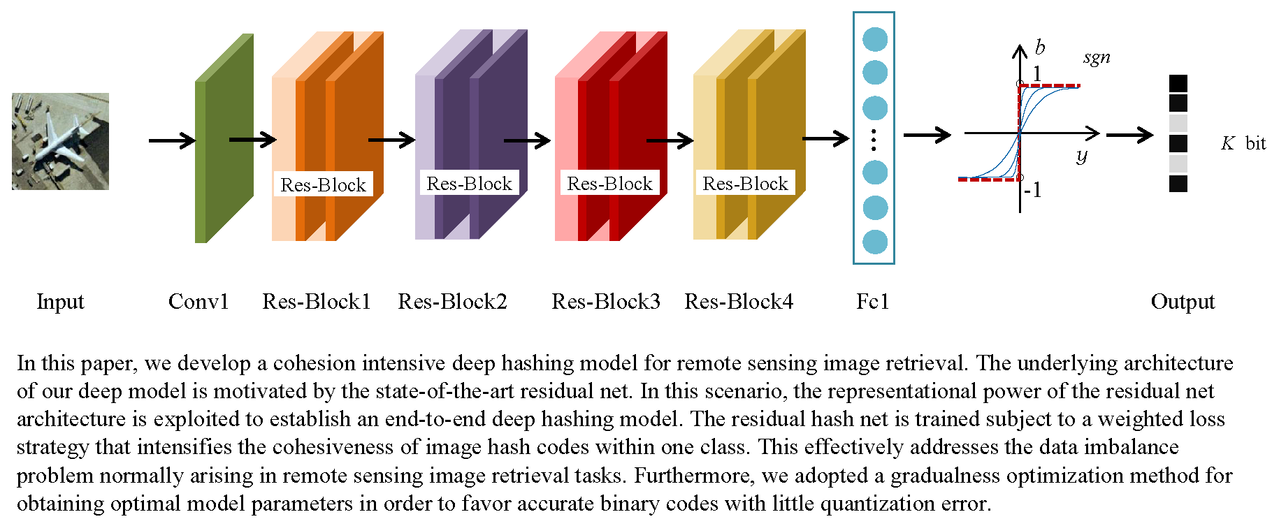
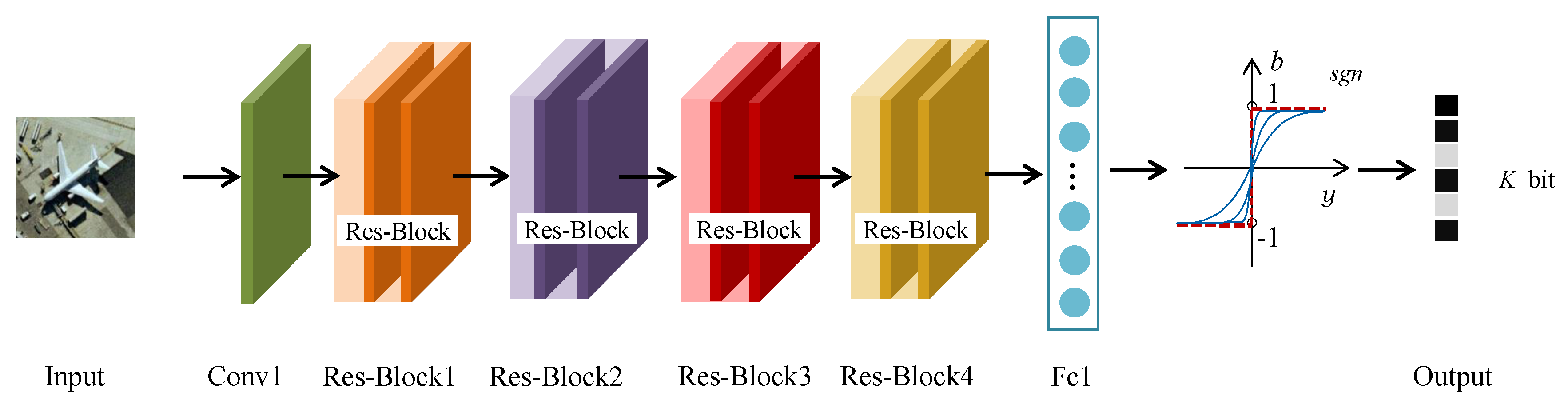
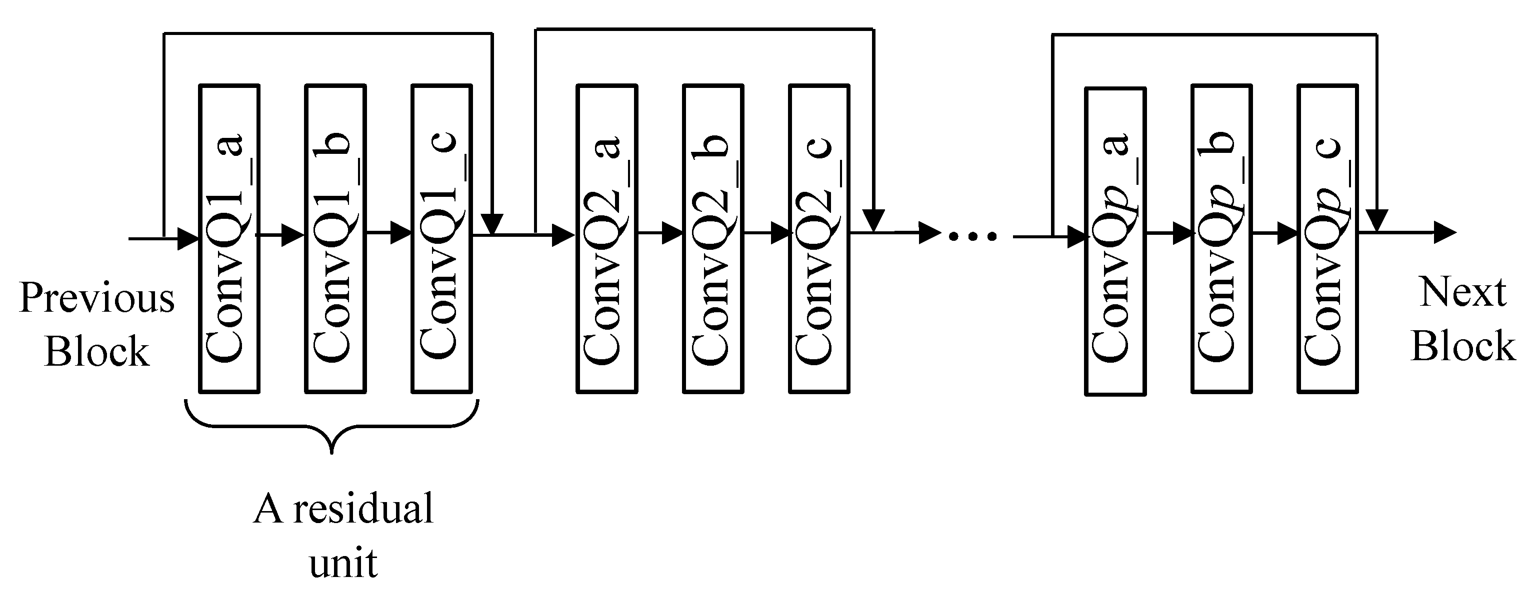
However, it is inappropriate to straightforwardly apply the residual net to hashing, because the outputs of the residual net are not binary codes but multiple class labels. For binarizing remote sensing images, we improve the residual net architecture and present a residual hash net whose outputs are binary codes, as shown in Figure 1. Similar to the residual net, our residual hash net consists of a convolutional layer (Conv1), four residual blocks (Res-Block1, Res-Block2, Res-Block3, Res-Block4), and a fully connected layer (Fc1). One residual block has a unique internal structure with several residual units and one residual unit has a certain number of convolutional layers, as shown in Figure 2. Different from the residual net, the fully connected layer of our residual hash net is activated by a Heaviside-like function and outputs K-bit binary codes for hashing. The architecture configuration of the residual hash net is specified in Table 1. The residual hash net comprehensively exploits the representational power of the residual net for the purpose of hashing remote sensing images.
Most existing deep hashing models use sigmoid as the activation function of the final fully connected layer, and are thus unable to output exact binary codes. Replacing the sigmoid by the Heaviside function is one approach to binary code generation.
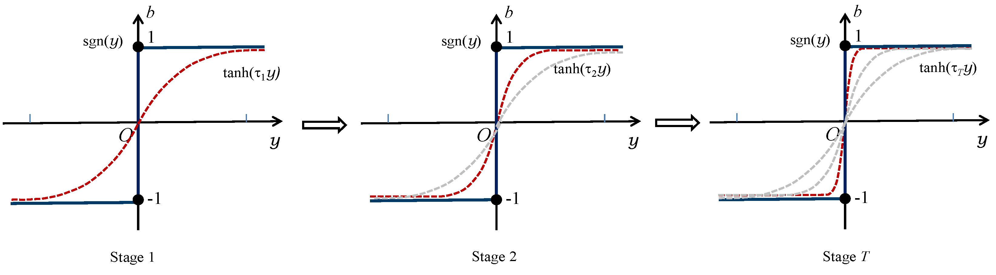
However, the Heaviside function is nonlinear and nonconvex, which may cause gradient vanishing in training the net with back propagation. To address this deficiency, we do not simply use the Heaviside function but exploit a Heaviside-like function. The gradualness optimization method [22] is used for approximating the Heaviside function. Specifically, we use the continuous function tanh() with a positive scaling parameter and the Fc1 output y for Heaviside approximation. As increases, tanh() gradually approaches sgn(y), as shown in Figure 3. The approximation is formulated as follows:
We commence the training procedure of the residual hash net by setting and training the network up to convergence. This accomplishes stage 1 in Figure 3. We then repetitively train the net up to convergence with respect to an increasing . This drives the Heaviside-like function to vary from stage 2 to stage T in Figure 3. Consequently, the residual hash net outputs accurate K bit hash codes of an image with little quantization error. We refer to the residual hash net along with the training strategy subject to the cohesion intensive loss function as the cohesion intensive deep hashing model.
2.2. Cohesion Intensive Loss Function
We describe how to develop loss functions for training the residual hash net presented in Section 2.1. For the image data set , we define as a common class indicator matrix. Specifically, for the ith and jth images, if , is 1 and 0 otherwise. The inner product is related to the Hamming distance. A big value reflects a small Hamming distance. The conditional of the common class indicator given the hash code pair is modeled in terms of multinomial logistic regression as follows:
The parameter is a normalized parameter to control the inner product value of and in the interval (−1, 1) when generating different length hash codes. In experiments, lambda is empirically set to be 1/K, where K is the length of hash codes. It does not affect the weight between different image pairs. When and are similar, a large value of is obtained, which leads to a large value of and vice versa.
Motivated by the continuation setting [22] for enhancing the intraclass similarity, we introduce a weight for a pair of remote sensing images and . Suppose that there are totally images belonging to the class , where the image is from. The weight between and is given as follows:
We formulate a weighted likelihood function as follows:
Based on (2) and (4), we have the loss function for training the residual hash net as follows:
where represents parameters of the residual hash net. The residual hash net is trained subject to minimizing (5) by updating . The weighting scheme enables the image similarities within one common class to play a more dominant role than those from different classes in the loss function. Specifically, the weight in (5) increases the loss for intraclass similar images. We refer to the loss function (5) as a cohesion intensive loss function. In a remote sensing data set, it is very common that the target image belongs to a class which only has a small proportion of images in the data set. This requires a retrieval algorithm to look for similar images from a big amount of almost irrelevant images. The data imbalance poses a big challenge for remote sensing image retrieval. The cohesion intensive loss function in turn neutralizes the data imbalance problem in terms of enhancing intraclass similarities.
3. Experimental Results
3.1. Experimental Setup
Land cover refers to the observed biological or physical cover on the earth’s surface (http://www.fao.org/3/x0596e/X0596e01e.htm). Strictly speaking, land cover should be limited to describing vegetation and manufactured cover. For example, Copernicus CORINE (https://land.copernicus.eu/pan-european/corine-land-cover) consists of an inventory of land cover in 44 classes. It has a wide variety of applications in many domains such as environment, agriculture, transport, and spatial planning. We use the two land-cover benchmark data sets, i.e., UCMerced and AID, in our work for experimental comparison. As commonly used remote sensing data sets for experimental evaluation, these two data sets comprise a number of geographic categories including natural and man-made land-cover. Experiments on these two data sets validate the effectiveness of the proposed CIDH in distinguishing a variety of geographical categories.
The UCMerced [23] data set was produced by the University of California. The data are images manually extracted from the US national maps of city areas, which were made by the US Geological Survey. It contains 21 land-cover classes and each land-cover class includes 100 images. Each image has 256×256 pixels. The image has a pixel resolution of one foot. In order to augment the UCMerced data set for extensive experimental evaluations, we rotate the original image by , , and , separately. The size of the UCMerced data set is then increased to 8400 images. We use 7400 images as training data and 1000 images as inquiry data. The data augmentation (e.g., rotation and flip) is very useful to explore the representational power of deep models for remote sensing image processing. It has been widely accepted that a deep model trained by an augmented training data set outperforms that by the original training data set for general remote sensing image analysis tasks [17].
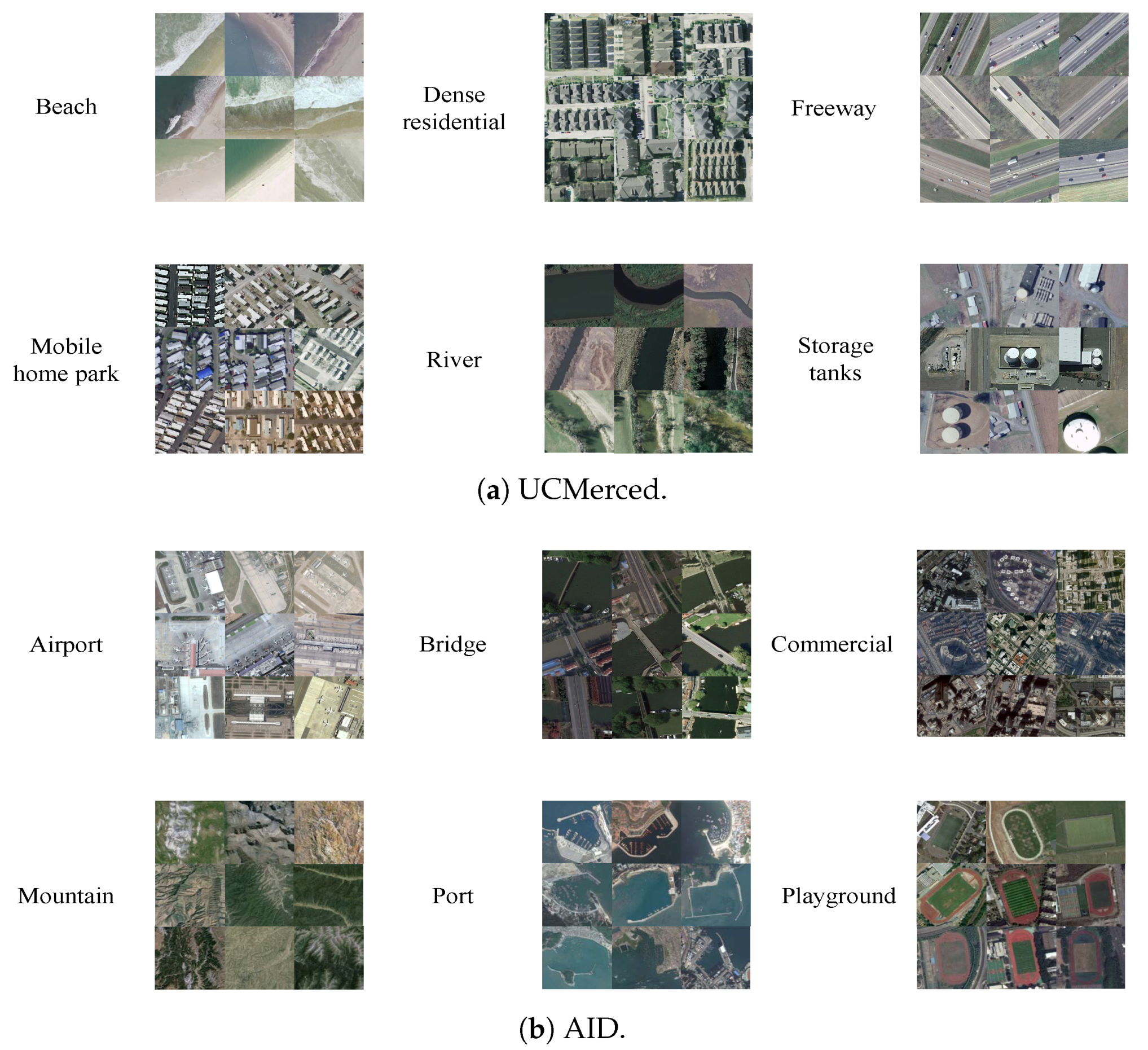
The AID [24] data set is a large-scale remote sensing image data set produced by Wuhan University in 2017. Images are collected from the Google Earth imagery, and labeled by specialists in the field of remote sensing image interpretation. Each image has 600×600 pixels. It has 30 classes of high-resolution images, and 200∼400 images for each class. We use 8000 images as training data and 2000 images as test data. Some examples of UCMerced and AID are shown in Figure 4.
Our CIDH model is implemented based on the open-source caffe framework (http://caffe.berkeleyvision.org/). We employ the residual net architecture [21], fine-tune a pretrained residual net model, and train a new layer Fc1 to produce hash codes. The metrics for evaluating retrieval accuracy are the mean average precision (MAP), the precision-recall (P-R) curve, and t-distributed Stochastic Neighbor Embedding (t-SNE) [25].
3.2. Results and Analysis
We compare the retrieval performance of CIDH with several shallow hashing methods, i.e., partial randomness hashing (PRH) [13], kernel-based supervised hashing (KSH) [12], supervised discrete hashing (SDH) [26], and column sampling-based discrete supervised hashing (COSDISH) [27]. The above methods are based on GIST features. In order to illustrate the advantages of the proposed CIDH model, we also compare it with the existing deep neural network models, including deep hashing network (DHN) [28], deep supervised hashing (DSH) [29], and deep hashing neural networks (DHNNs) [19]. The comparison deep hashing methods except DHNNs are reimplemented with open source code provided by the authors. All the parameter values are set to be those optimized by the original authors, resulting in favorable results expected by the authors. Additionally, we make comparison with the experimental results of DHNNs reported in the original paper. In order to make fair comparison, we follow the experimental settings of DHNNs. Especially, we set our data augmentation configuration to be the same with the state-of-the-art DHNNs, and the common experimental setting guarantees a fair comparison. The results are shown in Table 2.
In order to validate the gain of hashing methods in retrieval time, we have compared the efficiency of hashing-based retrieval and a hand-craft feature-based retrieval method. We use GIST [16] as the comparison hand-craft feature-based method. The GIST feature for one image is a 512-dimensional float value vector. In addition, we extract the GIST features and generate hash codes for each image in the database, separately. We measure the time of computing the distance between pairs of images, in terms of GIST features and hash codes, separately. The retrieval based on GIST features requires Euclidean distance with float value manipulations and that, based on hash codes, requires Hamming distance with binary operations. The retrieval time is shown in Table 2, where Time represents average retrieval time of one image. We observe that about 100 × Time is reduced by hashing retrieval instead of float value retrieval. The experiments validate the gain of hashing methods over feature-based retrieval methods in retrieval time.
PRH, KSH, SDH, and COSDISH are hash algorithms based on hand-craft features, and the others are hash algorithms based on deep neural networks. We observe in Table 2 that the performance of the hash algorithms based on deep neural networks is far superior to those based on hand-craft features, and our CIDH achieves the best performance. This is because the deep hash algorithms couple the feature extraction and hashing, encouraging these two processes to adapt to each other. As the latest remote sensing image retrieval hashing method, DHNNs use the uniform loss weights and thus does not address the data-imbalance problem. Our CIDH exploits a specific weighting strategy to balance the loss of different image pairs. The specific weights make the image loss of the common class larger than that of different classes. Therefore, the hash codes generated by the common class of images are encouraged to be closer. This enables our model to outperform DHNNs.
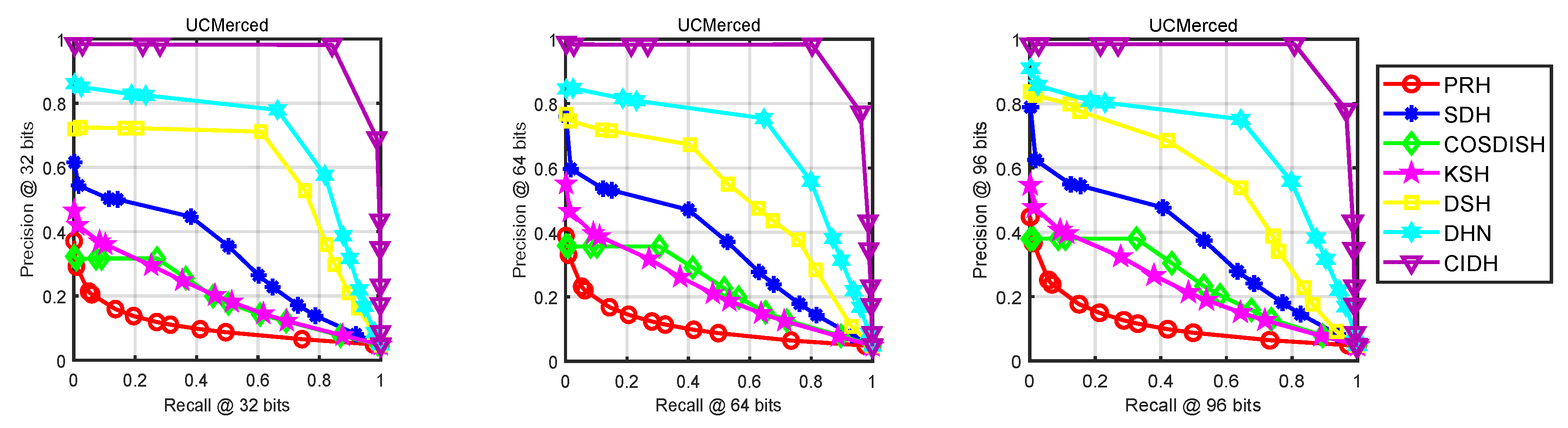
In order to further illustrate the performance results of remote sensing image retrieval, we draw the P-R curves of CIDH and competing deep neural network approaches. Here, both the coverage of retrieval results and the ordering of retrieval results are considered. Figure 5 shows the P-R curves of the methods based on different hash code lengths. At the same recall rate, the accuracy of our method is significantly higher than the three competitor methods. Similarly, the recall rate of our method is significantly higher than the other methods at the same accuracy rate. As shown in Figure 5, CIDH is superior to other methods in terms of both accuracy and recall.
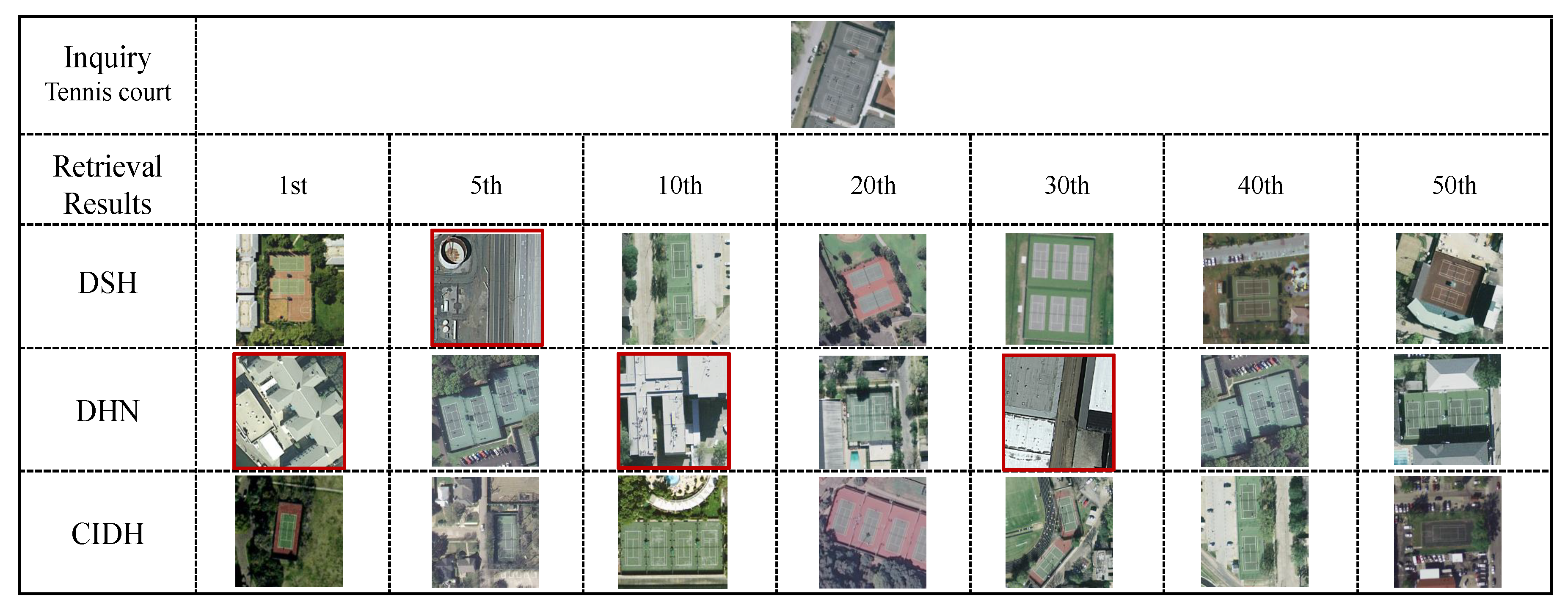
In addition, we present a visual comparison of deep hashing methods in Figure 6—the 1st, 5th, 10th, 20th, 30th, 40th, and 50th retrieval results are shown. In order to demonstrate the cohesion intensive properties of CIDH, a tennis court image is used as the inquiry image. The appearance of such images is very similar to other classes (such as buildings), and it is easy for retrieval algorithms to fail. It is observed that DHN and DSH retrieve several false images. On the other hand, our cohesion intensive loss function ensures that the hash codes of different images within one class are as similar as possible. In addition, the tennis court images with different rotations are correctly retrieved by our CIDH. This validates again that the retrieval result of CIDH is significantly better than other methods.
We also perform experiments on the AID data set. Table 3 shows the results on AID with different hash code lengths. The number of images in each class in the AID data set is different from one another. Our cohesion intensive loss addresses this variability, and our CIDH performs the best on AID data set. The P-R curves on AID (shown in Figure 7) validate that our method achieves superior performance.
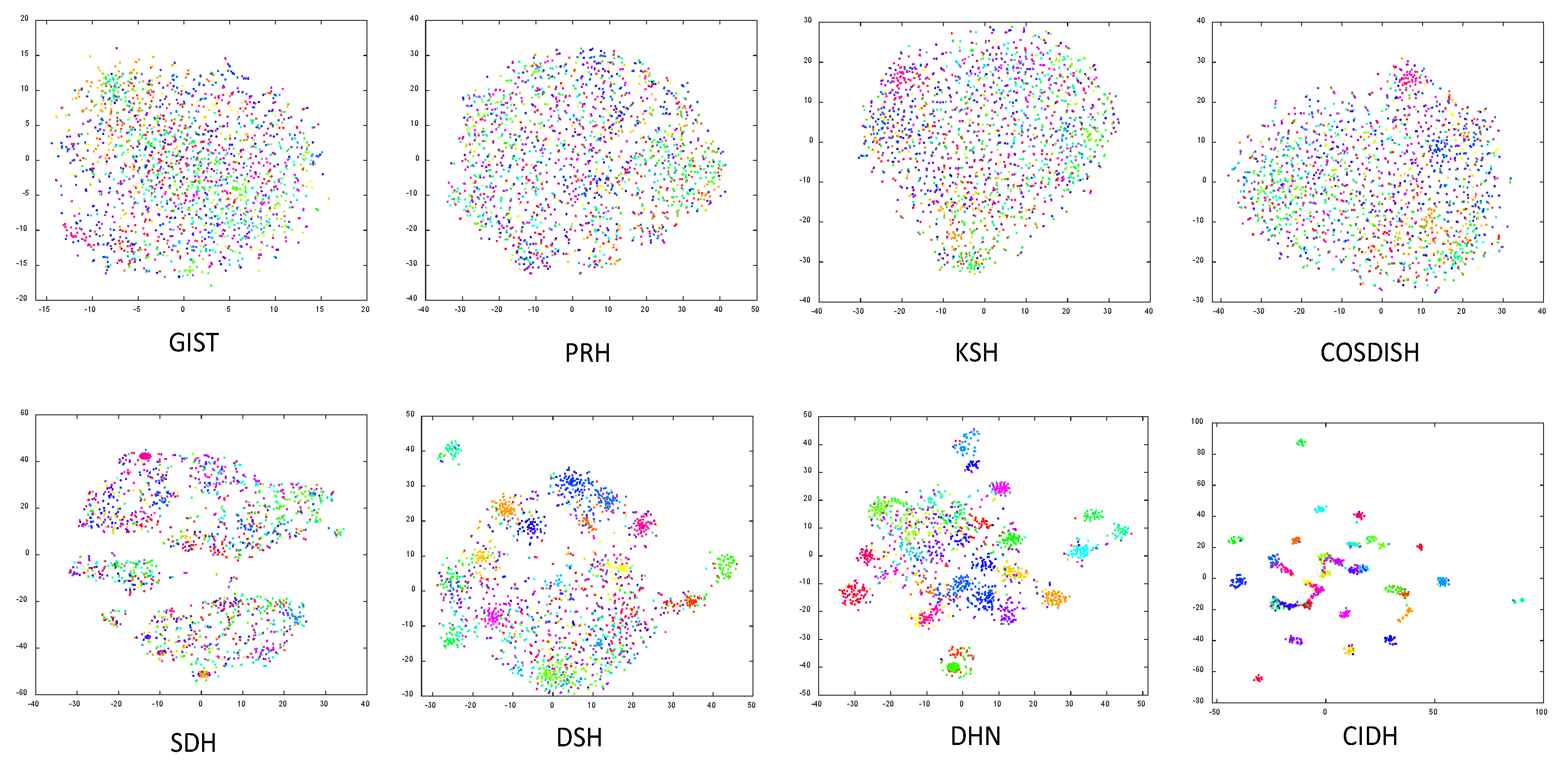
In addition, in order to demonstrate the cohesion enhancement proposed by CIDH, we visualize the t-SNE of the hash codes generated by comparison methods on the AID data set in Figure 8. As we have described above, the AID data set not only contains more geographical categories than the UCMerced data set, but also each category includes a different number of images. Thus, it is challenging to cohere hash codes from the same class of images. According to Figure 8, we observe that the hash codes learning by CIDH has discriminative distribution, and each category is well separated. However, the hash codes learning by comparison methods do not have such discriminative distribution and a considerable number of different category hash codes are mixed up. The t-SNE results suggest that our CIDH better brings together hash codes generated by the same category images than comparison methods.
The above experimental results verify that our method has superior performance on large-scale remote sensing data sets.
We have released our code for public evaluation (https://github.com/lrhan/CIDH-caffe).
4. Conclusions
We have developed a cohesion intensive deep hashing model for remote sensing image retrieval. We have initially developed a residual hash net for binarizing remote sensing images. The proposed residual hash net learns accurate binary hash codes by optimizing a novel cohesion intensive loss function. This ensures that the hash codes of different images within one class are as similar as possible. The residual hash net is then effectively trained, subject to gradualness optimization, which favors accurate binary codes with little quantization error. We have conducted comparative experiments on extensively large remote sensing data sets such as UCMerced and AID. The experiments clearly show the effectiveness of the proposed model compared with other state-of-the-art models.
The visual features for remote sensing images from different categories are quite different. For example, the urban views have rich visual features while the rural landscapes have rare visual features. Most deep learning models address these differences in an indiscriminative manner. It is worth improving the CIDH by considering different visual features from different categories.
Author Contributions
L.H., P.L. and P.R. conceived and designed the experiments; L.H. performed the experiments; L.H., X.B., C.G. and X.Z. analyzed the data; C.G. polished the paper; and L.H. wrote the paper. All authors have read and agreed to the published version of the manuscript.
Funding
This research was funded by the National Key R&D Program of China under Project 2017YFC1405600, National Natural Science Foundation of China under Project 61602517, Shandong Provincial Key R&D Program under Project 2017CXGC0902, and Research Fund for the Creative Research Team of Young Scholars at Universities in Shandong Province under Grant No. 2019KJN019.
Conflicts of Interest
The authors declare no conflict of interest.
References
- Wang, Q.; Gao, J.; Yuan, Y. Embedding Structured Contour and Location Prior in Siamesed Fully Convolutional Networks for Road Detection. IEEE Trans. Intell. Transp. Syst. 2018, 19, 230–241. [Google Scholar] [CrossRef] [Green Version]
- Ma, J.; Zhou, H.; Zhao, J.; Gao, Y.; Jiang, J.; Tian, J. Robust feature matching for remote sensing image registration via locally linear transforming. IEEE Trans. Geosci. Remote Sens. 2015, 53, 6469–6481. [Google Scholar] [CrossRef]
- Ma, J.; Zhao, J.; Jiang, J.; Zhou, H.; Guo, X. Locality preserving matching. Int. J. Comput. Vis. 2019, 127, 512–531. [Google Scholar] [CrossRef]
- Li, Y.; Tao, C.; Tan, Y.; Shang, K.; Tian, J. Unsupervised Multilayer Feature Learning for Satellite Image Scene Classification. IEEE Geosci. Remote Sens. Lett. 2016, 13, 157–161. [Google Scholar] [CrossRef]
- Li, Y.; Zhang, Y.; Huang, X.; Yuille, A.L. Deep networks under scene-level supervision for multi-class geospatial object detection from remote sensing images. Isprs J. Photogramm. Remote Sens. 2018, 146, 182–196. [Google Scholar] [CrossRef]
- Patil, R.; Sharma, S.K.; Tignath, S. Remote Sensing and GIS based soil erosion assessment from an agricultural watershed. Arab. J. Geosci. 2015, 8, 6967–6984. [Google Scholar] [CrossRef]
- Wang, J.; Kumar, S.; Chang, S.F. Semi-supervised hashing for scalable image retrieval. In Proceedings of the IEEE Conference on Computer Vision and Pattern Recognition, San Francisco, CA, USA, 13–18 June 2010. [Google Scholar]
- Datar, M.; Immorlica, N.; Indyk, P.; Mirrokni, V.S. Locality-sensitive hashing scheme based on p-stable distributions. Symp. Comput. Geom. 2004, 8–11, 253–262. [Google Scholar]
- Weiss, Y.; Torralba, A.; Fergus, R. Spectral Hashing. Neural Inf. Process. Syst. 2008, 8–11, 1753–1760. [Google Scholar]
- Gong, Y.; Lazebnik, S. Iterative quantization: A procrustean approach to learning binary codes. IEEE Trans. Pattern Anal. Mach. Intell. 2012, 35, 2916–2929. [Google Scholar] [CrossRef] [PubMed] [Green Version]
- Lukac, N.; Zalik, B.; Cui, S.; Datcu, M. GPU-based kernelized locality-sensitive hashing for satellite image retrieval. In Proceedings of the 2015 IEEE International Geoscience and Remote Sensing Symposium (IGARSS), Milan, Italy, 26–31 July 2015; pp. 1468–1471. [Google Scholar]
- Demir, B.; Bruzzone, L. Hashing-Based Scalable Remote Sensing Image Search and Retrieval in Large Archives. IEEE Trans. Geosci. Remote Sens. 2016, 54, 892–904. [Google Scholar] [CrossRef]
- Li, P.; Ren, P. Partial Randomness Hashing for Large-Scale Remote Sensing Image Retrieval. IEEE Geosci. Remote Sens. Lett. 2017, 14, 464–468. [Google Scholar] [CrossRef]
- Li, P.; Zhang, X.; Zhu, X.; Ren, P. Online Hashing for Scalable Remote Sensing Image Retrieval. Remote Sens. 2018, 10, 709. [Google Scholar] [CrossRef] [Green Version]
- Lowe, D.G. Distinctive Image Features from Scale-Invariant Keypoints. Int. J. Comput. Vis. 2004, 60, 91–110. [Google Scholar] [CrossRef]
- Oliva, A.; Torralba, A. Modeling the Shape of the Scene: A Holistic Representation of the Spatial Envelope. Int. J. Comput. Vis. 2001, 42, 145–175. [Google Scholar] [CrossRef]
- Yu, X.; Wu, X.; Luo, C.; Peng, R. Deep learning in remote sensing scene classification: A data augmentation enhanced convolutional neural network framework. Gisci. Remote Sens. 2017, 54, 741–758. [Google Scholar] [CrossRef] [Green Version]
- Xie, M.; Jean, N.; Burke, M.; Lobell, D.; Ermon, S. Transfer Learning from Deep Features for Remote Sensing and Poverty Mapping. In Proceedings of the Thirtieth AAAI Conference on Artificial Intelligence, Phoenix, AZ, USA, 12–17 February 2016. [Google Scholar]
- Li, Y.; Zhang, Y.; Huang, X.; Zhu, H.; Ma, J. Large-Scale Remote Sensing Image Retrieval by Deep Hashing Neural Networks. IEEE Trans. Geosci. Remote Sens. 2018, 56, 950–965. [Google Scholar] [CrossRef]
- Li, Y.; Zhang, Y.; Huang, X.; Ma, J. Learning Source-Invariant Deep Hashing Convolutional Neural Networks for Cross-Source Remote Sensing Image Retrieval. IEEE Trans. Geosci. Remote Sens. 2018, 56, 6521–6536. [Google Scholar] [CrossRef]
- He, K.; Zhang, X.; Ren, S.; Sun, J. Deep Residual Learning for Image Recognition. In Proceedings of the Computer Vision and Pattern Recognition, Las Vegas, NV, USA, 26 June–1 July 2015. [Google Scholar]
- Cao, Z.; Long, M.; Wang, J.; Yu, P.S. HashNet: Deep Learning to Hash by Continuation. In Proceedings of the IEEE International Conference on Computer Vision (ICCV), Venice, Italy, 22–29 October 2017; pp. 5609–5618. [Google Scholar]
- Yang, Y.; Newsam, S.D. Bag-of-visual-words and spatial extensions for land-use classification. In Proceedings of the 18th SIGSPATIAL International Conference on Advances in Geographic Information Systems, San Jose, CA, USA, 2–5 November 2010; pp. 270–279. [Google Scholar]
- Xia, G.S.; Hu, J.; Fan, H.; Shi, B.; Xiang, B.; Zhong, Y.; Zhang, L. AID: A Benchmark Dataset for Performance Evaluation of Aerial Scene Classification. IEEE Trans. Geosci. Remote Sens. 2017, 55, 3965–3981. [Google Scholar] [CrossRef] [Green Version]
- Donahue, J.; Jia, Y.; Vinyals, O.; Hoffman, J.; Zhang, N.; Tzeng, E.; Darrell, T. DeCAF: A Deep Convolutional Activation Feature for Generic Visual Recognition. In Proceedings of the International Conference on Machine Learning 2014, Beijing, China, 21–26 June 2014. [Google Scholar]
- Shen, F.; Shen, C.; Liu, W.; Shen, H.T. Supervised Discrete Hashing. In Proceedings of the Computer Vision and Pattern Recognition, Boston, MA, USA, 7–12 June 2015; pp. 37–45. [Google Scholar]
- Kang, W.; Li, W.; Zhou, Z. Column sampling based discrete supervised hashing. In Proceedings of the AAAI Conference on Artificial Intelligence 2016, Phoenix, AZ, USA, 12–17 February 2016; pp. 1230–1236. [Google Scholar]
- Zhu, H.; Long, M.; Wang, J.; Cao, Y. Deep Hashing Network for efficient similarity retrieval. In Proceedings of the AAAI Conference on Artificial Intelligence 2016, Phoenix, AZ, USA, 12–17 February 2016; pp. 2415–2421. [Google Scholar]
- Liu, H.; Wang, R.; Shan, S.; Chen, X. Deep Supervised Hashing for Fast Image Retrieval. In Proceedings of the Computer Vision and Pattern Recognition 2016, Las Vegas, NV, USA, 26 June–1 July 2016; pp. 2064–2072. [Google Scholar]
Figure 1.
The residual hash net consists of a convolutional layer (Conv1), four residual blocks (Res-Block1, Res-Block2, Res-Block3, Res-Block4), and a fully connected layer (Fc1). A Heaviside-like function plays the role of the activation function for binarizing the outputs of Fc1. One input of the network is a remote sensing image, and the corresponding output is a piece of K-bit binary code for the image.

Figure 2.
A residual block: Res-BlockQ {Q = 1,2,3,4} represents a residual block, which consists of p residual units. For Res-Block1, Res-Block2, Res-Block3, and Res-Block4, p is 3, 4, 6, 3, respectively. A residual unit contains three convolution layers. A residual unit takes both the input and output of its previous residual unit as the inputs.

Figure 3.
The process of gradually approaching sgn(y) as increases, where .

Figure 4.
Illustration of UCMerced and AID data set. UCMerced contains 21 geography classes and each class has 100 images. We give some examples of several classes. AID contains 30 geography classes and each class has 200∼400 images. We give some examples of several classes of both data sets.
Figure 4.
Illustration of UCMerced and AID data set. UCMerced contains 21 geography classes and each class has 100 images. We give some examples of several classes. AID contains 30 geography classes and each class has 200∼400 images. We give some examples of several classes of both data sets.

Figure 5.
The precision-recall (P-R) curves of deep methods on UCMerced data set.

Figure 6.
Visual image retrieval results of different deep methods examined with 32 bits. The 1st, 5th, 10th, 20th, 30th, 40th, and 50th retrieval results are shown. In addition, false retrieval results are marked with red rectangles.
Figure 6.
Visual image retrieval results of different deep methods examined with 32 bits. The 1st, 5th, 10th, 20th, 30th, 40th, and 50th retrieval results are shown. In addition, false retrieval results are marked with red rectangles.

Figure 7.
The P-R curves of deep methods on AID data set.

Figure 8.
The t-distributed Stochastic Neighbor Embedding (t-SNE) of different length hash codes generated by comparison methods on AID data set.
Figure 8.
The t-distributed Stochastic Neighbor Embedding (t-SNE) of different length hash codes generated by comparison methods on AID data set.


Table 1.
Residual hash net configuration.
| Layer | Configuration |
|---|---|
| Conv1 | , 64, Stride 2 |
| Res-Block1 | |
| Res-Block2 | |
| Res-Block3 | |
| Res-Block4 | |
| Fc1 |
Table 2.
Mean average precision (MAP) and average retrieval time (s) of comparison methods on UCMerced data set.
Table 2.
Mean average precision (MAP) and average retrieval time (s) of comparison methods on UCMerced data set.
| Method | GIST | PRH | KSH | COSDISH | SDH | DSH | DHN | DHNNs | CIDH | ||
|---|---|---|---|---|---|---|---|---|---|---|---|
| Bits | mAP | Time | mAP | Time | mAP | mAP | mAP | mAP | mAP | mAP | mAP |
| K = 32 | 0.4672 | 0.022907 | 0.3361 | 0.000846 | 0.4609 | 0.3235 | 0.5943 | 0.6327 | 0.6768 | 0.9396 | 0.9846 |
| K = 64 | 0.4672 | 0.022907 | 0.3667 | 0.000927 | 0.5049 | 0.3631 | 0.6551 | 0.6831 | 0.7423 | 0.9718 | 0.9853 |
| K = 96 | 0.4672 | 0.022907 | 0.4015 | 0.000971 | 0.5114 | 0.3840 | 0.6809 | 0.7342 | 0.7867 | 0.9762 | 0.9858 |
Table 3.
MAP and average retrieval time (s) of comparison methods on AID data set.
| Method | GIST | PRH | KSH | COSDISH | SDH | DSH | DHN | DHNNs | CIDH | ||
|---|---|---|---|---|---|---|---|---|---|---|---|
| Bits | mAP | Time | mAP | Time | mAP | mAP | mAP | mAP | mAP | mAP | mAP |
| K = 32 | 0.2439 | 0.040966 | 0.1816 | 0.000801 | 0.2164 | 0.1988 | 0.2444 | 0.4191 | 0.6953 | - | 0.8780 |
| K = 64 | 0.2439 | 0.040966 | 0.2051 | 0.000872 | 0.2492 | 0.2245 | 0.3285 | 0.4585 | 0.7464 | - | 0.9043 |
| K = 96 | 0.2439 | 0.040966 | 0.2199 | 0.000946 | 0.2599 | 0.2158 | 0.2599 | 0.4636 | 0.7682 | - | 0.9245 |
© 2019 by the authors. Licensee MDPI, Basel, Switzerland. This article is an open access article distributed under the terms and conditions of the Creative Commons Attribution (CC BY) license (http://creativecommons.org/licenses/by/4.0/).
Share and Cite
MDPI and ACS Style
Han, L.; Li, P.; Bai, X.; Grecos, C.; Zhang, X.; Ren, P. Cohesion Intensive Deep Hashing for Remote Sensing Image Retrieval. Remote Sens. 2020, 12, 101. https://0-doi-org.brum.beds.ac.uk/10.3390/rs12010101
AMA Style
Han L, Li P, Bai X, Grecos C, Zhang X, Ren P. Cohesion Intensive Deep Hashing for Remote Sensing Image Retrieval. Remote Sensing. 2020; 12(1):101. https://0-doi-org.brum.beds.ac.uk/10.3390/rs12010101
Chicago/Turabian StyleHan, Lirong, Peng Li, Xiao Bai, Christos Grecos, Xiaoyu Zhang, and Peng Ren. 2020. "Cohesion Intensive Deep Hashing for Remote Sensing Image Retrieval" Remote Sensing 12, no. 1: 101. https://0-doi-org.brum.beds.ac.uk/10.3390/rs12010101
Note that from the first issue of 2016, this journal uses article numbers instead of page numbers. See further details here.