Flash-Flood Susceptibility Assessment Using Multi-Criteria Decision Making and Machine Learning Supported by Remote Sensing and GIS Techniques

 ,
, 
 , , , ,
Abstract
:
1. Introduction
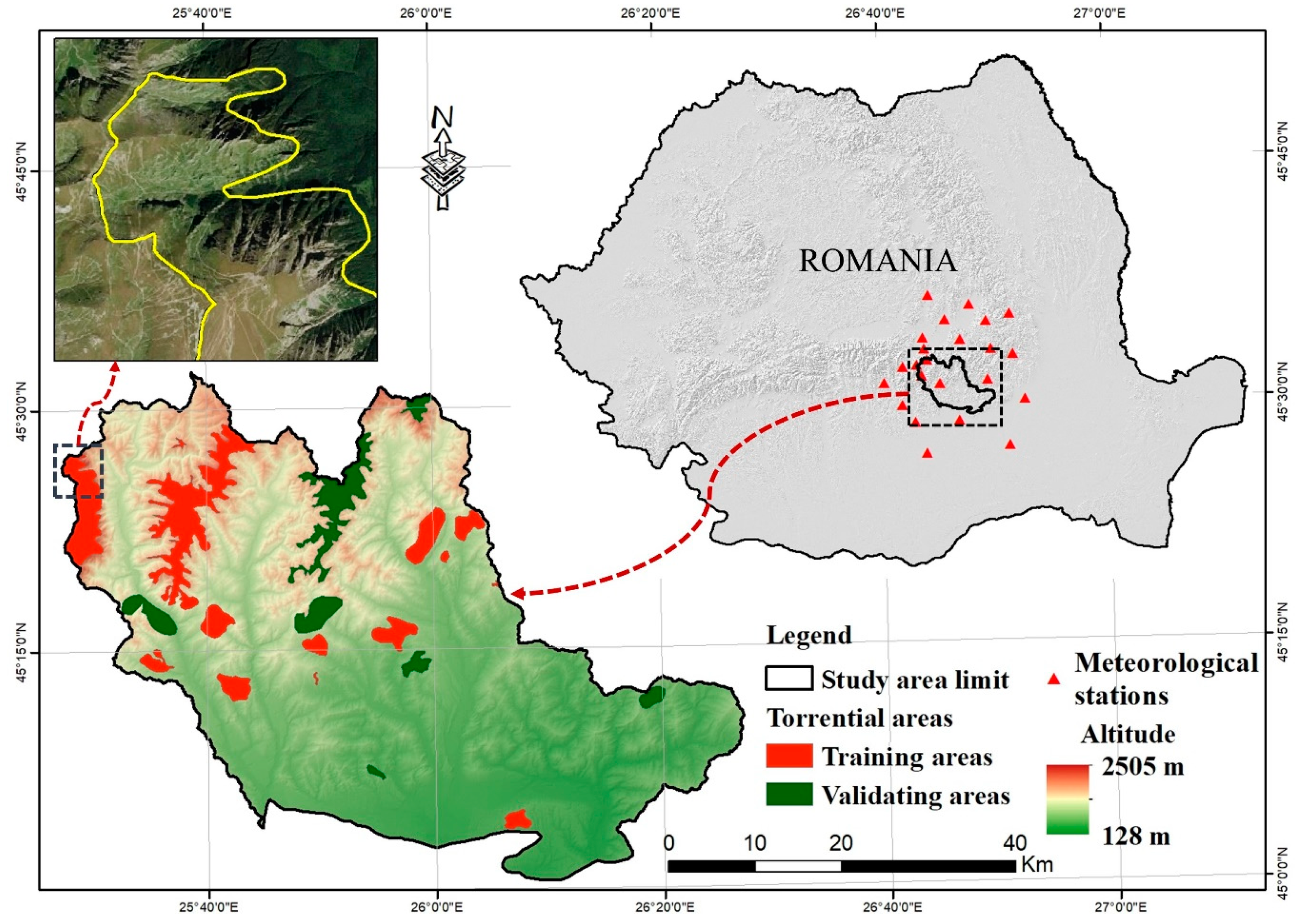
2. Study Area
3. Data
3.1. Inventory of Torrential Areas
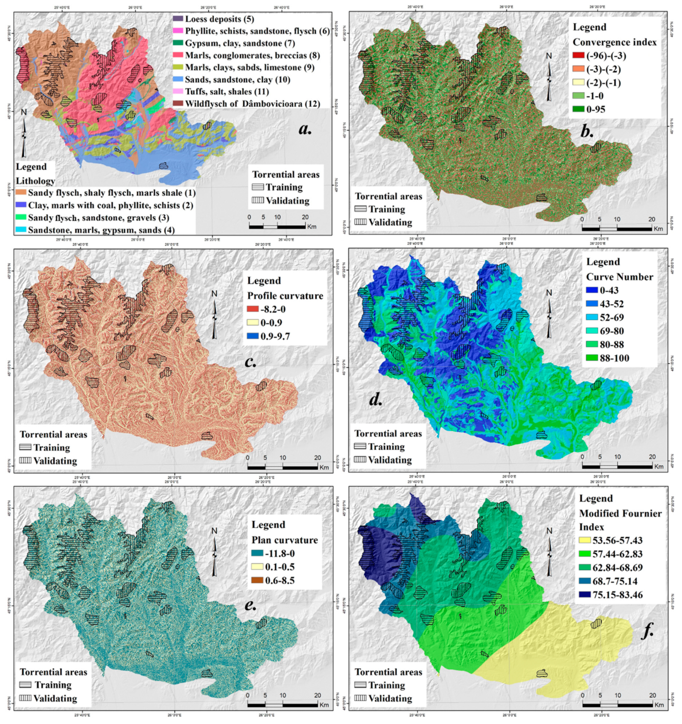
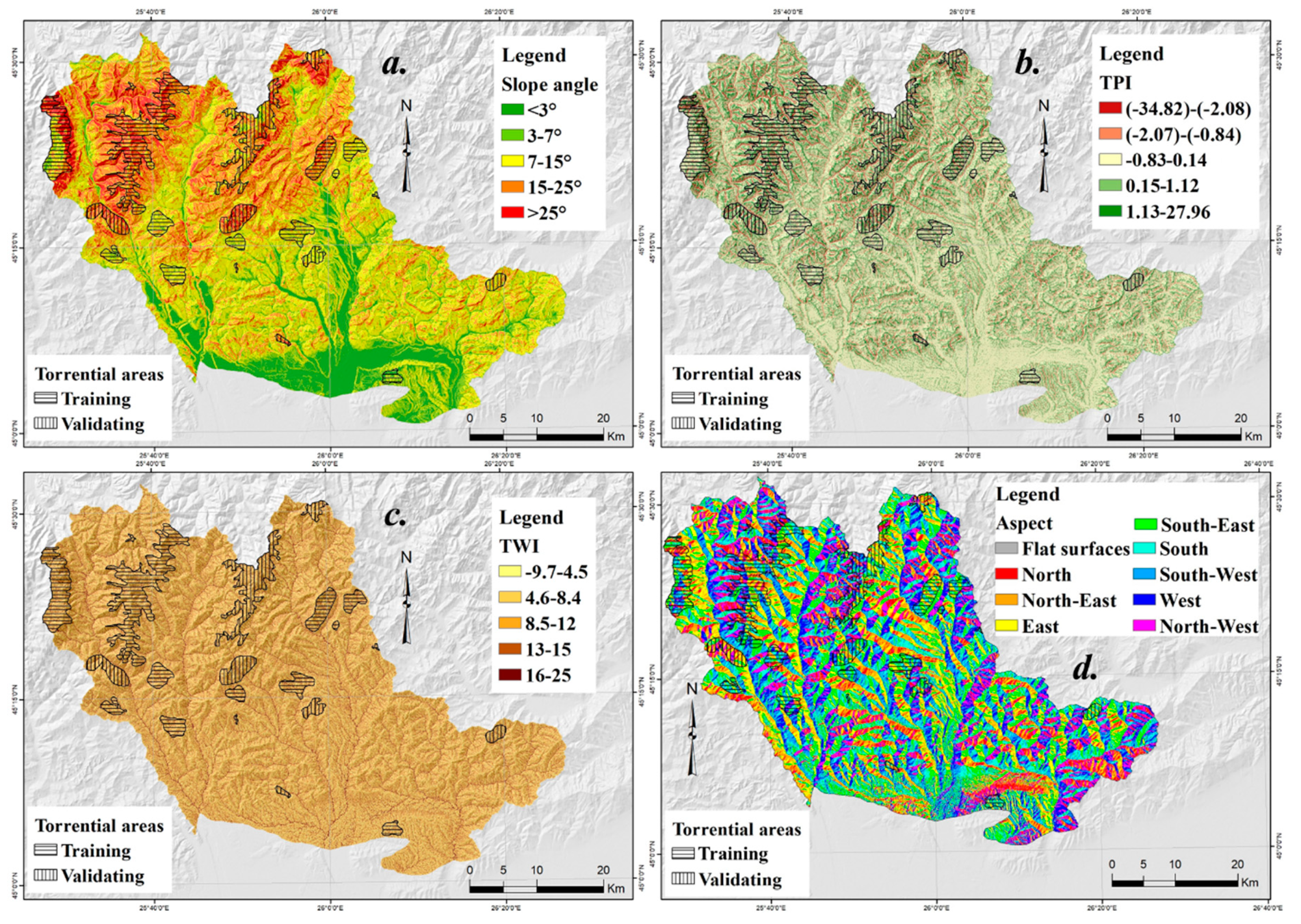
3.2. Flash-Flood Conditioning Factors
4. Background of the Employed Algorithms
4.1. Analytical Hierarchy Process (AHP)
4.2. k-Nearest Neighbor (kNN)
4.3. Lazy K-Star (KS) Algorithm
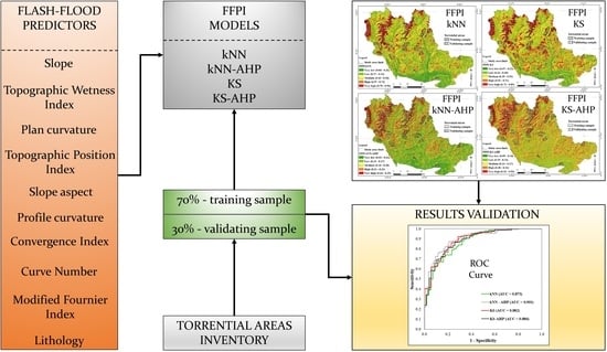
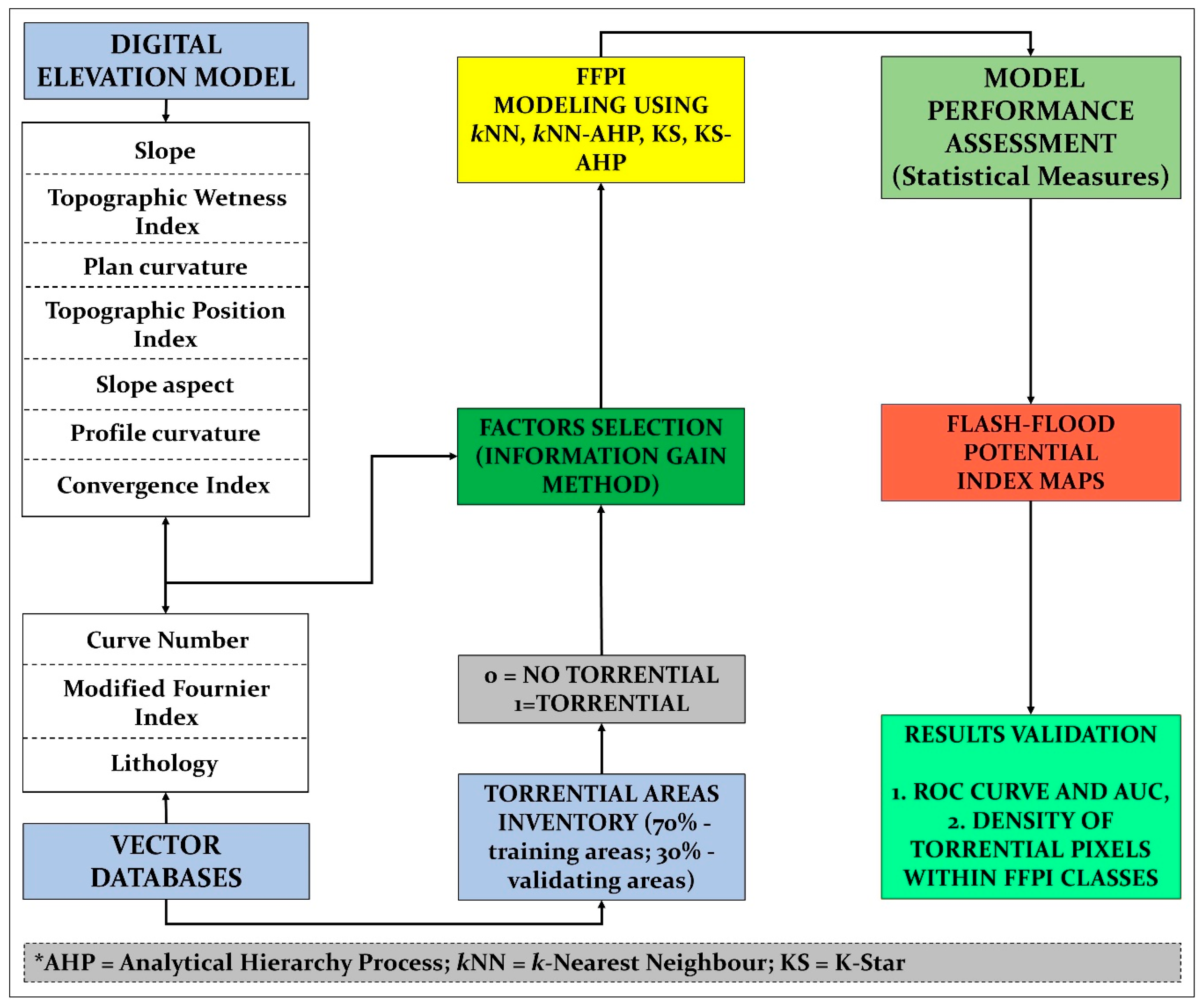
5. Proposed Methodology for Predicting Flash-Flood Potential
5.1. Establishment of Flash-Flood Database
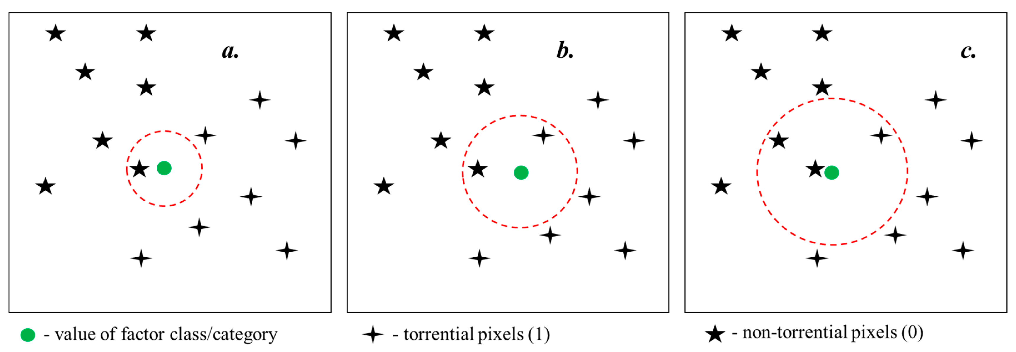
5.2. Selection of Flash-Flood Predictors Applying Information Gain Ratio (IGR) Method
5.3. Computing the AHP Weights for Factor Classes/Categories
5.4. Training and Validation Dataset Preparation
5.5. Configuration and Training of Flash-Flood Potential Models
5.6. Evaluation of the Model Performance
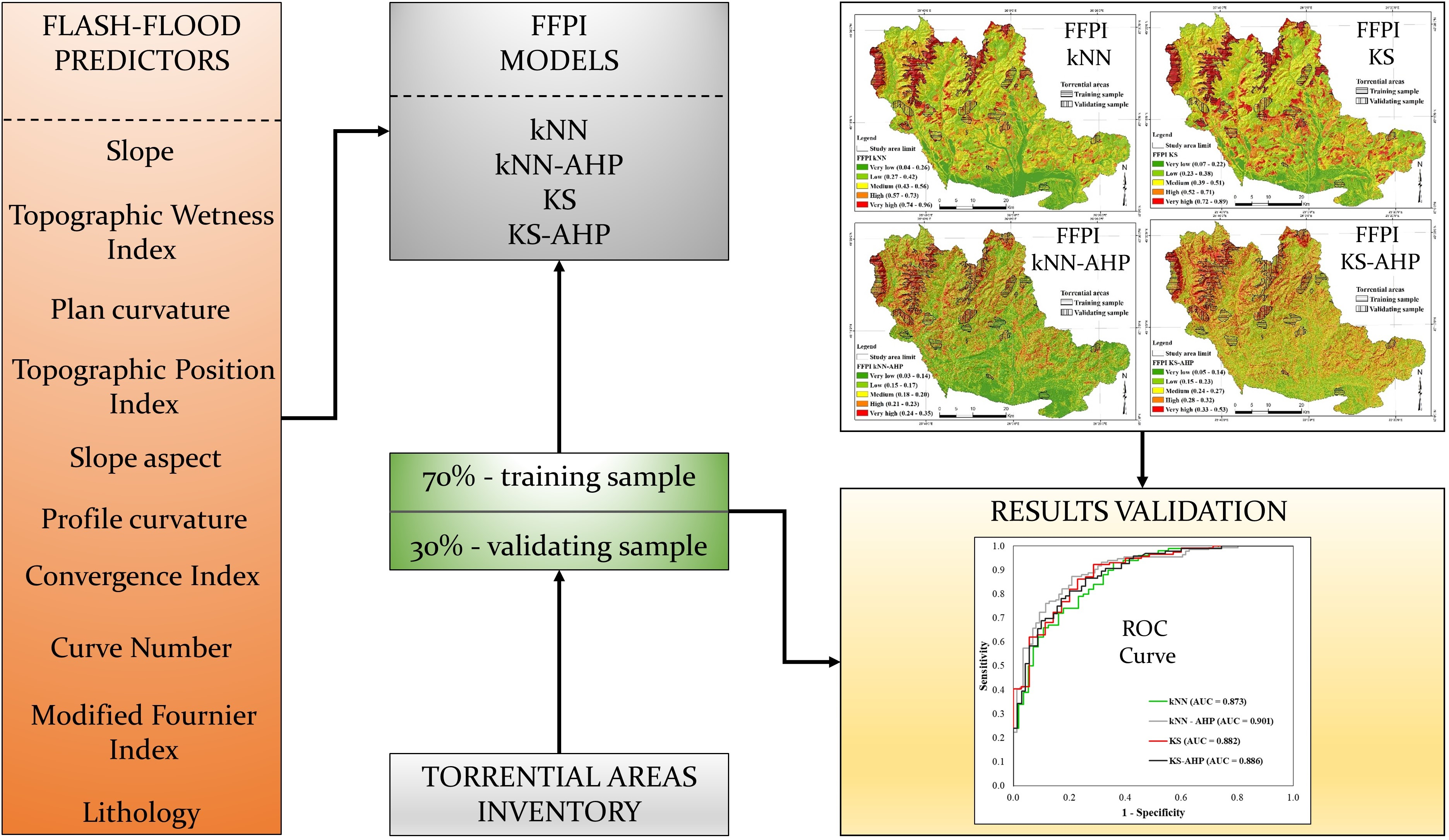
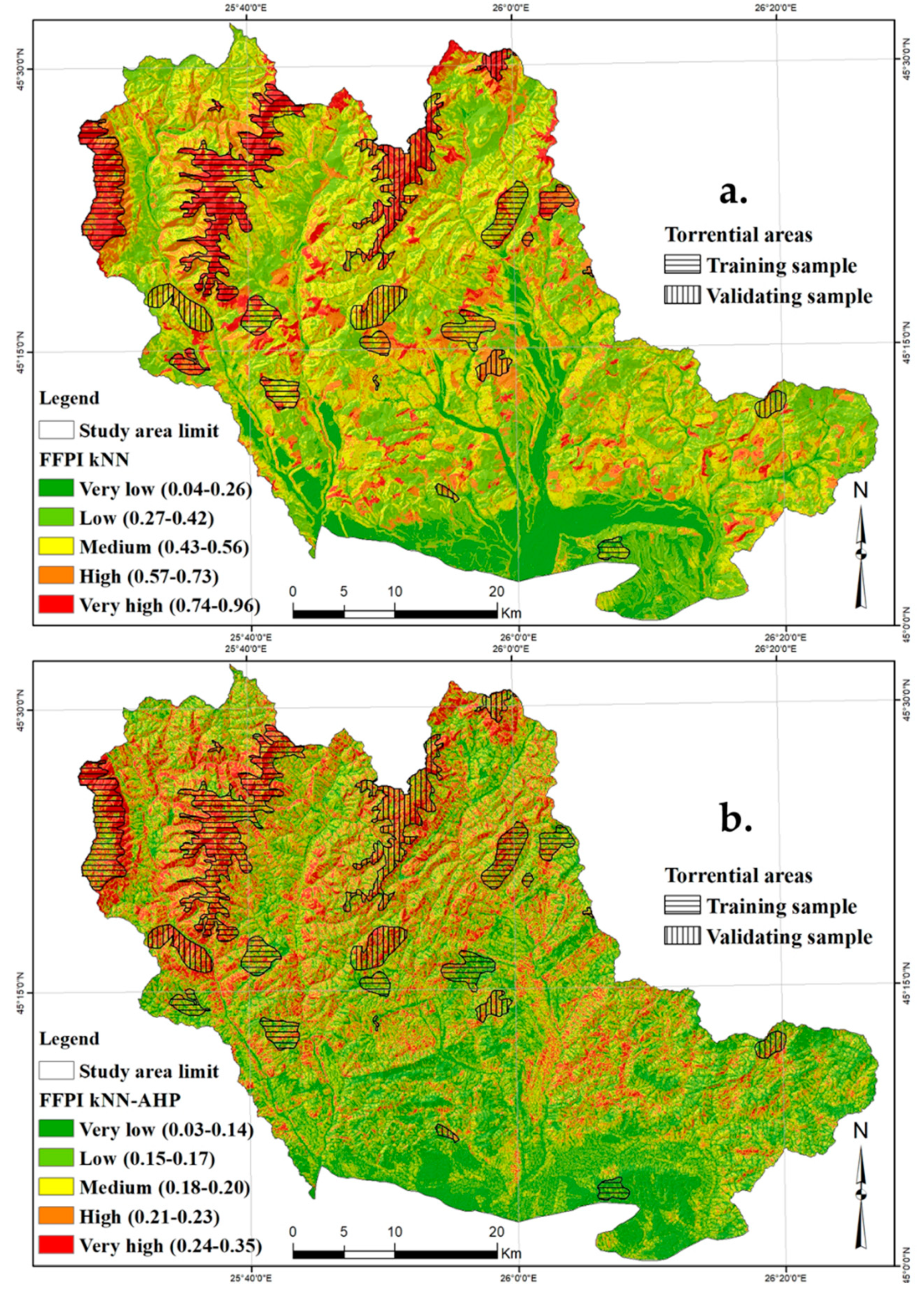
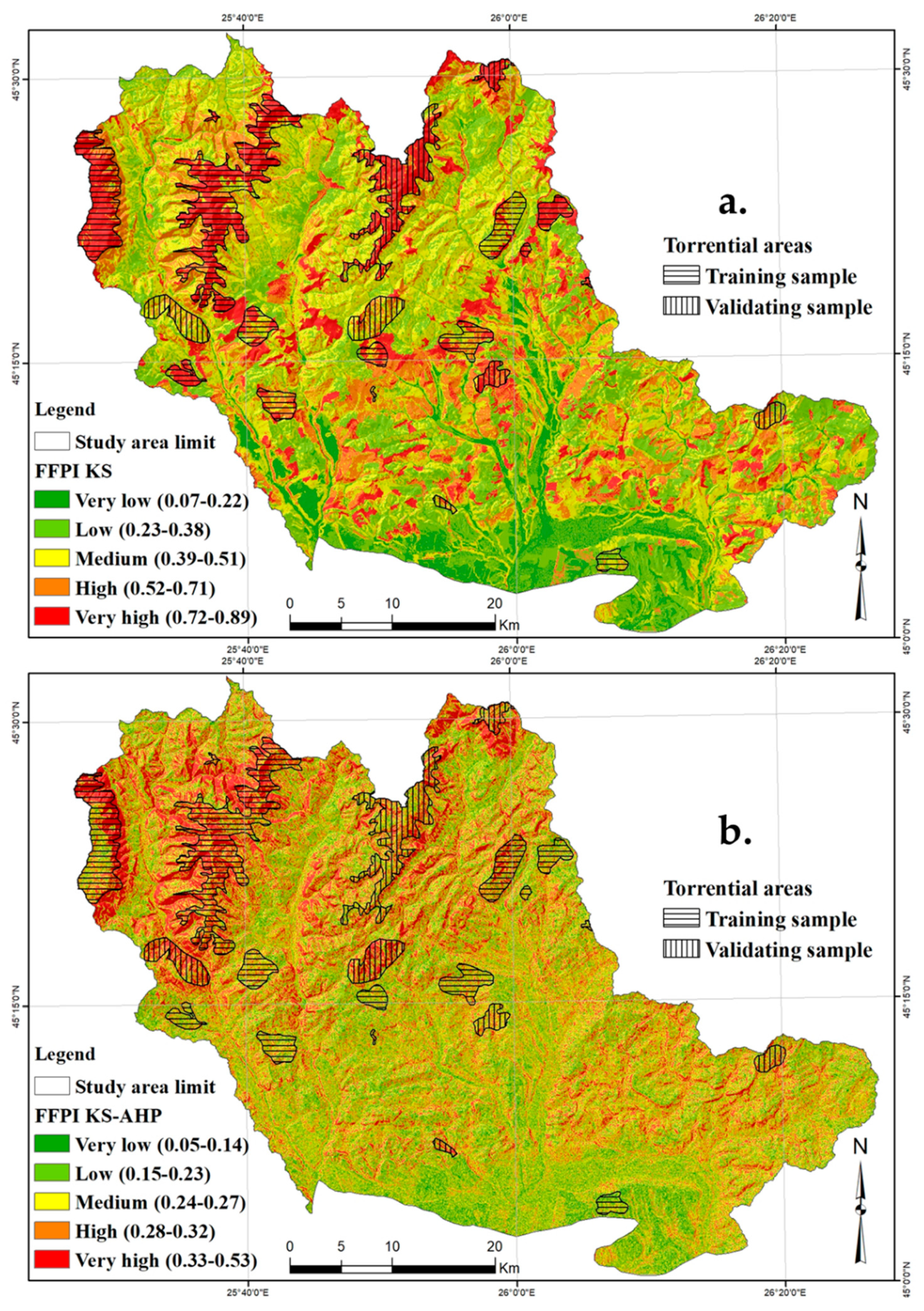
5.7. Flash-Flood Potential Mapping and Results Validation
6. Results and Discussion
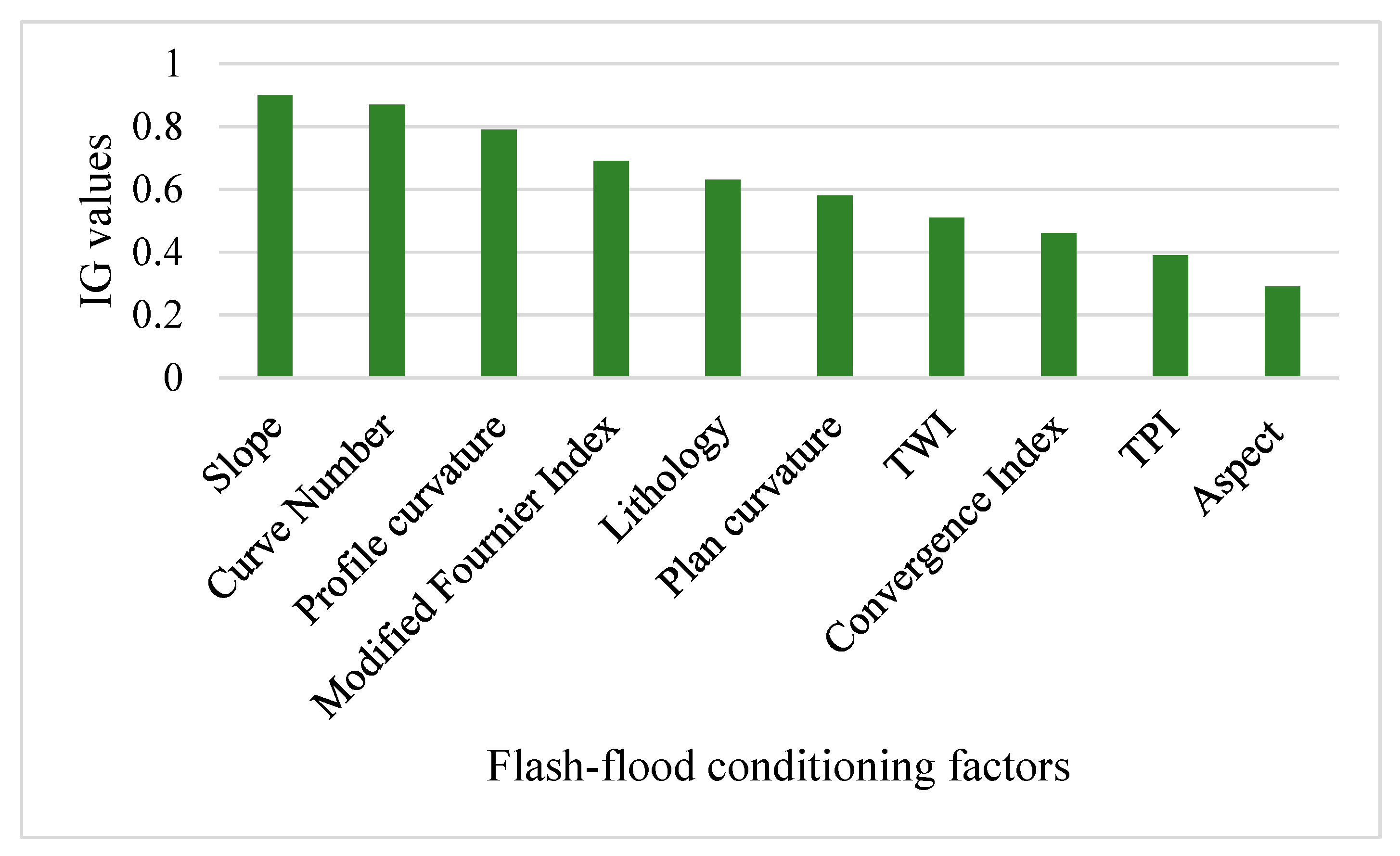
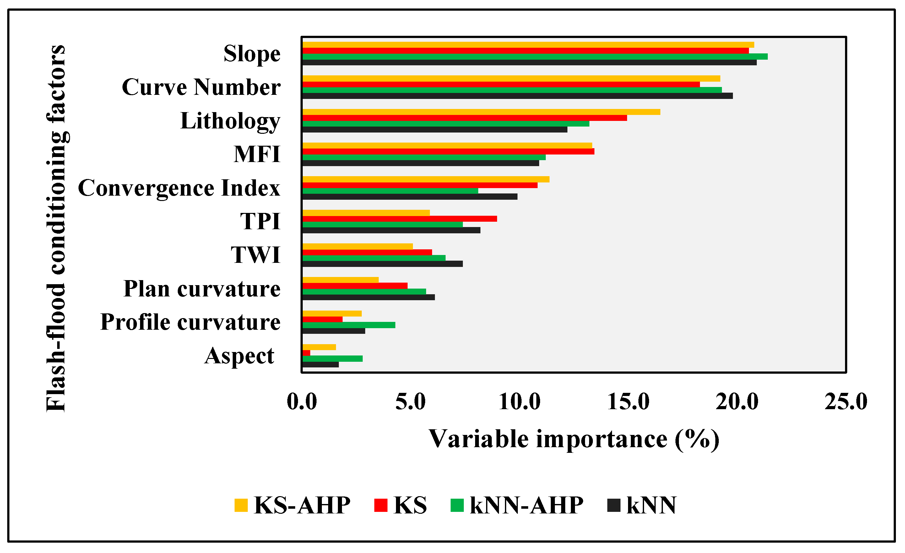
6.1. Predictive Ability of Flash-Flood Conditioning Factors
6.2. AHP Weights Results
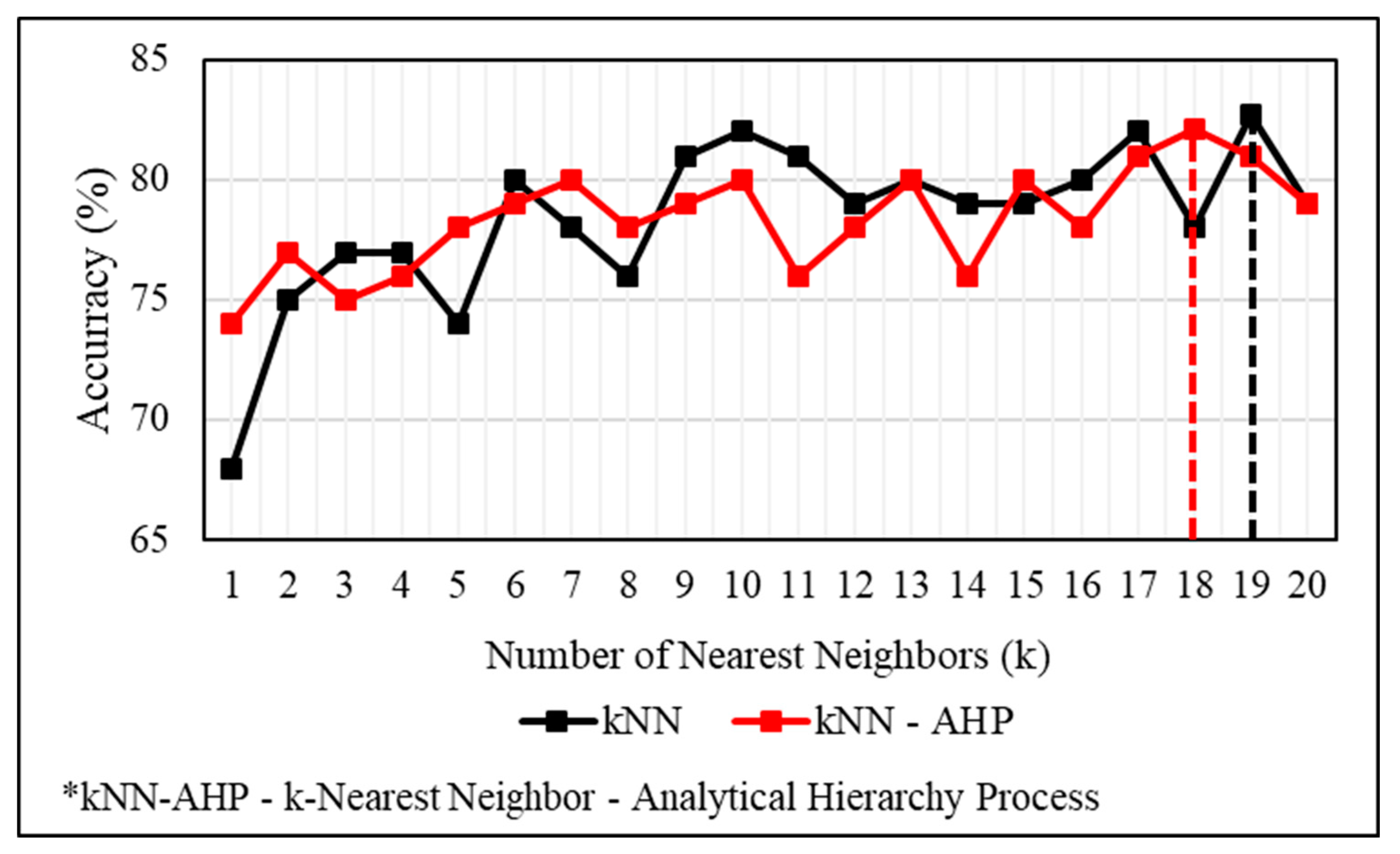
6.3. Application of kNN and kNN–AHP Ensemble Model
6.4. Application of KS and KS–AHP Ensemble Model
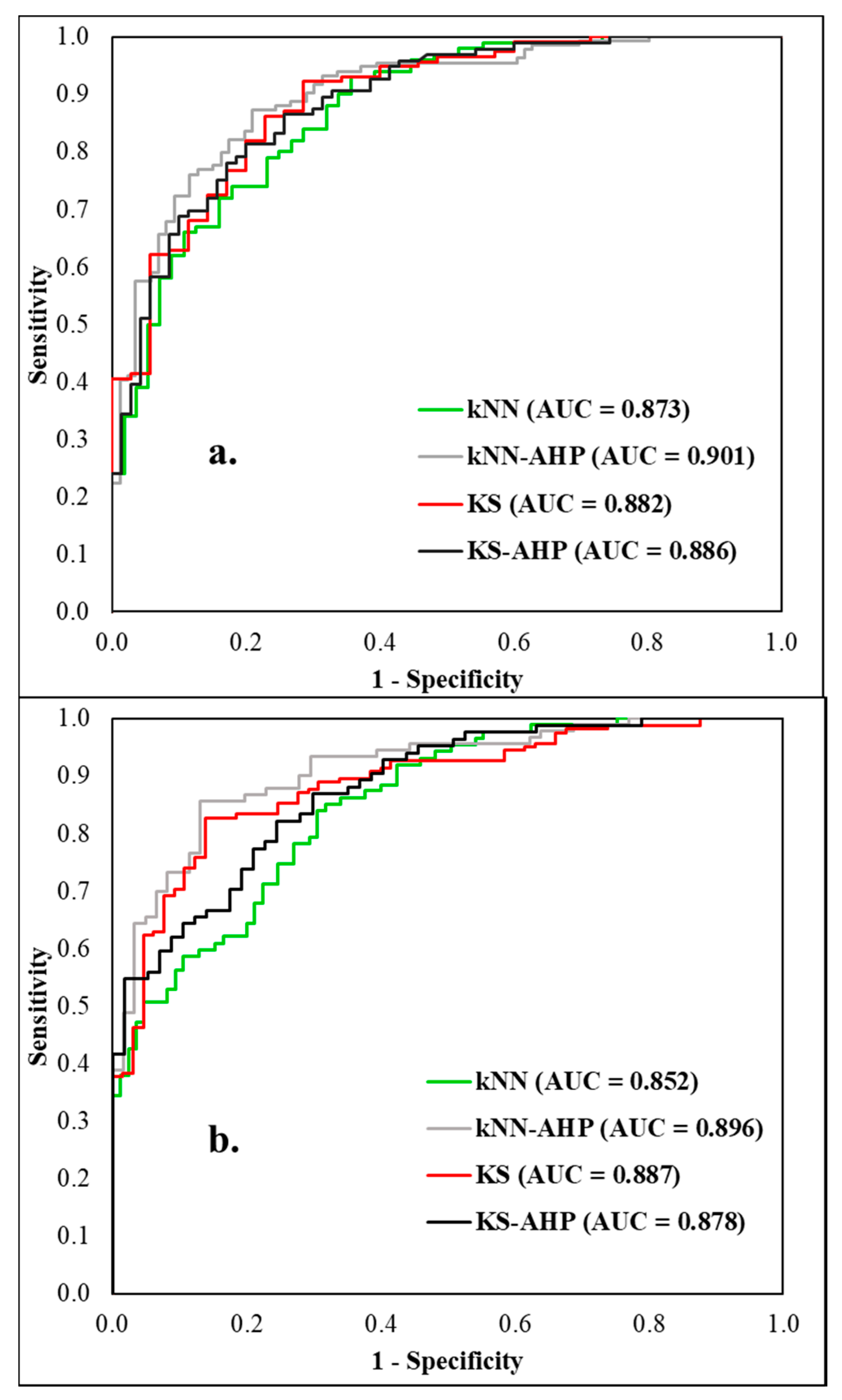
6.5. Results Validation
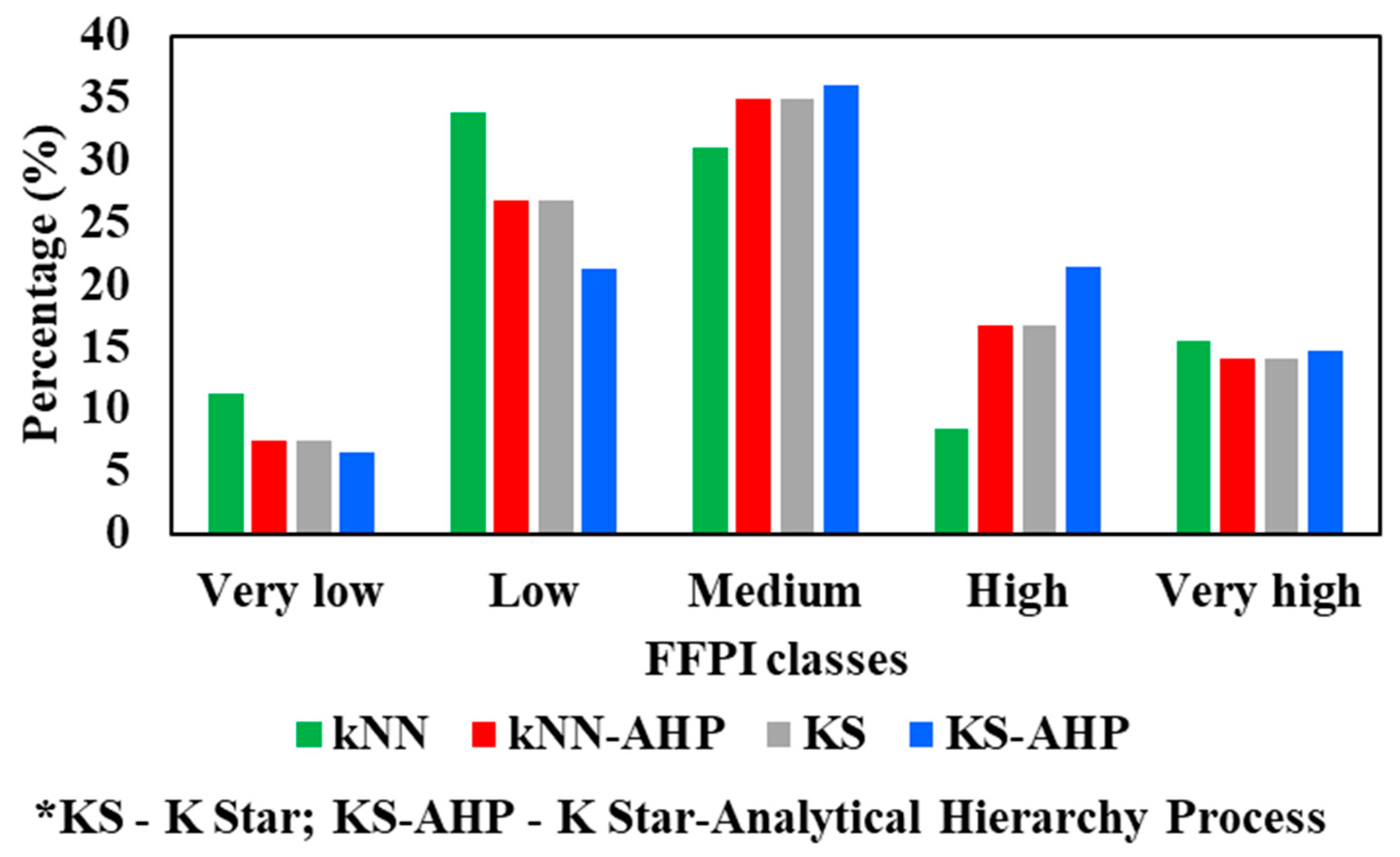
6.5.1. Share of Torrential Pixels in FFPI Classes
6.5.2. Receiver Operating Characteristic (ROC) Curve
7. Conclusions
Supplementary Materials
Author Contributions
Funding
Acknowledgments
Conflicts of Interest
References
- Costache, R. Flood Susceptibility Assessment by Using Bivariate Statistics and Machine Learning Models-A Useful Tool for Flood Risk Management. Water Resour. Manag. 2019, 33, 3239–3256. [Google Scholar] [CrossRef]
- Termeh, S.V.R.; Kornejady, A.; Pourghasemi, H.R.; Keesstra, S. Flood susceptibility mapping using novel ensembles of adaptive neuro fuzzy inference system and metaheuristic algorithms. Sci. Total Environ. 2018, 615, 438–451. [Google Scholar] [CrossRef] [PubMed]
- Hong, H.; Tsangaratos, P.; Ilia, I.; Liu, J.; Zhu, A.-X.; Chen, W. Application of fuzzy weight of evidence and data mining techniques in construction of flood susceptibility map of Poyang County, China. Sci. Total Environ. 2018, 625, 575–588. [Google Scholar] [CrossRef] [PubMed]
- Costache, R. Flash-Flood Potential assessment in the upper and middle sector of Prahova river catchment (Romania). A comparative approach between four hybrid models. Sci. Total Environ. 2019, 659, 1115–1134. [Google Scholar] [CrossRef]
- Elkhrachy, I. Flash flood hazard mapping using satellite images and GIS tools: A case study of Najran City, Kingdom of Saudi Arabia (KSA). Egypt. J. Remote Sens. Space Sci. 2015, 18, 261–278. [Google Scholar] [CrossRef] [Green Version]
- Jacinto, R.; Grosso, N.; Reis, E.; Dias, L.; Santos, F.; Garrett, P. Continental Portuguese Territory Flood Susceptibility Index: Contribution to a vulnerability index. Nat. Hazards Earth Syst. Sci. 2015, 15, 1907–1919. [Google Scholar] [CrossRef] [Green Version]
- Khosravi, K.; Pham, B.T.; Chapi, K.; Shirzadi, A.; Shahabi, H.; Revhaug, I.; Prakash, I.; Bui, D.T. A comparative assessment of decision trees algorithms for flash flood susceptibility modeling at Haraz watershed, northern Iran. Sci. Total Environ. 2018, 627, 744–755. [Google Scholar] [CrossRef]
- Youssef, A.M.; Pradhan, B.; Sefry, S.A. Flash flood susceptibility assessment in Jeddah city (Kingdom of Saudi Arabia) using bivariate and multivariate statistical models. Environ. Earth Sci. 2016, 75, 12. [Google Scholar] [CrossRef]
- Norbiato, D.; Borga, M.; Degli Esposti, S.; Gaume, E.; Anquetin, S. Flash flood warning based on rainfall thresholds and soil moisture conditions: An assessment for gauged and ungauged basins. J. Hydrol. 2008, 362, 274–290. [Google Scholar] [CrossRef]
- Georgakakos, K.P. Modern operational flash flood warning systems based on flash flood guidance theory: Performance evaluation. In Proceedings of the International Conference on Innovation Advances and Implementation of Flood Forecasting Technology, Bergen-Tromsø, Norway, 9–13 October 2005; pp. 9–13. [Google Scholar]
- Sweeney, T.L. Modernized Areal Flash Flood Guidance; NOAA Technical Memorandum NWS HYDRO 44; Hydrology Laboratory, National Weather Service, NOAA: Silver Spring, MD, USA, 1992; pp. 1–21. [Google Scholar]
- Carpenter, T.; Sperfslage, J.; Georgakakos, K.; Sweeney, T.; Fread, D. National threshold runoff estimation utilizing GIS in support of operational flash flood warning systems. J. Hydrol. 1999, 224, 21–44. [Google Scholar] [CrossRef]
- Georgakakos, K.P. Analytical results for operational flash flood guidance. J. Hydrol. 2006, 317, 81–103. [Google Scholar] [CrossRef]
- Ntelekos, A.A.; Georgakakos, K.P.; Krajewski, W.F. On the uncertainties of flash flood guidance: Toward probabilistic forecasting of flash floods. J. Hydrometeorol. 2006, 7, 896–915. [Google Scholar] [CrossRef]
- Petroselli, A.; Vojtek, M.; Vojteková, J. Flood mapping in small ungauged basins: A comparison of different approaches for two case studies in Slovakia. Hydrol. Res. 2019, 50, 379–392. [Google Scholar] [CrossRef] [Green Version]
- Costache, R.; Bui, D.T. Spatial prediction of flood potential using new ensembles of bivariate statistics and artificial intelligence: A case study at the Putna river catchment of Romania. Sci. Total Environ. 2019, 691, 1098–1118. [Google Scholar] [CrossRef]
- Bui, D.T.; Hoang, N.-D.; Martínez-Álvarez, F.; Ngo, P.-T.T.; Hoa, P.V.; Pham, T.D.; Samui, P.; Costache, R. A novel deep learning neural network approach for predicting flash flood susceptibility: A case study at a high frequency tropical storm area. Sci. Total Environ. 2020, 701, 134413. [Google Scholar]
- Zhao, G.; Pang, B.; Xu, Z.; Yue, J.; Tu, T. Mapping flood susceptibility in mountainous areas on a national scale in China. Sci. Total Environ. 2018, 615, 1133–1142. [Google Scholar] [CrossRef]
- Mohammady, M.; Pourghasemi, H.R.; Amiri, M. Assessment of land subsidence susceptibility in Semnan plain (Iran): A comparison of support vector machine and weights of evidence data mining algorithms. Nat. Hazards 2019, 99, 951–971. [Google Scholar] [CrossRef]
- Tehrany, M.S.; Pradhan, B.; Jebur, M.N. Flood susceptibility mapping using a novel ensemble weights-of-evidence and support vector machine models in GIS. J. Hydrol. 2014, 512, 332–343. [Google Scholar] [CrossRef]
- Tehrany, M.S.; Kumar, L. The application of a Dempster–Shafer-based evidential belief function in flood susceptibility mapping and comparison with frequency ratio and logistic regression methods. Environ. Earth Sci. 2018, 77, 490. [Google Scholar] [CrossRef]
- Shafapour Tehrany, M.; Kumar, L.; Neamah Jebur, M.; Shabani, F. Evaluating the application of the statistical index method in flood susceptibility mapping and its comparison with frequency ratio and logistic regression methods. Geomat. Nat. Hazards Risk 2019, 10, 79–101. [Google Scholar] [CrossRef]
- Rahmati, O.; Pourghasemi, H.R.; Zeinivand, H. Flood susceptibility mapping using frequency ratio and weights-of-evidence models in the Golastan Province, Iran. Geocarto Int. 2016, 31, 42–70. [Google Scholar] [CrossRef]
- Khosravi, K.; Pourghasemi, H.R.; Chapi, K.; Bahri, M. Flash flood susceptibility analysis and its mapping using different bivariate models in Iran: A comparison between Shannon’s entropy, statistical index, and weighting factor models. Environ. Monit. Assess. 2016, 188, 656. [Google Scholar] [CrossRef] [PubMed]
- Azareh, A.; Rahmati, O.; Rafiei-Sardooi, E.; Sankey, J.B.; Lee, S.; Shahabi, H.; Ahmad, B.B. Modelling gully-erosion susceptibility in a semi-arid region, Iran: Investigation of applicability of certainty factor and maximum entropy models. Sci. Total Environ. 2019, 655, 684–696. [Google Scholar] [CrossRef] [PubMed]
- Souissi, D.; Zouhri, L.; Hammami, S.; Msaddek, M.H.; Zghibi, A.; Dlala, M. GIS-based MCDM-AHP modeling for flood susceptibility mapping of arid areas, southeastern Tunisia. Geocarto Int. 2019, 1–25. [Google Scholar] [CrossRef]
- Khosravi, K.; Shahabi, H.; Pham, B.T.; Adamowski, J.; Shirzadi, A.; Pradhan, B.; Dou, J.; Ly, H.-B.; Gróf, G.; Ho, H.L. A comparative assessment of flood susceptibility modeling using Multi-Criteria Decision-Making Analysis and Machine Learning Methods. J. Hydrol. 2019, 573, 311–323. [Google Scholar] [CrossRef]
- Kim, T.H.; Kim, B.; Han, K.-Y. Application of Fuzzy TOPSIS to Flood Hazard Mapping for Levee Failure. Water 2019, 11, 592. [Google Scholar] [CrossRef] [Green Version]
- Shafizadeh-Moghadam, H.; Valavi, R.; Shahabi, H.; Chapi, K.; Shirzadi, A. Novel forecasting approaches using combination of machine learning and statistical models for flood susceptibility mapping. J. Environ. Manag. 2018, 217, 1–11. [Google Scholar] [CrossRef] [Green Version]
- Pham, Q.B.; Abba, S.I.; Usman, A.G.; Linh, N.T.T.; Gupta, V.; Malik, A.; Costache, R.; Vo, N.D.; Tri, D.Q. Potential of Hybrid Data-Intelligence Algorithms for Multi-Station Modelling of Rainfall. Water Resour. Manag. 2019, 1–21. [Google Scholar] [CrossRef]
- Choubin, B.; Moradi, E.; Golshan, M.; Adamowski, J.; Sajedi-Hosseini, F.; Mosavi, A. An Ensemble prediction of flood susceptibility using multivariate discriminant analysis, classification and regression trees, and support vector machines. Sci. Total Environ. 2019, 651, 2087–2096. [Google Scholar] [CrossRef]
- Tehrany, M.S.; Pradhan, B.; Jebur, M.N. Flood susceptibility analysis and its verification using a novel ensemble support vector machine and frequency ratio method. Stoch. Environ. Res. Risk Assess. 2015, 29, 1149–1165. [Google Scholar] [CrossRef]
- Ahmadlou, M.; Karimi, M.; Alizadeh, S.; Shirzadi, A.; Parvinnejhad, D.; Shahabi, H.; Panahi, M. Flood susceptibility assessment using integration of adaptive network-based fuzzy inference system (ANFIS) and biogeography-based optimization (BBO) and BAT algorithms (BA). Geocarto Int. 2019, 34, 1252–1272. [Google Scholar] [CrossRef]
- Bui, D.T.; Ngo, P.-T.T.; Pham, T.D.; Jaafari, A.; Minh, N.Q.; Hoa, P.V.; Samui, P. A novel hybrid approach based on a swarm intelligence optimized extreme learning machine for flash flood susceptibility mapping. Catena 2019, 179, 184–196. [Google Scholar] [CrossRef]
- Tien Bui, D.; Khosravi, K.; Shahabi, H.; Daggupati, P.; Adamowski, J.F.; Melesse, A.M.; Thai Pham, B.; Pourghasemi, H.R.; Mahmoudi, M.; Bahrami, S. Flood spatial modeling in northern Iran using remote sensing and gis: A comparison between evidential belief functions and its ensemble with a multivariate logistic regression model. Remote Sens. 2019, 11, 1589. [Google Scholar] [CrossRef] [Green Version]
- Wang, Y.; Hong, H.; Chen, W.; Li, S.; Pamučar, D.; Gigović, L.; Drobnjak, S.; Bui, D.T.; Duan, H. A hybrid GIS multi-criteria decision-making method for flood susceptibility mapping at Shangyou, China. Remote Sens. 2019, 11, 62. [Google Scholar] [CrossRef] [Green Version]
- Costache, R. Flash-flood Potential Index mapping using weights of evidence, decision Trees models and their novel hybrid integration. Stoch. Environ. Res. Risk Assess. 2019, 33, 1375–1402. [Google Scholar] [CrossRef]
- Costache, R.; Zaharia, L. Flash-flood potential assessment and mapping by integrating the weights-of-evidence and frequency ratio statistical methods in GIS environment–case study: Bâsca Chiojdului River catchment (Romania). J. Earth Syst. Sci. 2017, 126, 59. [Google Scholar] [CrossRef]
- Farr, T.G.; Rosen, P.A.; Caro, E.; Crippen, R.; Duren, R.; Hensley, S.; Kobrick, M.; Paller, M.; Rodriguez, E.; Roth, L. The shuttle radar topography mission. Rev. Geophys. 2007, 45, 1–33. [Google Scholar] [CrossRef] [Green Version]
- Van Zyl, J.J. The Shuttle Radar Topography Mission (SRTM): A breakthrough in remote sensing of topography. Acta Astronaut. 2001, 48, 559–565. [Google Scholar] [CrossRef]
- Costache, R.; Fontanine, I.; Corodescu, E. Assessment of surface runoff depth changes in Sǎrǎţel River basin, Romania using GIS techniques. Open Geosci. 2014, 6, 363–372. [Google Scholar]
- Costache, R.; Pravalie, R.; Mitof, I.; Popescu, C. Flood vulnerability assessment in the low sector of Saratel Catchment. Case study: Joseni Village. Carpathian J. Earth Environ. Sci. 2015, 10, 161–169. [Google Scholar]
- Zaharia, L.; Costache, R.; Prăvălie, R.; Ioana-Toroimac, G. Mapping flood and flooding potential indices: A methodological approach to identifying areas susceptible to flood and flooding risk. Case study: The Prahova catchment (Romania). Front. Earth Sci. 2017, 11, 229–247. [Google Scholar] [CrossRef]
- Shehata, M.; Mizunaga, H. Geospatial analysis of surface hydrological parameters for Kyushu Island, Japan. Nat. Hazards 2019, 96, 33–52. [Google Scholar] [CrossRef]
- Costache, R. Using GIS techniques for assessing lag time and concentration time in small river basins. Case study: Pecineaga river basin, Romania. Geogr. Tech. 2014, 9, 31–38. [Google Scholar]
- COSTACHE, R. Estimating multiannual average runoff depth in the middle and upper sectors of Buzău River Basin. Geogr. Tech. 2014, 9, 21–29. [Google Scholar]
- Prăvălie, R.; Costache, R. The vulnerability of the territorial-administrative units to the hydrological phenomena of risk (flash-floods). Case study: The subcarpathian sector of Buzău catchment. Analele Univ. Din Oradea–Seria Geogr. 2013, 23, 91–98. [Google Scholar]
- Pravalie, R.; Costache, R. The Analysis of the Susceptibility of the Flash-Floods’ Genesis in the Area of the Hydrographical Basin of Bāsca Chiojdului River/Analiza susceptibilitatii Genezei Viiturilor īn Aria Bazinului Hidrografic al Rāului Bāsca Chiojdului; Department of Geography, University of Craiova: Craiova, Romania, 2014; Volume 13, p. 39. [Google Scholar]
- Zaharia, L.; Costache, R.; Prăvălie, R.; Minea, G. Assessment and mapping of flood potential in the Slănic catchment in Romania. J. Earth Syst. Sci. 2015, 124, 1311–1324. [Google Scholar] [CrossRef] [Green Version]
- Kourgialas, N.N.; Karatzas, G.P. Flood management and a GIS modelling method to assess flood-hazard areas—A case study. Hydrol. Sci. J. J. Sci. Hydrol. 2011, 56, 212–225. [Google Scholar] [CrossRef]
- Corrao, M.V.; Link, T.E.; Heinse, R.; Eitel, J.U. Modeling of terracette-hillslope soil moisture as a function of aspect, slope and vegetation in a semi-arid environment. Earth Surf. Process. Landf. 2017, 42, 1560–1572. [Google Scholar] [CrossRef]
- Dahri, N.; Abida, H. Monte Carlo simulation-aided analytical hierarchy process (AHP) for flood susceptibility mapping in Gabes Basin (southeastern Tunisia). Environ. Earth Sci. 2017, 76, 302. [Google Scholar] [CrossRef]
- Minea, G. Assessment of the flash flood potential of Bâsca River Catchment (Romania) based on physiographic factors. Open Geosci. 2013, 5, 344–353. [Google Scholar] [CrossRef] [Green Version]
- Pradhan, B.; Lee, S. Delineation of landslide hazard areas on Penang Island, Malaysia, by using frequency ratio, logistic regression, and artificial neural network models. Environ. Earth Sci. 2010, 60, 1037–1054. [Google Scholar] [CrossRef]
- Martina, M.L.; Entekhabi, D. Identification of runoff generation spatial distribution using conventional hydrologic gauge time series. Water Resour. Res. 2006, 42, 1–9. [Google Scholar] [CrossRef]
- Costache, R.; Prăvălie, R. The analysis of May 29 2012 flood phenomena in the lower sector of Slănic drainage basin (case of Cernăteşti locality area). GEOREVIEW Sci. Ann. Stefan Cel Mare Univ. Suceava Geogr. Ser. 2013, 22, 78–87. [Google Scholar] [CrossRef] [Green Version]
- Jenness, J.S. The Effects of Fire on Mexican Spotted Owls in Arizona and New Mexico. Master’s Thesis, Northern Arizona University, Flagstaff, AZ, USA, 2000. [Google Scholar]
- Kirkby, M.; Beven, K. A physically based, variable contributing area model of basin hydrology. Hydrol. Sci. J. 1979, 24, 43–69. [Google Scholar]
- Saaty, T.L. The Analytical Hierarchy Process, Planning, Priority Setting, Resource Allocation (Decision Making Series); McGraw-Hill: New York, NY, USA, 1980. [Google Scholar]
- Shahabi, H.; Khezri, S.; Ahmad, B.B.; Hashim, M. Landslide susceptibility mapping at central Zab basin, Iran: A comparison between analytical hierarchy process, frequency ratio and logistic regression models. Catena 2014, 115, 55–70. [Google Scholar] [CrossRef]
- Chen, W.; Li, W.; Chai, H.; Hou, E.; Li, X.; Ding, X. GIS-based landslide susceptibility mapping using analytical hierarchy process (AHP) and certainty factor (CF) models for the Baozhong region of Baoji City, China. Environ. Earth Sci. 2016, 75, 63. [Google Scholar] [CrossRef]
- Ghosh, A.; Kar, S.K. Application of analytical hierarchy process (AHP) for flood risk assessment: A case study in Malda district of West Bengal, India. Nat. Hazards 2018, 94, 349–368. [Google Scholar] [CrossRef]
- Razandi, Y.; Pourghasemi, H.R.; Neisani, N.S.; Rahmati, O. Application of analytical hierarchy process, frequency ratio, and certainty factor models for groundwater potential mapping using GIS. Earth Sci. Inform. 2015, 8, 867–883. [Google Scholar] [CrossRef]
- Saaty, T.L. A scaling method for priorities in hierarchical structures. J. Math. Psychol. 1977, 15, 234–281. [Google Scholar] [CrossRef]
- Kumar, R.; Anbalagan, R. Landslide susceptibility mapping using analytical hierarchy process (AHP) in Tehri reservoir rim region, Uttarakhand. J. Geol. Soc. India 2016, 87, 271–286. [Google Scholar] [CrossRef]
- Marjanovic, M.; Bajat, B.; Kovacevic, M. Landslide susceptibility assessment with machine learning algorithms. In Proceedings of the IEEE International Conference on Intelligent. Networking and Collaborative Systems, Barcelona, Spain, 4–6 November 2009; pp. 273–278. [Google Scholar]
- Arefin, A.S.; Riveros, C.; Berretta, R.; Moscato, P. Gpu-fs-knn: A software tool for fast and scalable knn computation using gpus. PLoS ONE 2012, 7, e44000. [Google Scholar] [CrossRef] [PubMed] [Green Version]
- Sabokbar, H.F.; Roodposhti, M.S.; Tazik, E. Landslide susceptibility mapping using geographically-weighted principal component analysis. Geomorphology 2014, 226, 15–24. [Google Scholar] [CrossRef]
- James, G.; Witten, D.; Hastie, T.; Tibshirani, R. An Introduction to Statistical Learning; Springer: New York, NY, USA, 2013; Volume 112. [Google Scholar]
- Thirumuruganathan, S. A detailed introduction to K-nearest neighbor (KNN) algorithm. Retrieved March 2010, 20, 2012. [Google Scholar]
- Kavzoglu, T.; Colkesen, I. Entropic distance based K-Star algorithm for remote sensing image classification. Fresenius Environ. Bull. 2011, 20, 1200–1207. [Google Scholar]
- Morrison, D.; De Silva, L.C. Voting ensembles for spoken affect classification. J. Netw. Comput. Appl. 2007, 30, 1356–1365. [Google Scholar] [CrossRef]
- Cleary, J.G.; Trigg, L.E. K*: An instance-based learner using an entropic distance measure. In Machine Learning Proceedings 1995; Elsevier: Amsterdam, The Netherlands, 1995; pp. 108–114. [Google Scholar]
- Sharma, R.; Kumar, S.; Maheshwari, R. Comparative analysis of classification techniques in data mining using different datasets. Int. J. Comput. Sci. Mob. Comput. 2015, 4, 125–134. [Google Scholar]
- Bouckaert, R.R.; Frank, E.; Hall, M.; Kirkby, R.; Reutemann, P.; Seewald, A.; Scuse, D. Weka Manual for Version 3-6-0; University of Waikato: Hamilton, New Zealand, 2008; pp. 1–341. [Google Scholar]
- Chapi, K.; Singh, V.P.; Shirzadi, A.; Shahabi, H.; Bui, D.T.; Pham, B.T.; Khosravi, K. A novel hybrid artificial intelligence approach for flood susceptibility assessment. Environ. Model. Softw. 2017, 95, 229–245. [Google Scholar] [CrossRef]
- Tien Bui, D.; Shahabi, H.; Shirzadi, A.; Chapi, K.; Hoang, N.-D.; Pham, B.; Bui, Q.-T.; Tran, C.-T.; Panahi, M.; Bin Ahamd, B. A novel integrated approach of relevance vector machine optimized by imperialist competitive algorithm for spatial modeling of shallow landslides. Remote Sens. 2018, 10, 1538. [Google Scholar] [CrossRef] [Green Version]
- Costache, R.; Hong, H.; Wang, Y. Identification of torrential valleys using GIS and a novel hybrid integration of artificial intelligence, machine learning and bivariate statistics. Catena 2019, 183, 104179. [Google Scholar] [CrossRef]
- Park, S.-J.; Lee, C.-W.; Lee, S.; Lee, M.-J. Landslide susceptibility mapping and comparison using decision tree models: A Case Study of Jumunjin Area, Korea. Remote Sens. 2018, 10, 1545. [Google Scholar] [CrossRef] [Green Version]
- Wang, Y.; Hong, H.; Chen, W.; Li, S.; Panahi, M.; Khosravi, K.; Shirzadi, A.; Shahabi, H.; Panahi, S.; Costache, R. Flood susceptibility mapping in Dingnan County (China) using adaptive neuro-fuzzy inference system with biogeography based optimization and imperialistic competitive algorithm. J. Environ. Manag. 2019, 247, 712–729. [Google Scholar] [CrossRef] [PubMed]
- Zhang, S. Nearest neighbor selection for iteratively kNN imputation. J. Syst. Softw. 2012, 85, 2541–2552. [Google Scholar] [CrossRef]
- Amiri, M.; Amnieh, H.B.; Hasanipanah, M.; Khanli, L.M. A new combination of artificial neural network and K-nearest neighbors models to predict blast-induced ground vibration and air-overpressure. Eng. Comput. 2016, 32, 631–644. [Google Scholar] [CrossRef]
- Nguyen, Q.-K.; Tien Bui, D.; Hoang, N.-D.; Trinh, P.; Nguyen, V.-H.; Yilmaz, I. A novel hybrid approach based on instance based learning classifier and rotation forest ensemble for spatial prediction of rainfall-induced shallow landslides using GIS. Sustainability 2017, 9, 813. [Google Scholar] [CrossRef] [Green Version]
- Naji, H.I.; Ali, R.H.; Al-Zubaidi, E.A. Risk Management Techniques. In Strategic Management-a Dynamic View; IntechOpen: London, UK, 2019. [Google Scholar]
- Chen, W.; Peng, J.; Hong, H.; Shahabi, H.; Pradhan, B.; Liu, J.; Zhu, A.-X.; Pei, X.; Duan, Z. Landslide susceptibility modelling using GIS-based machine learning techniques for Chongren County, Jiangxi Province, China. Sci. Total Environ. 2018, 626, 1121–1135. [Google Scholar] [CrossRef]
- Alizadeh, M.; Ngah, I.; Hashim, M.; Pradhan, B.; Pour, A. A hybrid analytic network process and artificial neural network (ANP-ANN) model for urban earthquake vulnerability assessment. Remote Sens. 2018, 10, 975. [Google Scholar] [CrossRef] [Green Version]
- Kadavi, P.; Lee, C.-W.; Lee, S. Application of ensemble-based machine learning models to landslide susceptibility mapping. Remote Sens. 2018, 10, 1252. [Google Scholar] [CrossRef] [Green Version]
- Djeddaoui, F.; Chadli, M.; Gloaguen, R. Desertification susceptibility mapping using logistic regression analysis in the Djelfa area, Algeria. Remote Sens. 2017, 9, 1031. [Google Scholar] [CrossRef] [Green Version]
- Chen, J.; Yang, S.; Li, H.; Zhang, B.; Lv, J. Research on geographical environment unit division based on the method of natural breaks (Jenks). Int. Arch. Photogramm. Remote Sens. Spat. Inf. Sci. 2013, XL-4/W3, 47–50. [Google Scholar] [CrossRef] [Green Version]
- Bui, D.T.; Nguyen, Q.P.; Hoang, N.-D.; Klempe, H. A novel fuzzy K-nearest neighbor inference model with differential evolution for spatial prediction of rainfall-induced shallow landslides in a tropical hilly area using GIS. Landslides 2017, 14, 1–17. [Google Scholar]
- General Inspectorate for Emergency Situation. The Archive of General Inspectorate for Emergency Situation-Prahova County Subsidiary, Romania; General Inspectorate for Emergency Situation: Bucharest, Romania, November 2019. [Google Scholar]


| Factors | N | λmax | CI | RI | CR |
|---|---|---|---|---|---|
| Slope angle | 5 | 5.196 | 0.049 | 1.12 | 0.040 |
| TPI | 5 | 5.029 | 0.007 | 1.12 | 0.010 |
| TWI | 5 | 5.058 | 0.014 | 1.12 | 0.010 |
| Curve Number | 6 | 6.105 | 0.021 | 1.24 | 0.017 |
| Lithology | 12 | 13.12 | 0.101 | 1.53 | 0.066 |
| Profile curvature | 3 | 3.039 | 0.019 | 0.58 | 0.030 |
| Plan curvature | 3 | 3.109 | 0.054 | 0.58 | 0.090 |
| Slope aspect | 9 | 9.200 | 0.025 | 1.45 | 0.020 |
| Convergence index | 5 | 5.099 | 0.025 | 1.12 | 0.020 |
| Modified Fournier Index | 5 | 5.043 | 0.011 | 1.12 | 0.010 |
| Models | Sample | True Positive | True Negative | False Positive | False Negative | Sensitivity | Specificity | Accuracy |
|---|---|---|---|---|---|---|---|---|
| kNN | Training | 172,362 | 147,766 | 25,271 | 41,875 | 0.805 | 0.854 | 0.827 |
| Validating | 71,373 | 72,943 | 13,750 | 18,917 | 0.790 | 0.841 | 0.815 | |
| kNN–AHP | Training | 166,392 | 149,694 | 26,407 | 42,468 | 0.797 | 0.850 | 0.821 |
| Validating | 63,203 | 63,920 | 14,862 | 15,299 | 0.805 | 0.811 | 0.808 | |
| KS | Training | 154,893 | 149,026 | 30,764 | 43,678 | 0.780 | 0.829 | 0.803 |
| Validating | 63,402 | 53,218 | 14,313 | 11,604 | 0.845 | 0.788 | 0.818 | |
| KS–AHP | Training | 152,754 | 142,657 | 25,547 | 40,419 | 0.791 | 0.848 | 0.817 |
| Validating | 52,347 | 51,934 | 18,012 | 5589 | 0.904 | 0.742 | 0.815 |
| FFPI Class | Training Areas | Validating Areas | ||||||
|---|---|---|---|---|---|---|---|---|
| kNN | kNN–AHP | KS | KS–AHP | kNN | kNN–AHP | KS | KS–AHP | |
| Very low | 1.43% | 2.5% | 1.57% | 2.56% | 5.43% | 4.21% | 3.95% | 4.8% |
| Low | 5.67% | 4.32% | 3.88% | 7.44% | 7.43% | 5.12% | 6.43% | 6.89% |
| Medium | 13.45% | 7.43% | 10.34% | 8.65% | 12.24% | 10.93% | 14.39% | 11.32% |
| High | 27.52% | 31.43% | 35.43% | 25.73% | 32.45% | 31.73% | 29.54% | 33.45% |
| Very high | 51.93% | 54.32% | 48.78% | 55.62% | 42.45% | 48.01% | 45.69% | 43.54% |
© 2019 by the authors. Licensee MDPI, Basel, Switzerland. This article is an open access article distributed under the terms and conditions of the Creative Commons Attribution (CC BY) license (http://creativecommons.org/licenses/by/4.0/).
Share and Cite
Costache, R.; Pham, Q.B.; Sharifi, E.; Linh, N.T.T.; Abba, S.I.; Vojtek, M.; Vojteková, J.; Nhi, P.T.T.; Khoi, D.N. Flash-Flood Susceptibility Assessment Using Multi-Criteria Decision Making and Machine Learning Supported by Remote Sensing and GIS Techniques. Remote Sens. 2020, 12, 106. https://0-doi-org.brum.beds.ac.uk/10.3390/rs12010106
Costache R, Pham QB, Sharifi E, Linh NTT, Abba SI, Vojtek M, Vojteková J, Nhi PTT, Khoi DN. Flash-Flood Susceptibility Assessment Using Multi-Criteria Decision Making and Machine Learning Supported by Remote Sensing and GIS Techniques. Remote Sensing. 2020; 12(1):106. https://0-doi-org.brum.beds.ac.uk/10.3390/rs12010106
Chicago/Turabian StyleCostache, Romulus, Quoc Bao Pham, Ehsan Sharifi, Nguyen Thi Thuy Linh, S.I. Abba, Matej Vojtek, Jana Vojteková, Pham Thi Thao Nhi, and Dao Nguyen Khoi. 2020. "Flash-Flood Susceptibility Assessment Using Multi-Criteria Decision Making and Machine Learning Supported by Remote Sensing and GIS Techniques" Remote Sensing 12, no. 1: 106. https://0-doi-org.brum.beds.ac.uk/10.3390/rs12010106