A Method for the Optimized Design of a Rain Gauge Network Combined with Satellite Remote Sensing Data


1
Department of Water Resources, China Institute of Water Resources and Hydropower Research, Beijing 100038, China
2
State Key Laboratory of Simulation and Regulation of Water Cycle in River Basin, China Institute of Water Resources and Hydropower Research, Beijing 100038, China
3
Sichuan Academy of Water Conservancy, Chengdu 610000, China
*
Author to whom correspondence should be addressed.
Remote Sens. 2020, 12(1), 194; https://0-doi-org.brum.beds.ac.uk/10.3390/rs12010194
Submission received: 25 November 2019
/
Revised: 30 December 2019
/
Accepted: 3 January 2020
/
Published: 5 January 2020
(This article belongs to the Section Remote Sensing in Geology, Geomorphology and Hydrology)
Abstract
:A well-designed rain gauge network can provide precise and detailed rainfall data for earth science research; meanwhile, satellite precipitation data has been developed to generate more real spatial features, which provides new data support for the improvement of ground station network design methods. In this paper, satellite precipitation data are introduced into the design of a rain gauge network and an optimized method for designing a rain gauge network that comprehensively considers the information content, spatiotemporality, and accuracy (ISA) of the data is proposed. After screening the potential stations, the average spatial information index of the rain gauge network, which is calculated from remote sensing data, is used to address the shortcomings of applying spatial information from single-use measurement data. Then, the greedy ranking algorithm is used to rank the order in which the rain gauges are added to the network. The results of the rain gauge network design in the upper reaches of the Chaobai river show that compared with two methods that do not consider spatiality or use only measured data to consider spatiality, the proposed method performs better in terms of the spatial layout and accuracy verification. This study provides new ideas and references for the design of hydrological station networks and explores the use of remote sensing data for the layout of ground-based station networks.
1. Introduction
Ground-based observations of precipitation are the most basic data in hydrology and provide fundamental information for Earth sciences. Rain gauge networks are very important for water resource planning, management, development, and utilization. One of the key issues in hydrological measurements is to improve the scientific rationality and optimization of rain gauge network design in regions. In the design of a rain gauge network, although the World Meteorological Organization (WMO) has identified the minimum monitoring density requirements [1], unified methodological recommendations regarding the number and spatial locations of stations have been difficult to establish due to differences in topography, local climate, and meteorological conditions and local economic conditions. Generally, the networks of hydrological stations in many regions are arranged according to a grid, or ground stations are added according to the spatial distribution characteristics of ground stations based on regional interpolation data and funding conditions. The development of optical, active, and passive microwave remote sensing technology in recent years has provided a new and improved spatial data source for the layout of hydrological stations [2,3]. Therefore, it is meaningful and constructive to explore a network design method that acquires regional information more accurately with as few sites as possible in the new data environment.
Since the 1930s, quantitative research on the design of station networks has been conducted, and it can be classified according to the calculation methods into statistical methods, information entropy methods, expert knowledge methods, hybrid methods, and other methods [4,5]. Statistical methods, including the kriging interpolation, correlation coefficients, least squares, and other statistical methods, have been the most common methods used for network design for a long time because they utilize the minimum deviation as the design objective [6,7,8,9,10]. The method of expert knowledge develops a network design through experience and decision making (e.g., according to regional topographic characteristics, actual needs, and user surveys) [11,12]. The hybrid method applies the above two or more methods to design a station network [13,14,15]. In addition, according to the types of hydrological elements that are monitored, the station network design methods can be classified into a single hydrological element network design and multi-hydrological element network design [16].
The information entropy method is based on information theory [17], which was originally used to describe and evaluate the uncertainty of hydrological systems and models in hydrology [18]. This method has been gradually applied to the evaluation and design of optimized hydrological station networks by describing the change and exchange of information among hydrological stations [19,20,21]. The information entropy method maximizes the content of the information obtained by the network as the optimization objective by calculating the variable entropy, such as the minimum mutual information from the existing network [22,23], the maximum joint information and minimum mutual information [14,24,25,26,27], and the maximum information with minimum redundancy (MIMR) [28], which is widely used in station network design for different time periods and various hydrological elements [29,30]. In addition, a hybrid method that includes information entropy has been proposed. The optimization objective synthesizes the information content and other indicators for network design, such as the hydrological model accuracy [31], clustering characteristics [15], and interpolation accuracy [32], based on measurement data to ensure that the design of the station network is more comprehensive. However, because the calculation of optimization objectives is based on observation data from ground stations, this method is not guaranteed to capture the real and objective spatial distribution characteristics.
Compared with interpolation data or simulation data, remote sensing data have the advantage of objectively and comprehensively reflecting the spatial relationships of objects [33,34]. With the development of remote sensing technology, a series of precipitation inversion models and products have been developed. Satellite precipitation products and related downscaling precipitation products include TRMM (Tropic Rainfall Measurement Mission) [9], GPM (Global Precipitation Measurement) [35], CMOPRH (CPC MORPHing technique) [36], PERSIANN (Precipitation Estimation from Remotely Sensed Information using Artificial Neural Networks) [37], GPCP (Global Precipitation Climatology Project) [38], and PERSIANN-CCS (PERSIANN Cloud Classification System) [39]. Moreover, data fusion and data assimilation systems, such as CLDAS (CMA Land Data Assimilation System) [40] and GLDAS (Global Land Data Assimilation System) [41], also contain precipitation data. These satellite remote sensing products have nearly the same degree of temporal resolution as the measured data at the site, including hourly, daily, and lower temporal resolutions. Moreover, the spatial resolution ranges from 4 km to 25 km and coarser resolution. Satellite remote sensing products appear to be suitable for the design of rain gauge networks in order to generate better rainfall forecasts, flood range forecasts, and water cycle simulations. Attempts have been made to apply remote sensing data instead of measurement data or model simulation data for network layouts using information entropy and statistical methods [2,42,43]. However, because satellite remote sensing data may present problems with low resolution and uncertainty, relying solely on remote sensing data to evaluate the accuracy of a network is inappropriate [42]. In addition, compared with the remote sensing data of optical satellites, the numerical accuracy of radar data is improved to some extent. However, there are some difficulties in obtaining and retrieving radar data. Due to the limited amount of data, the spatiotemporal characteristics of a large range are not spatiotemporally continuous like local data; therefore, it is difficult to obtain a universal rainfall layout method. Although the combined application of remote sensing and ground observation data is undoubtedly beneficial to the optimization of station network layouts, only a few related studies have been performed. For example, Wang et al. [44] proposed a temporally continuous maximum coverage network layout method according to the ground-based measurements and space-borne rainfall sensors monitoring period using the maximal covering location problem model [45].
Compared with the data measured at rain gauges, satellite precipitation products have better spatial continuity, which can make identifying the location of rainfall sites more reasonable and effective. Local or global texture feature analyses of remote sensing data are widely used in image segmentation, object classification, and pattern recognition [46,47,48,49]. Among many texture analysis methods, the grayscale co-occurrence matrix (GLCM) method is the most common. For example, Li et al. built GLCM texture features using five characteristics, i.e., standard deviation, correlation, mean, contrast, and angular second moment, and then generating differential images at different moments via a combination of the spectra to monitor ground object changes in very-high-resolution remote sensing images [50].
As Chacon-Hurtado et al. [5] noted in their review, although nontraditional data sources obtained by various sensing technologies have the potential to complement traditional network design, new network design methods are needed to address heterogeneous dynamic data. This paper comprehensively applies the advantages of satellite precipitation data and ground station data to explore an optimal ground rainfall station network layout method with optimal comprehensive indicators of the information content, spatiotemporality, and accuracy (ISA). The paper is organized into five sections. The study area and data are introduced in the second section. The basic research methods, including information entropy theory, the kriging interpolation method, and the optimization layout method proposed in this paper, are introduced in the third section. The calculation results and discussion are presented in the fourth section, and the summary and prospect are provided in the fifth section.
2. Study Area and Data
2.1. Study Area
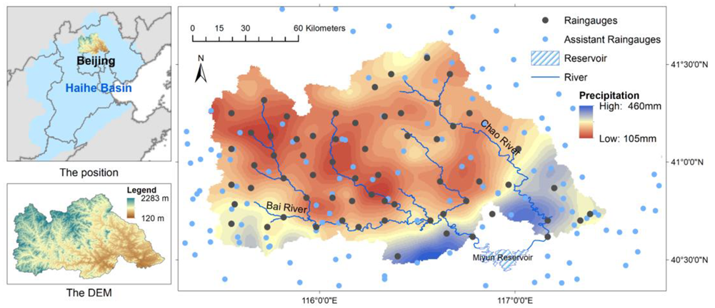
The Chaobai River is one of the main tributaries of the Haihe River Basin in China. The Chaobai River originates from the North China Plain, which has a semi-humid and semi-arid continental monsoon climate. The two tributaries of the Chaobai River, the Chao River and Bai River, converge into the Miyun Reservoir, which accounts for two-thirds of Beijing’s drinking water supply, from the northwest and southeast, respectively, and converge into the Chaobai River after discharge. This paper takes the upper reaches of the Chaobai River, that is, the basin above the Miyun Reservoir, as the research area. The study area covers an area of 136,000 km2, and it has an average annual precipitation value of 300–400 mm and average temperature of 9–10 °C. The precipitation from June to October accounts for more than 85% of the annual precipitation. The terrain is high in the northwest and low in the southeast, with an average elevation of 1010 m. The location and precipitation distribution of the study area of the average rainy season are shown in Figure 1.
2.2. Satellite Remote Sensing Data
PERSIANN-CCS is a satellite precipitation product that has high spatiotemporal resolution, with an hourly temporal resolution, a spatial resolution of 0.04° × 0.04°, and a coverage area of 60° N to 60° S [51]. This algorithm first extracts local and regional cloud features from longwave infrared geostationary satellite imagery (10.7 µm) and uses a neural network to relate the cloud classification and microwave data to estimate gridded rainfall. Detailed information is provided in [39,52,53]. Compared with other precipitation products, PERSIANN-CCS has the advantage of providing nearly real-time data at high spatial resolution. This product is widely used in flood warning and hydrological model simulations [54,55]. Nguyen et al. [56] reported that PERSIANN-CCS data could accurately capture the observed hydrograph shape via a simulation flood forecasting experiment, and the minimum correlation coefficient with real data reached 0.86. Zeweldi et al. [57] used radar rainfall observation data to evaluate the PERSIANN-CCS results and showed that the accuracy of PERSIANN-CCS can capture the patterns of intel-annual rainfall variability well. Cánovas-García et al. [58] evaluated three storm events and determined that the temporal distribution of rainfall was captured well by PERSIANN-CCS. Although Chang et al. [59] concluded that the absolute value of precipitation data from PERSIANN-CCS must be further improved, and many attempts to improve the accuracy of PERSIANN-CCS have been undertaken by the Center of Hydrometeorology and Remote Sensing at UCI (University of California, Irvine) [60,61], it is worth affirming that PERSIANN-CCS accurately reflects the spatial distribution characteristics of precipitation.
2.3. Data Preprocessing
Due to the inaccessibility of the observed rainfall data in 2014, the optimum design for the station network was determined using the observed data during June–October from 2006 to 2016 (excluding 2014) and remote sensing daily precipitation products from the same time. In this study, we randomly selected 25 stations as the initial network of the study area (544 km2/station) according to WMO minimum rainfall density standards (575 km2/station for hilly/undulating areas, 250 km2/station for mountainous areas) [1]. The interpolation results of the measured rain gauge data with sufficient density collected around the study area were taken as the true values to verify and evaluate the final results. The average number of stations for each interpolation is 80 (170 km2/station). Daily precipitation data can be provided consistently at 63 points in the study area, and discontinuous time intervals are observed at approximately 40 other stations.
To ensure the results of the rain gauge network are reasonable and effective, the satellite precipitation products used in this study need to be screened with the purpose of deleting obviously invalid and abnormal data to eliminate errors caused by abnormal data. The preprocessing method of satellite precipitation products is evaluating the correlation for the time series between the real value and the remote sensing rainfall products after dividing the rainfall into six grades. The results are shown in Table 1. In statistics, the closer the absolute value of the correlation coefficient is to 1, the more relevant it is. In this study, remote sensing products with medium correlation coefficients or above were selected for the subsequent experiments; in other words, the threshold value of the correlation coefficient was set as 0.5. After being screened, remote sensing precipitation products were reduced from 1530 days to 1196 days.
In this paper, the spatial scale of remote sensing, i.e., 4 km × 4 km resolution, was used, and the research area was divided into 909 grids. The spatial distribution, before and after filtering, of the correlation coefficients between the remote sensing precipitation data and truth value of each grid is shown in Figure 2. It shows that the correlation coefficients of the spatial series in the study area were controlled to be greater than 0.6.
3. Theory and Methods
3.1. Fundamental Theory of Entropy and Standard Deviation
3.1.1. Entropy
Shannon [17] presented the information entropy theory in 1948 by calculating the uncertainty of random variables. A higher entropy value corresponds to greater uncertainty in the change in the representative variable and more information represented by the variable. In recent years, it has been widely used in hydrological sequence analyses [62,63], station network layouts [64], water resources assessment [65], and other aspects.
Assuming that the value of the discrete random variable X is , denotes the probability of the occurrence of event x. Y is another discrete random variable with the value . The joint probability of X and Y is defined as .
The marginal entropy of X is expressed as follows:
The joint entropy of X and Y is expressed as follows:
In this paper, X denotes a rain gauge, and denotes the precipitation sequence values for this rain gauge. The entropy value of a network composed of n rain gauges is expressed by the joint entropy of n rain gauges, and the calculation expression is as follows:
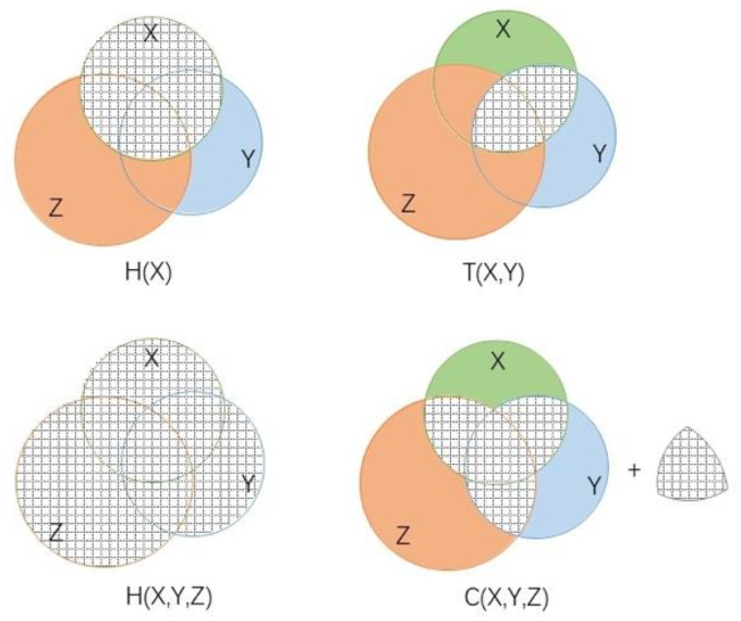
The joint entropy denotes the comprehensive information of two variables while the transformation denotes the information quantity shared by the two variables, i.e., mutual information, or the amount of redundant information between the two variables. The mutual information of X and Y is expressed as follows:
The redundant information [66] of a network comprising N rain gauges can be expressed by C, and the calculation expression is as follows:
Figure 3 shows the topological figures of the above indexes.
Regarding the data probability problem in the calculation of information entropy, we often compute the probability by setting different bin values for the discretization data because the calculation of the joint entropy of non-Gaussian distributions is relatively complex [16,25,67]. This paper applies the method of calculating the optimal bin value proposed by Scott [68]. The expression is as follows:
where is the standard deviation of an observation series of X (in this paper, this variable indicates the daily series of a rain gauge), and is the total number of a data series.
3.1.2. Entropy, Variance, and Standard Deviation
Variance and standard deviation in statistics and entropy in information theory can measure the amount of information of a group of random variables, and these parameters are widely used in some algorithms of machine learning and data mining. Variance and standard deviation measure the dispersion degree of a data distribution while information entropy measures the confusion degree and uncertainty degree of the data. Although the two are related to each other, they are not equivalent [69,70,71]. Variance is defined as the square of the data unit, which makes it difficult to interpret the numerical meaning, and it also exaggerates the dispersion degree of the data, which makes it difficult for people to intuitively understand the numerical significance. Therefore, the arithmetic square root of variance is usually taken as the indicator to describe the dispersion degree, i.e., the standard deviation.
3.2. Fundamental Theory of Kriging Interpolation
The kriging method is a widely used spatial interpolation method that was proposed by D. G. Krige, a mining engineer in South Africa (see [72]). Unlike the inverse distance weighting method and spline function method, which are directly based on the surrounding measured values or the degree of smoothness of the generated surface, the kriging method assigns different weights to each sampling point according to the spatial position and correlation by analyzing the spatial distribution of the variation in sampling point data. Subsequently, the estimated value of the interpolated point is obtained via a sliding weighted average, and the expression is as follows:
where is the estimated value at and is the weight coefficient, which satisfies the minimum error and unbiased estimation of the estimated value and the real value:
Different kriging interpolation methods rely on different assumptions. For example, ordinary kriging interpolation assumes that spatial attributes are homogeneous and have the same expectations and variances for any point in space. That is, the values at any point comprise the mean value and the random deviation of that point. Half of the variance of the difference between the values of x and x + h of the regionalized variable z(x) is defined as the semivariance function. The semivariance function values of different distances h are calculated as follows:
Generally, the fitting models of the semivariance function include the circle model, spherical model, exponential model, Gauss model and linear model. Kriging variance can be calculated by a semivariogram function, and the expression is as follows:
3.3. Optimization of Network Design
The optimal rain gauge network design consists of two parts: the identification of potential sites and the selection of the optimal site network.
3.3.1. Filtering Potential Stations
Potential stations are the locations where stations are expected to be built. The screening for potential stations involves the selection of areas within the study area as potential site layout areas. Previous rain-measuring station network layout designs primarily divided the whole research area according to a certain grid and then considered all grids as potential candidate stations directly [22,43], or manually selected individual grids as potential points according to the kriging interpolation accuracy (kriging variance) and other constraints [32,73]. The former requires considerable redundant calculations, especially for large study areas, and data with high spatial and temporal resolution; thus, this method is often used with radar data [43]. The latter manual screening method selects relatively fewer potential sites; thus, it is not conducive to the overall planning of a regional network.
Rainfall is a hydrological variable with significant spatial and temporal characteristics; therefore, the lack of existing networks and spatiotemporal characteristics of the site should be considered in the selection of potential sites. In practical applications, the kriging interpolation accuracy of the existing ground precipitation measurement stations can indicate whether the existing network needs to be supplemented [22,32,74]. In addition, remote sensing products provide more accurate relative spatial characteristics and temporal continuity, and thus can objectively represent local spatiotemporal characteristics [42].
When considering local spatiotemporal characteristics (window is z × z), because the number of local grids is small and the data changes are relatively single, the local spatial dispersion degree, i.e., the spatial characteristics, is more conveniently explained using variance rather than entropy based on the computational complexity and information accuracy. The changes of local spatial characteristics in a time series represent the required spatiotemporal characteristics, which can be obtained by calculating the entropy of the standard deviation in time series l, namely, the spatiotemporal information . A larger value of corresponds to regional spatiotemporal characteristics with greater significance and a greater number of rain observation stations required for control.
In summary, the expression for the screening for potential stations is as follows:
where denotes the local spatiotemporal information of the grid X in local window z in the time series; denotes the average kriging variance of grid X in time series l; and t denotes the threshold. Using “and” to connect the two screening conditions logically ensures that potential stations with considerable spatiotemporal information will be selected and indicates that accurate rainfall values cannot be obtained from the existing network. The qualified points are used as potential stations for subsequent optimized network design.
3.3.2. Optimized Conditions
The ideal optimal design scheme should add, remove, and change as little as possible based on the premise of maintaining the original network. Generally, because existing stations have a long time series of observation data and high data integrity, which are conducive to follow-up scientific research and actual situation analyses, it is recommended not to remove or change the existing stations when the station network is insufficient. This condition would ensure that the application requirements are met to maintain continuous observations when optimizing the design of the network. Several studies have also illustrated this perspective [16].
Assuming that the network has n sites, which is expressed as , according to the description above, m potential sites have been screened, which are expressed as . We consider that the new rain gauge network needs to meet the following three criteria after adding the stations:
(1) Maximizing the total information content of the network in time series , including maximizing the joint entropy, which ensures that the network can capture enough information from the time series data in the study area; (2) maximizing the mutual information between the network and the other stations that are not selected, which ensures that the selected network covers the time series information characteristics of the unselected stations as much as possible and (3) minimizing information redundancy within the network, which ensures minimum information duplication among stations in the network. Inspired by the MIMR method [28], is expressed as follows:
According to previous studies [28,32], the tradeoff weight is set to provide the user with the option to consider additional knowledge; in this paper, this value is set to 0.9.
Maximizing the spatiotemporal of the network ensures that the spatial characteristics of rainfall in the area are fully captured. The calculated indicator is the mean of the of all stations in the network based on remote sensing data. The higher the average spatiotemporal information of the rain gauge network, the stronger the spatiotemporality of precipitation captured by the whole site network. The expression of is as follows:
Maximizing the interpolation accuracy of the network , i.e., minimizing the regional kriging variance, ensures the accuracy of the network in the application. The expression of the is as follows:
where k is the number of grids in the study area.
In summary, the conditional expressions for the new network are as follows:
3.3.3. Greedy Ranking Algorithm
The greedy ranking algorithm is a common and simple ranking method that can transform a multi-objective problem into a single-objective problem and simplify the calculation process [28,32]. The three optimization objectives have a defined relationship and mutual influence. To avoid differences between different dimensions, the min-max normalization of the variables is performed before the greedy ranking algorithm is used. Taking the total information content as an example, the expression is as follows:
where and represent the maximum and minimum values of the total information content in the sequence of all potential sites added in the original network, respectively. The final expression of the optimization objective of the greedy ranking algorithm is as follows:
This expression is defined as the best ISA rules, whereby potential sites are added to the network in turn. In theory, as the number of stations increases, the total information content, spatial index, and errors of the network converge to a stable value [22,43,75].
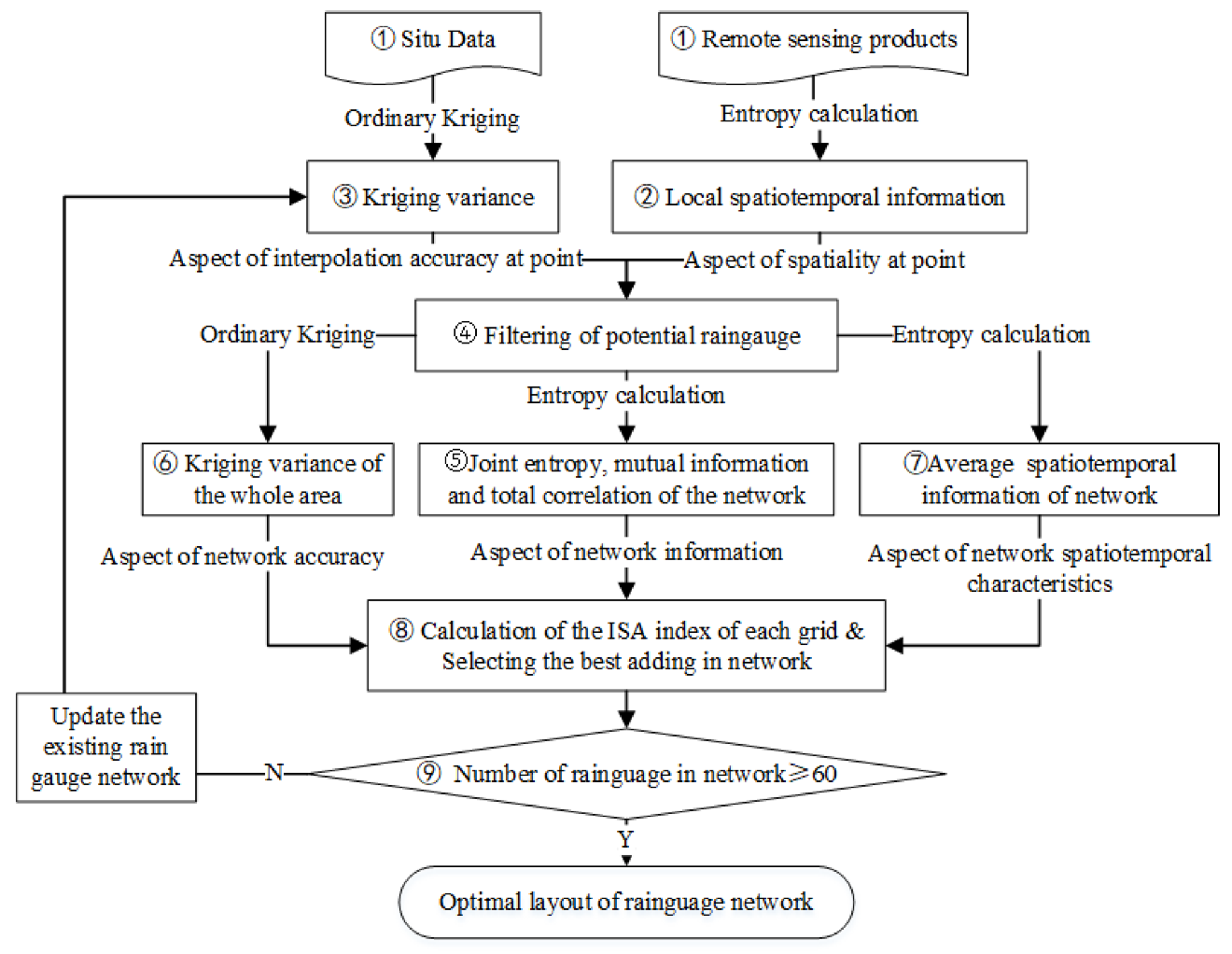
In summary, the detailed algorithm steps are as follows (corresponding flow chart is shown in Figure 4). Steps 2–4, from the perspective of the site location of the spatiotemporality and the degree of demand, implement the potential site selection and filter out the parts to improve the efficiency of the subsequent filter network. Steps 6–8, from the perspective of the network of comprehensive information content, spatiotemporality, and accuracy, filter out the best station network. The advantages of measured data and remote sensing data are applied synthetically to design the station network reasonably.
- Collect the time series data and remote sensing precipitation products for the existing stations in the study area and remove the abnormal data.
- Calculate at X in window z × z based on the time series data of remote sensing precipitation products.
- Perform kriging interpolation and determine the kriging variance of each grid in the study area based on the existing measured site data.
- Count the potential point sets satisfying the conditions throughout the area using Equation (11).
- Calculate the information content of each potential point after joining the network according to Equation (12).
- Calculate the average spatiotemporality of the station network after each potential point joins the network according to Equation (13).
- Calculate the average kriging variance of the study area after each potential point joins the network according to Equation (14).
- Calculate the ISA index according to Equation (17) after normalizing the deviation of three attribute values of each potential point and eliminating the influence of dimension, and then select the potential point with the maximum comprehensive attribute value to join the network.
- Repeat steps 3–8 until the number of stations in the network meets the preset number.
4. Results and Discussion
4.1. Result of the Network Design
4.1.1. Computation and Distribution of Entropy
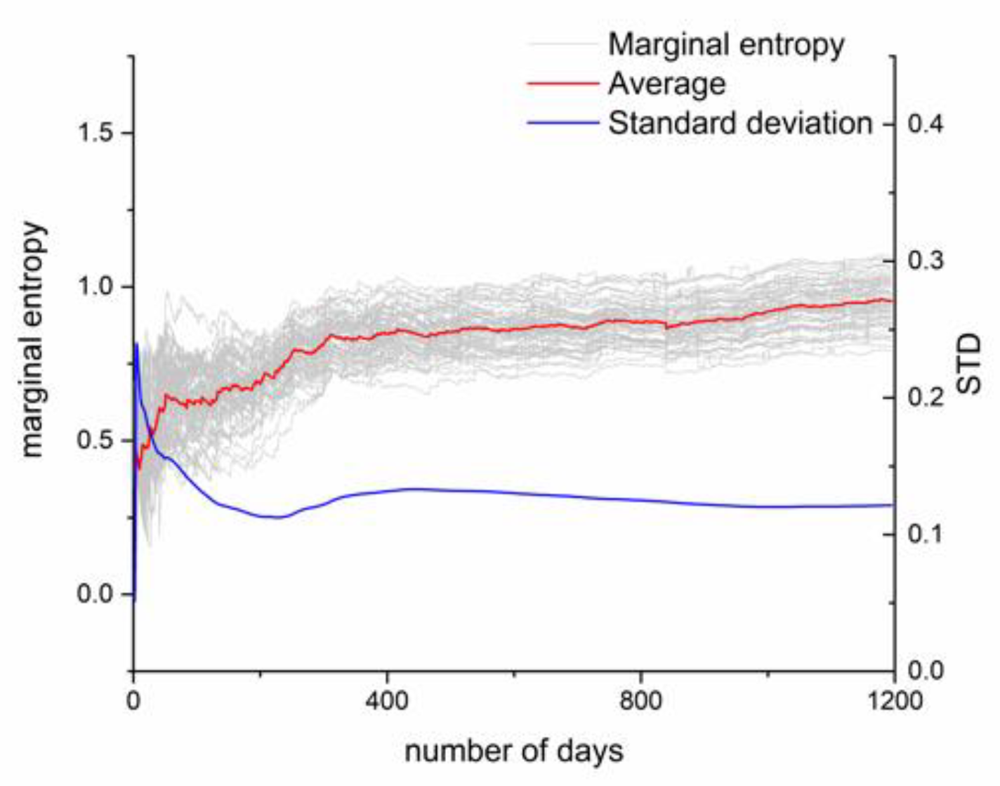
Keum and Coulibaly [16] concluded that a data sequence could provide comprehensive information for at least 10 years when the entropy method is applied to network design research using different time series lengths. The time series of this paper represents 10 years of rainy seasons, with each rainy season lasting for 5 months. After screening, the time series includes a total of 1196 days. The marginal entropy of a unit ranges from 0 to log2 (1196) = 10.22 bits. Because of the frequent precipitation during the rainy season, the amount of information is relatively small. Figure 5 shows the change in entropy with increasing time series length. The marginal entropy tends to be stable after it increases. Obviously, when the time is shorter than 300 days, the change in information entropy is significant and the variance is correspondingly high, which indicates that only 1 or 2 years of data are insufficient to capture the complete information. After a time series of 500 days is reached, the standard deviation of the marginal entropy decreases to 0.1. The information value of each point tends to be stable, which can represent all the changes at the point over time. This result shows that the selected time series can satisfy the information entropy calculation requirements and suggests that a time series during the rainy season shorter than 10 years may be applied to the design of a network with reasonable results.
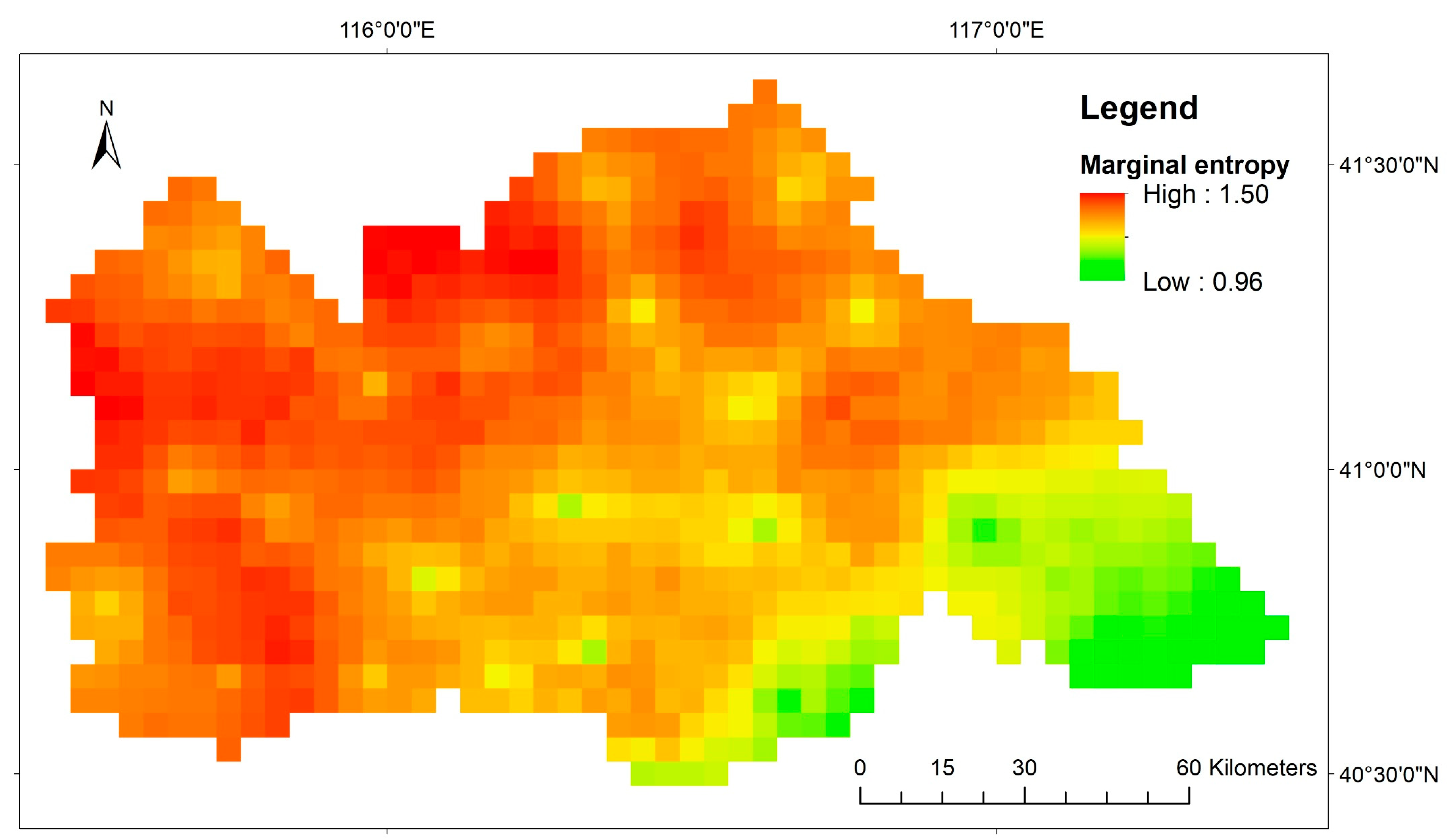
The spatial distribution of marginal entropy is calculated using the interpolation data of 25 randomly selected rain gauges, as shown in Figure 6. The marginal entropy in the map is high in the north and low in the south, and the relative elevation in the high-entropy area is also high. The high-entropy grids indicate that the precipitation has strong temporal variability and contains special information in particular grids. However, as described in reference [2], the grids with high entropy are not necessarily the best location for adding a rain gauge because the establishment of the network considers the comprehensive network information rather than the information of a single site.
4.1.2. Screening for Potential Stations
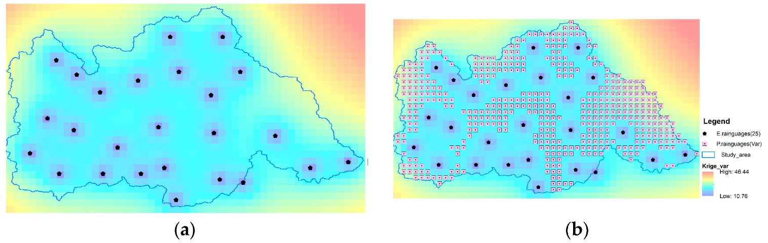
This paper describes the process of screening potential stations, and the screening event of the 26th rain gauge is considered as an example. As stated in Equation (12), the main objective is to screen for regions with inaccurate interpolation results and high local spatial heterogeneity. When screening, we tend to conduct a general screening because being too strict will lead to inadequate site candidates and being too loose will decrease the significance of the screening. Therefore, the thresholds of and are the 0.5 quantiles.
Figure 7a shows the distribution map from the interpolation results based on 25 observed rain gauges. The variance increases radially from the location of the existing observation rain gauge to the edge of the study area. Figure 7b shows the potential station area screened when the kriging variance threshold equals the 0.5 quantile. Potential station areas are distributed in all areas except around the observation station.
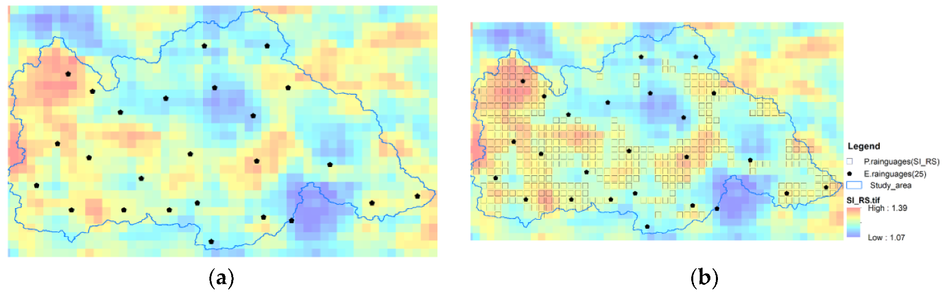
Figure 8a shows the distribution calculated from the remote sensing data. The chart shows that the value is high in the central and western parts of the study area, which means that the spatial heterogeneity is strong and that the consistency is considerable in the eastern part. This feature is also consistent with the elevation. Figure 8b shows the screening results of potential stations when the threshold value equals the 0.5 quantile, and the results are distributed mostly in the west and central regions.
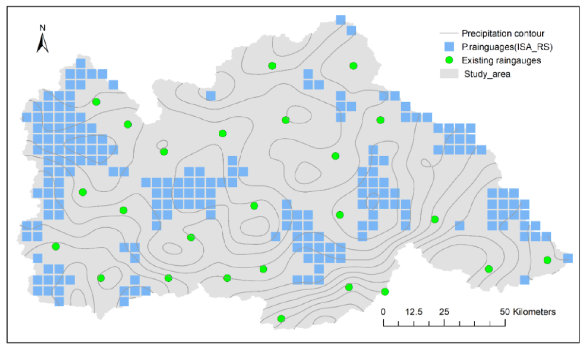
The two results are calculated logically, and the distribution of potential locations for the 26th rain gauge is obtained. We obtained 230 grids in total as shown in Figure 9. As the number of stations in the network increases, the number of potential grids for the additional station decreases gradually. For example, the result of the screening for potential new station locations for the 60th rain gauge is 165 grids.
4.1.3. Optimal Network of Additional Stations
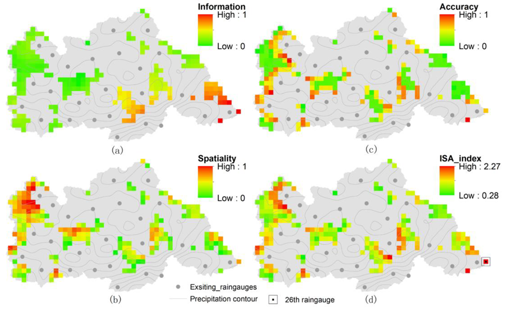
After screening out the potential rain gauge area, the best comprehensive station scenario is obtained according to the performance of the potential rain gauge when joining the rain gauge network, i.e., according to Equation (18). Figure 10 shows the results of screening for the 26th rain gauge.
Figure 10a shows that the distribution of the total information content of the network is low in the west and high in the east after a new rain gauge is added. The interpolation data based on the measured data suggest that additional stations in the south and east can enrich the rainfall data obtained by the network. Spatiotemporal information from the new network based on remote sensing data (Figure 10b) describes the local spatiotemporal characteristics collected by the network. The addition of stations in the eastern, central and western regions can help the network capture more spatial information, which is similar to the results of the precipitation contour map. Figure 10c shows that the kriging variance of the station network interpolation is uniformly distributed with the original network, and the best result is obtained when the network is sparse or along the edge. Based on the calculation results of the three aspects, the ISA distribution map (Figure 10d) is obtained and the maximum value is taken as the location of the 26th rain gauge according to the greedy algorithm.
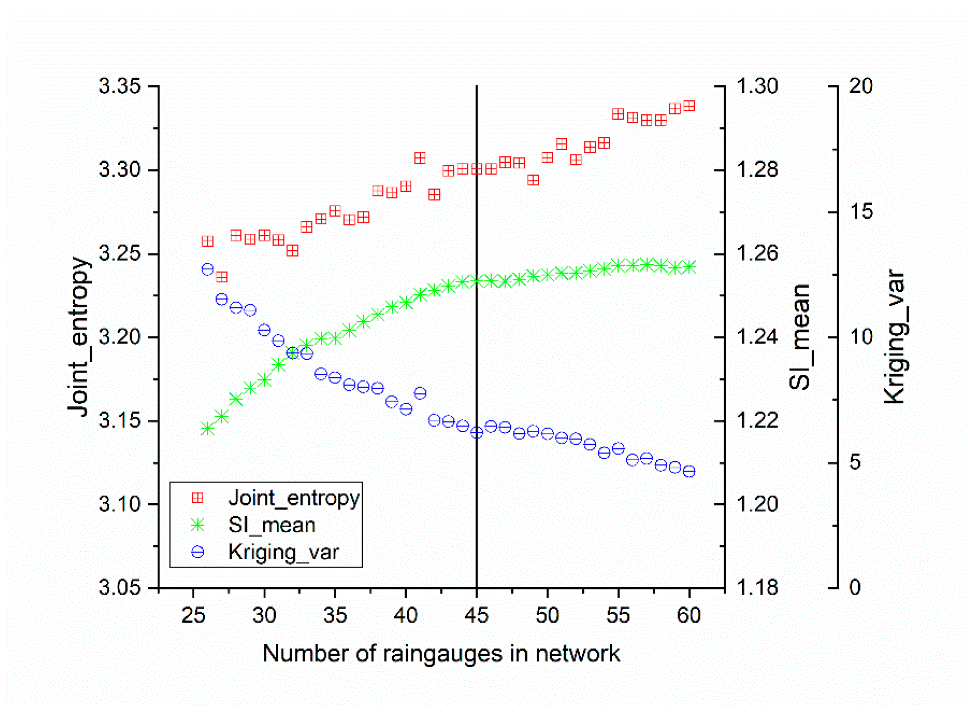
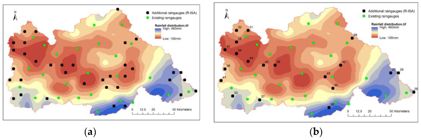
In this paper, the network results are calculated in turn until the total number of rain gauges is 60. With the increase in the number of stations, the total information, spatiality, and kriging variance of the network gradually stabilizes. The statistical results are shown in Figure 11, which shows that after adding 15–20 rain gauges, i.e., when the total number of rain gauges is approximately 45, the indicators of the rain gauge network no longer improve with the inclusion of additional rain gauges. In practice, the choice of how many rain gauges to add can be facilitated based on the statistical results. The network design results for 60 rain gauges and 45 rain gauges are shown in Figure 12.
4.2. Comparison and Verification of Index Selection
The network design results of this paper were compared with the results from a method that only considers the total information content and the kriging interpolation accuracy of the network for the network design. This method does not conduct potential point screening; in other words, all points in the study area are regarded as potential rain gauges. For convenience of expression, the method in this paper is abbreviated as R-ISA and the comparison method is abbreviated as S-IA. The optimized expression of S-IA method is
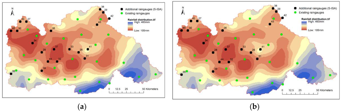
The design results are shown in Figure 13.
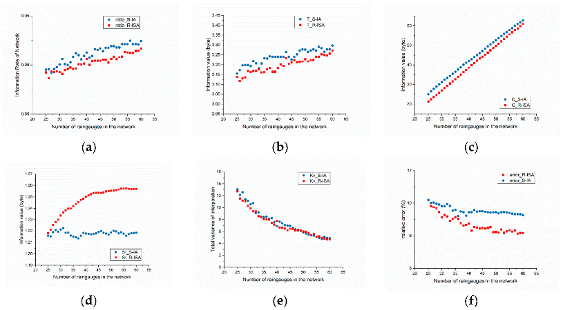
Regarding the intuitive layout, the distribution of the S-IA network is more uniform with the additional rain gauges located in the south-central part, which has fewer existing rain gauges, whereas the distribution of the R-ISA network appears to be more consistent with the precipitation distribution compared with the S-IA network. Figure 14 is obtained by calculating the statistics for various types of information, spatiality, and errors of the two networks.
Figure 14a–c mainly compare the performance of the two network design methods in terms of time series information. The results of the S-IA method are slightly better than those of the R-ISA method in terms of the proportion of joint entropy and the amount of information covered by the potential set of stations. The proportion of joint entropy reached approximately 90% after approximately 10 rain gauges were added. Figure 14b shows that the mutual information of the R-ISA network is slightly lower than that of the S-IA network with the increase in the number of stations. This result may be related to the fact that the S-IA method provides more potential stations than the R-ISA method. The redundancy of information within the R-ISA network is slightly higher than that within the S-IA network, which can be explained by the layout characteristics. The layout results of the S-IA method are relatively intensive in some areas, especially the southeast, compared with the R-ISA method, which affects the redundancy within the network. Significant differences in the spatial characteristics of the two networks are shown in Figure 14d.
As the number of S-IA networks increases, the SI (spatiotemporal information) value does not change significantly, indicating that the spatiotemporal information captured by the S-IA network does not increase significantly. In the screening of the R-ISA network, local spatiotemporal properties are taken into account, and the SI value shows an upward trend and tends to be stable. This difference in results is because the S-IA method focuses too much on the numerical differences in the time series of the interpolated measured data during network screening and does not consider local spatiotemporal changes in the network.
Figure 14e,f compare the accuracy of the two networks. Figure 14e shows the variation trend of the total variance of the average daily kriging interpolation throughout the screening process. Both networks decrease to the same extent as the number of stations increases. Figure 14f shows the variation in the average relative error compared with the true value and indicates that the resulting errors of this method are lower than those of the S-IA method. This result is closely related to the distribution of stations. With the same number of stations, the distribution of the R-ISA method is more balanced with the precipitation distribution than that of the S-IA, which may be based on the higher rainfall in the southeast region and significant spatiotemporal characteristics in the western region. The comparison of the results indicates that it is practical and effective to consider spatiality in the design of rain gauge networks.
4.3. Comparison and Verification of Data Selection
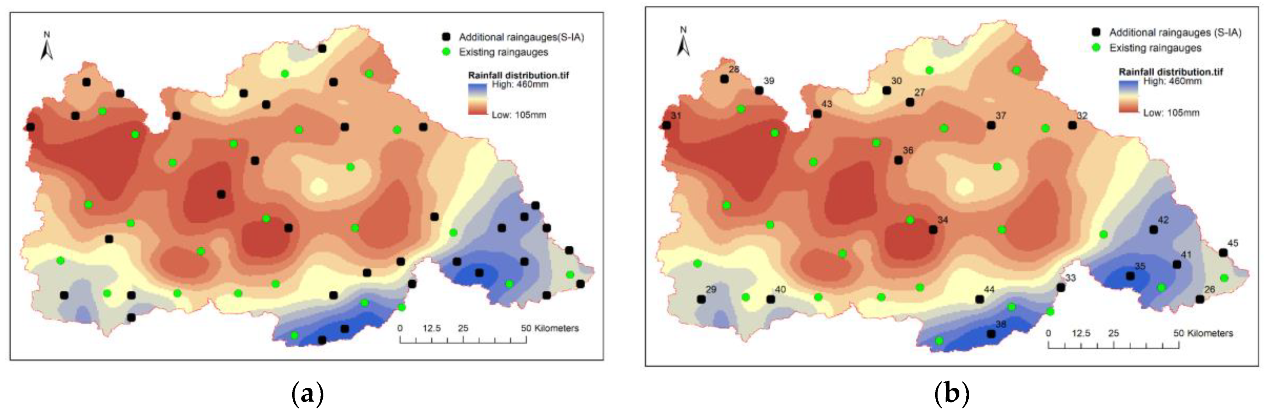
In this section, the same rules for potential point screening and site network screening are used to compare the results of the optimized station network design using the method proposed in this paper (R-ISA) and the method using only measured data (S-ISA). The optimized expression of S-ISA method is as follows:
where represents the spatiotemporal information calculated based the existing site network interpolation data.
Similarly, screening for a potential site for the 26th rain gauge is taken as an example. The distribution obtained by the S-ISA method is shown in Figure 15. Because the interpolation data are derived from adjacent grids, although a semivariogram is used in the interpolation, the spatiotemporal information response is not uniform when the density of the station network is not sufficiently large. The spatiotemporal information is high in places with high site density and low in places far from the existing stations, which is contrary to the conditions for the design of the station network. This result is also the basic defect of point-scale data interpolation for surface-scale data. Finally, the potential distribution results obtained by the S-ISA method combined with the two screening conditions are relatively concentrated (Figure 16). In contrast, remote sensing rainfall products are retrieved from spatial features, which are more objective and reasonable for the exchange of spatial information.
Figure 17 shows the results of the S-ISA method for the optimum design of the rain gauge network. Intuitively, the network selected by the S-ISA method is too concentrated in the area with better interpolation accuracy, and no sites are distributed on the edge of the area with few monitoring sites in the eastern part of the research area.
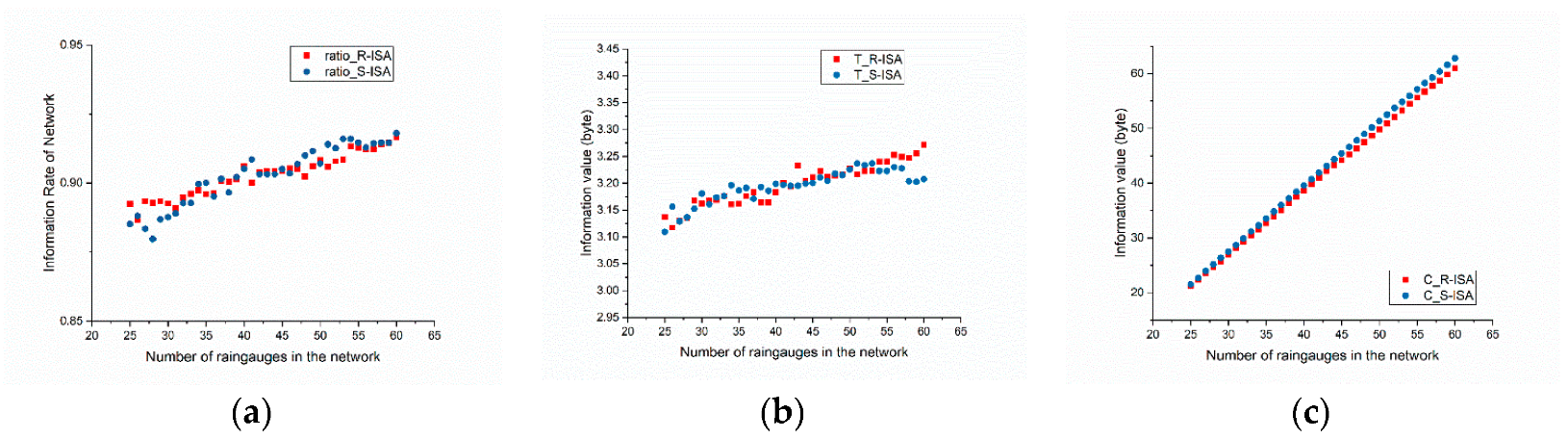
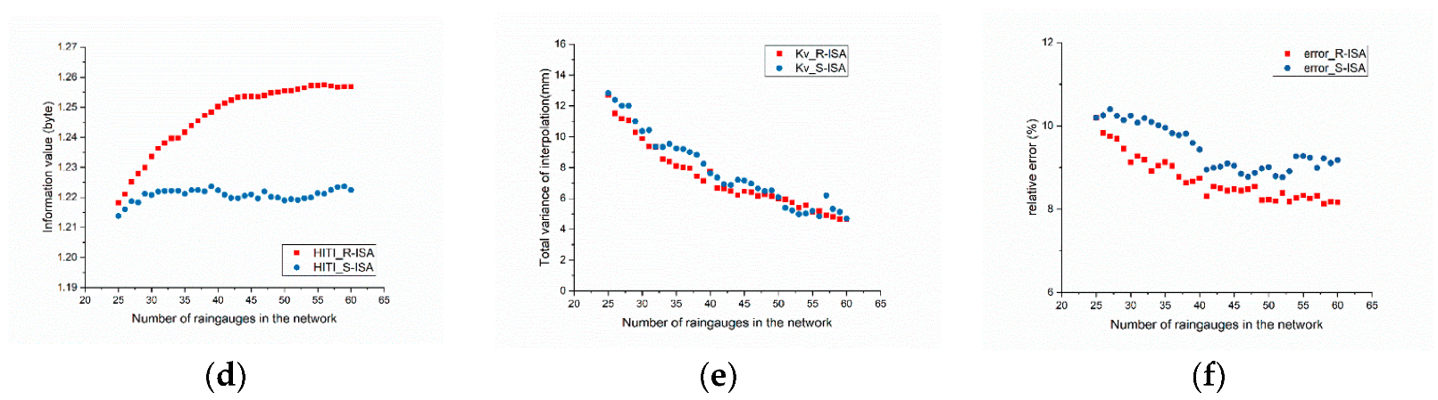
Figure 18, which is similar to Figure 14 in the previous section, is based on the performance of the two methods.
Figure 18a,b show that significant differences do not occur between the two networks in the proportion of joint entropy and transformation of residual potential stations, which may be related to the control of the same rainfall contour region by the two networks. In Figure 18c, because the stations are relatively concentrated in the middle, the S-ISA network is slightly higher than the R-ISA network in terms of the redundancy in the network.
Figure 18d demonstrates that as the number of stations increases, the SI value of the S-ISA method slightly increases and then decreases. This is because the spatiotemporality calculated based on the measured data is more accurate in the region with higher interpolation accuracy (that is, in the middle of the study area). However, as for the whole research area, accurate spatiotemporality cannot be obtained. Therefore, with the increase of rain gauges, the spatiotemporal information of the network is not significantly improved. Therefore, compared with R-ISA, this method cannot obtain accurate spatiotemporal properties for the whole area, and the spatiality of the R-ISA network is also superior to that of the S-ISA network. Although the difference in the mean variance of kriging interpolation between the two methods in Figure 18e fluctuates and is not very significant, the error optimization speed of the R-ISA method is faster and higher than that of the S-ISA method based on the relative errors (Figure 18f). A comprehensive comparison indicates that the results of a rain gauge network that considers spatiotemporality based on satellite rainfall products are more advantageous in terms of spatiotemporality and accuracy than those considering spatiotemporality based on interpolation data.
5. Summary and Conclusions
In this paper, a method for optimizing the design of rain gauge networks using both remote sensing and measured data is presented. The design process involves two parts: potential rain gauge screening and network screening. Potential rain gauge screening refers to screening out areas that are most in need of stations by considering the point perspective of high kriging accuracy of the measured data and low local spatial flux based on remote sensing data. In contrast, network screening refers to selecting the best combination of rain gauges from the potential rain gauges from the perspective of the network. This part of the method mainly considers three indicators that are of high degree: the total information content of the network, the spatiotemporality of the network, and the interpolation accuracy of the network. The information content and accuracy are calculated from ground-measured data. The information calculations include the joint entropy of the network, the mutual information outside the network, and the redundancy inside the network. The SI is calculated from remote sensing data to reflect the spatial and temporal characteristics of the network. The accuracy of the network is represented by the kriging variance of interpolation. Then, the greedy algorithm is used to rank the rain gauges in the network. This approach ensures the appropriate design of station networks by leveraging the high accuracy of measured data and the good spatiality of remote sensing data.
This paper compares the results of the proposed method with that of two other methods that consider only two indicators (information content and kriging variance) (S-IA) and all three indicators but only in situ data (S-ISA). The results of the S-IA method show that the distribution of stations is too uniform because the spatial representativeness is not considered. The distribution of stations in the S-ISA results is too centralized because the spatial interpolation of the measured data is quite different in the middle and edge regions. The R-ISA results retain the advantages of the S-IA method. Moreover, the introduction of remote sensing data into the calculation space is more objective and performs better in all aspects. However, due to the use of two types of data sources, this method is still subject to the limitation of spatial scale and a certain degree of uncertainty; moreover, remote sensing data still need to be cleaned before they can be used in this application. In summary, the rain gauge network design method combined with the satellite data proposed in this paper can not only ensure the content of information and application accuracy obtained by the network but also ensure the ability of the station network to capture spatial features and provide satellite remote sensing data to assist with the design of ground station networks as a new solution. In addition, through the two steps, potential point screening and station network screening, the efficiency of the station network optimization is improved.
Furthermore, there are still some research problems in this paper, such as how to better leverage the advantages of remote sensing data when combined with other hydrological elements, the analysis of the difference between the results of the greedy algorithm and the results of the multi-objective optimization algorithm described in the literature and the influence of the scale of remote sensing data on the design of the rain gauge network.
Author Contributions
Conceptualization, Y.H., H.Z. and Y.J.; Data curation, Y.H. and X.L.; Formal analysis, Y.H. and H.Z.; Funding acquisition, H.Z. and Y.J.; Investigation, Y.H., H.Z. and X.L.; Methodology, Y.H. and Y.J.; Project administration, H.Z. and Y.J.; Resources, H.Z. and Y.J.; Software, Y.H. and X.L.; Supervision, X.L.; Validation, Y.H. and X.L.; Visualization, X.L.; Writing—original draft, Y.H.; Writing—review and editing, Y.H. All authors have read and agreed to the published version of the manuscript.
Funding
This research was funded by the National Key Research and Development Program of China (No. 2018YFC0407705), Special Project of Basic Scientific Research of China Institute of Water Resources and Hydropower Research (No. WR0145B012017) and Special Project of Science and Technology Achievement Conversion Fund of China Institute of Water Resources and Hydropower Research (No. WR1003A112016).
Acknowledgments
We would like to thank the journal editors and anonymous reviewers for their comments, which have helped to improve the original manuscript. The measured precipitation data used in this study are derived from the basic measured precipitation data provided by the Hydrologic Yearbook of China. The satellite remote sensing precipitation data is from PERSIANN-CCS, released by Hong Yang et al. (website: http://chrsdata.eng.uci.edu/). Thank you to all of the relevant agencies for providing the data.
Conflicts of Interest
The authors declare no conflict of interest.
References
- WMO. Guide to Hydrological Practices. Volume I. Hydrology—From Measurement to Hydrological Information; World Meteorological Organization (WMO) Geneva: Geneva, Switzerland, 2008. [Google Scholar]
- Kornelsen, K.C.; Coulibaly, P. Design of an optimal soil moisture monitoring network using SMOS retrieved soil moisture. IEEE Trans. Geosci. Remote Sens. 2015, 53, 3950–3959. [Google Scholar] [CrossRef]
- Joshi, N.; Baumann, M.; Ehammer, A.; Fensholt, R.; Grogan, K.; Hostert, P.; Jepsen, M.R.; Kuemmerle, T.; Meyfroidt, P.; Mitchard, E.T. A review of the application of optical and radar remote sensing data fusion to land use mapping and monitoring. Remote Sens. 2016, 8, 70. [Google Scholar] [CrossRef] [Green Version]
- Mishra, A.K.; Coulibaly, P. Developments in hydrometric network design: A review. Rev. Geophys. 2009, 47. [Google Scholar] [CrossRef]
- Chacon-Hurtado, J.C.; Alfonso, L.; Solomatine, D.P. Rainfall and streamflow sensor network design: A review of applications, classification, and a proposed framework. Hydrol. Earth Syst. Sci. 2017, 21, 1–33. [Google Scholar] [CrossRef] [Green Version]
- Silverman, B.A.; Koshio Rogers, L.; Dahl, D. On the sampling variance of raingage networks. J. Appl. Meteorol. 1981, 20, 1468–1478. [Google Scholar] [CrossRef] [Green Version]
- Morrissey, M.L.; Maliekal, J.A.; Greene, J.S.; Wang, J. The uncertainty of simple spatial averages using rain gauge networks. Water Resour. Res. 1995, 31, 2011–2017. [Google Scholar] [CrossRef]
- Maddock, T., III. An optimum reduction of gauges to meet data program constraints. Hydrol. Sci. J. 1974, 19, 337–345. [Google Scholar] [CrossRef]
- Huff, F. Sampling errors in measurement of mean precipitation. J. Appl. Meteorol. 1970, 9, 35–44. [Google Scholar] [CrossRef]
- Ali, M.Z.M.; Othman, F. Raingauge network optimization in a tropical urban area by coupling cross-validation with the geostatistical technique. Hydrol. Sci. J. 2018, 63, 474–491. [Google Scholar] [CrossRef]
- Skok, G. Analytical and practical examples of estimating the average nearest-neighbor distance in a rain gauge network. Meteorol. Z. 2006, 15, 565–573. [Google Scholar] [CrossRef]
- Basist, A.; Bell, G.D.; Meentemeyer, V. Statistical relationships between topography and precipitation patterns. J. Clim. 1994, 7, 1305–1315. [Google Scholar] [CrossRef]
- Chebbi, A.; Bargaoui, Z.K.; Cunha, M.D.C. Optimal extension of rain gauge monitoring network for rainfall intensity and erosivity index interpolation. J. Hydrol. Eng. 2011, 16, 665–676. [Google Scholar] [CrossRef]
- Leach, J.M.; Coulibaly, P.; Guo, Y. Entropy based groundwater monitoring network design considering spatial distribution of annual recharge. Adv. Water Resour. 2016, 96, 108–119. [Google Scholar] [CrossRef]
- Ridolfi, E.; Rianna, M.; Trani, G.; Alfonso, L.; Baldassarre, G.D.; Napolitano, F.; Russo, F. A new methodology to define homogeneous regions through an entropy based clustering method. Adv. Water Resour. 2016, 96, 237–250. [Google Scholar] [CrossRef]
- Keum, J.; Coulibaly, P. Information theory-based decision support system for integrated design of multivariable hydrometric networks. Water Resour. Res. 2017, 53, 1–21. [Google Scholar] [CrossRef]
- Shannon, C.E. A mathematical theory of communication. Bell Syst. Tech. J. 1948, 27, 379–423. [Google Scholar] [CrossRef] [Green Version]
- Amorocho, J.; Espildora, B. Entropy in the assessment of uncertainty in hydrologic systems and models. Water Resour. Res. 1973, 9, 1511–1522. [Google Scholar] [CrossRef]
- Caselton, W.F.; Husain, T. Hydrologic networks: Information transmission. J. Water Resour. Plan. Manag. Div. 1980, 106, 503–520. [Google Scholar]
- Krstanovic, P.; Singh, V. Evaluation of rainfall networks using entropy: I. Theoretical development. Water Resour. Manag. 1992, 6, 279–293. [Google Scholar] [CrossRef]
- Krstanovic, P.; Singh, V. Evaluation of rainfall networks using entropy: II. Application. Water Resour. Manag. 1992, 6, 295–314. [Google Scholar] [CrossRef]
- Chen, Y.C.; Wei, C.; Yeh, H.C. Rainfall network design using kriging and entropy. Hydrol. Process. 2008, 22, 340–346. [Google Scholar] [CrossRef]
- Yeh, H.-C.; Chen, Y.-C.; Wei, C.; Chen, R.-H. Entropy and kriging approach to rainfall network design. Paddy Water Environ. 2011, 9, 343–355. [Google Scholar] [CrossRef]
- Alfonso, L.; He, L.; Lobbrecht, A.; Price, R. Information theory applied to evaluate the discharge monitoring network of the Magdalena River. J. Hydroinformatics 2013, 15, 211–228. [Google Scholar] [CrossRef] [Green Version]
- Alfonso, L.; Lobbrecht, A.; Price, R. Information theory-based approach for location of monitoring water level gauges in polders. Water Resour. Res. 2010, 46, 374–381. [Google Scholar] [CrossRef]
- Alfonso, L.; Lobbrecht, A.; Price, R. Optimization of water level monitoring network in polder systems using information theory. Water Resour. Res. 2010, 46, 595–612. [Google Scholar] [CrossRef]
- Samuel, J.; Coulibaly, P.; Kollat, J. CRDEMO: Combined regionalization and dual entropy-multiobjective optimization for hydrometric network design. Water Resour. Res. 2013, 49, 8070–8089. [Google Scholar] [CrossRef]
- Li, C.; Singh, V.P.; Mishra, A.K. Entropy theory-based criterion for hydrometric network evaluation and design: Maximum information minimum redundancy. Water Resour. Res. 2012, 48, 5521. [Google Scholar] [CrossRef]
- Keum, J.; Coulibaly, P. Sensitivity of entropy method to time series length in hydrometric network design. J. Hydrol. Eng. 2017, 22, 04017009. [Google Scholar] [CrossRef]
- Wang, W.; Wang, D.; Singh, V.P.; Wang, Y.; Wu, J.; Wang, L.; Zou, X.; Liu, J.; Zou, Y.; He, R. Optimization of rainfall networks using information entropy and temporal variability analysis. J. Hydrol. 2018, 559, 136–155. [Google Scholar] [CrossRef]
- Xu, H.; Xu, C.-Y.; Sælthun, N.R.; Xu, Y.; Zhou, B.; Chen, H. Entropy theory based multi-criteria resampling of rain gauge networks for hydrological modelling–A case study of humid area in southern China. J. Hydrol. 2015, 525, 138–151. [Google Scholar] [CrossRef]
- Xu, P.; Wang, D.; Singh, V.P.; Wang, Y.; Wu, J.; Wang, L.; Zou, X.; Liu, J.; Zou, Y.; He, R. A kriging and entropy-based approach to raingauge network design. Environ. Res. 2018, 161, 61–75. [Google Scholar] [CrossRef] [PubMed]
- Ashouri, H.; Hsu, K.-L.; Sorooshian, S.; Braithwaite, D.K.; Knapp, K.R.; Cecil, L.D.; Nelson, B.R.; Prat, O.P. PERSIANN-CDR: Daily precipitation climate data record from multisatellite observations for hydrological and climate studies. Bull. Am. Meteorol. Soc. 2015, 96, 69–83. [Google Scholar] [CrossRef] [Green Version]
- Li, Y.; Grimaldi, S.; Walker, J.P.; Pauwels, V. Application of remote sensing data to constrain operational rainfall-driven flood forecasting: A review. Remote Sens. 2016, 8, 456. [Google Scholar] [CrossRef] [Green Version]
- Hou, A.Y.; Kakar, R.K.; Neeck, S.; Azarbarzin, A.A.; Kummerow, C.D.; Kojima, M.; Oki, R.; Nakamura, K.; Iguchi, T. The global precipitation measurement mission. Bull. Am. Meteorol. Soc. 2014, 95, 701–722. [Google Scholar] [CrossRef]
- Joyce, R.J.; Janowiak, J.E.; Arkin, P.A.; Xie, P. CMORPH: A method that produces global precipitation estimates from passive microwave and infrared data at high spatial and temporal resolution. J. Hydrometeorol. 2004, 5, 487–503. [Google Scholar] [CrossRef]
- Sorooshian, S.; Hsu, K.-L.; Gao, X.; Gupta, H.V.; Imam, B.; Braithwaite, D. Evaluation of PERSIANN system satellite-based estimates of tropical rainfall. Bull. Am. Meteorol. Soc. 2000, 81, 2035–2046. [Google Scholar] [CrossRef] [Green Version]
- Adler, R.F.; Huffman, G.J.; Chang, A.; Ferraro, R.; Xie, P.-P.; Janowiak, J.; Rudolf, B.; Schneider, U.; Curtis, S.; Bolvin, D. The version-2 global precipitation climatology project (GPCP) monthly precipitation analysis (1979–present). J. Hydrometeorol. 2003, 4, 1147–1167. [Google Scholar] [CrossRef]
- Hong, Y.; Hsu, K.-L.; Sorooshian, S.; Gao, X. Precipitation estimation from remotely sensed imagery using an artificial neural network cloud classification system. J. Appl. Meteorol. 2004, 43, 1834–1853. [Google Scholar] [CrossRef] [Green Version]
- Shi, C.; Jiang, L.; Zhang, T.; Xu, B.; Han, S. Status and plans of CMA land data assimilation system (CLDAS) project. In Proceedings of the EGU General Assembly Conference Abstracts, Vienna, Austria, 27 April–2 May 2014. [Google Scholar]
- Syed, T.H.; Famiglietti, J.S.; Rodell, M.; Chen, J.; Wilson, C.R. Analysis of terrestrial water storage changes from GRACE and GLDAS. Water Resour. Res. 2008, 44. [Google Scholar] [CrossRef]
- Dai, Q.; Bray, M.; Zhuo, L.; Islam, T.; Han, D. A scheme for rain gauge network design based on remotely sensed rainfall measurements. J. Hydrometeorol. 2017, 18, 363–379. [Google Scholar] [CrossRef]
- Yeh, H.-C.; Chen, Y.-C.; Chang, C.-H.; Ho, C.-H.; Wei, C. Rainfall Network Optimization Using Radar and Entropy. Entropy 2017, 19, 553. [Google Scholar] [CrossRef] [Green Version]
- Wang, K.; Guan, Q.; Chen, N.; Tong, D.; Hu, C.; Peng, Y.; Dong, X.; Yang, C. Optimizing the configuration of precipitation stations in a space-ground integrated sensor network based on spatial-temporal coverage maximization. J. Hydrol. 2017, 548, 625–640. [Google Scholar] [CrossRef]
- Church, R.; ReVelle, C. The maximal covering location problem. Pap. Reg. Sci. 1974, 32, 101–118. [Google Scholar] [CrossRef]
- Hussain, M.; Chen, D.; Cheng, A.; Wei, H.; Stanley, D. Change detection from remotely sensed images: From pixel-based to object-based approaches. ISPRS J. Photogramm. Remote Sens. 2013, 80, 91–106. [Google Scholar] [CrossRef]
- Racoviteanu, A.; Williams, M.W. Decision tree and texture analysis for mapping debris-covered glaciers in the Kangchenjunga area, Eastern Himalaya. Remote Sens. 2012, 4, 3078–3109. [Google Scholar] [CrossRef] [Green Version]
- Walter, V. Object-based classification of remote sensing data for change detection. ISPRS J. Photogramm. Remote Sens. 2004, 58, 225–238. [Google Scholar] [CrossRef]
- Zhang, X.; Cui, J.; Wang, W.; Lin, C. A study for texture feature extraction of high-resolution satellite images based on a direction measure and gray level co-occurrence matrix fusion algorithm. Sensors 2017, 17, 1474. [Google Scholar] [CrossRef] [Green Version]
- Li, Z.; Shi, W.; Hao, M.; Zhang, H. Unsupervised change detection using spectral features and a texture difference measure for VHR remote-sensing images. Int. J. Remote Sens. 2017, 38, 7302–7315. [Google Scholar] [CrossRef]
- Hong, Y.; Gochis, D.; Cheng, J.-T.; Hsu, K.-L.; Sorooshian, S. Evaluation of PERSIANN-CCS rainfall measurement using the NAME event rain gauge network. J. Hydrometeorol. 2007, 8, 469–482. [Google Scholar] [CrossRef] [Green Version]
- Hong, Y.; Adler, R.F.; Negri, A.; Huffman, G.J. Flood and landslide applications of near real-time satellite rainfall products. Nat. Hazards 2007, 43, 285–294. [Google Scholar] [CrossRef] [Green Version]
- Hsu, K.-L.; Gao, X.; Sorooshian, S.; Gupta, H.V. Precipitation estimation from remotely sensed information using artificial neural networks. J. Appl. Meteorol. 1997, 36, 1176–1190. [Google Scholar] [CrossRef]
- Chiang, Y.-M.; Hsu, K.-L.; Chang, F.-J.; Hong, Y.; Sorooshian, S. Merging multiple precipitation sources for flash flood forecasting. J. Hydrol. 2007, 340, 183–196. [Google Scholar] [CrossRef] [Green Version]
- Nguyen, P.; Sellars, S.; Thorstensen, A.; Tao, Y.; Ashouri, H.; Braithwaite, D.; Hsu, K.; Sorooshian, S. Satellites track precipitation of super Typhoon Haiyan. Eos Trans. Am. Geophys. Union 2014, 95, 133–135. [Google Scholar] [CrossRef]
- Nguyen, P.; Thorstensen, A.; Sorooshian, S.; Hsu, K.; AghaKouchak, A. Flood forecasting and inundation mapping using HiResFlood-UCI and near-real-time satellite precipitation data: The 2008 Iowa flood. J. Hydrometeorol. 2015, 16, 1171–1183. [Google Scholar] [CrossRef]
- Zeweldi, D.A.; Gebremichael, M. Sub-daily scale validation of satellite-based high-resolution rainfall products. Atmos. Res. 2009, 92, 427–433. [Google Scholar] [CrossRef]
- Cánovas-García, F.; García-Galiano, S.; Karbalaee, N. Validation of a global satellite rainfall product for real time monitoring of meteorological extremes. In Remote Sensing for Agriculture, Ecosystems, and Hydrology XIX; International Society for Optics and Photonics: Warsaw, Poland, 2017; p. 1042109. [Google Scholar]
- Chang, F.-J.; Chiang, Y.-M.; Tsai, M.-J.; Shieh, M.-C.; Hsu, K.-L.; Sorooshian, S. Watershed rainfall forecasting using neuro-fuzzy networks with the assimilation of multi-sensor information. J. Hydrol. 2014, 508, 374–384. [Google Scholar] [CrossRef] [Green Version]
- Tao, Y.; Gao, X.; Ihler, A.; Hsu, K.; Sorooshian, S. Deep neural networks for precipitation estimation from remotely sensed information. In Proceedings of the 2016 IEEE Congress on Evolutionary Computation (CEC), Vancouver, BC, Canada, 24–29 July 2016. [Google Scholar]
- Sadeghi, M.; Asanjan, A.A.; Faridzad, M.; Nguyen, P.; Hsu, K.; Sorooshian, S.; Braithwaite, D. PERSIANN-CNN: Precipitation Estimation from Remotely Sensed Information Using Artificial Neural Networks–Convolutional Neural Networks. J. Hydrometeorol. 2019, 20, 2273–2289. [Google Scholar] [CrossRef]
- Hao, Z.; Singh, V.P. Single-site monthly streamflow simulation using entropy theory. Water Resour. Res. 2011, 47. [Google Scholar] [CrossRef]
- Ilunga, M. Shannon Entropy for Measuring Spatial Complexity Associated with Mean Annual Runoff of Tertiary Catchments of the Middle Vaal Basin in South Africa. Entropy 2019, 21, 366. [Google Scholar] [CrossRef] [Green Version]
- Keum, J.; Kornelsen, K.; Leach, J.; Coulibaly, P. Entropy Applications to Water Monitoring Network Design: A Review. Entropy 2017, 19, 613. [Google Scholar] [CrossRef] [Green Version]
- Zhu, Q.; Shen, L.; Liu, P.; Zhao, Y.; Yang, Y.; Huang, D.; Wang, P.; Yang, J. Evolution of the Water Resources System Based on Synergetic and Entropy Theory. Polish J. Environ. Stud. 2015, 24, 2727–2738. [Google Scholar] [CrossRef]
- Watanabe, S. Information theoretical analysis of multivariate correlation. IBM J. Res. Dev. 1960, 4, 66–82. [Google Scholar] [CrossRef]
- Fahle, M.; Hohenbrink, T.L.; Dietrich, O.; Lischeid, G. Temporal variability of the optimal monitoring setup assessed using information theory. Water Resour. Res. 2015, 51, 7723–7743. [Google Scholar] [CrossRef] [Green Version]
- Scott, D.W. On optimal and data-based histograms. Biometrika 1979, 66, 605–610. [Google Scholar] [CrossRef]
- Dionisio, A.; Menezes, R.; Mendes, D.A. Entropy and uncertainty analysis in financial markets. arXiv 2007, arXiv:0709.0668. [Google Scholar]
- Magidson, J. Qualitative variance, entropy, and correlation ratios for nominal dependent variables. Soc. Sci. Res. 1981, 10, 177–194. [Google Scholar] [CrossRef]
- Wei, Y. Variance, Entropy, and Uncertainty Measure; Dept. Stastistics, People’s Univ. China, 1987; pp. 609–610. [Google Scholar]
- Cressie, N. The origins of kriging. Math. Geol. 1990, 22, 239–252. [Google Scholar] [CrossRef]
- Mahmoudi-Meimand, H.; Nazif, S.; Ali Abbaspour, R.; Faraji Sabokbar, H. An algorithm for optimisation of a rain gauge network based on geostatistics and entropy concepts using GIS. J. Spat. Sci. 2016, 61, 233–252. [Google Scholar] [CrossRef]
- Chebbi, A.; Bargaoui, Z.K.; Abid, N.; da Conceição Cunha, M. Optimization of a hydrometric network extension using specific flow, kriging and simulated annealing. J. Hydrol. 2017, 555, 971–982. [Google Scholar] [CrossRef] [Green Version]
- Wei, C.; Yeh, H.-C.; Chen, Y.-C. Spatiotemporal scaling effect on rainfall network design using entropy. Entropy 2014, 16, 4626–4647. [Google Scholar] [CrossRef] [Green Version]
Figure 1.
Study area.

Figure 2.
Spatial distribution of the correlation coefficients for the measured precipitation data and remote sensing precipitation data.
Figure 2.
Spatial distribution of the correlation coefficients for the measured precipitation data and remote sensing precipitation data.

Figure 3.
Topological implications of different information entropies. The hatched areas denote the areas that correspond to the stated expressions.
Figure 3.
Topological implications of different information entropies. The hatched areas denote the areas that correspond to the stated expressions.

Figure 4.
Flowchart for the optimal design of a rain gauge network. ISA, information content, spatiotemporality, and accuracy.
Figure 4.
Flowchart for the optimal design of a rain gauge network. ISA, information content, spatiotemporality, and accuracy.

Figure 5.
Time statistics of marginal entropy.

Figure 6.
Spatial statistics of marginal entropy.

Figure 7.
Screening based on . (a) The spatial distribution of and (b) the 0.5 quantile potential station distribution based on quantile screening.
Figure 7.
Screening based on . (a) The spatial distribution of and (b) the 0.5 quantile potential station distribution based on quantile screening.

Figure 8.
Screening based on . (a) Spatial distribution of and (b) 0.5 quantile potential station distribution based on quantile screening.
Figure 8.
Screening based on . (a) Spatial distribution of and (b) 0.5 quantile potential station distribution based on quantile screening.

Figure 9.
Distribution of the potential positions of the 26th rain gauge.

Figure 10.
Screening for the 26th rain gauge. (a–d) are the distribution of the total information content, spatiotemporality, accuracy, and ISA components after potential points join the network.
Figure 10.
Screening for the 26th rain gauge. (a–d) are the distribution of the total information content, spatiotemporality, accuracy, and ISA components after potential points join the network.

Figure 11.
Statistics of the optimum design results for a station network of 60 rain gauges.

Figure 12.
Optimal design of the R-ISA method. (a) Network of 60 rain gauges and (b) network of 45 rain gauges.
Figure 12.
Optimal design of the R-ISA method. (a) Network of 60 rain gauges and (b) network of 45 rain gauges.

Figure 13.
Optimal design of the S-IA method. (a) Network of 60 rain gauges and (b) network of 45 rain gauges.
Figure 13.
Optimal design of the S-IA method. (a) Network of 60 rain gauges and (b) network of 45 rain gauges.

Figure 14.
Comparison of the R-ISA and S-IA methods. (a) Statistical diagram of the percentage of joint entropy of the network; (b) statistical diagram of mutual information between the network and potential station sets; (c) statistical diagram of the information redundancy of the network; (d) statistical diagram of the average spatiotemporal information of the network (SI); (e) statistical diagram of the daily mean kriging variance of the network and (f) statistical diagram of the relative errors of the network.

Figure 15.
Screening based on using measured data. (a) Spatial distribution of based on measured data and (b) 0.5 quantile potential station distribution from quantile screening based on measured data.
Figure 15.
Screening based on using measured data. (a) Spatial distribution of based on measured data and (b) 0.5 quantile potential station distribution from quantile screening based on measured data.

Figure 16.
Distribution of the potential positions of the 26th rain gauge using the S-ISA method.

Figure 17.
Optimal design of the S-ISA method. (a) Network of 60 rain gauges and (b) network of 45 rain gauges.
Figure 17.
Optimal design of the S-ISA method. (a) Network of 60 rain gauges and (b) network of 45 rain gauges.

Figure 18.
Comparison of the R-ISA and S-ISA methods. (a) Statistical diagram of the percentage of joint entropy of the network; (b) statistical diagram of mutual information between the network and potential station sets; (c) statistical diagram of the information redundancy of the network; (d) statistical diagram of the average SI of the network; (e) statistical diagram of the daily mean kriging variance of the network and (f) statistical diagram of the relative errors of the network.


Table 1.
Correlation coefficients between the measured precipitation and remote sensing precipitation time series data.
Table 1.
Correlation coefficients between the measured precipitation and remote sensing precipitation time series data.
| Correlation Coefficient | Amount of Time (Days) | Percentage of Total Time (%) | Cumulative Frequency (%) |
|---|---|---|---|
| Abnormal data | 141 | 9.22 | 9.22 |
| 0.0–0.1 | 16 | 1.05 | 10.27 |
| 0.1–0.3 | 77 | 5.03 | 15.30 |
| 0.3–0.5 | 100 | 6.54 | 21.84 |
| 0.5–0.7 | 140 | 9.15 | 30.99 |
| 0.7–0.9 | 191 | 12.48 | 43.47 |
| 0.9–1.0 | 865 | 56.53 | 100.00 |
© 2020 by the authors. Licensee MDPI, Basel, Switzerland. This article is an open access article distributed under the terms and conditions of the Creative Commons Attribution (CC BY) license (http://creativecommons.org/licenses/by/4.0/).
Share and Cite
MDPI and ACS Style
Huang, Y.; Zhao, H.; Jiang, Y.; Lu, X. A Method for the Optimized Design of a Rain Gauge Network Combined with Satellite Remote Sensing Data. Remote Sens. 2020, 12, 194. https://0-doi-org.brum.beds.ac.uk/10.3390/rs12010194
AMA Style
Huang Y, Zhao H, Jiang Y, Lu X. A Method for the Optimized Design of a Rain Gauge Network Combined with Satellite Remote Sensing Data. Remote Sensing. 2020; 12(1):194. https://0-doi-org.brum.beds.ac.uk/10.3390/rs12010194
Chicago/Turabian StyleHuang, Yanyan, Hongli Zhao, Yunzhong Jiang, and Xin Lu. 2020. "A Method for the Optimized Design of a Rain Gauge Network Combined with Satellite Remote Sensing Data" Remote Sensing 12, no. 1: 194. https://0-doi-org.brum.beds.ac.uk/10.3390/rs12010194
Note that from the first issue of 2016, this journal uses article numbers instead of page numbers. See further details here.