A Method for Dehazing Images Obtained from Low Altitudes during High-Pressure Fronts


Institute of Geospatial Engineering and Geodesy, Faculty of Civil Engineering and Geodesy, Military University of Technology, 01-476 Warsaw, Poland
*
Author to whom correspondence should be addressed.
Remote Sens. 2020, 12(1), 25; https://0-doi-org.brum.beds.ac.uk/10.3390/rs12010025
Submission received: 28 October 2019
/
Revised: 23 November 2019
/
Accepted: 18 December 2019
/
Published: 19 December 2019
(This article belongs to the Special Issue Drone Remote Sensing)
Abstract
:Unmanned aerial vehicles (UAVs) equipped with compact digital cameras and multi-spectral sensors are used in remote sensing applications and environmental studies. Recently, due to the reduction of costs of these types of system, the increase in their reliability, and the possibility of image acquisition with very high spatial resolution, low altitudes imaging is used in many qualitative and quantitative analyses in remote sensing. Also, there has been an enormous development in the processing of images obtained with UAV platforms. Until now, research on UAV imaging has focused mainly on aspects of geometric and partially radiometric correction. And consideration of the effects of low atmosphere and haze on images has so far been neglected due to the low operating altitudes of UAVs. However, it proved to be the case that the path of sunlight passing through various layers of the low atmosphere causes refraction and causes incorrect registration of reflection by the imaging sensor. Images obtained from low altitudes may be degraded due to the scattering process caused by fog and weather conditions. These negative atmospheric factors cause a reduction in contrast and colour reproduction in the image, thereby reducing its radiometric quality. This paper presents a method of dehazing images acquired with UAV platforms. As part of the research, a methodology for imagery acquisition from a low altitude was introduced, and methods of atmospheric calibration based on the atmosphere scattering model were presented. Moreover, a modified dehazing model using Wiener’s adaptive filter was presented. The accuracy assessment of the proposed dehazing method was made using qualitative indices such as structural similarity (SSIM), peak signal to noise ratio (PSNR), root mean square error (RMSE), Correlation Coefficient, Universal Image Quality Index (Q index) and Entropy. The experimental results showed that using the proposed dehazing method allowed the removal of the negative impact of haze and improved image quality, based on the PSNR index, even by an average of 34% compared to other similar methods. The obtained results show that our approach allows processing of the images to remove the negative impact of the low atmosphere. Thanks to this technique, it is possible to obtain a dehazing effect on images acquired at high humidity and radiation fog. The results from this study can provide better quality images for remote sensing analysis.

1. Introduction
The intensive development of low altitude imaging using unmanned aerial vehicles (UAVs) allows performing many remote sensing analyses for small areas. The accurate radiometric correction of images obtained with UAVs platforms is nowadays an essential challenge both for remote sensing and digital image processing. Modern in situ measurements for the needs of quantitative and qualitative analyses in remote sensing are expensive and inefficient.
The remote sensing applications of images obtained from UAV platforms are already widely known due to high spatial and temporal resolution of imagery data [1]. However, very often, these images are acquired in adverse weather conditions (e.g., in high haze and humidity). Also, the highest amount of water vapour in the atmosphere is at the Earth’s surface, and decreases with altitude. For example, at the height of 1500 m, the average concentration of water vapour is 50% lower than at the Earth’s surface, and at the height of 5000 m, the content is already ten times lower [2,3]. Under such conditions, radiation passing through the atmosphere is absorbed and dispersed by suspensions of small water molecules. Images obtained in such conditions are characterised by much lower radiometric quality. Therefore, dehazing of images acquired from low altitudes under unfavourable weather conditions is quite a difficult task and at the same time an important research issue, because the quality of pictures deteriorated by fog is also influenced by ground features and haze components [4].
In the last few decades, radiometric correction methods, including the effect of atmospheric scattering, have been developed mainly in the field of satellite imagery. One such method was developed by Chavez [5,6] based on Simple Dark Pixel Subtraction (DOS). This model takes into account the shift of histograms in individual channels depending on the image acquisition angle. This is due to diffused light from outside the sensor that reaches the sensor, even if the reflectance coefficient from the ground is zero. The Modified Chavez method was also used to correct the atmospheric impact, in which the λ-κ for the atmospherically scattered radiance principle was proposed. The value of the coefficient κ ranged from 0.5 for a haze to 4.0 for a clear Rayleigh-type atmosphere. Since the shift of the blue band is most affected by the atmosphere, it can be expected that the values determined for this channel would be the most accurate. The calculated value of the calibrated shift allows the determination of the value of κ. The higher the offset on the pixel DN values, the foggier the atmosphere. In addition, the κ index rule will also depend on the flight altitude [6]. For images obtained from low altitudes, the useful height range will usually be 50–300 m.
Until now, the impact of low atmosphere on images obtained from UAVs has not been analysed from a broad perspective. Atmospheric correction of images obtained from low altitudes was omitted due to the low flight height. However, in some cases, when the amount of aerosols or haze is high, the use of appropriate correction becomes essential. Then for radiometric correction in situ measurements [7] Zarco-Tejada et al. (2013) or a physical model based on the dispersion of Huang et al. (2016) [8] are used. When considering the scattering of electromagnetic radiation, atmospheric effects depend on the altitude of the flight and the characteristics of the test area. The influence of the atmosphere is caused by gas scattering and absorption. The types of scattering are as follows: Rayleigh scattering (when the particles are smaller than the wavelength) and non-selective scattering (when the particles are larger than the wavelength of the electromagnetic spectrum) [9]. In addition, radiometric correction of sensors mounted on UAVs should take into account the impact of the so-called low atmosphere on the brightness distribution in the image. Until now, atmospheric correction for images obtained from low altitudes has not always been implemented due to the lack of necessary meteorological measurements or the neglection of the influence of the atmosphere or fog. However, the omission of atmospheric correction may distort the results of comprehensive quantitative analyses. The application of atmospheric correction and dehazing allow the elimination of some of the adverse effects of the atmosphere and improves the results of the studies [10,11,12].
For satellite imagery correction, the model based on the transformation from the luminance at the upper atmosphere layer to the luminance on the Earth’s surface (this process is quite often omitted for aerial photographs, while for UAV images it has not been done so far). In this correction technique, the state of the atmosphere, including the content of gases, aerosols and dust, which are the source of absorption and dispersion occurring in the atmosphere, should be accurately determined. The radiation transfer can be modelled using appropriate software, based on the given parameters (Radiative Transfer Codes (RTC)) in the function of their influence on the atmosphere [13]. Measurement of atmospheric transmission on the exact day of imagery data acquisition is technically feasible but expensive and time-consuming, therefore this method is rarely used. In the case of image data acquired from low altitudes, the economic and time-consuming aspect of data acquisition can be neglected. Due to these aspects, in the case of satellite imagery, a series of simplified methods of atmospheric correction has been developed. The availability of various methods allows choosing the right one for each data set and its subsequent post-processing.
Currently, atmospheric correction methods do not guarantee repeatability of results, and the lack of in situ measurement makes it impossible to estimate the error of performed operations. The complexity of the stages described above means that radiometric (atmospheric) correction is often neglected in the process of pre-processing of satellite or aerial images.
In addition, it can be stated that the omission of radiometric correction of satellite, aerial or UAV imagery can lead to inaccurate or even erroneous analysis results. Additionally, as mentioned in previous research works [14,15,16], omitting the atmospheric correction stage very often leads to:
- Errors in quantitative analyses (e.g., determination of albedo value, surface temperature and vegetation indices);
- Difficulties in comparing multi-temporal data series;
- Challenges in comparing radiometric in situ measurements with values from satellite, aerial or low-altitudes imagery;
- Problems in comparative analyses of spectral signatures in time and/or space;
- A decrease in the accuracy of multispectral imagery classification [17].
Therefore, based on the abovementioned factors, atmospheric correction and dehazing of remote sensing images from low altitudes, influenced by fog, is an important and actual research topic.
1.1. Related Works
In the early 90s, the Atmosphere Removal Algorithm (ATREM) was developed to perform radiometric correction of multispectral satellite data. Since then, several packages for atmospheric correction of multi-and hyperspectral data, i.e., High-accuracy Atmospheric Correction for Hyperspectral Data (HATCH) [18,19] and a series of Atmospheric and Topographic Correction (ATCOR) codes, especially the ATCOR-4 version, which is used in the atmospheric correction of small and wide FOV sensors. In addition, a version of this atmospheric correction model uses a database containing the results of radiation transfer calculation based on the MODTRAN-5 radiation transfer model. In this model, additional techniques of correcting adjacency effects and bi-direction reflectance distribution function (BRDF) have been implemented to reduce the effects of fog and to remove low cirrus cloud [20,21,22].
The high share of humidity during the image acquisition from low altitudes causes a negative phenomenon of fogging in images and, consequently, a reduction in their radiometric quality. The classical atmospheric correction methods described above are mainly used in the processing of multispectral and hyperspectral satellite images. However, the main challenge in the aspect of atmospheric correction of images obtained from low altitudes, is to eliminate the negative impact of haze on the radiometric quality of images.
Similar to the classic atmospheric correction, haze correction methods can be divided into two categories: (a) methods based on statistical data and digital image processing, and (b) correction methods based on physical models associated with information about the state of the atmosphere at the time of image acquisition. Regardless of the cause of image degradation, the use of appropriate image processing methods will improve its quality. For images degraded by fog, including in the algorithm, the improvement of the physical model allows proper correction results. In addition, based on the physical model, the effect of removing fog from the image does not cause information loss.
One of the first methods of image correction included the histogram shift of individual bands [5], or the search for dark objects based on a haze thickness map (HTM) [23]. In turn, another algorithm proposed by Zhang et al. [24] a haze optimised transformation (HOT) included removal of the haze area based on the analysis of the space features in the visible spectrum. Unfortunately, this method does not apply to light surfaces. Homomorphic filtration [25,26], and the Retinex theory [27] or wavelet transformation [28] were also used to remove haze from the image. A new approach known as the dark channel prior has been proposed by He et al. [29]. This algorithm divides the image into hazy regions and haze-free regions. In a different approach, to generate the transmission map, bilateral and denoising filtering were used by Xie et al. [30]. In turn, Park et al. [31] used the edge smoothing filter and performed multi-scale tone manipulation to conduct the dark channel prior. Tan [32] proposed a method that uses the dependency between contrast and haze, i.e., a fog-free image has higher contrast than a hazy image. He took into account the maximisation of the local input contrast of the hazy image, which partially removed the haze but at the same time introduced artefacts. Yeh et al. [33] proposed a fast dehazing algorithm by analysing haze density based on bright and dark channel priors. Fattal [34] proposed a method that determines the average transmission by estimating the scene albedo. In addition to these methods, as part of the single-image dehazing approach, significant results have also been obtained by Berman’s et al. [35], and Tarel and Hautiere [36], where the main problem of these methods is the long processing time. In turn, Oakley et al., [37] used a physical model and estimated parameters of the degradation model based on a statistical model in order to remove haze from the image.
1.2. Research Purpose
This article presents the method for dehazing images obtained from a low altitude. The proposed method takes into account the effects of humidity and the level of data acquisition. Dehazing images obtained with UAVs should be the primary process before proper remote sensing analyses, especially in cases where such data as e.g., reflection coefficients need to be obtained. The effectiveness of the proposed method of image processing has been verified based on two independent test data sets.
The research aimed to develop the method for dehazing images from a low altitude, taking into account the impact of air humidity and flight height. As part of the study, an approach taking into account the effect of the haze effect and geometry of illumination has been proposed. Our dehazing method is based on the modified Dark Channel Prior algorithm and Wiener adaptive filter. The article presents the methodology for UAV image dehazing, showing the results of the proposed radiometric correction and an accuracy analysis based on reference image data.
2. Materials
2.1. Test Area
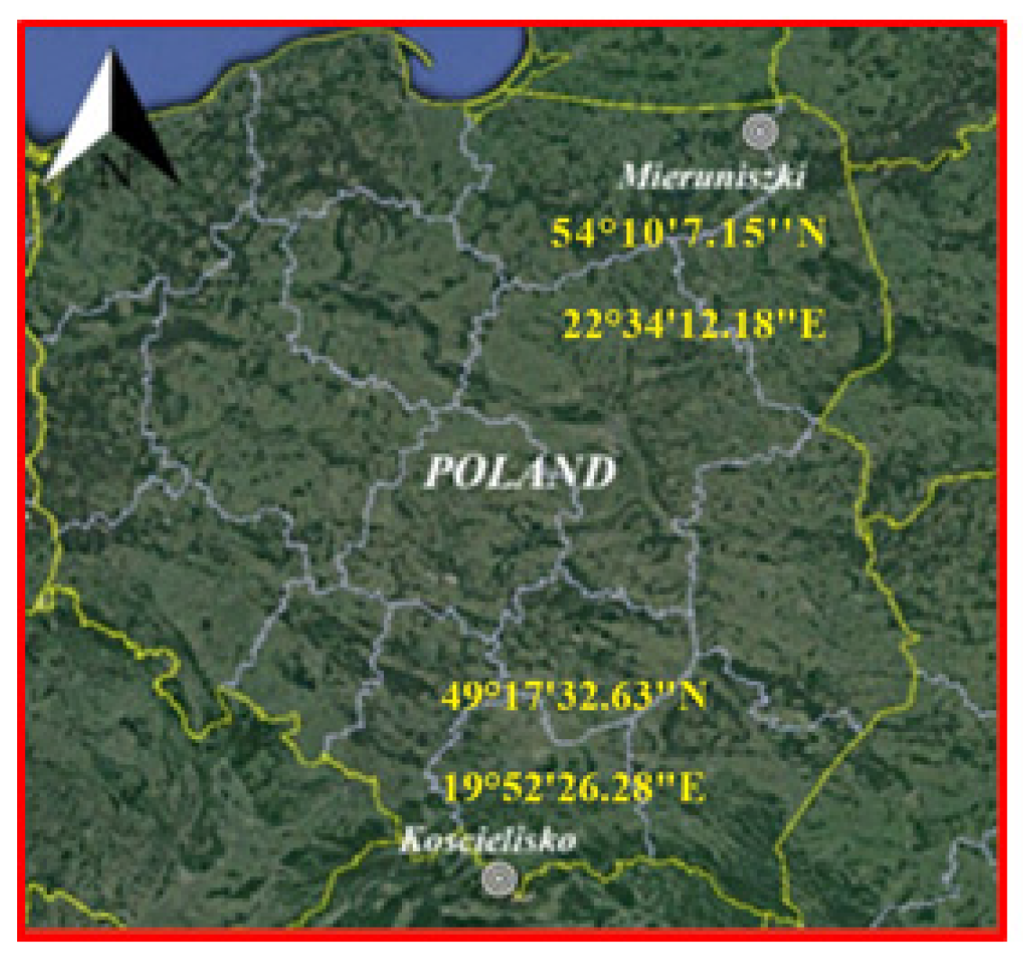
The correction method was designed based on a series of data obtained in the lakeland village of Mieruniszki (54°10′7.15″ N; 22°34′12.18″ E; ASL (Altitude Above Sea Level) 193 m on 13 September 2018. This area is located at the northern end of Poland. It is characterised by high latitude, so the angle of sunlight is lower, the day is shorter and photos acquired in the morning and evening may have worse radiometric quality than photos obtained at the same time, under the same conditions for higher latitudes. The proper selection of test data to assess the correctness of the proposed method was particularly important. The first test set was also acquired in the Mieruniszki area on 22 November 2018. The second set of data was recorded in the mountain village of Kościelisko (49°17′32.63″ N; 19°52′26.28″ E; ASL 941 m) in southern Poland (Figure 1) on 26 September 2018. Kościelisko is located in the south of Poland, and its latitude is about 5° lower. Both regions have their own microclimate. In the Polish mountains during the climatic autumn, strong winds often blow. The most significant impact on the climate is polar air coming from the west, which brings warming and an increase in cloud cover and precipitation on the northern slopes of the mountains during winter. In summer, it causes cooling and an increase in cloud cover. In turn, Mieruniszki is located in the Polish cold pole, where the air temperature is generally lower than in the southern parts of the country. Winds from westerly directions prevail, there are also winds from the south-east. The most windless days fall between July and September. The local microclimate and current atmospheric fronts create the synoptic situation of the region.
Test areas were covered with low grassy vegetation. The occurring buildings in both cases were characterised by a low degree of urbanisation. There are single-family houses, road and technical infrastructure; there are single trees, bushes, grassy vegetation predominates. The test raids in the research areas were carried out on 13 and 26 September and 22 November 2018. In the area of Central and Eastern Europe, it is a period of climatic autumn.
2.2. Data Acquisition
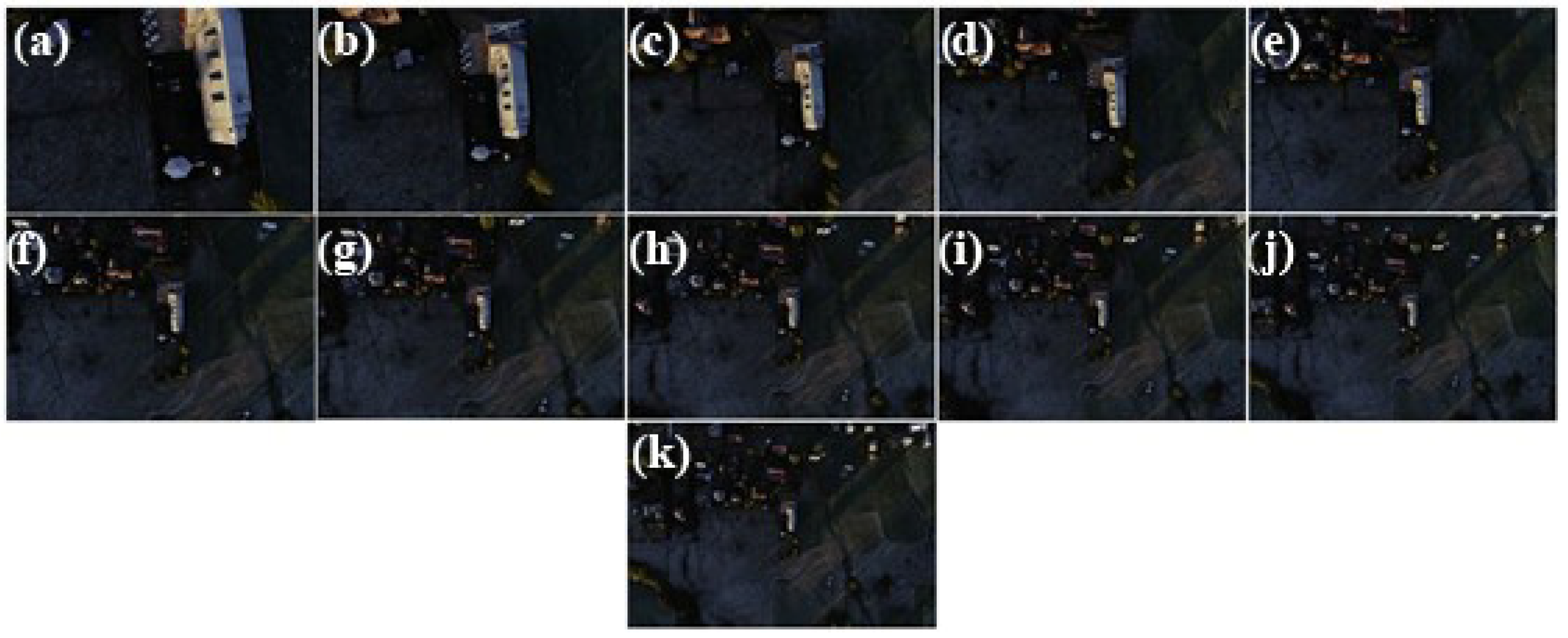
Imagery data in the RGB range were obtained using the DJI Phantom 4 Pro platform (DJI, Shenzhen, China). It is equipped with four electric motors. The platform is equipped with high-resolution digital camera imaging in the visible spectral range. The platform navigation system uses Global Positioning System/Global Navigation Satellite System (GPS/GLONASS) and an optical positioning system as well as two Inertial Measurement Unit (IMU) systems. It is controlled by using an RC controller operating at a frequency of 2.4 GHz. A 1-inch 20-megapixel Complementary Metal-Oxide Semiconductor (CMOS) sensor with a mechanical shutter was installed on the gimbal stabilised in three axes. The focal length of the lens was 24 mm (full-frame). The data were stored in a 24-bit JPG format. Camera sensitivity was set at ISO200 for all images with aperture 4.0 and shutter times ranging between 1/25–1/800. All images were georeferenced with the on-board GPS. Image data were acquired at different flight heights, i.e., in the range from 50 to 300 m (Figure 2.). During the experiment, a total of 646 images with a similar texture (i.e., flat, moderately urbanised areas, arable fields, meadows) were taken.
The meteorological data used to develop parameters for assessing the radiometric quality of images were obtained using the AGAT 20 ground-level measurement station and the SR 10 system for probing the atmosphere. The SR10 system designed for areological measurements allows measuring physical parameters of the atmosphere-air temperature, dew point temperature, humidity, pressure, wind speed and direction, from Earth level to a height of about 30 km, with a measurement frequency of 1 Hz.
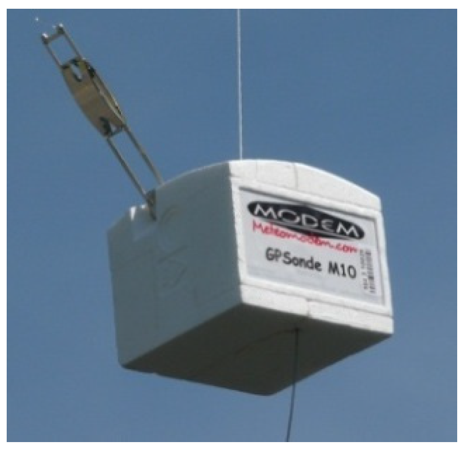
The system consists of the SR10 receiver, M10 radiosondes (Figure 3), ground control kit for radiosonde calibration based on GNSS (12 channels) initialisation. In addition, the system includes an omnidirectional antenna (400MHz), GPS antenna (400MHz) and a tripod. The operating range of the SR10 system is min. 350 km. The receiver works in the 400–406 MHz range.
2.3. Meteorological Conditions
2.3.1. The Synoptic Situation in the Mieruniszki Test Area
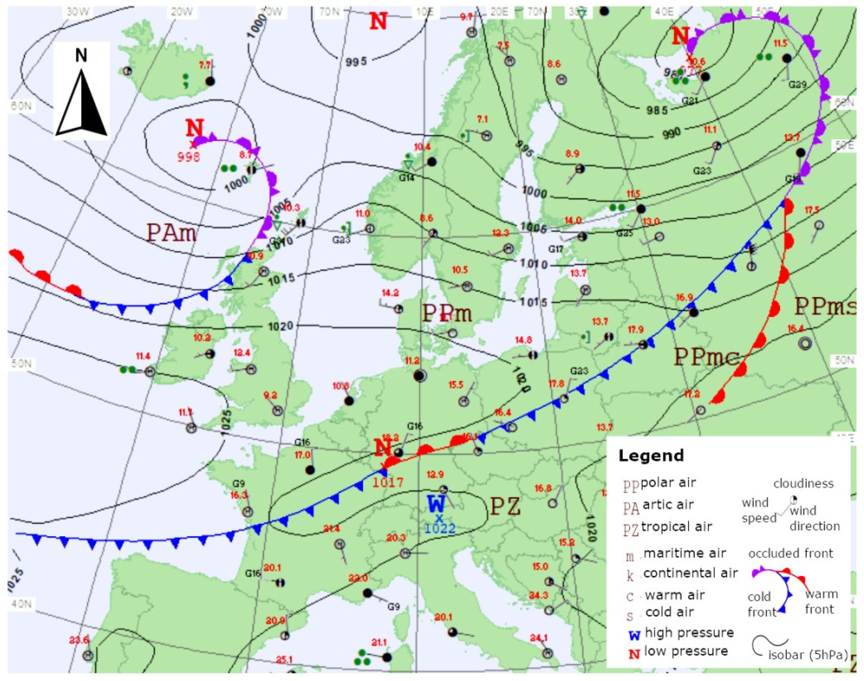
On 13 September 2018, the area of Mieruniszki was under a low-activity cold front associated with a barometric low from northern Scandinavia (Figure 4). A maritime polar air mass flowed over the region from the west, with the velocity of 50–40 km/h and with the stable equilibrium that changed to conditionally unstable as the day passed [38].
At the time of the flights in Mieruniszki, between the hours of 04:00 UTC and 12:00 UTC, the sky coverage was at 8–5/8 Ci, Ac, As, Cu, Sc with the lowest cloud bases at the height of 400–600 m, rising after 07:00 UTC to 600–1000 m. Prevailing wind direction: 250–270°, wind speed: 2–4 kt. Near the end of the considered time interval there were light rain showers. Prevailing visibility was above 10 km, with fog only in the small hours of the morning, limiting the visibility to 6 km. During the flights, the maximum temperature was 15–17 °C. The 0 °C isotherm was located at 3000–2700 m. The humidity ranged from 61.7% to 98.0%.
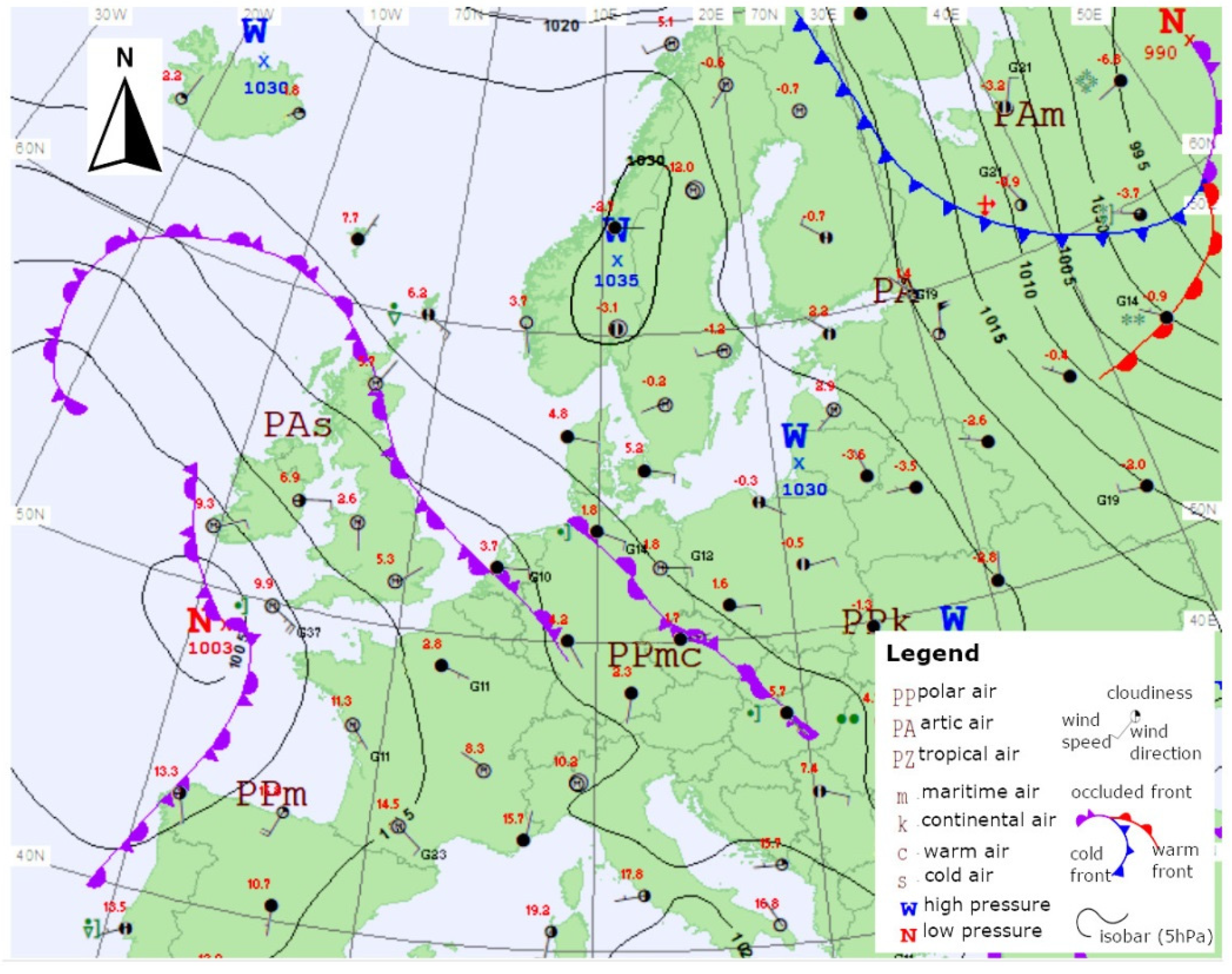
On 22 November 2018, the area of Mieruniszki was in the high-pressure field associated with the barometric high from Kaliningrad (Figure 5). A continental polar air mass flowed over the region from the southwest, with the velocity of 30–20 km/h and with stable equilibrium [38].
During the flights in Mieruniszki, between the hours of 06:00 UTC and 12:00 UTC, the sky coverage was at 6–8/8 with the lowest cloud bases at the height of 300–450 or 600 m. The wind was moderate and changeable (prevalently north-easterly). The prevailing visibility was above 10 km. During the flights, the maximum temperature was −3 °C. The 0 °C isotherm was located at 0 m. Within the range of the clouds, there was light to moderate ice. Various inversions, which had developed after the sunset on the previous evening and during the night, lasted throughout the day, which prevented any changes in the size and height of cloud bases, as well as any increases in temperature. The humidity ranged from 52.2% to 75.2% [38].
2.3.2. The Synoptic Situation in the Kościelisko Test Area
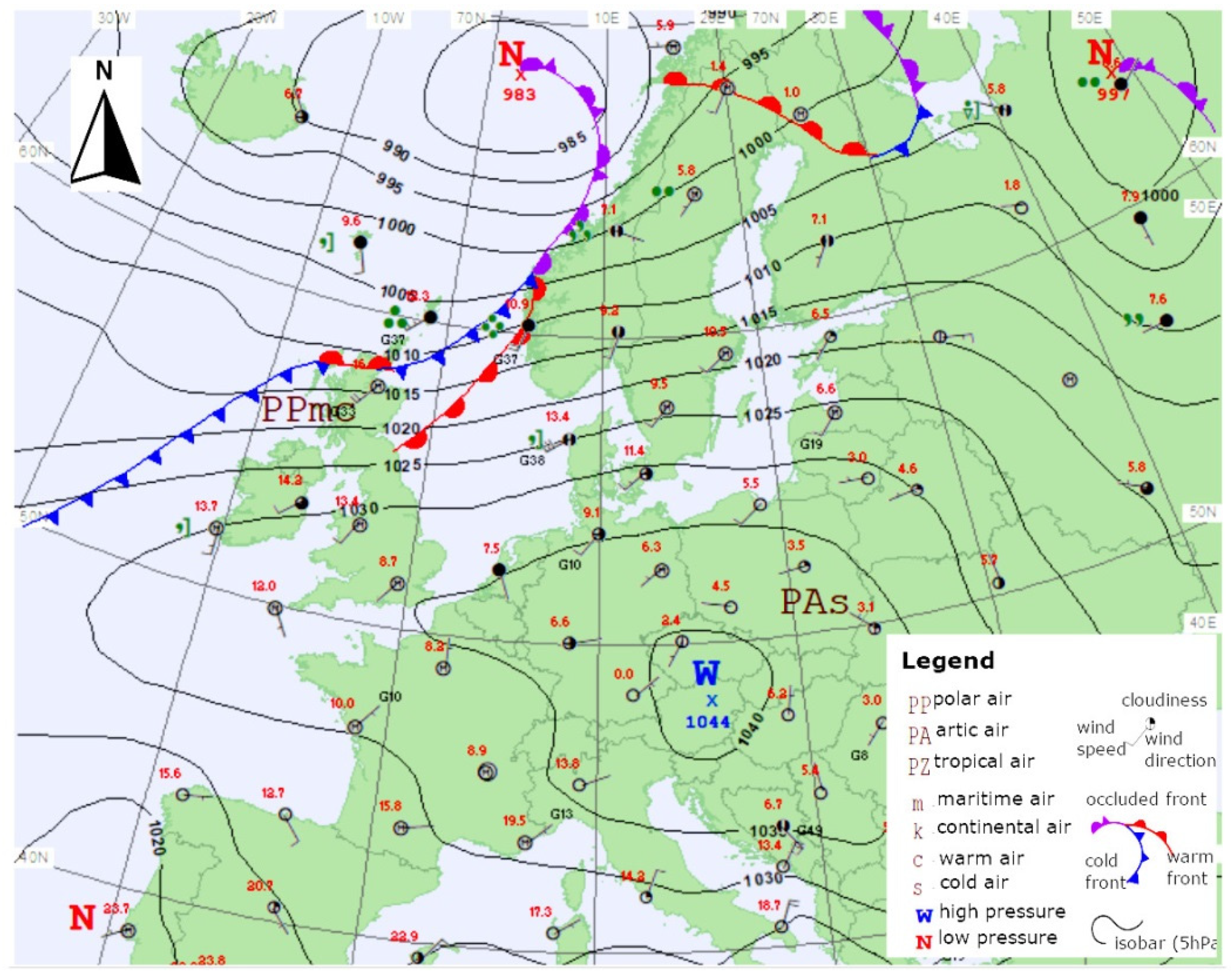
On 26 September 2018, the area of Kościelisko was in the stationary high-pressure field coming in from southern Europe (Figure 6). A maritime polar air mass flowed over the area from the northwest, at the velocity of 50–45 km/h and with a stable equilibrium.
During the flights in Kościelisko between the hours of 07:00 UTC and 17:00 UTC, the sky coverage was at 2–4/8 Ci, Cs, Ac, with lowest cloud bases at the height of 2400–3000 m, with periodic changes to 2–4/8 Cu, Sc, cloud bases at 1800–2400 m. The wind was moderate and changeable, visibility over 10 km. The maximum temperature was 11–13 °C. The 0 °C isotherm was located at 3000–3400 m. The humidity ranged from 40.5% to 83.0% [38].
3. Methodology
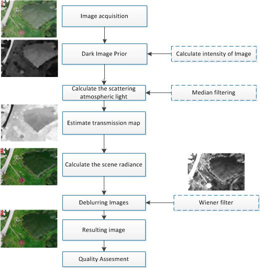
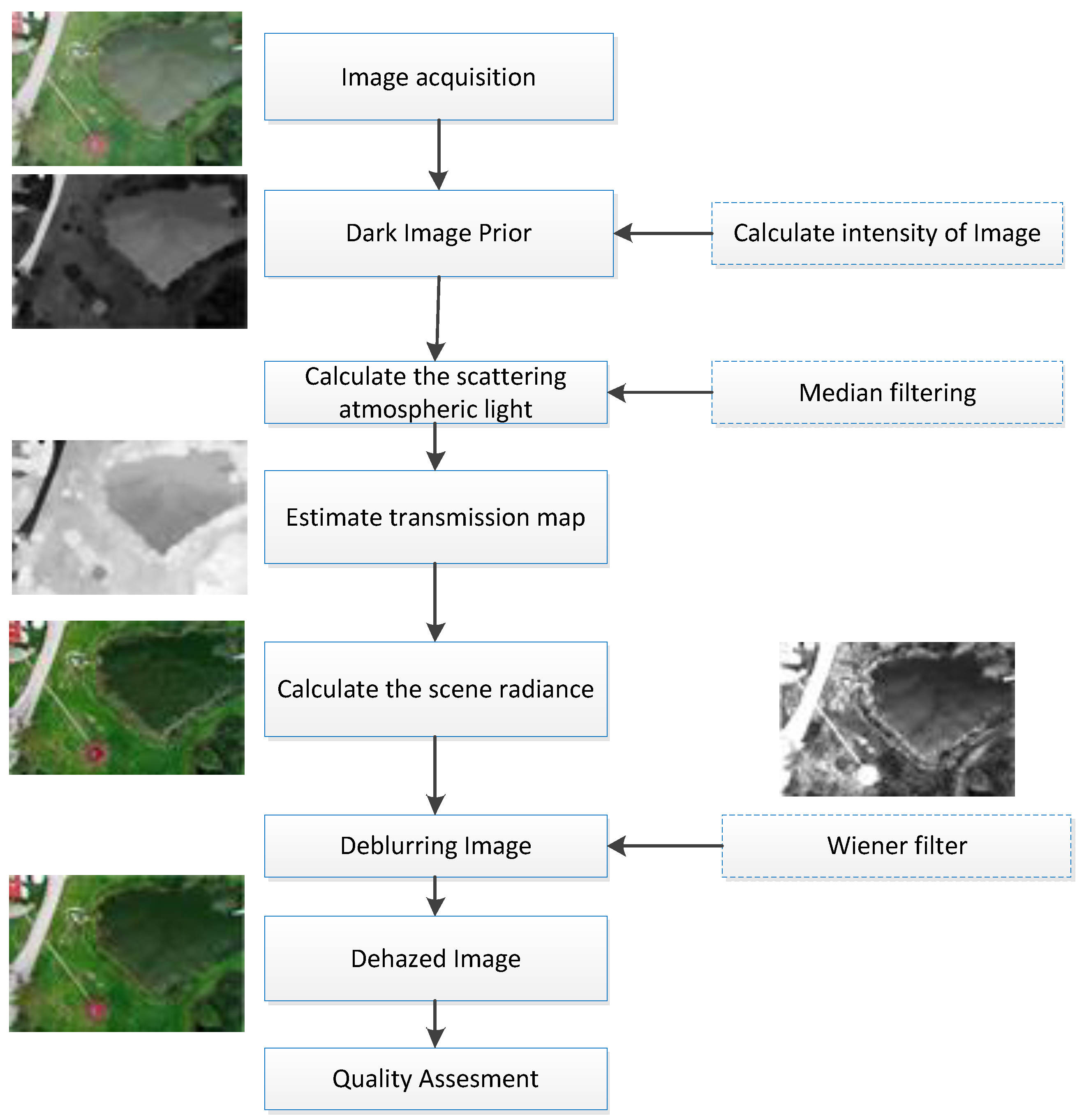
This chapter presents the methods for dehazing images obtained from low altitudes. A block diagram of the overall method workflow is shown in Figure 7.
The following sections present the processing stages (mentioned in the workflow) in detail.
3.1. Dark Image Prior
In the first processing step, Dark Channel Prior (DCP) developed by He et al. [38] was used. Before processing, the intensity value is determined for each image band. The DCP assumes that some fragments of non-fogged images contain at least a few pixels with a low DN value in at least one channel. Based on this, it can be assumed that the dark channel for an excellent radiometric quality image (not covered by haze) tends to 0. Therefore, for each input image, the dark channel could be described by the Equation [29]:
where: is the image band; represents a local patch centred at pixel; minimum operator: performed on each pixel of the image; minimum filter . The minimum number of operators may vary.
3.2. Calculate the Atmospheric Scattering Light
In image processing, the atmosphere dispersion model for adverse weather conditions will have the following form [36]:
The first expression models direct attenuation of the atmosphere, while the second one models the dispersion of light in the air. determines the intensity of image haze, determines the position on the 2D plane: defines the light in the atmosphere, which is treated as a globalconstant and independent of the pixel location. is the reflection coefficient of the object in the image. is the atmospheric attenuation coefficient, and is the distance between the object in the image and the observer, which can be different in each position. It is assumed that in Equation (2) is constant for different wavelengths of the electromagnetic spectrum. This assumption is correct for the case when the particles of the atmosphere are larger (water vapour particles) compared to the wavelength of light. In addition, the value is constant for each part of the image. Transmission t can be expressed as . In turn, atmospheric light can be written as . The simplified Equation (2) will be:
where: is not a hazy image, is the transmission, and is atmospheric light.
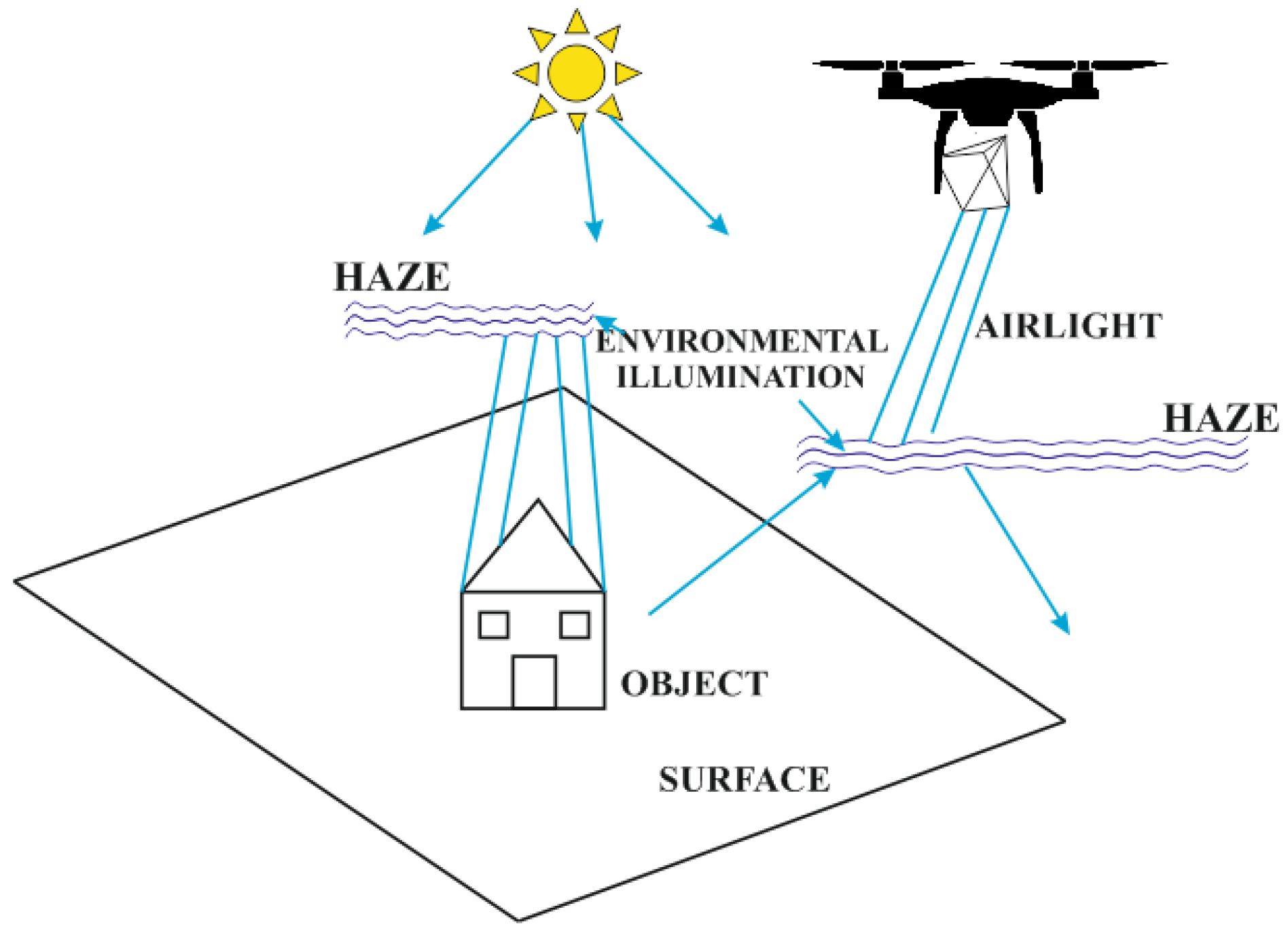
Below (Figure 8) is the optical model of the atmosphere diffusion based on the Lambert reflection model, which is similar to other such models [39].
The model implemented in our methodology is a linear combination of direct radiation transmission and light scattering on water vapour particles in the atmosphere. Direct transmission is the result of the propagation of light in the environment, taking into account the reflectance of objects and attenuation by water vapour particles. Additionally, to preserve the background texture, median filtration with 3 × 3 kernel size was applied [40].
The atmospheric light estimation- will consist of selecting the points with the highest DN considered as the intensity of atmospheric light from the group of pixels. According to the research conducted by He [29], 0.1% of the brightest pixels in the dark channel were selected, and the brightest pixels in the original input image as an estimate of the intensity of atmospheric light.
3.3. Estimating Transmission Map
In the next stage, the atmospheric light determined in the previous step was used to determine the transmission map. In addition, it was assumed that the value of the intensity factor correlates with meteorological measurements of the SR10 system. The value of the Ω coefficient was directly proportional to the humidity intensity during the imagery acquisition and ranged from 0.40 to 0.98. To speed up the calculations, the resolution of the input images has been reduced by half, and the patch size was 15 × 15 pixels. To determine the transmission map, the approach proposed by [29] was used:
- In the first step, Equation (3) was normalised using atmospheric light . After this operation, the Equation is:In this way, it is possible to normalise each R, G, B band of the image independently.
- According to the adopted assumption that is a constant in a local patch (block) and the value is known, the dark channel can be determined by using the min operator [29]:
- In the next step, it is assumed that for the dehazed image (dark channel) , and value is always positive.
- Based on the above, the transmission value for the block (patch) can be determined from the formula:
Whereas the average transmission value is calculated for the whole image.
After the determination of the scattering atmospheric light and transmission map step, the scene radiance was determined based on the Equation:
According to the results [29] the component might be close to zero when the transmission value is also close to zero. As mentioned previously, the proposed methodology will be in the range: .
3.4. Denoising Images
In the next step, in order to reduce the restored image blur and remove noise, an adaptive Wiener filter for the red image channel was used, which uses the statistical estimation of noise parameters for the local neighbourhood of each image point. Filtration was carried out according to the following steps [40]:
- In the first step, the filter kernel size was set empirically to 3 × 3 pixels. The average value and variance were determined for the environment of each pixel of the image according to the following formulas:where is N*M elemental proximity to each point (pixel) of the image.
- In the second step, the square of noise variance is determined for the identified noise waveforms or, in the absence of data, the square of mean-variance from all local neighbourhoods of pixels for the filtered channel (image) is calculated;
Wiener adaptive filter was implemented for the red image band after determining the transmission map. Only the red band was subjected to filtration since the images obtained at high humidity or underexposed have more significant light scattering on larger particles (water vapour particles) (precipitation) from the wavelength (Mie dispersion). After filtering, the red band was combined with the rest of the image.
4. Results and Quality Assessment
In our experiment, the proposed method was implemented by MATLAB R2019a on a PC with Windows 7. Hardware configuration: 2.8 GHz Intel i7 Quad, 8 GB RAM and GeForce graphic card with CUDA technology. Imagery data were obtained at different humidity levels and haze, and during a different time of day with different lighting conditions, during autumn in Central and Eastern Europe (please see Section 2). In total, 646 images were processed.
In addition, a comparative analysis of our method with some of the most popular methods of dehazing images, such as those by: [29], Berman’s et al. [35] and Tarel and Hautiere [36] was conducted. All these methods have also been implemented in the MATLAB environment. For reliable analysis results, the processing parameters for the above techniques are consistent with: [29,35,36]. Table 1 shows the per-image computation time of each algorithm.
Based on Table 1, it can be observed that the shortest processing time was achieved for the Berman’s et al. method and it was 1.75 s, while the longest for the Tarel and Hautiere’s method and it was 2.45 s. It is worth noting, however, that the processing times for individual images are strictly dependent on the number of stages of data processing in a particular algorithm and on the computer’s hardware configuration.
4.1. Quality Assessment
To quantify the quality of images subjected to dehazing operations, commonly used quality assessment indices were used. These indices are based on examining the similarity between the original image before correction and the image after correction. Qualitative indices used in the research presented were calculated for 646 images, and include: root mean square error (RMSE), signal to noise ratio (SNR), peak signal to noise ratio (PSNR), structural similarity (SSIM), which according to [43] assesses the ability to preserve structural information for imagery dehazing methods. Also included is the correlation coefficient (CC), which measures the similarity between two images and the Entropy value original and the Entropy value after dehazing. Entropy determines the complexity of the image texture–the more details visible in the texture, the greater the value this feature takes, the entropy is in the range [0, 8]. The Universal Image Quality Index (Q index) proposed by [43] was also included in the quality assessment. It takes values from 0 to 1. The higher its value, the better the image quality.
4.1.1. Visual Analysis
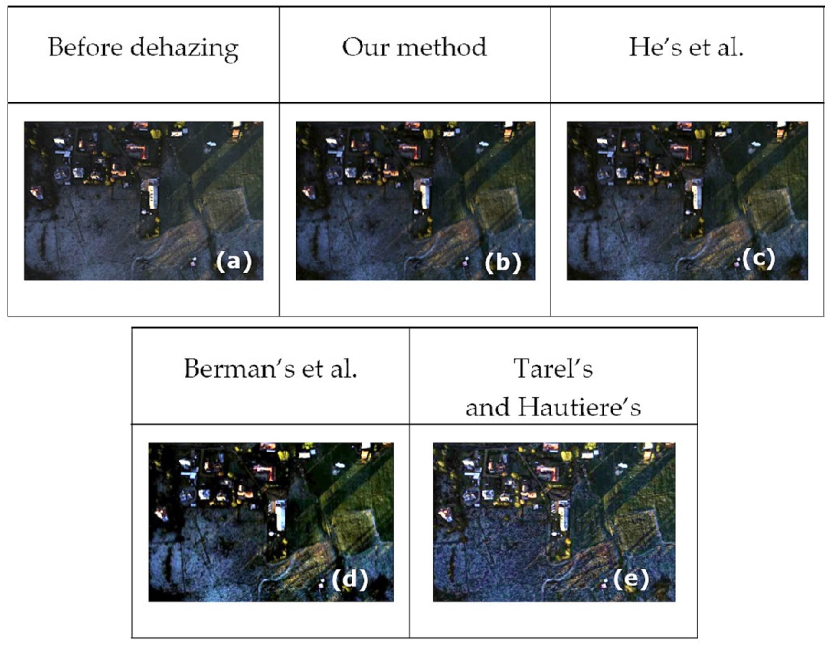
In Figure 9, sample images from the test data set are shown. The visual analysis of these photos shows the results of subsequent processing methods.
Based on the visual analysis (Figure 10, Figure 11 and Figure 12), it can be observed that the application of our method has effectively removed the negative impact of air humidity (haze) on the radiometric quality of images obtained from low altitudes while improving the sharpness of images and their noise reduction.
Application of the basic He’s et al. method an achieved satisfactory results; however, the images are blurred or noisy in some areas.
Moreover, it can be stated that the use of the last two (Berman’s et al. [35] method and Tarel and Hautiere [36]) methods for dehazing introduced colour supersaturation, which may cause the halo effect in images. In addition, in our approach, the use of Wiener filter allowed to remove the blur effect, caused by data acquisition in low light conditions caused by haze.
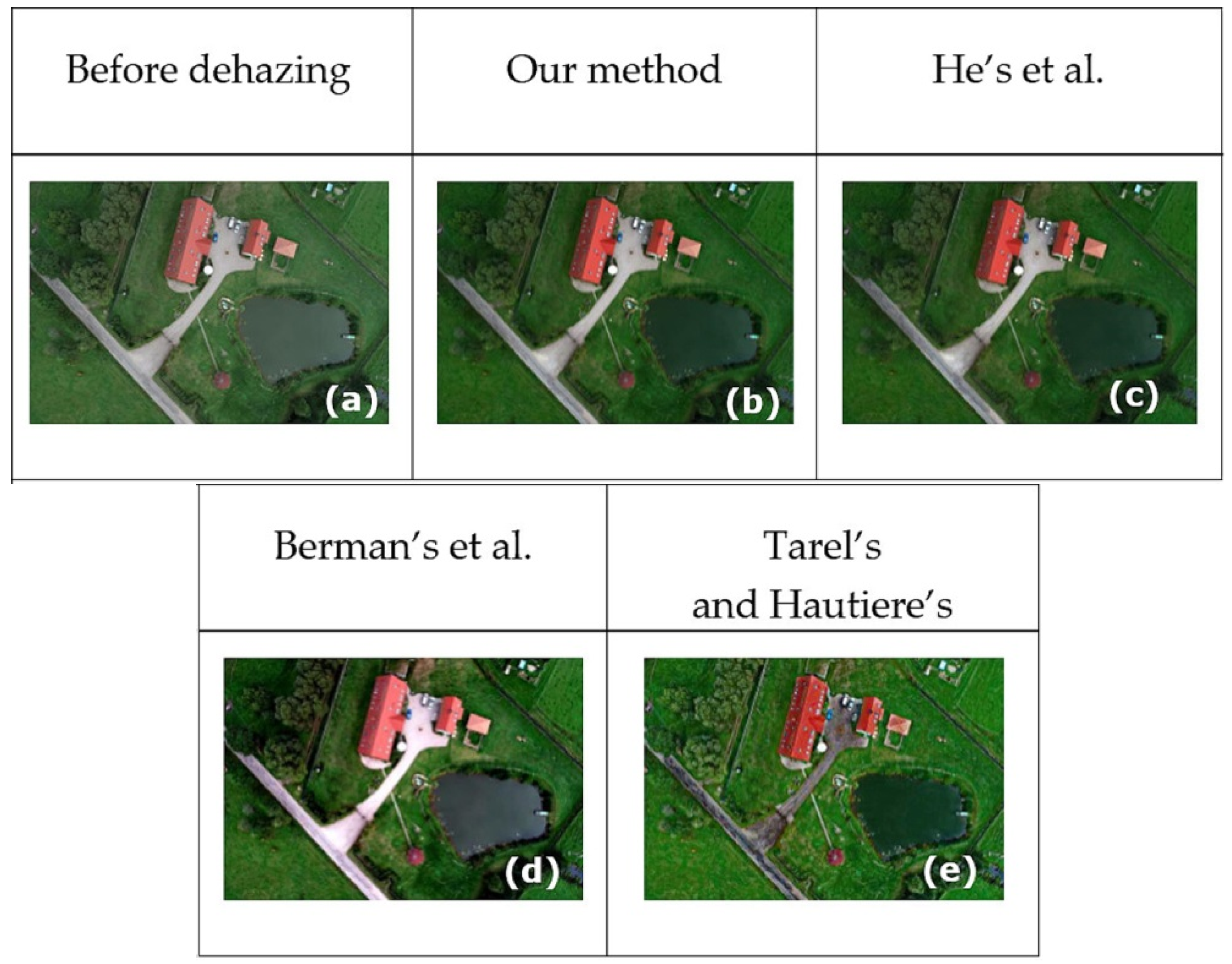
Application of Berman’s et al. method [35] causes images to seem unnaturally overexposed, and the contrast increases too much. An unnatural reproduction of the colour of the water surface and its reflection can be seen on the photographed water reservoir (Figure 10).
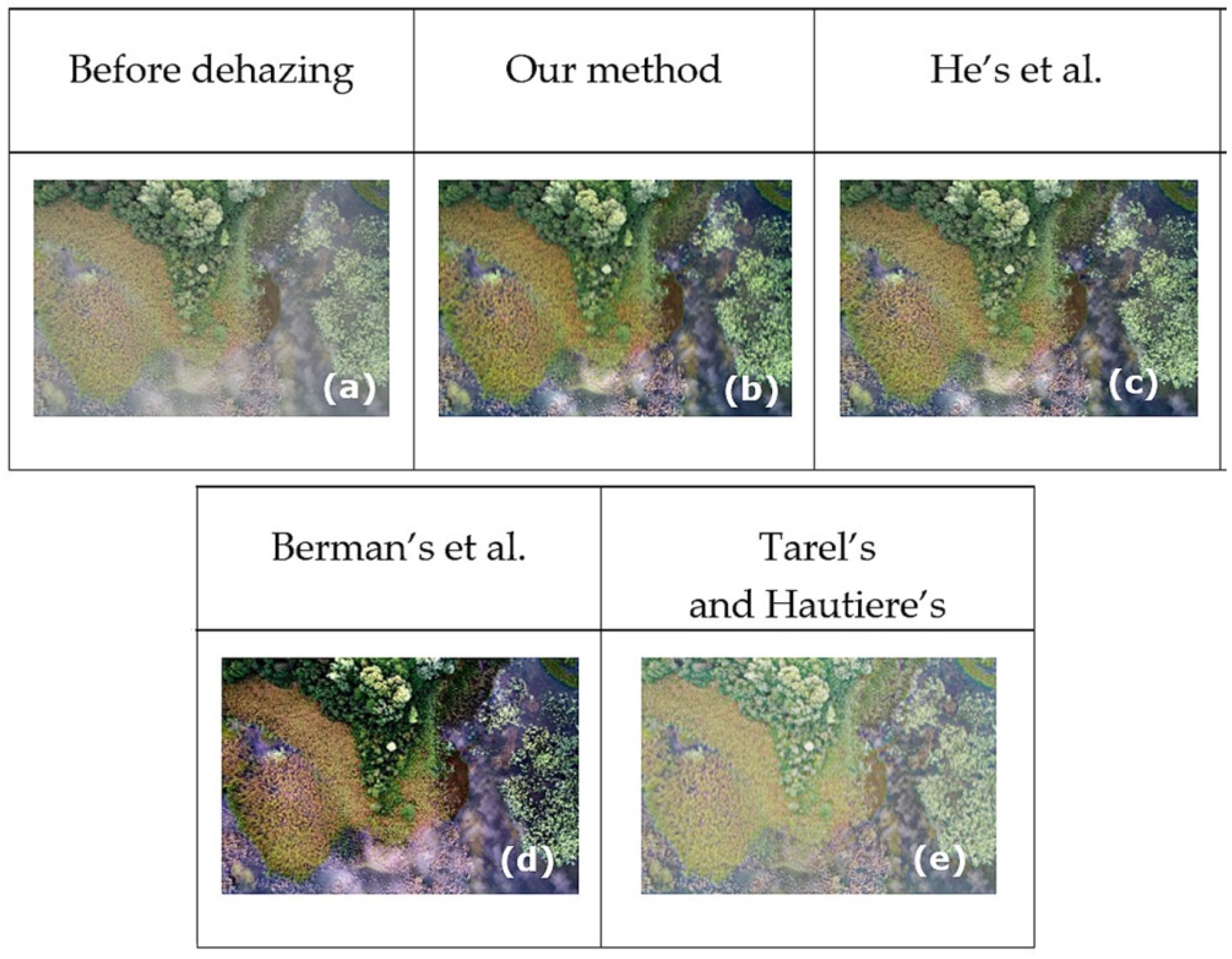
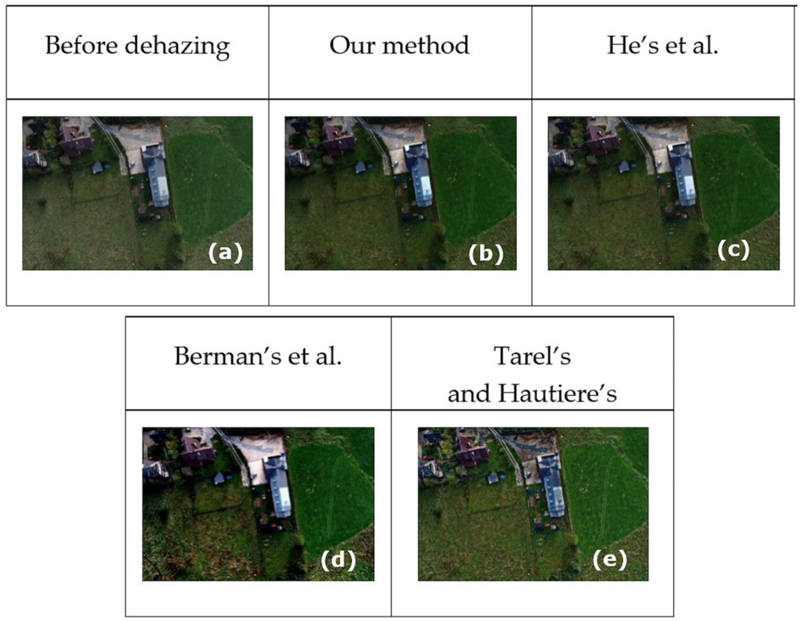
Whereas, based on the analysis of examples of images processed using the Tarel and Hautiere method, [36], it can be seen that these images have been excessively enhanced (Figure 10 and Figure 11). In addition, in this method (Figure 9), very dense fog during the data acquisition caused the negative effect of even more haze after data processing, i.e., the image was even more degraded. That method cannot cope with very dense fog in the image. As shown in Figure 9, method [36] is unable to process a very hazy image. That is because the algorithm incorrectly recognises whether the observed white belongs to the haze or to an object in the scene. As shown above, this algorithm will be unreliable for low altitudes images obtained under dense fog conditions.
Unlike other dehazing methods, our method allows the removal of most of the haze from images and enhances the details of the image, correctly reproduces colours, eliminates excessive gain and possible blur of the image.
4.1.2. Quality Metrics Assessment
PSNR Assessment
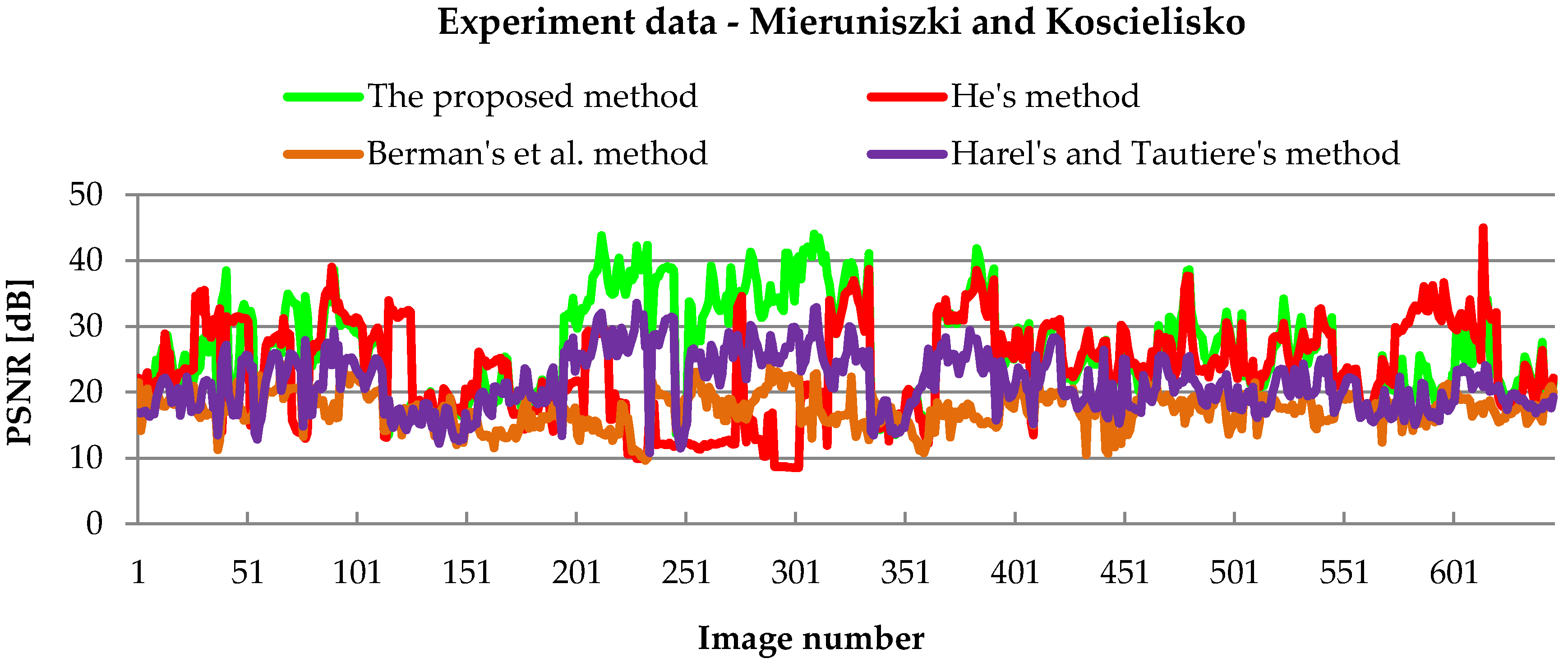
Figure 13 shows the results of comparative analysis for our method and other methods to the PSNR parameter.
Images obtained under good weather conditions are sharp and have a low noise level, which is confirmed by positive and high PSNR values (Table 2). On the other hand, images acquired in impoverished conditions are vague, hazy and noisy, which reflects low index values and negative values.
As known, the higher the PSNR value, the better the image quality. For a sample of 646 images in most cases, the PSNR value for our method is higher than the others. For our approach, the average value was 26.44 [dB]. For He’s et al., the average was 23.57 [dB], for Berman’s et al. method the average was only 17.40 [dB], and for Tarel and Hautiere’s method 21.38 [dB]. Our approach allowed obtaining on average 34% higher values of the PSNR compared to Berman’s et al. method. Whereas, in comparison to the primary method of [29], the results improved by an average of 11%.
Table 2 shows the distribution of PSNR values for reference images obtained from three different flight levels in the early morning, morning and afternoon (test data set of 646 images). The best results are shown in green.
The average values of the PSNR for reference images are from 17.40 to 26.44 [dB], with a standard deviation from 2.60 to 7.41. Maximum values do not exceed 45.01. The minimum value of the ratio is 8.55, and it is the value for the image with the lowest quality in Method [29].
RSME Assessment
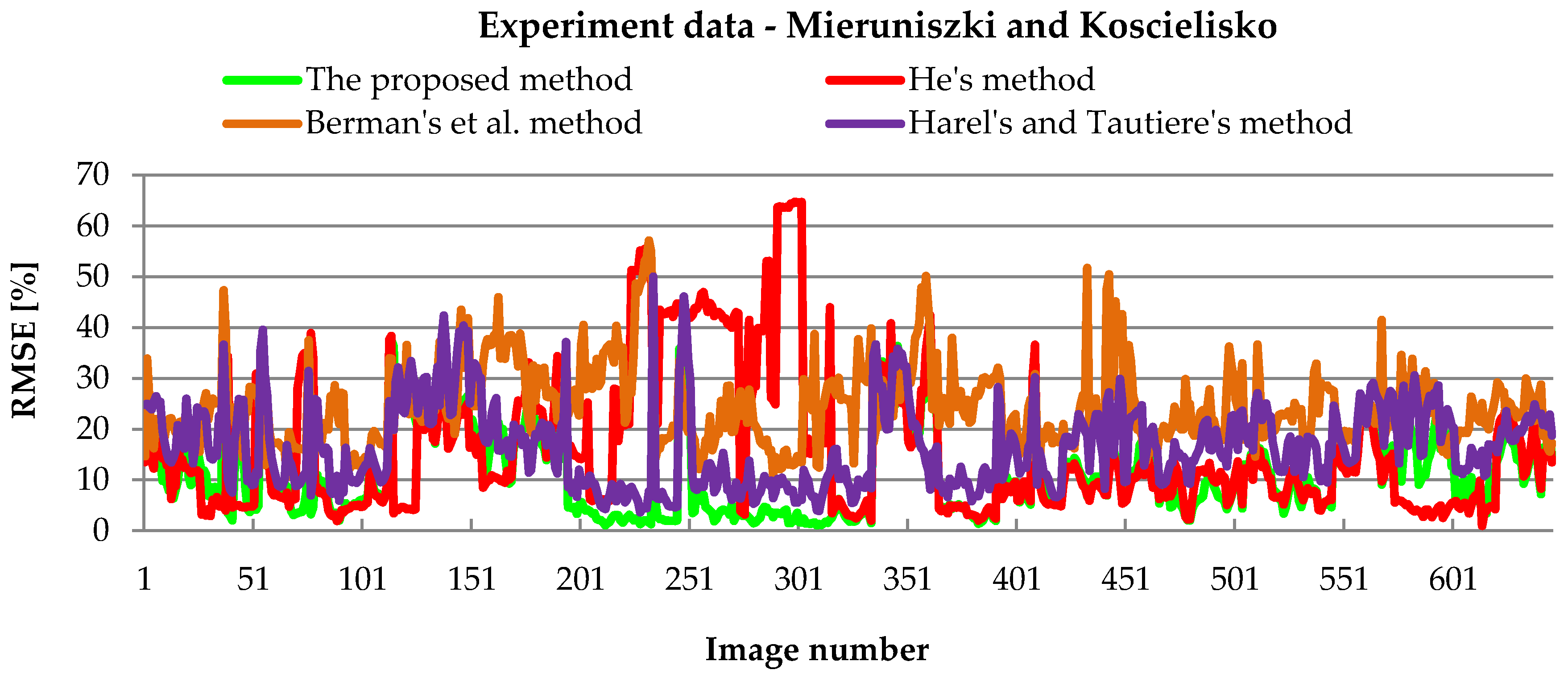
In the literature, many different approaches to assessing image quality can be found. There is no universal procedure. To assess the image quality after data dehazing the mean error values can be used, i.e., RMSE (Root Men Square Error) [355]. The relative RMSE measure is used to avoid large absolute deviations for large values of the DN.
For images from the test data set (Figure 14) for the proposed method, the average RMSE value was equal to 11.4% with a maximum value of 40.5% for one image only. Similarly, for He’s approach, the average RMSE value did not exceed 20% and was equal to 16.1%. In the case of Berman’s et al. method, the average RMSE was 24.5%. For Harel and Tautiere’s method it was 16.7%.
Table 3 shows the distribution of RMSE index values for reference images obtained from three different flight levels in the early morning, morning and afternoon (test data set of 646 images).The best results are shown in green.
Standard deviation values for all considered methods are in the range from 7.7 (Berman’s et al. method) to 8.7% (our approach). Maximum values do not exceed 64.7% (He’s method). The minimum value is 1.1 (Our method and He’s method). The average values of the determined RMSE (Table 3) for test data sets, only for our approach, do not exceed the value of 12% in all spectral bands. This means that the proposed method of images dehazing is highly satisfactory. In addition, it does not degrade its informational content. Additionally, for our approach, obtaining the lowest RMSE value indicates good spectral consistency, i.e., DN value correspondence. Unfortunately, in the case of Berman’s et al. method, the most significant information degradation of images was observed. The differences in the obtained RMSE values for individual test images result from the flight height (from 50 m to 300 m). This is also since as the altitude increases, the atmosphere model changes and the conditions of radiation scattering change. In addition, different humidity at the time of data acquisition and the varied texture of the image should be considered.
SSIM Assessment
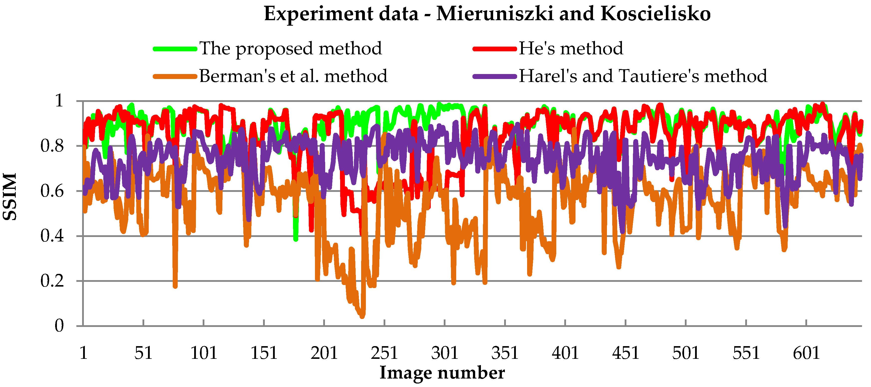
Next, the structural similarity index (SSIM) was applied. This index takes into account three types of image distortion: image luminance, contrast, and structure. For the puposes of the experiment the values 0.01 and 0.03 were adopted for C1 and C2, respectively, and the dynamic range of the image was in the range of 0–255. SSIM is characterised by contrast, brightness and structural similarity of an image. It takes values from 0 to 1. The closer the value is to 1, the better the image quality. The chart below (Figure 15) shows the calculated SSIM values for all test images using specific processing methods. The best results are shown in green.
Based on the chart analysis, it can be seen that the highest SSIM values were obtained for our method and classical He’s method. While the lowest index values were obtained for Berman’s et al. method. The average SSIM value for the proposed method was 0.890, for He’s method 0.843, while the lowest average value was obtained for Berman’s et al. approach and it was 0.564.
Table 4 shows that our approach outperforms the other methods. The best results are shown in green.
Standard deviation values for the considered methods are in the range from 0.071 (our approach) to 0.122 (He’s et al.) [29]. The maximum value obtained was 0.987 (He’s method) [29]. The minimum value is 0.042 (Berman’s et al. method) [35]. Unfortunately, in the case of Berman’s et al. method, the greatest information degradation of images was observed at the expense of their dehazing. Based on the above, it can be concluded that our method obtains the highest SSIM for images from low altitudes in comparison to other existing methods. Therefore, the proposed method balances colours after processing operations but also improves the radiometric quality of images degraded by the adverse effects of the low atmosphere.
Universal Quality Index Assessment
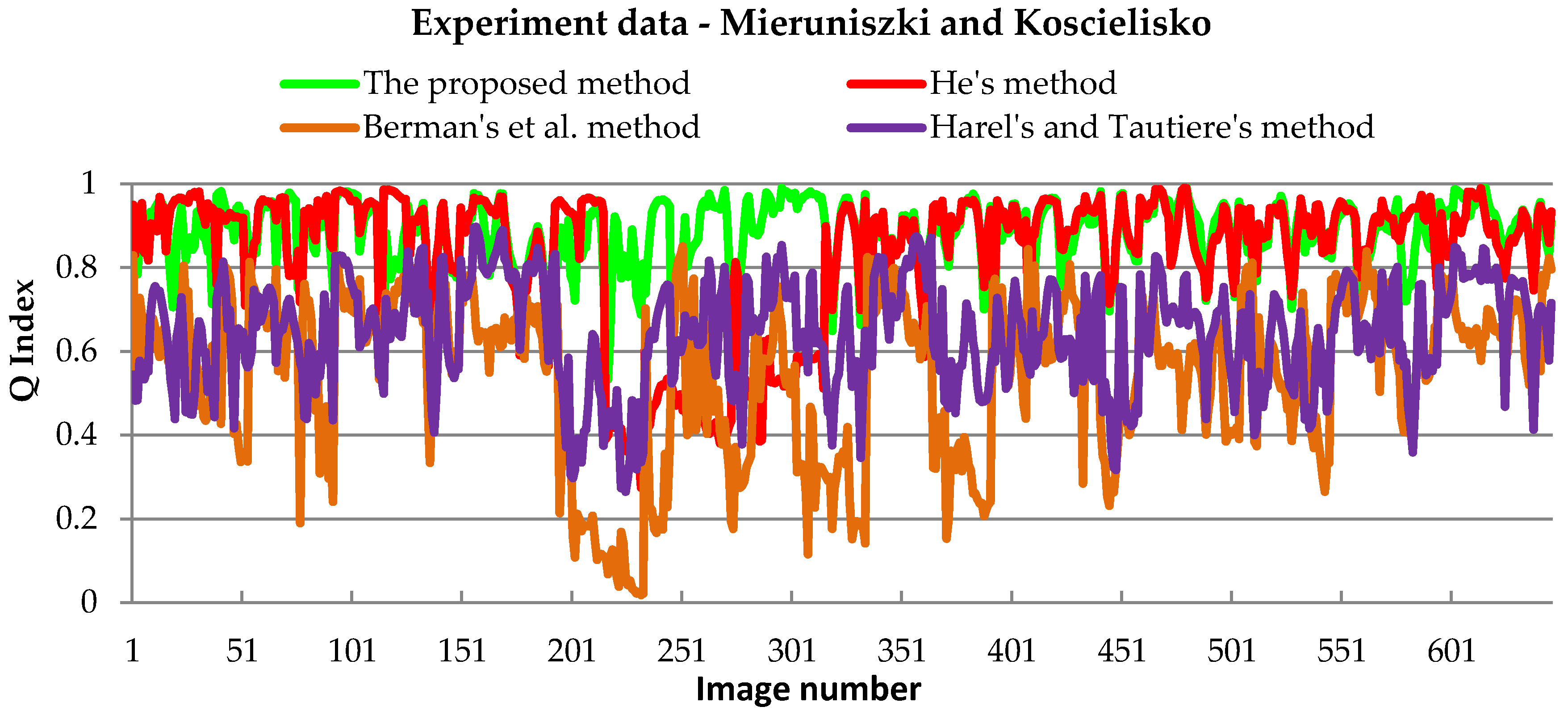
The Q Index was also used in qualitative analyses. This is an image quality evaluation parameter of the full-reference type [43,44]. It takes values from 0 to 1. The closer the value is to 1, the better the image quality. This index was developed to assess image distortion as a combination of three factors: correlation loss, radiometry distortion and contrast distortion. It includes several different statistical parameters characterising the data set—brightness values of pixels in a given image band, and the average value of this index, according to its authors, allows for global assessment of image quality [43]. The following chart (Figure 16) shows the calculated Q index values for all test images using individual processing methods.
Table 5 shows that our approach outperforms the other methods. The best results are shown in green.
Standard deviation values for the considered methods are in the range of 0.081 (our method) to 0.192 (Berman’s et al. approach) [35]. The maximum value obtained was 0.881 (our method). The minimum value is 0.019 (Berman’s et al. method) [35]. In addition, as the results of the previous index (SSIM) analysis have already shown, in the case of Berman’s et al. method, the most considerable information degradation of images was observed at the expense of their dehazing. Analysing the obtained Q index statistical values for individual methods, it can be stated that our method noticeably improved image quality degraded by the negative impact of haze.
Correlation Assessment
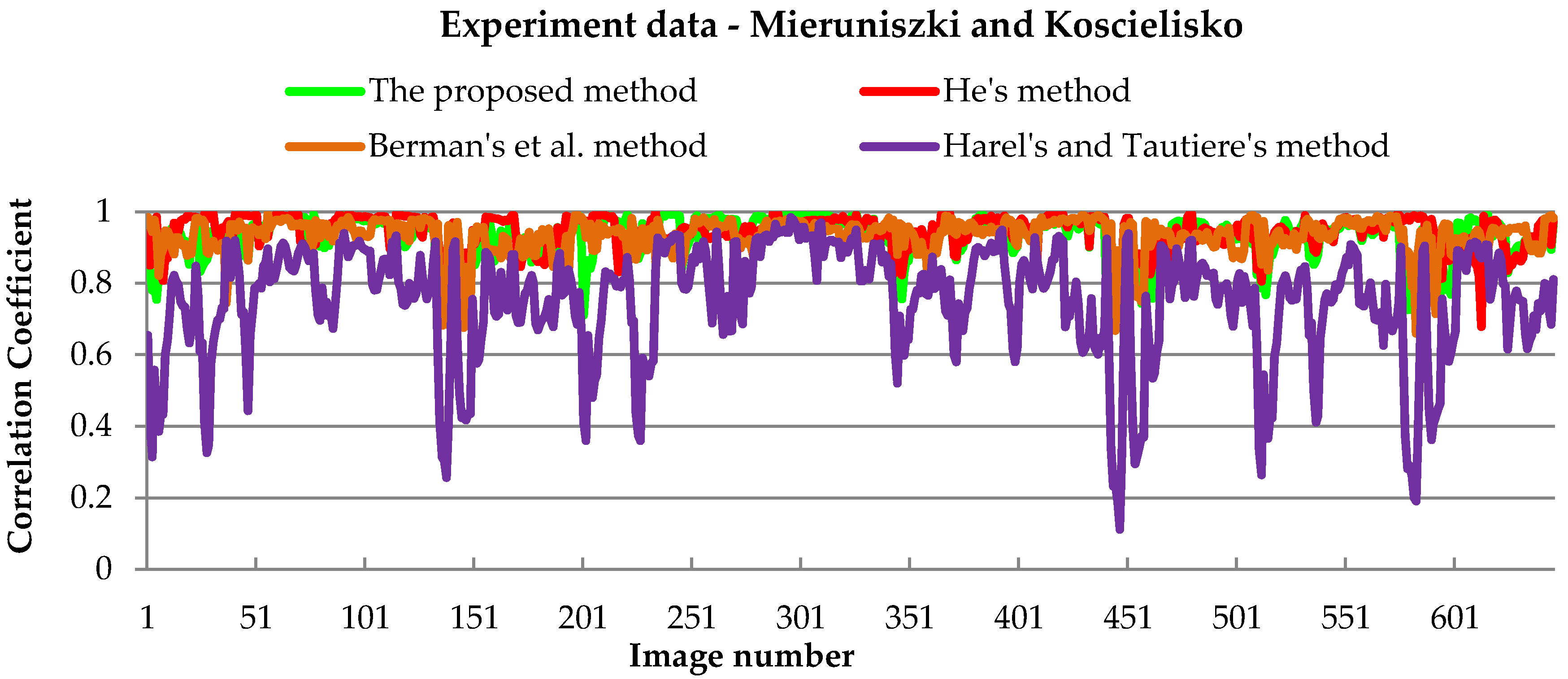
To conduct the comparative analysis, the Correlation Coefficient (CC) between hazy images and dehazed images was also calculated. The CC value depends on the relationship between the covariance of the respective channels of both images and the spread of the pixel values around the mean value in each band of both pictures (standard deviation). That means that for data that retain ideally the same spectral values, i.e., pixel values, the correlation coefficient should be 1. The closer to CC is 0, the less the correlated data are, and therefore the similarity is low [45,46]. The graph below (Figure 17) shows the calculated Cross-Correlation values for all test images using specific processing methods. The best results are shown in green.
Table 6 presents the values of the correlation coefficient between hazy images and dehazed images. The best results are shown in green.
In relation to the correlation values, the average values for the first three methods are about 0.93. After radiometric correction, correlation values are close to 1; it means that the global image statistics have not changed, while the absolute radiometric quality of the image radiometric has improved. Only when processing using the Harel and Tautiere’s method, the average correlation was 0.751, and also for this method the lowest correlation coefficient value was obtained, it was only 0.112, which means quite a significant degradation of the spectral information in the image. In turn, the results for our methods are very similar to [29].
Entropy Compare Analysis
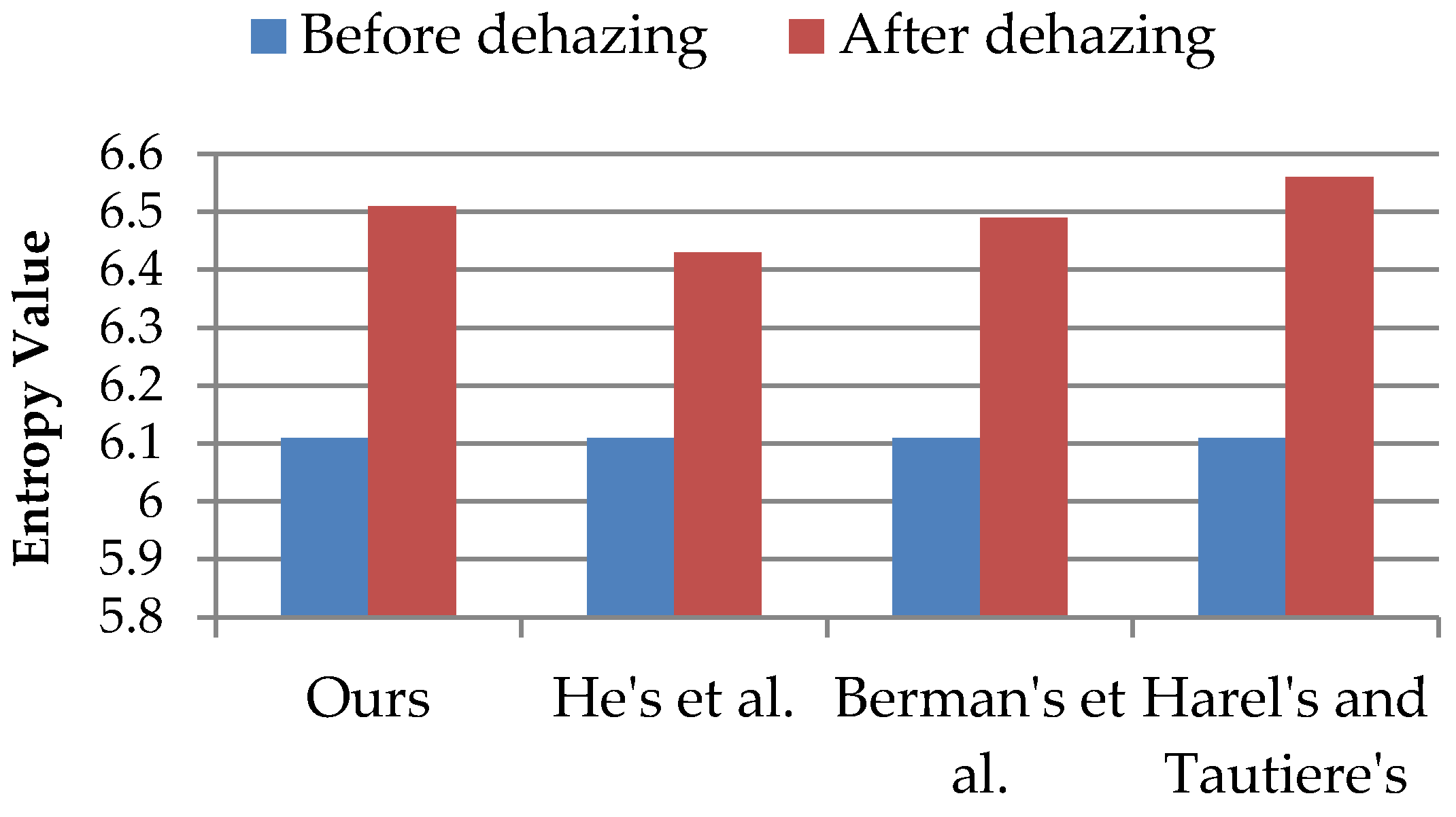
The last verification factor for image quality assessment was determining the entropy value (Figure 18) for images before and after processing. As mentioned before, the more details are visible in the texture, the higher value this feature has, the entropy is in the range [0, 8].
The average Entropy value for the original test images was 6.11. As a result of the implementation of our approach, the average entropy value increased to 6.51, i.e., by 7%. That indicates an improvement in the quality of images, especially concerning increasing the information capacity of the texture. While, for He’s et al. the average value was 6.43, for Berman’s et al. 6.49, while for Tarel’s and Hautiere’s the highest value was obtained for all methods—6.56. If the analyses on previous qualitative indices were not carried out, it could be erroneously concluded that the last method is the best, which in global terms of quality assessment, assessing only increasing the detail of the texture is not objective. In turn, in all cases, the implementation of specific methods allowed the noticeable increase of the amount of information visible in the image texture.
A Statistical Significance Test of Results
Wilcoxon’s signed-rank test was used to determine the statistical significance of the results [47]. Such approach allowed to determine if the differences between the compared methods are really significant. For this work, the p-value was used to indicate the equality of the two comparison methods—Our method with other tested methods, at a p = 0.05 level significance. The test verifies the hypothesis: H0: there are no differences between measurements; H1: there are statistically significant differences between the measurements.
Table 7 presents the tests for each pair of two methods, ours and another tested method. The presented results show that the method we proposed significantly differs from the others in the field of dehazing images. The smallest differences occurred between our method, and He’s et al. Method; p-value is equal to <0.0001 and 0.048 for CC and RMSE, respectively. Also, z-score generally have the lowest values for all compared pairs. Based on the statistical significance test, the relatively highest convergence of results is associated with similar processing steps proposed by He et al. [29]. In turn, the most significant differences are between our method and Tarel and Hautiere’s method, where p-values are very low, and z-score (except for PSNR) are lower than −5. Nevertheless, all z-score values for each pair present differences in methods and emphasise the real significance of our approach. The exception is p-value equal to 0.379 for CC for comparison of Our method with Berman’s et al. That shows that for this case there is no basis for rejecting the H0 hypothesis and in some cases differences in the results for these two methods may be insignificant. However, in all other cases, p-values are lower than 0.05, so the differences between the compared methods are really significant.
5. Discussion
In this paper, a novel method of dehazing images obtained from low altitude was proposed. Unlike most existing solutions, we address this problem for images obtained from low altitudes, taking into account the low atmosphere influence. The algorithms used so far were dedicated to satellite imagery or high-altitude aerial imagery. On the other hand, other methods of dehazing images commonly used in digital image processing degraded the image information content, as demonstrated by the analysis of qualitative indices values. Our correction method is based on the Dark Channel Prior model, which was proposed by [29]. Our solution allows for the removal of haze from images obtained from low altitudes. As proven, based on the proposed data set, our method is useful for images acquired at the height from 50 to 300m with relative humidity (fog) in the range from 40% to 99%. The experiments performed confirmed the impact of air humidity (in particular radiation mists) on the quality of images obtained from low altitudes. In addition, our method allows for the removal of the adverse effects of noise and blur of the image while maintaining its detail thanks to the use of an adaptive Wiener filter. Image colours and contrast remain realistic and physically correct, which, unfortunately, is not provided by popular dehazing methods, such as the Tarel and Hautiere method considered in analyses, [36].
The obtained test results prove the universality of the presented approach for different heights and different lighting conditions and air humidity. The presented research shows the validity of processing images to remove the negative impact of haze. The experiments performed also indicate a new direction of research to develop new models of radiometric correction of images, which will be dedicated only to images obtained from UAVs.
The proposed correction method will reduce radiometric differences in the images contained in the block due to the influence of haze (fog) and the negative impact of air humidity.
In relation to the comparative analyses, our method successfully removed the haze from the image in the vast majority of cases. Regarding the original method proposed by [29], the results for the PSNR index improved by an average of 11%. In turn, in the case of comparative analysis to the Tarel and Hautiere’s method [36] from some images, the haze has been adequately removed, while others have been degraded, making them useless in the context of further analyses. It can be stated that our method and [29] gave the best results in removing haze, while colours and pixel values were preserved. Analysing the values of individual qualitative indices, it can be clearly seen that our method works best, taking into account both qualitative and quantitative assessment and excellent visual quality of the images. Concerning one of the more essential indicator, PSNR (Table 2), for our method, the average value of this index was 26.44 [dB], while the worst result was obtained for Berman’s et al. and it was 52% worse than the proposed solution. Similar results were obtained as a result of research carried out by [48]. In their work, the authors proposed an image dehazing method based on feature learning. For the preformed method, PSNR values for test data ranged from 16.90 [dB] to 21.93 [dB].
When analysing the RMSE results [%] our method also gave the best results, the average RMSE error value was only 11.4%. However, once again, while verifying the processing results with this index, Berman’s et al. method [35] proved to be the least effective, the average value was RSME 24.5%. The results of this indicator mean that the processing method used degrades the information content of the image.
Also, analysis of the results from Table 4 confirms the effectiveness of the proposed method, where the average value of the SSIM index for our approach was 0.890, and the worst average value was obtained for Berman’s et al. method [35], and it was 0.564.
As demonstrated in the calculated correlation values for our method, the average correlation value is 0.930 (Table 6). On this basis, it can be concluded that the global statistics of images have not changed, and only its absolute radiometric quality has been improved. The proposed strategy showed better results compared to similar methods. An improvement of even a few percent is significant because it will bring the spectral properties of objects in the image closer, as well as improving the interpretation properties of such images.
In turn, by performing visual analysis based on the example of Figure 10b it can be observed that sometimes water reservoirs after dehazing become too dark because too much atmospheric light is removed from them; DN values are too low. On the transmission map they are marked as very dense haze and algorithms based on dark channel prior try to remove them. That subtracts an incorrect value in these regions and makes the image on which the water was photographed too dark. One solution to this problem may be to mask these areas and not apply the algorithm on them.
The limitation of the proposed method, as well as other similar algorithms based on the statistical values of the image, is that it may not work on some specific examples of images, e.g., obtained in very bad weather conditions. When a strong fog obscures only part of the object photographed in the image, the use of the algorithm will distort colour reproduction in the image, and as a consequence degrade the spectral quality of the image. The use of radiometric correction that includes the impact of the low atmosphere is crucial to ensure the accuracy of subsequent analyses related to remote sensing from low altitudes; therefore, it is recommended to use calibration panels with a known reflection coefficient to verify data calibration and estimate the radiometric error in each processed image.
Furthermore, the limitation of the proposed method does not take into account geophysical variables such as soil moisture. In order to overcome this limitation, future research will focus on modifying the proposed solution by taking into account several factors, i.e., land cover, water quality, soil moisture and also season.
6. Conclusions
The paper presents the results of research on methods of dehazing images acquired from low altitudes. To remove the haze caused by the negative influence of the low atmosphere on images obtained from UAVs, the Dark Channel Prior algorithm along with the Wiener adaptive filter, were applied. The parameters used in our method have been determined empirically. Our approach is dedicated to images obtained from a low altitude, especially for the most commonly used heights in UAV remote sensing, i.e., from 50 to 300 m. We evaluated the effectiveness of the proposed method using many qualitative indicators. The results of our experiments confirmed the effectiveness of our methods in comparison with several other popular methods used for dehazing images. In addition, thanks to test imagery data sets obtained at different heights and under different atmospheric conditions, we have demonstrated the range of effectiveness of our methods, which is extremely important in improving the quality of images obtained in various conditions.
In our future research work we would adapt our methodology to data acquired with high spatial resolution sensors. Moreover, further research would be focused on the improvement of presented solutions, primarily of automatic parameters preselection for different acquisition heights and water vapour content. Additionally, we plan to add more case studies with a more specific focus on different geophysical variables.
Author Contributions
All authors contributed to the experimental design and participated in the collection of UAV data. All authors provided editorial advice and participated in the review process. Conceptualisation, M.K.; methodology, D.W.; data analysis A.S. They also interpreted the results and wrote the paper; data acquisition M.K and D.W. All authors have read and agreed to the published version of the manuscript.
Funding
This research is funded by the Ministry of National Defence Republic of Poland, Grant No. GB/1/2018/205/2018/DA-990.
Acknowledgments
This paper has been supported by the Military University of Technology, the Faculty of Civil Engineering and Geodesy, Institute of Geospatial Engineering and Geodesy.
Conflicts of Interest
The authors declare no conflict of interest.
References
- Dalla Mura, M.; Benediktsson, J.A.; Waske, B.; Bruzzone, L. Morphological attribute profiles for the analysis of very high resolution images. IEEE Trans. Geosci. Remote Sens. 2010, 48, 3747–3762. [Google Scholar] [CrossRef]
- Woloszyn, E. An Overview of Meteorology and Climatology; Gdansk University of Technology: Gdańsk, Poland, 2009; p. 26. ISBN 978-83-7775-237-1. [Google Scholar]
- Mazur, A.; Kacprzak, M.; Kubiak, K.; Kotlarz, J.; Skocki, K. The influence of atmospheric light scattering on reflectance measurements during photogrammetric survey flights at low altitudes over forest areas. Leśne Prace Badawcze 2018, 79. [Google Scholar] [CrossRef] [Green Version]
- Shao, S.; Guo, Y.; Zhang, Z.; Yuan, H. Single Remote Sensing Multispectral Image Dehazing Based on a Learning Framework. Math. Probl. Eng. 2019. [Google Scholar] [CrossRef]
- Chavez, P.S. Atmospheric, solar, and M.T.F. corrections for ERTS digital imagery. Proc. Am. Soc. Photogramm. 1975, 69, 459–479. [Google Scholar]
- Chavez, P.S., Jr. An Improved Dark-Object Subtraction Technique for Atmospheric Scattering Correction of Multispectral Data. Remote Sens. Environ. 1988, 24, 459–479. [Google Scholar] [CrossRef]
- Zarco-Tejada, P.J.; Morales, A.; Testi, L.; Villalobos, F.J. Spatio-temporal patterns of chlorophyll fluorescence and physiological and structural indices acquired from hyperspectral imagery as compared with carbon fluxes measured with eddy covariance. Remote Sens. Environ. 2013, 133, 102–115. [Google Scholar] [CrossRef]
- Huang, Y.; Ding, W.; Li, H. Haze removal for UAV reconnaissance images using layered scattering model. Chin. J. Aeronaut. 2016, 29, 502–511. [Google Scholar] [CrossRef] [Green Version]
- Tagle Casapia, M.X. Study of Radiometric Variations in Unmanned Aerial Vehicle Remote Sensing Imagery for Vegetation Mapping. Master’s Thesis, Lund University, Lund, Sweden, 2017. [Google Scholar]
- Richter, R. A spatially-adaptive fast atmospheric correction algorithm. Int. J.Remote Sens. 1996, 17, 1201–1214. [Google Scholar] [CrossRef]
- Richter, R. Atmospheric correction of DAIS hyperspectral image data. Comput. Geosci. 1996, 22, 785–793. [Google Scholar] [CrossRef]
- Osińska-Skotak, K. Wpływ korekcji atmosferycznej na wyniki cyfrowej klasyfikacji. Acta Sciennarum Polonorum Geodesia et Descriptio Terrarum 2005, 4, 41–53. [Google Scholar]
- Jakomulska, A.; Sobczak, M. Radiometric correction of satellite images—Methodology and exemplification. Teledetekcja Srodowiska 2001, 32, 152–171. [Google Scholar]
- Jones, S.; Reinke, K. (Eds.) Innovations in Remote Sensing and Photogrammetry; Springer Science & Business Media: Berlin, Germany, 2009. [Google Scholar]
- Richards, J.A. Remote Sensing Digital Image Analysis; Springer: Berlin, Germany, 2006; p. 437. [Google Scholar]
- Osinska-Skotak, K. The importance of radiometric correction in satellite images processing. Arch. Photogramm. Cartogr. Remote Sens. 2007, 17, 577–590. [Google Scholar]
- Gao, B.C.; Heidebrecht, K.B.; Goetz, A.F. Derivation of scaled surface reflectances from AVIRIS data. Remote Sens. Environ. 1993, 44, 165–178. [Google Scholar] [CrossRef]
- Qu, Z.; Kindel, B.; Goetz, A.F.H. The High Accuracy Atmospheric Correction for Hyperspectral Data (HATCH) model. IEEE Trans. Geosci. Remote Sens. 2003, 41, 1223–1231. [Google Scholar]
- Matthew, M.; Adler-Golden, S.; Berk, A.; Felde, G.; Anderson, G.; Gorodetzky, D.; Paswaters, S.; Shippert, M. Atmospheric Correction of Spectral Imagery: Evaluation of the FLAASH Algorithm with AVIRIS Data. In Proceedings of the 31st Applied Imagery Pattern Recognition Workshop, Washington, DC, USA, 16–18 October 2002; pp. 157–163. [Google Scholar]
- Black, M.; Fleming, A.; Riley, T.; Ferrier, G.; Fretwell, P.; McFee, J.; Achal, S.; Diaz, A.U. On the atmospheric correction of Antarctic airborne hyperspectral data. Remote Sens. 2014, 6, 4498–4514. [Google Scholar] [CrossRef] [Green Version]
- Berk, A.; Anderson, G.P.; Acharya, P.K.; Bernstein, L.S.; Muratov, L.; Lee, J.; Fox, M.J.; Adler- Golden, S.M.; Chetwynd, J.H.; Hoke, M.L.; et al. MODTRAN5: A reformulated atmospheric band model with auxiliary species and practical multiple scattering options. Proc. SPIE 2005. [Google Scholar] [CrossRef]
- Głowienka, E. Comparison of atmospheric correction methods for hyperspectral sensor data. Arch. Photogramm. Cartogr. Remote Sens. 2008, 18a, 121–130. [Google Scholar]
- Makarau, A.; Richter, R.; Muller, R.; Reinartz, P. Haze detection and removal in remotely sensed multispectral imagery. IEEE Trans. Geosci. Remote Sens. 2014, 52, 5895–5905. [Google Scholar] [CrossRef] [Green Version]
- Zhang, Y.; Guindon, B.; Cihlar, J. An image transform to characterize and compensate for spatial variations in thin cloud contamination of Landsat images. Remote Sens. Environ. 2002, 82, 173–187. [Google Scholar] [CrossRef]
- Seow, M.J.; Asari, V.K. Ratio rule and homomorphic filter forenhancement of digital colour image. Neurocomputing 2006, 69, 954–958. [Google Scholar] [CrossRef]
- Kedzierski, M.; Wierzbicki, D. Methodology of improvement of radiometric quality of images acquired from low altitudes. Measurement 2016, 92, 70–78. [Google Scholar] [CrossRef]
- Zhou, J.; Zhou, F. Single image dehazing motivated by Retinex theory. In Proceedings of the 2013 2nd International Symposium on Instrumentation and Measurement, Sensor Network and Automation (IMSNA), Toronto, ON, Canada, 23–24 December 2013; pp. 243–247. [Google Scholar]
- Wang, W.; Guan, W.; Li, Q.; Qi, M. Multiscale single image dehazing based on adaptive wavelet fusion. Math. Probl. Eng. 2015, 2015, 131082. [Google Scholar] [CrossRef] [Green Version]
- He, K.; Sun, J.; Tang, X. Single image haze removal using dark channel prior. In Proceedings of the IEEE Conference on Computer Vision and Pattern Recognition, Miami, FL, USA, 20–26 June 2009; pp. 1956–1963. [Google Scholar]
- Xie, B.; Guo, F.; Cai, Z. Universal strategy for surveillance video defogging. Opt. Eng. 2012, 51, 1–7. [Google Scholar] [CrossRef]
- Park, D.; Han, D.; Ko, H. Single image haze removal with WLS-based edge-preserving smoothing filter. In Proceedings of the IEEE International Conference on Acoustics, Speech, and Signal Processing, Vancouver, BC, Canada, 26–31 May 2013; pp. 2469–2473. [Google Scholar]
- Tan, R.T. Visibility in bad weather from a single image. In Proceedings of the IEEE Computer Society Conference on Computer Vision and Pattern Recognition (CVPR), Anchorage, AK, USA, 23–28 June 2008; pp. 1–8. [Google Scholar]
- Yeh, C.; Kang, L.; Lee, M.; Lin, C. Haze effect removal from image via haze density estimation in optical model. Opt. Express 2013, 21, 27127–27141. [Google Scholar] [CrossRef] [PubMed]
- Fattal, R. Single image dehazing. ACM Trans. Graph. 2008, 72, 72:1–72:9. [Google Scholar]
- Berman, D.; Treibitz, T.; Avidan, S. Non-local image dehazing. In Proceedings of the IEEE Conference on Computer Vision and Pattern Recognition, Las Vegas, NV, USA, 27–30 June 2016; pp. 1674–1682. [Google Scholar]
- Tarel, J.P.; Hautiere, N. Fast visibility restoration from a single color or gray level image. In Proceedings of the 2009 IEEE 12th International Conference on Computer Vision, Kyoto, Japan, 29 September–2 October 2009; pp. 2201–2208. [Google Scholar]
- Oakley, J.P.; Satherley, B.L. Improving image quality in poor visibility conditions using a physical model for contrast degradation. IEEE Trans. Image Process. 1998, 7, 167–179. [Google Scholar] [CrossRef] [PubMed]
- Kedzierski, M.; Wierzbicki, D.; Sekrecka, A.; Fryskowska, A.; Walczykowski, P.; Siewert, J. Influence of Lower Atmosphere on the Radiometric Quality of Unmanned Aerial Vehicle Imagery. Remote Sens. 2019, 11, 1214. [Google Scholar] [CrossRef] [Green Version]
- Synoptic Maps. Available online: http://www.pogodynka.pl/polska/mapa_synoptyczna (accessed on 20 May 2019).
- Zhu, Q.; Mai, J.; Shao, L. A fast single image haze removal algorithm using color attenuation prior. IEEE Trans. Image Process. 2015, 24, 3522–3533. [Google Scholar] [PubMed] [Green Version]
- Lim, J.S. Two-Dimensional Signal and Image Processing; Prentice Hall: Englewood Cliffs, NJ, USA, 1990; pp. 536–540. [Google Scholar]
- MATLAB Image Processing Toolbox User’s Guide; Version 2; The Math Works, Inc.: Natick, MA, USA, 1999.
- Wang, Z.; Bovik, A.C. A Universal Image Quality Index. IEEE Signal Process. Lett. 2002, 9, 81–84. [Google Scholar] [CrossRef]
- Wang, Z.; Bovik, A.C.; Sheikh, H.R.; Simoncelli, E.P. Image quality assessment: From error visibility to structural similarity. IEEE Trans. Image Process. 2004, 13, 600–612. [Google Scholar] [CrossRef] [Green Version]
- Markelin, L.; Honkavaara, E.; Schlaepfer, D.; Bovet, S.T.; Korpela, I. Assessment of radiometric correction methods for ADS40 imagery. Photogramm. Fernerkund. Geoinform. 2012, 3, 251–266. [Google Scholar] [CrossRef] [PubMed] [Green Version]
- Carper, W.; Lillesand, T.; Kiefer, R. The use of intensity-hue-saturation transformations for merging SPOT panchromatic and multispectral image data. Photogramm. Eng. Remote Sens. 1990, 56, 459–467. [Google Scholar]
- Gibbons, J.D.; Chakraborti, S. Nonparametric statistical inference. In International Encyclopedia of Statistical Science; Springer: Berlin/Heidelberg, Germany, 2011; pp. 977–979. [Google Scholar]
- Liu, K.; He, L.; Ma, S.; Gao, S.; Bi, D. A Sensor Image Dehazing Algorithm Based on Feature Learning. Sensors 2018, 18, 2606. [Google Scholar] [CrossRef] [PubMed] [Green Version]
Figure 1.
The location of the study area.

Figure 2.
An example of imagery data set obtained from different altitudes, from 50 m to 300 m: (a) 50 m (b) 75 m (c) 100 m (d) 125 m (e) 150 m (f) 175 m (g) 200 m (h) 225 m (i) 250 m (j) 275m (k) 300m in the morning, with air humidity of 61.2%.
Figure 2.
An example of imagery data set obtained from different altitudes, from 50 m to 300 m: (a) 50 m (b) 75 m (c) 100 m (d) 125 m (e) 150 m (f) 175 m (g) 200 m (h) 225 m (i) 250 m (j) 275m (k) 300m in the morning, with air humidity of 61.2%.

Figure 3.
Radiosonde M10.

Figure 4.
Europe synoptic map, 13 September 2018 at 12:00 UTC (based on Reference [39]).
Figure 4.
Europe synoptic map, 13 September 2018 at 12:00 UTC (based on Reference [39]).

Figure 5.
Europe synoptic map 22 November 2018 at 12.00 UTC (based on Reference [39]).
Figure 5.
Europe synoptic map 22 November 2018 at 12.00 UTC (based on Reference [39]).

Figure 6.
Europe synoptic map 26 September 2018 at 12:00 UTC. (based on Reference [39]).
Figure 6.
Europe synoptic map 26 September 2018 at 12:00 UTC. (based on Reference [39]).

Figure 7.
A block diagram of the overall method workflow.

Figure 8.
Atmospheric scattering model in a humidity atmosphere for an image acquired by an unmanned aerial vehicles (UAV) platform.
Figure 8.
Atmospheric scattering model in a humidity atmosphere for an image acquired by an unmanned aerial vehicles (UAV) platform.

Figure 9.
Selected test image acquired at 75 m: (a) Before dehazing, (b) our method, (c) He’s et al. [29] method, (d) Berman’s et al. method [35] and (e) Tarel and Hautiere, 2009 [36].

Figure 10.
Selected test image acquired at 100 m: (a) Before dehazing, (b) our method, (c) He’s et al. [29] method, (d) Berman’s et al. [35] method and (e) Tarel and Hautiere, 2009 [36].

Figure 11.
Selected test image acquired at 125 m: (a) Before dehazing, (b) our method, (c) He’s et al. [29] method, (d) Berman’s et al. [35] method and (e) Tarel and Hautiere, 2009 [36].

Figure 12.
Selected test image acquired at 200 m: (a) Before dehazing, (b) our method, (c) He’s et al. [29] method, (d) Berman’s et al. [35] method and (e) Tarel and Hautiere, 2009 [36].

Figure 13.
Values of peak signal to noise ratio (PSNR) for the test data set (September–November 2018).
Figure 13.
Values of peak signal to noise ratio (PSNR) for the test data set (September–November 2018).

Figure 14.
Values of root mean square error (RMSE) for the test data set (September–November 2018).

Figure 15.
Values of structural similarity index (SSIM) for the test data set (September–November 2018).
Figure 15.
Values of structural similarity index (SSIM) for the test data set (September–November 2018).

Figure 16.
Values of Universal Image Quality Index (Q Index) for the test data set (September–November 2018).
Figure 16.
Values of Universal Image Quality Index (Q Index) for the test data set (September–November 2018).

Figure 17.
Values of Correlation Coefficient for the test data set (September–November 2018).

Figure 18.
Entropy values before and after dehazing for individual methods (September–November 2018).
Figure 18.
Entropy values before and after dehazing for individual methods (September–November 2018).


Table 1.
Comparison of the average per-image computation time (second).
| Our Method | He’s et al. | Berman’s et al. | Tarel and Hautiere’s | |
|---|---|---|---|---|
| Time [s] | 2.43 | 2.36 | 1.75 | 2.45 |
Table 2.
Distribution of PSNR values for test images (September–November 2018).
| PSNR | Our Method | He’s et al. | Berman’s et al. | Tarel and Hautiere’s |
|---|---|---|---|---|
| Mean | 26.44 | 23.58 | 17.40 | 21.38 |
| Std | 7.41 | 7.24 | 2.60 | 4.39 |
| Min | 12.62 | 8.55 | 9.64 | 10.80 |
| Max | 44.03 | 45.01 | 24.28 | 33.55 |
Table 3.
Distribution of RMSE values [%] for test images (September–November 2018).
| RMSE [%] | Our Method | He’s et al. | Berman’s et al. | Tarel and Hautiere’s |
|---|---|---|---|---|
| Mean | 11.4 | 16.1 | 24.5 | 16.7 |
| Std | 8.7 | 14.0 | 7.7 | 8.1 |
| Min | 1.1 | 1.1 | 10.6 | 3.6 |
| Max | 40.5 | 64.7 | 57.1 | 50.0 |
Table 4.
Distribution of SSIM values for test images (September–November 2018).
| SSIM | Our Method | He’s et al. | Berman’s et al. | Tarel and Hautiere’s |
|---|---|---|---|---|
| mean | 0.890 | 0.843 | 0.564 | 0.746 |
| std | 0.071 | 0.122 | 0.160 | 0.084 |
| min | 0.385 | 0.409 | 0.042 | 0.419 |
| max | 0.986 | 0.987 | 0.874 | 0.905 |
Table 5.
Distribution of Q index values for test images (September–November 2018).
| Q Index | Our Method | He’s et al. | Berman’s et al. | Tarel and Hautiere’s |
|---|---|---|---|---|
| mean | 0.881 | 0.828 | 0.546 | 0.642 |
| std | 0.081 | 0.167 | 0.192 | 0.128 |
| min | 0.533 | 0.275 | 0.019 | 0.265 |
| max | 0.991 | 0.990 | 0.850 | 0.896 |
Table 6.
Distribution of Cross-Correlation values for test images (September–November 2018).
| Cross-Correlation | Our Method | He’s et al. | Berman’s et al. | Tarel and Hautiere’s |
|---|---|---|---|---|
| mean | 0.930 | 0.933 | 0.932 | 0.751 |
| std | 0.058 | 0.047 | 0.051 | 0.160 |
| min | 0.711 | 0.678 | 0.660 | 0.112 |
| max | 0.997 | 0.998 | 0.995 | 0.984 |
Table 7.
Wilcoxon test results for our and other tested methods.
| Our Method with He’s et al. | Our Method with Berman’s et al. | Our Method with Tarel and Hautiere’s | ||
|---|---|---|---|---|
| PSNR | p-value | 0.032 | <0.0001 | 0.033 |
| z-score | −2.134 | −3.509 | −2.133 | |
| RMSE | p-value | 0.048 | <0.0001 | <0.0001 |
| z-score | −1.974 | −4.132 | −5.719 | |
| SSIM | p-value | 0.039 | <0.0001 | <0.0001 |
| z-score | −2.056 | −6.153 | −6.155 | |
| Q | p-value | 0.028 | <0.0001 | <0.0001 |
| z-score | −2.987 | −6.144 | −6.1539 | |
| CC | p-value | <0.0001 | 0.379 | <0.0001 |
| z-score | −4.508 | −0.878 | −6.144 | |
© 2019 by the authors. Licensee MDPI, Basel, Switzerland. This article is an open access article distributed under the terms and conditions of the Creative Commons Attribution (CC BY) license (http://creativecommons.org/licenses/by/4.0/).
Share and Cite
MDPI and ACS Style
Wierzbicki, D.; Kedzierski, M.; Sekrecka, A. A Method for Dehazing Images Obtained from Low Altitudes during High-Pressure Fronts. Remote Sens. 2020, 12, 25. https://0-doi-org.brum.beds.ac.uk/10.3390/rs12010025
AMA Style
Wierzbicki D, Kedzierski M, Sekrecka A. A Method for Dehazing Images Obtained from Low Altitudes during High-Pressure Fronts. Remote Sensing. 2020; 12(1):25. https://0-doi-org.brum.beds.ac.uk/10.3390/rs12010025
Chicago/Turabian StyleWierzbicki, Damian, Michal Kedzierski, and Aleksandra Sekrecka. 2020. "A Method for Dehazing Images Obtained from Low Altitudes during High-Pressure Fronts" Remote Sensing 12, no. 1: 25. https://0-doi-org.brum.beds.ac.uk/10.3390/rs12010025
Note that from the first issue of 2016, this journal uses article numbers instead of page numbers. See further details here.