Article

Overview of the New Version 3 NASA Micro-Pulse Lidar Network (MPLNET) Automatic Precipitation Detection Algorithm

1
CNR-IMAA, Consiglio Nazionale delle Ricerche, Contrada S. Loja snc, 85050 Tito PZ, Italy
2
Science Systems and Applications-NASA GSFC, Inc., Lanham, MD 20706, USA
3
Deptartment of Informatic Engineering, Electric Engineering and Applied Mathematics, University of Salerno, 84084 Fisciano, Italy
4
JCET-UMBC, Baltimore, MD 21228, USA
5
CommSensLab, Deptartment of Signal Theory and Communications, Universitat Politècnica de Catalunya, 08034 Barcelona, Spain
6
Ciències i Tecnologies de l’Espai, Centre de Recerca de l’Aeronàutica i de l’Espai/Institut d’Estudis Espacials de Catalunya (CTE-CRAE/IEEC), Universitat Politècnica de Catalunya, 08034 Barcelona, Spain
7
NASA GSFC, Code 612, Greenbelt, MD 20771, USA
8
Naval Research Laboratory, Monterey, CA 93940, USA
9
CNR-ISAC, Consiglio Nazionale delle Ricerche, Roma, Via del Fosso del Cavaliere, 100 Roma RM, Italy
*
Author to whom correspondence should be addressed.
Submission received: 31 October 2019 / Revised: 13 December 2019 / Accepted: 21 December 2019 / Published: 24 December 2019

Abstract

:
Precipitation modifies atmospheric column thermodynamics through the process of evaporation and serves as a proxy for latent heat modulation. For this reason, a correct precipitation parameterization (especially for low-intensity precipitation) within global scale models is crucial. In addition to improving our modeling of the hydrological cycle, this will reduce the associated uncertainty of global climate models in correctly forecasting future scenarios, and will enable the application of mitigation strategies. In this manuscript we present a proof of concept algorithm to automatically detect precipitation from lidar measurements obtained from the National Aeronautics and Space Administration Micropulse lidar network (MPLNET). The algorithm, once tested and validated against other remote sensing instruments, will be operationally implemented into the network to deliver a near real time (latency <1.5 h) rain masking variable that will be publicly available on MPLNET website as part of the new Version 3 data products. The methodology, based on an image processing technique, detects only light precipitation events (defined by intensity and duration) such as light rain, drizzle, and virga. During heavy rain events, the lidar signal is completely extinguished after a few meters in the precipitation or it is unusable because of water accumulated on the receiver optics. Results from the algorithm, in addition to filling a gap in light rain, drizzle, and virga detection by radars, are of particular interest for the scientific community as they help to fully characterize the aerosol cycle, from emission to deposition, as precipitation is a crucial meteorological phenomenon accelerating atmospheric aerosol removal through the scavenging effect. Algorithm results will also help the understanding of long term aerosol–cloud interactions, exploiting the multi-year database from several MPLNET permanent observational sites across the globe. The algorithm is also applicable to other lidar and/or ceilometer network infrastructures in the framework of the Global Aerosol Watch (GAW) aerosol lidar observation network (GALION).

Graphical Abstract

1. Introduction

Human life is strongly dependent on the water cycle [1]. In particular, precipitation is a key-player in pairing the Earth–atmosphere water and energy cycle, through modulating atmospheric column latent heat and affecting cloudiness and cloud lifetime. For this reason, long-term precipitation datasets are needed to analyze spatial and temporal trends and variability, especially at the global scale [2]. In the last two decades, thanks to the internet, a ground-based network of instruments has started to develop and measure important climate-related variables [3], including columnar and atmospheric profiles of aerosol optical and micro-physical properties through passive and active optical sensors (i.e., sunphotometers and lidars). Nevertheless, elastic [4] multi-wavelength and Doppler lidar observations containing raining events are usually unjustifiably disregarded in standard monitor activities, even if light rain events are clearly detectable on lidar data [5].
Some recent studies show that a correct precipitation parameterization [6] will drastically improve global climate models to forecast future scenarios that can help define the best mitigation and adaptation strategies. Further, precipitation studies are crucial to assessing aerosol indirect and semi-direct effects, since aerosols influence both cloud formation and precipitation that in turn removes aerosols from the atmosphere by scavenging effect. Isolated case studies using lidar data (together with ancillary instrumentation) to quantitatively assess the atmospheric profile of precipitation micro-physical and optical characteristics are shown in [5,7,8,9,10]. Nevertheless, these efforts, due to their intrinsic complexity, are not suitable to be operationally implemented in a network of instruments.
Several studies showing the development of aerosol [11,12] and cloud [13] masking algorithms exist, but, to our knowledge, none demonstrate automatically detecting light rain events using lidar observations. In this paper we present a proof-of-concept rain masking algorithm and report results of an intercomparison with a disdrometer to prove the efficacy of the algorithm in detecting light rain, drizzle, and virga events from lidar observations. The algorithm, once extensively tested and validated also against other remote sensing instruments (i.e., high-frequency radars) will be implemented in the National Administration and Space Agency (NASA) Micropulse lidar network (MPLNET https://mplnet.gsfc.nasa.gov/; see Section 3) and will provide, when available, a new complimentary rain mask variable that can be used either as the starting point to further investigating scientifically interesting-precipitation cases (i.e., to assess their optical and micro-physical properties, [5,7,8,9]) or simply to better characterize precipitation patterns and its variability at different spatial scales.
The developed algorithm, based on image processing techniques, applies morphological filters on composite plots of the Volume Depolarization Ratio (VDR) variable, as defined in [14] and this algorithm will permit MPLNET to fill the gap left by the joint NASA and Japan Aerospace Exploration Agency (JAXA) missions, as the Tropical Rainfall Measuring Mission (TRMM) followed by the Global Precipitation Measurement (GPM) [15], in detecting low intensity precipitation [5], especially at mid and higher latitudes [16]. Our paper is outlined as follows: in Section 3 we describe in detail the NASA MPLNET network and its products used as input by the rain masking algorithm. Section 4 shows the algorithm flowchart and all the different phases from input to output are carefully described. Section 5 reports the algorithm intercomparison and validation through co-located ground-based observations by disdrometer, while in Section 6 discussion and future perspectives are reported.

2. Materials and Methods

The lidar full dataset is publicly available at NASA MPLNET website (https://mplnet.gsfc.nasa.gov), while the 18 events of disdrometer data are available upon request.

3. The MicroPulse Lidar Network

The NASA MPLNET network [17], active since 1999, is a federated network of commercially–available Micropulse lidar (MPL) systems [18], produced by LEICA Geosystems, Lanham, MD, USA (formerly SigmaSpace). The instruments, active optical devices that have developed since CO 2 laser invention [19], are globally deployed to support the NASA Earth Observing System (EOS) program [20]. The MPLNET lidar network continuously monitors the atmosphere every 60 s, from the surface up to 30 km with a software-adjustable vertically-resolved spatial resolution (depending on the station, 0.030–0.075 km), under any meteorological condition and to the limit of laser signal attenuation. Both temporary and permanent observational sites are globally deployed, and are located at polar, mid-latitudes, tropical, and equatorial regions to retrieve the aerosol [21,22,23], cloud optical [24,25], and geometrical properties together with their radiative effects. The single-wavelength MPL lidar system, is co-located, when possible, together with the NASA Aerosol Robotic Network (AERONET; [26]) sunphotometer to reduce error in retrievals [27]. MPLNET products are freely and publicly available at the MPLNET website, which follows the modified EOS convention as: Level 1, Level 1.5, and Level 2, are all available in near real time (NRT). The only difference between L1 and L15 products are that data failing to meet the L15 Quality Assurance (QA) criteria are screened and replaced with Not a Number (NaN) in the files. The primary difference between L2 and L1/15 files is that L2 may have additional post-calibrations applied as well as corrections to instrument temperatures.
Since 2017, MPLNET has fully integrated polarized MPL systems into the network, which provides information about particle shape. Each instrument relies on the collection of two-channel measurements (i.e., the signal measure P c o ( z ) and P c r ( z ) ). A detailed description of the depolarization channel can be found in [14]. Even a half degree tilting of the lidar instrument with respect to the vertical direction, needed to avoid cirrus cloud specular reflection, is sufficient to substantially increase the VDR of the precipitation (even for spherical raindrops), as shown in [28]. This rain enhanced contrast in lidar VDR composite images facilitates its detection. Figure 1 shows a front descent on 27 March 2018 with multiple rainfall episodes showing higher VDR values (green bins). The start of the precipitation event is highlighted by red arrows.
The proposed algorithm, uses, as the input composite image, the new Version 3 (V3) VDR variable, paired with the cloud mask [13] variable found in the L15 Normalized Relative Backscatter (NRB) and Cloud (CLD) data products [27,29], respectively. The cloud mask is an array of integer numbers where cloudy bins are labeled as 2, non-cloudy bins as 1, while bins with an indistinguishable signal-to-noise ratio are labeled as 4. For image-based detection techniques, the L15 NRB VDR variable is preferred to the L15 NRB variable (i.e., the backscattered energy by the atmosphere) as in the VDR variable composite images the rainfall bins show a higher volume depolarization ratio. This translates into higher contrast, as shown in Figure 2b.
It is clearly visible that, with respect to the strong red depolarizing structures (VDR>35%) (e.g., clouds containing ice), the signal assumes a well-defined rectangular shape that can be identified as rainfall. In contrast, during non-rain episodes, the signal does not assume a particular shape and the VDR shows lower values.

4. Version 3 Image-Based Rain Detection Algorithm

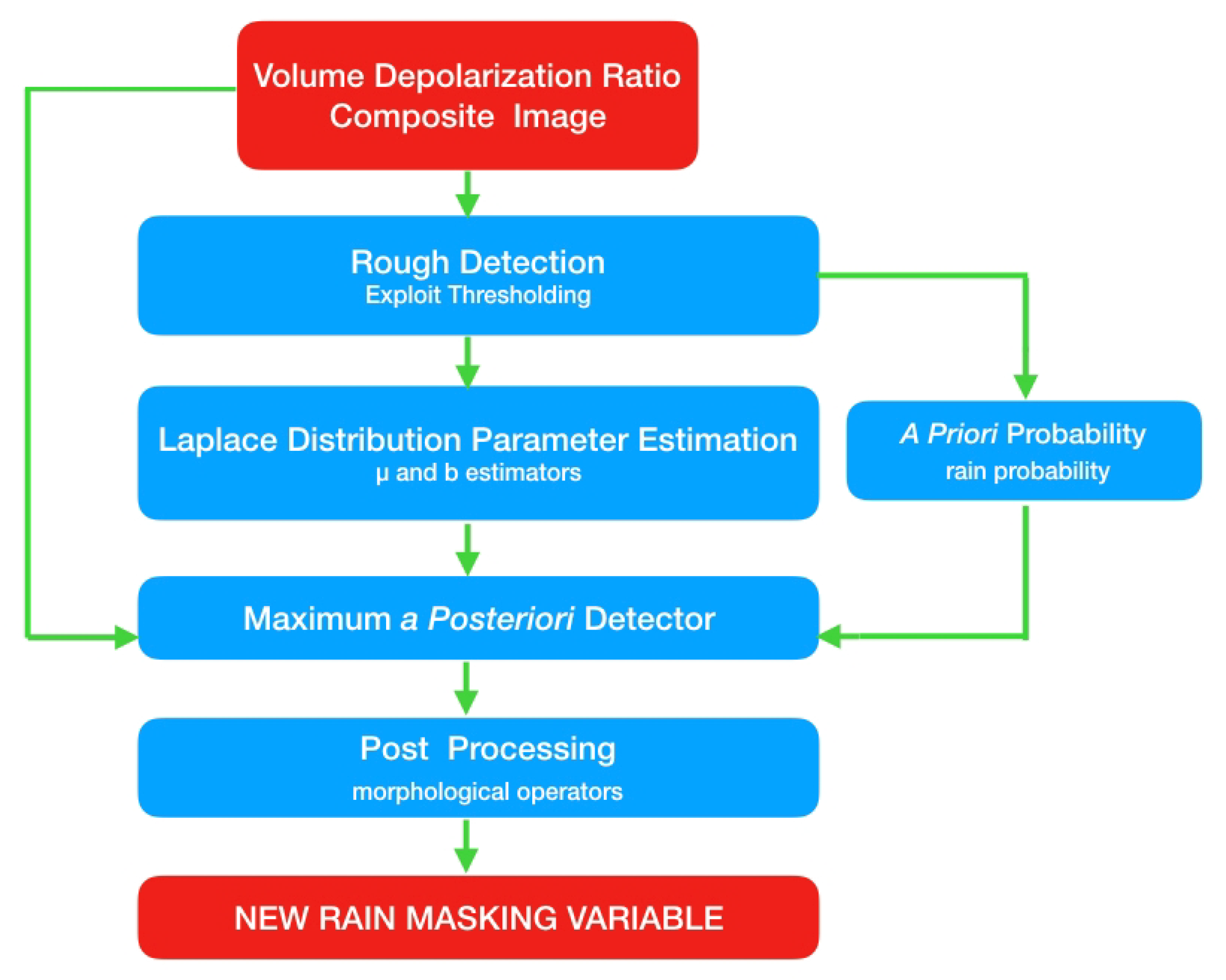
4.1. Processing Chain for Rain Detection

The proposed algorithm (flowchart shown in Figure 3) is based on image processing techniques.
The algorithm processes VDR composite images from the MPLNET L15 NRB product. Then, the VDR composite plot is paired with the cloud masking variable found in L15 CLD product, as precipitation detection is uniquely carried out under the cloud base, given by the cloud mask [13] (natural rain does not exist under clear sky conditions). Thus, the proposed rain detection algorithm will analyze only the VDR bins under the clouds. Afterwards, these bins are preliminarily labeled as “rain” if, and only if, they are above a certain threshold value (0.07, see Section 4.2.1). Non-rainy bins are those either not topped by a cloud or with a VDR value below the threshold (0 < VDR < 0.07). This preliminary rain mask is used to estimate the parameters of the Laplace distributions under the hypotheses r a i n and n o n r a i n and the rain a priori probability in order to use a maximum a posteriori (MAP) detector for estimating an accurate rain mask, see Section 4.2. Finally, a post-processing phase based on morphological operators is applied to reduce the image noise due to the signal extinction above the clouds and to remove any non-rectangular shaped detection, thus producing the final rain mask.
The algorithm is currently set-up to detect rain events for cloud bases at least 400 m above the surface and for rainfall episodes that last a minimum of 7 min. As a final step, all the detected rainfall events without any physical meaning are filtered out (i.e., precipitation not originating from the cloud base).

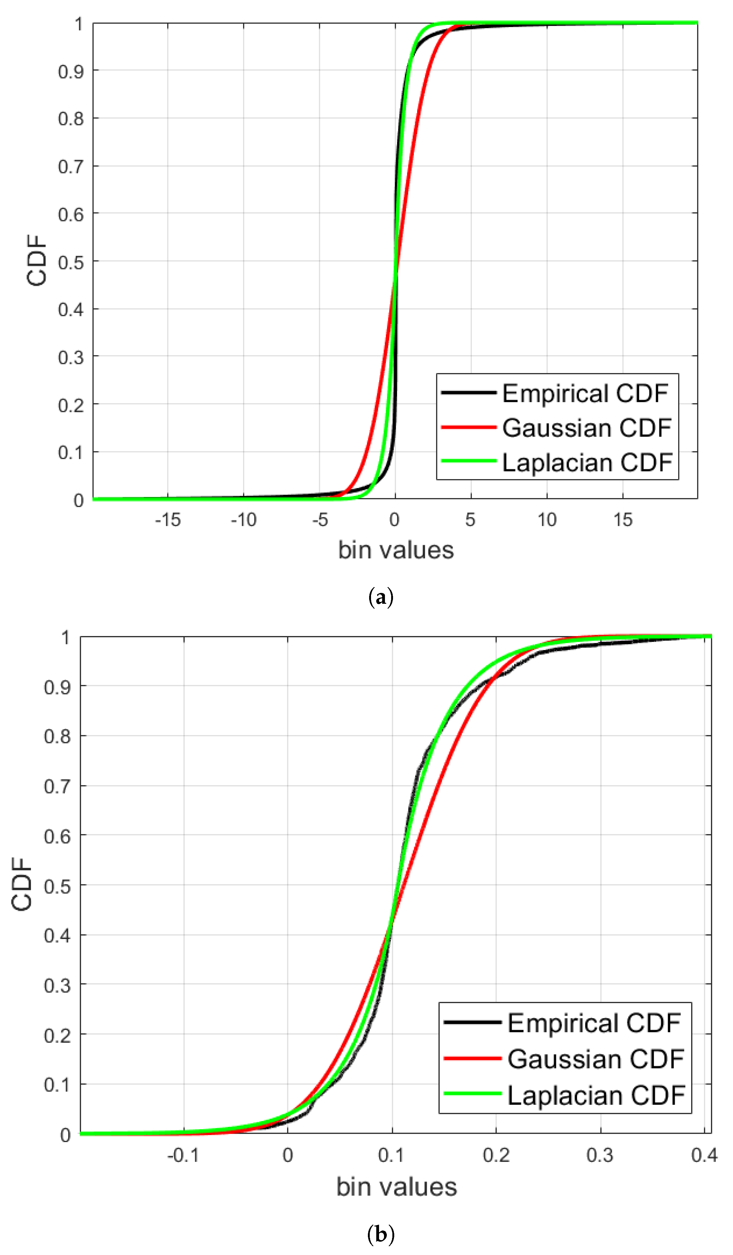
4.2. Maximum a Posterior Detector

To detect rainfall events, we use the previously described volume depolarization ratio composite image, which can be represented in a vectorial form as VDR = V D R 1 , , V D R i , , V D R n with V D R i R + , where n is the total number of bins. We also denote c = c 1 , , c i , , c n , as the vector of the labels in the set C = { n o n r a i n , r a i n } , where r a i n means that a generic V D R i is classified as “rain”, otherwise it belongs to the class “non-rain”. The detection problem is formalized into the Bayesian framework. Hence, the minimum Bayesian risk is achieved by the maximum a posterior probability (MAP) rule [30], i.e., we have
c ^ = arg max c p ( c | VDR ) = arg max c p ( VDR | c ) · p ( c ) ,
where p ( VDR | c ) is the likelihood and p ( c ) represents thea priori probability. The likelihood p ( VDR | c ) in Equation (1) can be simplified by the additional assumption of conditional independence among data. This yields its factorized form as follows
c ^ = arg max c 1 , , c n n i = 1 p ( V D R i | c i ) · p ( c i ) .
Thus, given c ^ = c ^ 1 , , c ^ i , , c ^ n , the problem of its maximization can be simply solved by maximizing each term, i.e., for each pixel i 1 , , n , we have:
c ^ i = arg max c i p ( V D R i | c i ) · p ( c i ) .
This leads to a binary hypothesis test that can be written as
Λ ( V D R i ) = p ( V D R i | c i = r a i n ) p ( V D R i | c i = n o n r a i n ) n o n r a i n r a i n p ( c i = n o n r a i n ) p ( c i = r a i n ) ,
where the likelihood ratio Λ ( V D R i ) is compared with the threshold p ( c i = n o n r a i n ) p ( c i = r a i n ) . If Λ ( V D R i ) > p ( c i = n o n r a i n ) p ( c i = r a i n ) , V D R i is classified as r a i n , otherwise V D R i is associated to the class n o n r a i n .
Under the assumption of Laplace distributed data for both the hypotheses (which have been experimentally validated, see Figure 4), the solution for each V D R i is
| V D R i μ n r | b n r | V D R i μ r | b r n o n r a i n r a i n γ ,
where
γ = log b n r · p ( c i = n o n r a i n ) b r · p ( c i = r a i n ) ,
log is the natural logarithm, μ r and b r are the location and scale parameters, respectively, which characterize the Laplace distribution under the r a i n hypothesis and μ n r and b n r are the related parameters for the n o n r a i n hypothesis.

4.2.1. Parameter Estimation

In order to estimate all the parameters in Equation (5), we exploit the lidar image under analysis and we find a first rough detection map, i.e., roughly identifying the rain bins. Thus, we apply a thresholding of the image’s bins to solve the rain detection problem. The used threshold has been experimentally set to 0.07 . After this preliminary step, we use the data labeled either as rain or as non-rain to estimate the parameters for both classes. Thus, given that n r independent and identically distributed samples belonging to a class r a i n , obtained selecting in VDR the r a i n bins, i.e., the ones detected as r a i n by the above-mentioned thresholding approach, we have that VDR r = [ V D R 1 r , , V D R i r , , V D R N r ] . In order to estimate the values of the a priori probability for both the classes, we count all these bins, which belong to the class r a i n in the rough detection map. Hence, if c o u n t ( · ) is the counter operator, p ( c i = r a i n ) = c o u n t ( VDR r ) n . p ( c i = n o n r a i n ) is simply equal to 1 p ( c i = r a i n ) .
The other parameters to be estimated are the ones related to the Laplace distribution. Focusing on the problem of the parameter estimations for the Laplace distribution under the class r a i n (all the considerations are equivalent even in the case of the estimations of the same parameters under the hypothesis of n o n r a i n ), the maximum likelihood estimators (MLEs) for μ r and b r are:
  • The MLE, μ ^ r , of μ r is μ ^ r = m e d ( VDR r ) , where m e d ( · ) is the sample median operator.
  • The MLE, b ^ r , of b r is the mean absolute deviation from the median, i.e.,
    b ^ r = 1 n r i = 1 n r V D R i r μ ^ r .

4.3. Post-Processing Based on Morphological Operators

In this section we highlight and describe the post-processing step to raise the MAP detector performance presented in Section 4.2. Morphological operators basis are first described referring to their application to a generic image, I , see Section 4.3.1. Their use for the problem at hand is instead described in Section 4.3.2.

4.3.1. Basics of Morphological Operators

An image I : E Z 2 V Z is analyzed by the morphological operators through the so-called structuring element (SE) B [31], which can be defined through its spatial support N B ( x ) , i.e., the neighborhood with respect to the position x E in which B is centered, and by its values. It is possible to characterize flat SEs by unitary values and the only free parameters for defining B in this case are the origin and N B .
Erosion ε B I and Dilation δ B I are the two basic operators defined for each point x I , as:
ε B I x = y N B x I y ; δ B I x = y N B x I y ,
where S and S are the infimum and supremum values within the set S, respectively.
The erosion (respectively, dilation) application has a filtering effect that suppresses bright (respectively, dark) regions smaller than B and the enlargement of dark (respectively, bright) ones. For bright and dark regions we mean that the local contrast in a certain region has intensity values respectively greater or lower with respect to the surrounding ones. Erosion and dilation operators can be recast into minimum and maximum operators on B, respectively, if I is a binary image. We also introduce, for convenience, the opening and closing that correspond to the two possible sequential compositions of erosion and dilation:
γ B I = δ B ˘ ε B I , ϕ B I = ε B ˘ δ B I ,
with B ˘ denoting the SE obtained by reflecting B with respect to its origin. A closing removes dark regions smaller than B while an opening suppresses bright ones. For further details about morphological operators, the interesting readers can refer to the related literature [31].

4.3.2. Use of Morphological Operators for Rain Detection Post-Processing

Two kinds of post-processing based on morphological operators are applied to the rain detection map coming from the MAP detector described in Section 4.2. In particular, given the detection map ( r a i n / n o n r a i n ) in matrix form, i.e., C ^ , we first apply a low-pass morphological filter to remove salt and pepper noise into C ^ to achieve a new low-pass version image denoted as C ^ L P . The low-pass morphological filter can be formulated by sequentially applying a closing operator and an opening operator with the same structuring element B 1 , i.e.,
C ^ L P = ϕ B 1 γ B 1 C ^ ,
where B 1 is a disk structuring element with a radius experimentally set to 4.
Last, but not least, the post-processing operation is based on an opening operator with a rectangular structuring element B 2 , i.e.,
C ^ P P = γ B 2 C ^ L P ,
where C ^ P P is the final map after the morphological post-processing. This last processing is performed to delete detected objects that do not follow a rectangular shape with some constraints about the minimal size. In particular, the minimal sizes of the sides of the rectangle are tunable parameters that are selected to 7 (i.e., 7 min) that is the minimal temporal resolution to consider that is raining (i.e., we are not able to detect rains that last less than 7 min), and about 2.67 for the other side. This value takes into account of the minimal vertical dimension of the rains and coming from the fact that the data has a spatial resolution of 75 m, thus, we have a minimum vertical dimension of the rains equal to 200 m. Therefore, only these kinds of detected objects have the right spatial features to be considered rain. These parameters have been tuned for this specific problem and type of data. Obviously, considering lidar data with different features will lead to a new tuning of parameters in order to achieve high performance.

5. Results

5.1. Intercomparison with Ground-Based Disdrometer Measurements

The algorithm results are compared against rain intensity measurements obtained from a co-located disdrometer, an in-situ measurement device designed to measure the drop size distribution (DSD) [10], represented as the number of drops per unit of volume and per unit of raindrop diameter. Disdrometers can be based on different measurement principles (high-speed cameras, Doppler effect, laser-optical, impact, etc.). The second generation Parsivel (Parsivel 2 ) laser-optical disdrometer manufactured by OTT [32] is used in this work. Parsivel systems were originally developed by PM Tech Inc., Germany. The instrument has a laser diode (emitting wavelength of 780 nm) generating a horizontal flat beam with a measurement area of 54 cm 2 .
The disdrometer principle of operation is based on laser technology. When a hydro-meteor passes through a volume uniformly illuminated by a laser beam, it produces a temporal attenuation proportional to its size with a duration depending on its fall speed. A relationship between the laser beam occlusion by the falling particle is applied to estimate the particle size. Parsivel instruments can measure particle diameters up to about 25 mm classifying them in 32 size classes of different widths. The instrument also estimates the hydro-meteor fall velocity by measuring the time necessary for the particle to pass through the laser beam, and thus stores particles in 32 × 32 matrices. The disdrometers high temporal resolution (60 s for this work) permits study in great detail of physical precipitation variability.

5.2. Rain Detection Algorithm Working under Simpler and Complex Meteorological Conditions

In this section we show how the rain masking algorithm works in different meteorological conditions, i.e., for light and stronger precipitation intensities. The comparison results are carried out at the NASA Goddard Space Flight Center (GSFC) MPLNET permanent observational site (Lat: 38.9 N, Lon: 76.3 W, Alt: 50 m a.s.l.), where measurement data from a co-located Parsivel 2 disdrometer are also available. The rain masking algorithm can also detect the so-called virga streaks (Figure 5), a kind of precipitation that, due to the strong evaporation, will never reach the ground [5]. As can be easily understood, virga episodes cannot be detected by the disdrometers.

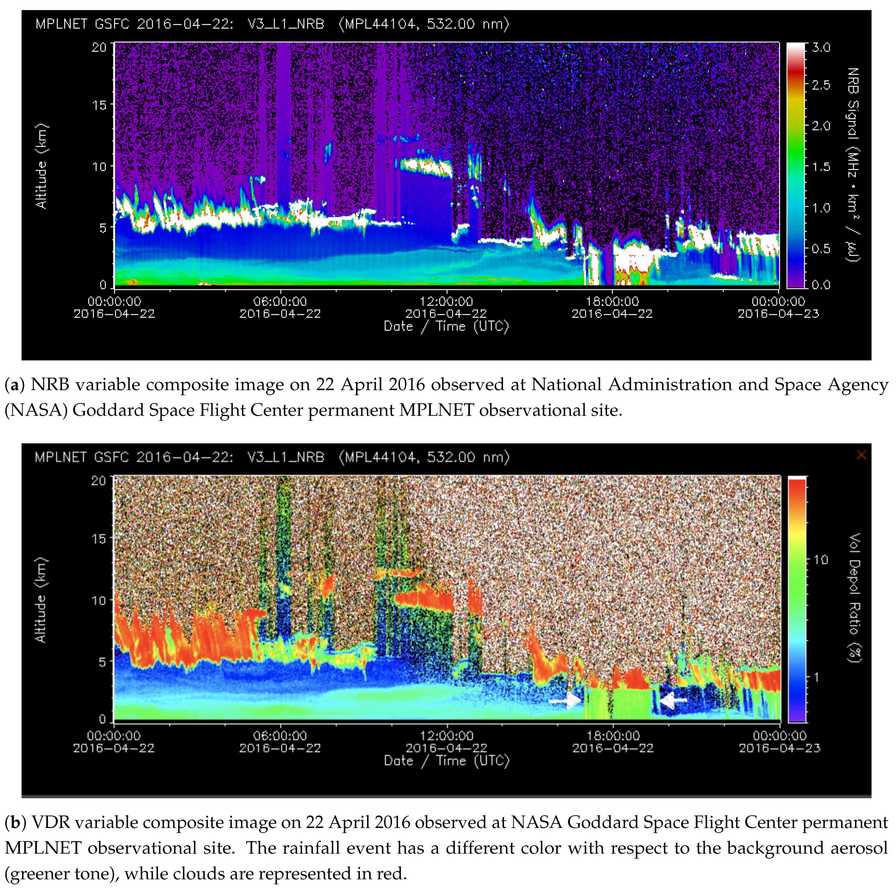
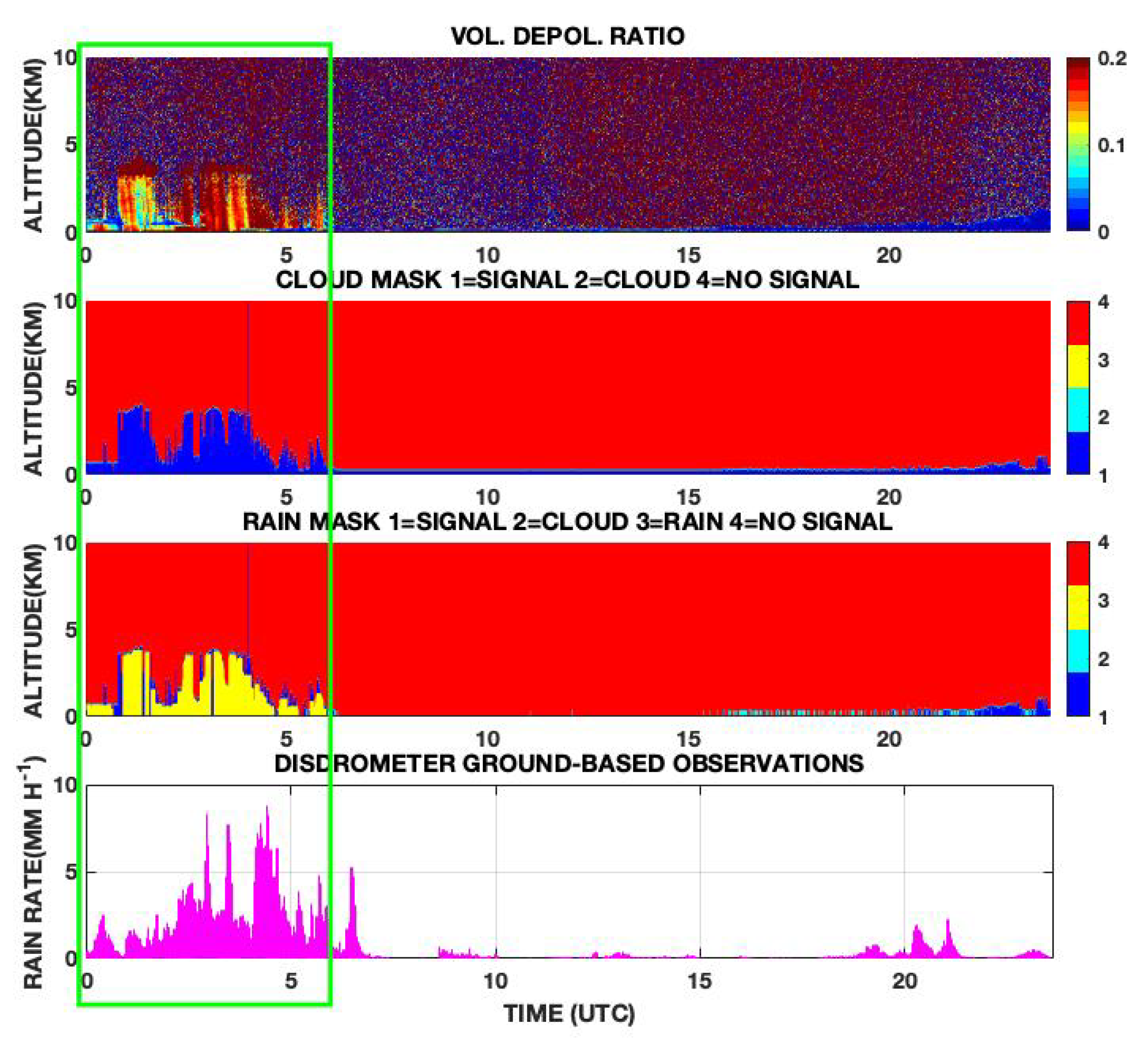
5.2.1. A Simple Case: 22 April 2016

As described in Section 4.2, the rain detection algorithm first step consists in pairing VDR composite images with the L15 cloud masking variable. Then, a first guess of rain probability is produced only for the VDR signal above a certain threshold and below a cloud base, i.e., on deep blue regions topped by cyan cloud regions of upper middle plots of Figure 5. The detection in this case does not show any critical aspects. The cloud base is never below 400 m and the precipitation intensity is very low, i.e., 0.25 mm h−1 on daily average. Those intensities cannot completely attenuate the lidar signal. Two virga streaks are detected by the algorithm in the second half of the day. The retrieved disdrometer rain rate (Figure 5; bottom), shows very low values, with a maximum of 0.76 mm h−1 at 1701 UTC. Globally, there is a partial agreement between the disdrometer and the rain masking algorithm: After 1815 UTC rain intensity drops so much that the disdrometer is unable to detect the precipitation, while after 2200 UTC, the rain masking algorithm fails to detect the rainfall up to the ground. Precipitation events from lidar data are then necessary to fill a gap in detecting very low precipitation intensity events (<0.05 mm h−1) that are crucial to study the aerosol effects and interactions on clouds and rainfall [33].

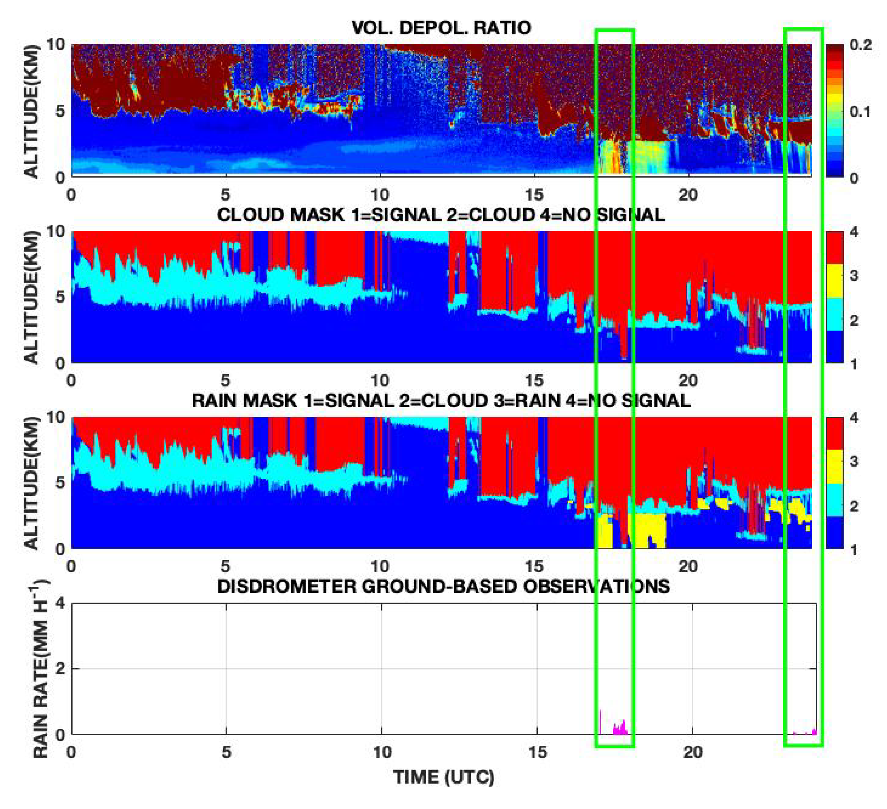
5.2.2. Intermittent Rain: 12 April 2016

The meteorological situation is more complex with respect to the previous case. In the upper composite plot (the volume depolarization ratio) of Figure 6 we can notice the transit of a front over the observational site with a progressive descent of the cloud base from 0000 UTC to about 0530 UTC. The precipitation is intermittent and at least four events are detected by the algorithm. The rainfall intensity is still low, as shown by in-situ disdrometer observations (Figure 6): the average intensity during the day is 0.9 mm h−1, with a peak of 12 mm h−1 around 1300 UTC that lasts only less than 5 min. The precipitation event at 0600 UTC in the rain mask is not detected by the disdrometer as the precipitation intensity is below its sensitivity (0.05 mm h−1).

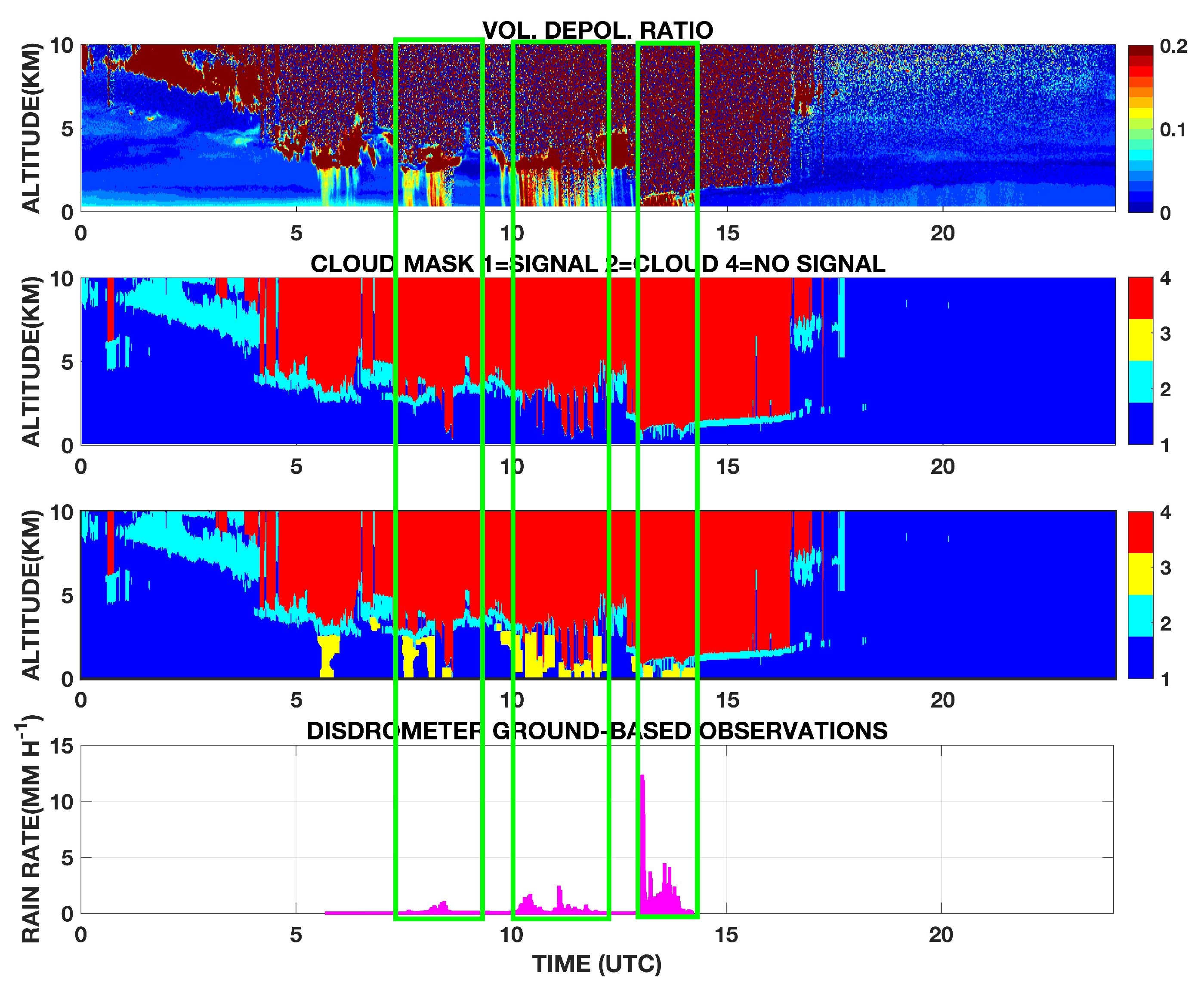
5.2.3. Lighter Rain Followed by Stronger Rain: Case of 10 November 2015

During this day, the precipitation is more intense with respect to the the previous two cases, with an average intensity recorded, from 0000 UTC to 0700 UTC, of about 3.7 mm h−1. Higher peaks of rain rates of about 8.8 mm h−1, lasting more than 30 min, completely soak the telescope and receiver optics making it impossible to perform any further detection by the algorithm, as shown in Figure 7. The disdrometer shows that precipitation, even with a lower intensity, lasted almost the whole day. But after 0600 UTC the cloud base drops below 400 m making the detection by the algorithm impossible. This rainfall event highlights the limits of the lidar technology in detecting precipitation under very low signal to noise ratio [34]. From Figure 7 it is possible to fix a detection limit threshold depending on rain intensity and duration, i.e., rain rate > 8 mm h−1 lasting > 30 min.

5.3. Overall Intercomparison

The rain detection algorithm has been intercompared with ground-based disdrometer observations over 7 days between November 2015 and April 2016. The intercomparison, as stated before, was carried out at NASA Goddard Space Flight Center. Table 1 summarizes all the precipitation events, together with their lengths used, for the intercomparison.
As shown in Table 1, the algorithm performances are tested vs. the disdrometer observations. The detected precipitation events by the rain masking algorithm and the ground based disdrometers have different sensitivities, i.e., the lidar instrument can detect rainfall episodes not reaching the ground while the disdrometer can not detect intensities lower than 0.05 mm h−1. On the contrary, higher intensity precipitation (at least 30 min with a rain rate > 8 mm h−1, see Figure 7) can not be detected by the rain algorithm as the lidar signal is completely extinguished. It is important to stress that the rain masking algorithm has a 100% (14/14) success rate in detecting disdrometer observed precipitation. A detection is considered successful if the disdrometer observation and the algorithm detection share at least one minute in common, independently of the total precipitation duration, which can be different for the reasons previously explained.
Analysis from Table 1, shows that the algorithm is more sensitive at detecting lower intensity precipitation by 22% (4/18). If we examine the bias with respect to precipitation start and stop (see Table 1, fifth column), we found that the detection algorithm precedes the disdrometer observations by about 9 min, while the opposite is true in detection of the precipitation end, where the disdrometer lasts 5.5 min longer. This can be partially attributed to the water soaking the lidar telescope window with a consequent fully attenuated signal.
Overall, the disdrometer measured 1084 min of precipitation vs. 1095 min of detected precipitation by the algorithm. We also calculated the root mean square error (RMSE) with respect to the precipitation global duration as defined in [4], and we found that the average absolute difference in precipitation total duration detected by the algorithm and measured by the disdrometer is of about 10.23 min. Considering the different characteristics of the ground-based instrument and the detection algorithm, the agreement is within reason.

6. Discussion and Conclusions

Automated networks of instruments started to develop in the last two decades aiming to continuously monitor crucial atmospheric physical, thermodynamic, geometrical, and optical variables. Among them, the NASA MicroPulse Lidar NETwork (MPLNET), active since 1999, has globally deployed more than 21 worldwide observational sites in the tropics, mid-latitudes, and polar regions in both hemispheres to automatically retrieve 24/24 the geometrical and optical properties of aerosol and cloud atmospheric profiles under any meteorological conditions. Despite that lidar has proven to be very effective in detecting especially light precipitation and drizzle, lidar data containing precipitation episodes are currently unjustifiably disregarded. As a proof of concept, in this study we developed a rain masking algorithm, based on the volume depolarization ratio variable, which is proven to be effective in detecting light rain, drizzle, and virga episodes. Once rigorously validated and operationally implemented into the NASA MPLNET lidar network, the rain masking algorithm will consistently help in understanding how light precipitation contributes to cloud formation and will fill a gap left by TRMM and GPM missions in detecting low intensity rainfall episodes. This is crucial to improving global climate model forecasts and for aerosol–clouds and in turn, precipitation interactions. Finally, as future development, the algorithm will be also tested on simpler elastic lidar instruments without the depolarization channel, i.e., the ceilometers, to assess the rain detection feasibility. In more detail, precipitation is a fundamental meteorological phenomenon that is the principal responsible for atmospheric aerosol removal. Analyzing a large database of lidar measurements will help in fully characterizing the aerosol cycle, from emission to deposition, and validate global model observations that show a strong negative correlation between Aerosol Optical Depth (AOD) and precipitation due to wet scavenging [35]. A synergy between both passive and active satellite NASA missions, i.e., the Moderate Resolution Imager Spectrometer (MODIS; [36] and the Cloud-Aerosol Lidar and Infrared Pathfinder Satellite Observation (CALIPSO; [37]), and the ground based lidar networks, such as the European Aerosol LIdar NETwork (EARLINET; [38]) part of the Aerosols, Clouds and Trace gases Research Infrastructure (ACTRIS http://www.actris.eu) and in North America as MPLNET, and more in general in the frame of Global Aerosol Watch (GAW) aerosol lidar observation network (GALION; [39]) will strongly contribute to quantitatively assess how the above cloud aerosol load influences clouds and then rainfalls. The synergy will then assess the “all-sky” aerosol contribution to clouds and precipitation.
The image-based technique methodology used in developing the proposed algorithm, will be tested in a future work over different instruments, i.e., ceilometers, where precipitation still looks like a higher-contrasted feature in the range corrected backscattered energy.

Author Contributions

Conceptualization, S.L., G.V., J.R.L., E.J.W.; methodology, S.L., G.V., J.R.L., E.J.W., M.S., and A.C.; software, G.V.; validation, S.L., G.V., J.R.L., E.J.W., M.S., A.C., and L.P.D.; formal analysis, S.L.; investigation, S.L., J.R.L., E.J.W., M.S. and A.C.; resources, E.J.W., G.P. and A.T.; data curation, A.T., L.P.D., E.J.W. and A.G.; writing–original draft preparation, S.L.; writing–review and editing, S.L., J.R.C., A.C., M.S., L.P.D., G.P. and A.G.; visualization, G.P.; supervision, G.P.; project administration, A.C., E.J.W., G.P.; funding acquisition, S.L. and E.J.W. All authors have read and agreed to the published version of the manuscript.

Funding

This research was funded by the Italian Research Council (CNR) Short Term Mobility Program. The NASA Micro-Pulse Lidar Network is supported by the NASA Earth Observing System (S. Platnick) and Radiation Sciences Program (H. Maring).

Conflicts of Interest

The authors declare no conflict of interest.

References

  1. Bosilovich, M.G.; Schubert, S.D.; Walker, G.K. Global Changes of the Water Cycle Intensity. J. Clim. 2005, 18, 1591–1608. [Google Scholar] [CrossRef] [Green Version]
  2. Koster, R.D.; Suarez, M.J.; Heiser, M. Variance and Predictability of Precipitation at Seasonal-to-Interannual Timescales. J. Hydrometeorol. 2000, 1, 26–46. [Google Scholar] [CrossRef]
  3. Lolli, S.; Di Girolamo, P. Principal component analysis approach to evaluate instrument performances in developing a cost-effective reliable instrument network for atmospheric measurements. J. Atmos. Ocean. Technol. 2015, 32, 1642–1649. [Google Scholar] [CrossRef]
  4. Lolli, S.; Delaval, A.; Loth, C.; Garnier, A.; Flamant, P. 0.355-micrometer direct detection wind lidar under testing during a field campaign in consideration of ESA’s ADM-Aeolus mission. Atmos. Meas. Tech. 2013, 6, 3349–3358. [Google Scholar] [CrossRef] [Green Version]
  5. Lolli, S.; D’Adderio, L.; Campbell, J.; Sicard, M.; Welton, E.; Binci, A.; Rea, A.; Tokay, A.; Comerón, A.; Baldasano, R.B.J.M.; et al. Vertically Resolved Precipitation Intensity Retrieved through a Synergy between the Ground-Based NASA MPLNET Lidar Network Measurements, Surface Disdrometer Datasets and an Analytical Model Solution. Remote Sens. 2018, 10, 1102. [Google Scholar] [CrossRef] [Green Version]
  6. Campbell, J.R.; Ge, C.; Wang, J.; Welton, E.J.; Bucholtz, A.; Hyer, E.J.; Reid, E.A.; Chew, B.N.; Liew, S.C.; Salinas, S.V.; et al. Applying advanced ground-based remote sensing in the Southeast Asian Maritime Continent to characterize regional proficiencies in smoke transport modeling. J. Appl. Meteorol. Climatol. 2016, 55, 3–22. [Google Scholar] [CrossRef]
  7. Westbrook, C.; Hogan, R.; O’Connor, E.; Illingworth, A. Estimating drizzle drop size and precipitation rate using two-colour lidar measurements. Atmos. Meas. Tech. 2010, 3, 671–681. [Google Scholar] [CrossRef] [Green Version]
  8. Lolli, S.; Welton, E.J.; Campbell, J.R. Evaluating light rain drop size estimates from multiwavelength micropulse lidar network profiling. J. Atmos. Ocean. Technol. 2013, 30, 2798–2807. [Google Scholar] [CrossRef] [Green Version]
  9. Lolli, S.; Di Girolamo, P.; Demoz, B.; Li, X.; Welton, E. Rain Evaporation Rate Estimates from Dual-Wavelength Lidar Measurements and Intercomparison against a Model Analytical Solution. J. Atmos. Ocean. Technol. 2017, 34, 829–839. [Google Scholar] [CrossRef]
  10. D’Adderio, L.; Porcù, F.; Tokay, A. Evolution of drop size distribution in natural rain. Atmos. Res. 2018, 200, 70–76. [Google Scholar] [CrossRef]
  11. Omar, A.H.; Winker, D.M.; Vaughan, M.A.; Hu, Y.; Trepte, C.R.; Ferrare, R.A.; Lee, K.P.; Hostetler, C.A.; Kittaka, C.; Rogers, R.R.; et al. The CALIPSO automated aerosol classification and lidar ratio selection algorithm. J. Atmos. Ocean. Technol. 2009, 26, 1994–2014. [Google Scholar] [CrossRef]
  12. Papagiannopoulos, N.; Mona, L.; Amodeo, A.; D’Amico, G.; Gumà Claramunt, P.; Pappalardo, G.; Alados-Arboledas, L.; Guerrero-Rascado, J.L.; Amiridis, V.; Kokkalis, P.; et al. An automatic observation-based aerosol typing method for EARLINET. Atmos. Chem. Phys. 2018, 18, 15879–15901. [Google Scholar] [CrossRef] [Green Version]
  13. Lewis, J.R.; Campbell, J.R.; Welton, E.J.; Stewart, S.A.; Haftings, P.C. Overview of MPLNET Version 3 Cloud Detection. J. Atmos. Ocean. Technol. 2016, 33, 2113–2134. [Google Scholar] [CrossRef]
  14. Flynn, C.J.; Mendoza, A.; Zheng, Y.; Mathur, S. Novel polarization-sensitive micropulse lidar measurement technique. Opt. Express 2007, 15, 2785–2790. [Google Scholar] [CrossRef]
  15. Hou, A.Y.; Kakar, R.K.; Neeck, S.; Azarbarzin, A.A.; Kummerow, C.D.; Kojima, M.; Oki, R.; Nakamura, K.; Iguchi, T. The Global Precipitation Measurement Mission. Bull. Am. Meteorol. Soc. 2014, 95, 701–722. [Google Scholar] [CrossRef]
  16. Kidd, C.; Joe, P. Importance, identification and measurement of light precipitation at mid-to high-latitudes. In Proceedings of the Joint EUMETSAT Meteorological Satellite Conference and 15th Satellite Meteorology and Oceanography Conference, Amsterdam, The Netherlands, 24–28 September 2007; pp. 24–28. [Google Scholar]
  17. Welton, E.J.; Campbell, J.R.; Spinhirne, J.D.; Stanley Scott, V., III. Global monitoring of clouds and aerosols using a network of micropulse lidar systems. SPIE Conf. Proc. 2001, 4153, 151–158. [Google Scholar]
  18. Spinhirne, J.D.; Rall, J.A.; Scott, V.S. Compact Eye Safe Lidar Systems. Rev. Laser Eng. 1995, 23, 112–118. [Google Scholar] [CrossRef] [Green Version]
  19. Ciofini, M.; Lapucci, A.; Lolli, S. Diffractive optical components for high power laser beam sampling. J. Opt. Pure Appl. Opt. 2003, 5, 186. [Google Scholar] [CrossRef]
  20. Wielicki, B.A.; Cess, R.D.; King, M.D.; Randall, D.A.; Harrison, E.F. Mission to planet Earth: Role of clouds and radiation in climate. Bull. Am. Meteorol. Soc. 1995, 76, 2125–2154. [Google Scholar] [CrossRef]
  21. Pani, S.K.; Wang, S.H.; Lin, N.H.; Tsay, S.C.; Lolli, S.; Chuang, M.T.; Lee, C.T.; Chantara, S.; Yu, J.Y. Assessment of aerosol optical property and radiative effect for the layer decoupling cases over the northern South China Sea during the 7-SEAS/Dongsha Experiment. J. Geophys. Res. Atmos. 2016, 121, 4894–4906. [Google Scholar] [CrossRef]
  22. Tosca, M.G.; Campbell, J.; Garay, M.; Lolli, S.; Seidel, F.C.; Marquis, J.; Kalashnikova, O. Attributing accelerated summertime warming in the southeast united states to recent reductions in aerosol burden: Indications from vertically-resolved observations. Remote Sens. 2017, 9, 674. [Google Scholar] [CrossRef] [Green Version]
  23. Lolli, S.; Madonna, F.; Rosoldi, M.; Campbell, J.R.; Welton, E.J.; Lewis, J.R.; Gu, Y.; Pappalardo, G. Impact of varying lidar measurement and data processing techniques in evaluating cirrus cloud and aerosol direct radiative effects. Atmos. Meas. Tech. 2018, 11, 1639. [Google Scholar] [CrossRef] [Green Version]
  24. Campbell, J.R.; Lolli, S.; Lewis, J.R.; Gu, Y.; Welton, E.J. Daytime cirrus cloud top-of-the-atmosphere radiative forcing properties at a midlatitude site and their global consequences. J. Appl. Meteorol. Climatol. 2016, 55, 1667–1679. [Google Scholar] [CrossRef]
  25. Lolli, S.; Campbell, J.R.; Lewis, J.R.; Gu, Y.; Marquis, J.W.; Chew, B.N.; Liew, S.C.; Salinas, S.V.; Welton, E.J. Daytime Top-of-the-Atmosphere Cirrus Cloud Radiative Forcing Properties at Singapore. J. Appl. Meteorol. Climatol. 2017, 56, 1249–1257. [Google Scholar] [CrossRef] [Green Version]
  26. Holben, B.; Eck, T.; Slutsker, I.; Tanré, D.; Buis, J.; Setzer, A.; Vermote, E.; Reagan, J.; Kaufman, Y.; Nakajima, T.; et al. AERONET—A Federated Instrument Network and Data Archive for Aerosol Characterization. Remote Sens. Environ. 1998, 66, 1–16. [Google Scholar] [CrossRef]
  27. Welton, E.J.; Campbell, J.R. Micropulse Lidar Signals: Uncertainty Analysis. J. Atmos. Ocean. Technol. 2002, 19, 2089–2094. [Google Scholar] [CrossRef]
  28. Bissonnette, L.R.; Roy, G.; Fabry, F. Range–Height Scans of Lidar Depolarization for Characterizing Properties and Phase of Clouds and Precipitation. J. Atmos. Ocean. Technol. 2001, 18, 1429–1446. [Google Scholar] [CrossRef]
  29. Campbell, J.R.; Hlavka, D.L.; Welton, E.J.; Flynn, C.J.; Turner, D.D.; Spinhirne, J.D.; Scott, V.S.; Hwang, I.H. Full-Time, Eye-Safe Cloud and Aerosol Lidar Observation at Atmospheric Radiation Measurement Program Sites: Instruments and Data Processing. J. Atmos. Ocean. Technol. 2002, 19, 431–442. [Google Scholar] [CrossRef]
  30. Kay, S. Fundamentals of Statistical Signal Processing: Detection Theory; Fundamentals of Statistical Signal Processing; PTR Prentice-Hall: Upper Saddle River, NJ, USA, 1993. [Google Scholar]
  31. Soille, P. Morphological Image Analysis: Principles and Applications; Springer-Verlag: Berlin/Heidelberg, Germany, 2003. [Google Scholar]
  32. Löffler-Mang, M.; Joss, J. An Optical Disdrometer for Measuring Size and Velocity of Hydrometeors. J. Atmos. Ocean. Technol. 2000, 17, 130–139. [Google Scholar] [CrossRef]
  33. Yum, S.S.; Cha, J.W. Suppression of very low intensity precipitation in Korea. Atmos. Res. 2010, 98, 118–124. [Google Scholar] [CrossRef]
  34. Alparone, L.; Selva, M.; Aiazzi, B.; Baronti, S.; Butera, F.; Chiarantini, L. Signal-dependent noise modelling and estimation of new-generation imaging spectrometers. In Proceedings of the WHISPERS 2009, Grenoble, France, 26–28 August 2009. [Google Scholar]
  35. Gryspeerdt, E.; Stier, P.; White, B.A.; Kipling, Z. Wet scavenging limits the detection of aerosol effects on precipitation. Atmos. Chem. Phys. 2015, 15, 7557–7570. [Google Scholar] [CrossRef] [Green Version]
  36. Remer, L.A.; Kaufman, Y.; Tanré, D.; Mattoo, S.; Chu, D.; Martins, J.V.; Li, R.R.; Ichoku, C.; Levy, R.; Kleidman, R.; et al. The MODIS aerosol algorithm, products, and validation. J. Atmos. Sci. 2005, 62, 947–973. [Google Scholar] [CrossRef] [Green Version]
  37. Hunt, W.H.; Winker, D.M.; Vaughan, M.A.; Powell, K.A.; Lucker, P.L.; Weimer, C. CALIPSO lidar description and performance assessment. J. Atmos. Ocean. Technol. 2009, 26, 1214–1228. [Google Scholar] [CrossRef]
  38. Pappalardo, G.; Amodeo, A.; Apituley, A.; Comeron, A.; Freudenthaler, V.; Linné, H.; Ansmann, A.; Bösenberg, J.; D’Amico, G.; Mattis, I.; et al. EARLINET. Atmos. Meas. Tech. 2014, 7, 2389–2409. [Google Scholar] [CrossRef] [Green Version]
  39. Bösenberg, J.; Hoff, R. Plan for the Implementation of the GAW Aerosol Lidar Observation Network GALION:(Hamburg, Germany, 27–29 March 2007); GAW Report 178; WMO: Geneva, Switzerland, 2007. [Google Scholar]
Figure 1. 27 March 2017 Micropulse lidar network (MPLNET) Version 3 Volume Depolarization Ratio (VDR) variable (L15 MPLNET Normalized Relative Backscattering (NRB) product). Red arrows highlight the starting point of the precipitation events.
Remotesensing 12 00071 g001
Figure 2. Precipitation event detected on 22 April 2016. With respect to (a) NRB, the precipitation on (b) VDR has more defined and sharp contours. The precipitation under the cloud (in red) has a different green tone. For this reason, the detection is easier on (b).
Remotesensing 12 00071 g002
Figure 3. Flowchart of V3 MPLNET rain detection algorithm. Red boxes indicate data input/output, while blue boxes represent the processing steps. A detailed description of all the steps can be found in the text.
Remotesensing 12 00071 g003
Figure 4. Cumulative distribution functions (CDFs) for (a) n o n r a i n VDR data and (b) r a i n VDR data. The empirical CDFs are the estimated CDFs from the data, i.e., considering n o n r a i n data in (a) and r a i n data in (b).
Remotesensing 12 00071 g004
Figure 5. Rain mask variable from rain detection algorithm on 22 April 2016 from MPLNET observation at NASA GSFC (Lat: 38.99 N, Lon: 76.38 W, Alt: 50 m a.s.l.). The different steps to obtain the rain mask are shown in the flowchart in Figure 3: Upper: Volume depolarization ratio variable obtained from MPLNET NRB L15 signal product. Middle 1: Cloud mask variable from MPLNET L15 CLD product. The algorithm retrieves precipitation only on blue regions topped by clouds (cyan bins). Middle 2: New rain mask product (rain plotted in yellow). Lower: Co-located precipitation intensity measured by disdrometer. The green rectangular shapes help in visualizing the detected rain events.
Remotesensing 12 00071 g005
Figure 6. Similar to Figure 5, but for 12 April 2016. This case presents different short precipitation originating from the transit of a front.
Remotesensing 12 00071 g006
Figure 7. Same as Figure 6, but for 10 November 2015. After 0600 UTC, the signal is completely extinguished making any detection impossible.
Remotesensing 12 00071 g007
Table 1. Precipitation events observed by Parsivel 2 at NASA GSFC used to validate the rain detection algorithm. The three values reported in the fifth column are the differences in minutes between disdrometer and algorithm in detecting precipitation. The first value represents the difference in minutes with respect to the precipitation start, the second one the same but for the precipitation end, while the third represents the difference in minutes on overall precipitation duration.
Event nr.DayDisdrometerLidarDiff. (min)
109 November 20152034–20512026–2042 8 / 9 / 1
209 November 20152140-00002214–0000 + 34 / 0 / 34
310 November 20150000–06000000–0600 0 / 0 / 0
430 November 20151300–13511328–1347 28 / 4 / 32
530 November 20151431–14451431–1459 0 / + 14 / + 14
617 December 20151216–12591212–1432 4 / + 93 / + 97
712 April 201605470534–0605 13 / 18 / + 30
812 April 20160735–08430730–0743
812 April 20160735–08430803–0815 5 / + 3 / 19
812 April 20160735–08430822–0846
912 April 20161005–12231000–1214 5 / 9 / 4
1012 April 20161255–14131246–1415 9 / + 2 / + 11
1122 April 20161727–17531659–1731 28 / 22 / + 6
1222 April 2016———1809–1842———
1322 April 2016———1858–1915———
1422 April 20162315–00002230–0000 45 / 0 / + 45
1523 April 20160000–01100000–0101 0 / 9 / 9
1623 April 2016———1423–1458———
1723 April 20161247–13201300–1320 13 / 0 / 13
1823 April 2016———1728–1937———

