Retrieval of Water Quality Parameters from Hyperspectral Images Using Hybrid Bayesian Probabilistic Neural Network

Abstract

The protection of water resources is of paramount importance to human beings’ practical lives. Monitoring and improving water quality nowadays has become an important topic. In this study, a novel Bayesian probabilistic neural network (BPNN) improved from ordinary Bayesian probability methods has been developed to quantitatively predict water quality parameters including phosphorus, nitrogen, chemical oxygen demand (COD), biochemical oxygen demand (BOD), and chlorophyll a. The proposed method, based on conventional Bayesian probability methods, involves feature engineering and deep neural networks. Additionally, it extracts significant information for each endmember from combinations of spectra by feature extraction, with spectral unmixing based on mathematical and statistical analysis, and calculates each of the water quality parameters. The experimental results show the great performance of the proposed model with all coefficient of determination $R^2$ over 0.9 greater than the values (0.6–0.8) from conventional methods, which are greater than ordinary Bayesian probability analysis. The mean percent of absolute error (MPAE) is taken into account as an important statistical criterion to evaluate model performance, and our results show that MPAE ranges from 4% (nitrogen) to 10% (COD). The root mean squared errors (RMSEs) of phosphorus, nitrogen, COD, BOD, and chlorophyll-a (Chla) are 0.03 mg/L, 0.28 mg/L, 3.28 mg/L, 0.49 mg/L, and 0.75 μg/L, respectively. In comparison with other deep learning methods, this study takes a relatively small amount of data as training data to train the proposed model and the proposed model is then tested on the same amount of testing data, achieving a greater performance. Thus, the proposed method is time-saving and more effective. This study proposes a more compatible and effective method to assist with decomposing combinations of hyperspectral signatures in order to calculate the content level of each water quality parameter. Moreover, the proposed method is practically applied to hyperspectral image data on board an unmanned aerial vehicle in order to monitor the water quality on a large scale and trace the location of pollution sources in the Maozhou River, Guangdong Province of China, obtaining well-explained and significant results.

1. Introduction

Monitoring the change in water quality through remote sensing techniques has recently become a topic of major interest. Thus, maintaining water of good quality is highly important and necessary. An efficient and labor-saving method for quantitatively computing the content level of five water quality parameters including phosphorus, nitrogen, biochemical oxygen demand (BOD), chemical oxygen demand (COD), and chlorophyll-a (Chla) has been developed due to the practical needs of human beings’ lives. Phosphorus and nitrogen are associated with eutrophication [1,2] and severe eutrophication can cause the considerable accumulation of Chla [3]. High levels of Chla may cause the death of aquatic creatures such as fish and shrimp and the amount of aquatic life, including aquatic animals and plants, is highly associated with levels of BOD and COD [4]. In the past few years, multispectral remote sensing as an orthodox method was an important method to categorize the level of water quality [5].

Nowadays, although methods of multispectral remote sensing analysis for the quantitative estimation of water quality parameters have obtained relatively accurate results, they are time-consuming and expensive [6]. Another hyperspectral remote sensing method has quickly developed due to practical needs not only for categorizing the level of water quality, but also for the cost-efficient and time-saving quantitative analysis of water quality parameters. A wide variety of methods concerning remote sensing to categorize the level of water quality or to assess the content level of water quality parameters mainly include empirical methods [7,8,9], semi-analytical methods [10,11], and deep learning methods [12,13,14] to quantify water quality parameters and classify water quality level through hyperspectral data [15]. For example, Gholizadeh et al. [7] proposed an empirical method of regression featuring band ratios and band combinations to assess the content level of water quality parameters including phosphorus, COD, BOD, and Chla, which selected bands based on the spectral features of target objects. Li et al. [8] proposed another empirical method to estimate Chla content with a relative percent difference (RPD) less than 30.45% at a high solar zenith angle. Another empirical method [9] sought to find band combinations that result in the strongest correlation by regression-given features against the content level of the target object, which gave a relatively high $R^2$ over 0.7 for some water quality parameters, including Chla, suspended solids, and colored dissolved organic matter. Furthermore, Campbell et al. [11] came up with a semi-analytical matrix inversion method (MIM) which aimed at quantitatively predicting Chla content with Medium Resolution Imaging Spectrometer (MERIS) images of an in-water light field with a mean difference of 1.0 μg/L. Chebud et al. [12] proposed an Artificial Neural Network (ANN) method to estimate the water quality parameters of phosphorus, turbidity, and Chla quantitatively with over 0.95 $R^2$ value, and the root mean squared error (RMSE) 0.17 mg/m³, 0.5 nephelometric turbidity unit (NTU), and 0.03 mg/L, respectively. Moreover, Pyo et al. [14] proposed a convolutional neural network (CNN) with the purpose of regression in terms of the water quality parameter Chla, which gave 0.73 as the $R^2$ value, assisted by hyperspectral image data. Our proposed method is an improved deep learning method combining Bayesian probability analysis to obtain the content level of water quality parameters, the basic structure of which is similar to regression neural network methods [13,14], to some extent. Multispectral image analysis [16] makes use of satellite data through machine learning methods to classify the level of water pollution where some nuanced changes in water quality are seldom observed [17]. These studies have shown that remote sensing techniques applied for monitoring water quality have developed to an acceptable extent, and can provide significant and synoptic views of various types of water.

However, the data requirement for monitoring water quality is the high volume of satellite image data, which is time-consuming and expensive to obtain. Additionally, obtaining satellite images, such as (Medium Resolution Imaging Spectrometer) MERIS, usually takes 2–3 days, meaning that the use of satellite images to monitor the change in water quality in situ and in real time is not possible [6]. Although some of the abovementioned studies may provide acceptably accurate results for predicting water quality parameters quantitatively, they do not extract all significant information from a mixed spectrum for each pure material, which may cause a great loss of significant information [11,14,17,18]. Moreover, some studies require a considerable amount of satellite images for their model training [6,16,19] and employ one-time forward methods to calculate water quality parameters without backpropagation or feedback. Thus, if additional data is needed in the training set, their models have to be trained again rather than improved based on the previous models. Satellite images may not have a high spatial resolution and often have pixel sizes of hundreds of meters by hundreds of meters, such as MERIS [6], which can hardly be used as predictors to estimate the reasonably legible distribution of water quality parameters of small area.

In this study, a new hybrid Bayesian probabilistic neural network (BPNN) is developed, using Unmanned Aerial Vehicle (UAV) hyperspectral image reflectance data as the input to spatially estimate water quality parameter data. Hybrid BPNN can predict the water quality parameters effectively and precisely, even if the testing data is much larger than training dataset. Ordinary Bayesian neural networks (BNN) have been used in other fields, such as the retrieval of the characterization of land surface vegetation [20] and water quality classification and identification [21,22]. Hybrid BPNN has been implemented to monitor the change in water quality parameters quantitatively for large scale datasets.

As a result, the following sections of this paper are organized as follows: Section 2 discusses the dataset used in this study and demonstrates how the dataset is preprocessed in the proposed model. Section 3 elucidates the hybrid BPNN technique, its working mechanism, and all theoretical supports concerning our proposed method. Section 4 analyzes the experimental results from different perspectives, compares our proposed model with other models of similar functions, and shows the application of the proposed method on the entire study area. Section 5 provides a discussion about the results and pertinent studies. Section 6 gives the conclusion.

2. Study Area and Data Measurements

2.1. Study Area

Shenzhen City is located in the southeast of Guandong province, China, and Maozhou River flows through the urban area of Shenzhen City, which is 41.61 km in length in total. As shown in Figure 1, the study area is located from 22°47′45″N to 22°48′15″N latitude and from 113°50′0″E to 113°51′0″E longitude, covering a 0.42 km² area. The annual mean precipitation of Maozhou River is 1966.5 mm and precipitation gradually decreases from west to east. The annual mean temperature is 22.4 Celsius degrees. The water environment of Maozhou River is severely affected by the manufacturing factories along its banks, since these factories may dump some chemically perilous materials into the river. In particular, some textile or leather manufacturing factories dump the remains of their industrial waste into the river, causing the deterioration of the water in Maozhou River quickly and almost irreversibly within a short time period [23,24]. Maozhou River is adjacent to an estuary, such that countercurrents occur frequently, causing the aggregation and accumulation of living and industrial waste in the river [25]. The main types of land use and main activities along the river cover industrial factories, dwelling areas, parks, wetlands, wastewater discharge drainage and a water purifying factory (from west to east in Figure 1b). Moreover, this river is under the management of the local environmental protection department, who undertake inspections of its contamination. Efficient and economically friendly supervision from point to point in Maozhou River is critical. UAVs can work efficiently since the study area is relatively wide and open. The management and supervision of the Maozhou River can keep the local environmental protection department informed about its current state and the neighboring environment that might affect the quality of the water. The UAV flight area is the same area of study, since we can collect more densely distributed samples for model training and testing where researchers are able to find the distribution of the content level of water quality parameters and to trace the possible pollution resources.

2.2. Data Collection

The proposed model will be trained and tested through in situ collected water quality parameter data and ground reflectance data. Then, the fitted model can be applied to quantifying the water quality parameters through UAV hyperspectral image data on large scale. All abovementioned data are collected and utilized in various ways and we will discuss them in the following sections. The process of collecting ground water samples from five different routes and of calculating water surface spectral reflectance will be discussed in Section 2.2.1. The process of collecting water quality parameter samples, the method of storing water quality parameter samples, and the method of experimental chemical analysis of the water quality parameters will be demonstrated in Section 2.2.2. Finally, the process of collecting the UAV hyperspectral image data, the feature extraction method for obtaining featuring bands, transferring featuring bands piecewise as inputs for the proposed model, and the instruments of this study will be illustrated in Section 2.2.3.

2.2.1. Ground Water Surface Spectral Reflectance

In this study, the ground water surface spectral reflectance was collected by ASD (serial number: FSHH 325-1075) manufactured by Malvern Panalytical Ltd., USA, covering the wavelengths from 325 nm to 1075 nm, 751 wavelengths in total, with a spectral bandwidth of 1 nm. We recorded the readings of sample measurements at each sampling point three times continuously and the mean of three readings at each sampling point was taken as the final reading. A calibrated and standard reference board with known spectral reflectance is employed to calculate reflectance through water surface radiance (or digital number (DN)) [26,27], which can be expressed as:

$${\rho }_{\lambda }=\frac{L_{water,\lambda }}{L_{ref,\lambda }}{\rho }_{ref,\lambda }$$

(1)

where L_{water, λ} and L_{ref, λ} are the measured radiance from the water surface and calibrated reference board under the same intensity of solar illumination, respectively. Moreover, ρ_ref,λ denotes the known reflectance given by the reference board at the wavelength λ.

The standard protocol of measuring radiance was referenced from the study given by Ruddick et al. [28]. The operators took a boat to collect water samples one by one at each sampling site for experimental chemical analysis of each water quality parameter. They pointed the ASD vertically down towards the water’s surface, to facilitate the disappearance of water waves or specular reflection. They tried to avoid cloud shadow while measuring the target. They held the ASD as vertical to the water surface as possible in intensive sunlight, without shadow in the measurement area. The distance between ASD, the sensor for the water target and the water’s surface was kept at 0.5 m. Meanwhile, the standard reference panel was measured before the measurement of water surface radiance for each sampling point. Figure 1b shows the sampling sites of data collection of ground and UAV. Ground and UAV data collection was implemented at the same sampling sites to establish a transferring model, which transfers the UAV reflectance to ground reflectance point by point to reduce the medium interference between UAV and water, such as by clouds and dust. Data collected by UAV could be applied to the large-scale calculation of water quality parameters. We did not employ remote sensing reflectance—we instead used spectral reflectance because no satellites and atmospheric corrections, including angles of solar zenith, were involved. As shown in Figure 1, we conducted ground measurements of five routes (A, B, C, D, and D) to produce 35 samples for use as the training dataset to train the model in the next section.

2.2.2. Water Parameter Sampling and Measurement

The collection of a bottle of in situ water (300 mL) was implemented at each sampling site of water surface reflectance measurement along the routes and the bottles were shaded with black cloth, then sent to the laboratory for chemical analysis of the water quality parameters [27]. Chemical analysis in laboratory was implemented as follows: (1) phosphorus, which contains dissolved phosphorus, particle phosphorus, organic phosphorus, and inorganic phosphorus were tested for their concentrations in the experimental reagent ammonium molybdate tetrahydrate via spectrophotometry, using a 722S visible spectrophotometer of 0.02 mg/L for precision [29]; (2) nitrogen, ammonia nitrogen (NH3-N), free ammonia (NH3), and ammonium salt (NH4+), were tested for their concentrations by Nashi reagent spectrophotometry using a 722S visible spectrophotometer of 0.03 mg/L [29] for precision; (3) COD was tested for its concentration through a dichromate method using a burette of 2 mg/L for precision [30]; (4) BOD was tested for its concentration via a method of dilution and seeding using an SPX-250BSH-II biochemical incubator of 0.25 mg/L for precision [31]; (5) Chla was analyzed through spectrophotometry of 1 μg/L for precision [32]. Water samples were stored in a dark environment while UAV took hyperspectral images of the study area.

2.2.3. UAV Hyperspectral Image Collection

In this study, the platform used to measure the water surface spectral reflectance is UAV, DJI M600, manufactured by DJI company, Shenzhen, Guangdong, China, which has a loading capacity of 6 kg, flying height limit of 2500 m, a hanging precision limit of 1.5 m horizontally and 0.5 m vertically, a maximum speed of 18 m/s, and LightBridge 2 as its digital figure transmission station to carry the hyperspectral image collection camera [27]. The hyperspectral imager onboard UAV is a Gaia Sky-M, manufactured by Dualix company, Chengdu, Sichuan, China, a push-scanning image device with 272 wavelengths ranging from 399.69 nm to 1001.08 nm, 12 bits, flying at a height of 120 m above the surface with a 0.2 cm spatial resolution and a spectral bandwidth of around 2.21 nm. The ground reflectance data were calculated based on the standard target, which was set up before the UAV flew. In this study, we used spectral reflectance rather than remote sensing reflectance and, therefore, multiple piecewise regression models were built up to transfer UAV reflectance to ground reflectance at each featuring band [33,34,35] by feature engineering. Calibrated reference panels with different reflectances of 0.2, 0.4 and 0.6 placed in the flight study area were used to calculate the water surface reflectance collected by UAV hyperspectral images [27]. The measurement of the panel images by hyperspectral imager was implemented at the beginning and end of the collection of UAV hyperspectral images. Figure 1 represents the flight area image, with a 0.42 km² area. The range of bands from UAV hyperspectral imager covers those from ASD; therefore, we can project the wavelengths from ASD to those of UAV. Thus, they have same center and number of wavelengths.

Table 1. UAV flight information from left to right in Figure 1d.

	Flight Information	Flight Time	Average Speed (m/s)
Flight Number
1		9:24 a.m.–9:44 a.m.	1.5
2		10:35 a.m.–10:55 a.m.	1.6
3		11:27 a.m.–11:50 a.m.	1.4
4		1:25 p.m.–1:44 p.m.	1.5
5		2:37 p.m.–2:54 om	1.4
6		3:43 p.m.–3:58 p.m.	1.6
7		4:13 p.m.–4:28 p.m.	1.5
8		4:45 p.m.–4:48 p.m.	1.6
9		5:20 p.m.–5:35 p.m.	1.5
10		5:50 p.m.–6:05 p.m.	1.5

shows all flight information. Additionally, the spatial resolution was 0.2 m and the resampled spatial resolution was 0.4 m. Ten images collected by UAV were combined. The total area lifted was 0.42 km². The field of view of each individual flight is 32 degrees, and average flying speed is around 1.5 m/s. The latitudinal and longitudinal overlap are shown in Figure 1d.

We selected 226 feature bands ranging from 401.92 nm to 901.22 nm with intervals of roughly 2.2 nm through feature engineering, including correlation analysis, f regression, and a ${\mathsf{\chi }}^2$ test with a degree of freedom of five, where the explained variance is set to 99.99%. Thereby, the reflectance data from hyperspectral imager, including 272 wavelengths for each pixel point, could be denoised and decorrelated to 226 wavelengths. Finally, we used ten principal components to compress the selected 226 wavelengths into 10 transformed featuring bands. The process of obtaining the featuring bands can be expressed by Equation (2). We used ground points to eliminate the difference between the ASD reflectance and UAV hyperspectral imager reflectance [33,34], since atmospheric correction was not implemented in this study. Thus, we established a piecewise nonlinear relationship model, which can be expressed as Equation (3), between hyperspectral imager reflectance feature information and ASD reflectance feature information, which reduces the medium interference caused by clouds and dust between the UAV hyperspectral sensor and the detection of water quality parameters. Equation (3) could be used to calculate the results of the transferred feature information from the UAV feature information. The resulting transferred reflectance from the hyperspectral imager can be refined as the measured reflectance from the water surface by ASD and approaching ASD reflectance [27], which work as inputs for the proposed model for the quantitative calculation of water quality parameters on a large scale.

$$\begin{array}{ll}\left(v^1,\dots ,v^m\right)& =\left(\begin{array}{ccc}{\rho }_1^{\left(1\right)}& {\rho }_1^{\left(2\right)}\cdots & {\rho }_1^{\left(m\right)}\\ ⋮& ⋮\ddots & ⋮\\ {\rho }_n^{\left(1\right)}& {\rho }_n^{\left(2\right)}\cdots & {\rho }_n^{\left(m\right)}\end{array}\right)\stackrel{decorrelationanddenoise}{\to }\left(\begin{array}{ccc}{\rho }_1^{\left(1\right)}& {\rho }_1^{\left(2\right)}\cdots & {\rho }_1^{\left(m\right)}\\ ⋮& ⋮\ddots & ⋮\\ {\rho }_{n^{\prime }}^{\left(1\right)}& {\rho }_{n^{\prime }}^{\left(2\right)}\cdots & {\rho }_{n^{\prime }}^{\left(m\right)}\end{array}\right)\\ & \stackrel{f\mathrm{regression}\mathrm{and}{\mathsf{\chi }}_{df=5}^2\mathrm{test}}{\to }\left(\begin{array}{ccc}{\rho }_1^{\left(1\right)}& {\rho }_1^{\left(2\right)}\cdots & {\rho }_1^{\left(m\right)}\\ ⋮& ⋮\ddots & ⋮\\ {\rho }_{n^{″}}^{\left(1\right)}& {\rho }_{n^{″}}^{\left(2\right)}\cdots & {\rho }_{n^{″}}^{\left(m\right)}\end{array}\right)\stackrel{PCA}{\to }{\left(e^1,\dots ,e^k\right)}_{}^T\\ & \stackrel{transformthereflectancedatathrougheigenvectors}{\to }\left(\begin{array}{ccc}{\rho }_{1^{\prime }}^{\left(1\right)}& {\rho }_{1^{\prime }}^{\left(2\right)}\cdots & {\rho }_{1^{\prime }}^{\left(m\right)}\\ ⋮& ⋮\ddots & ⋮\\ {\rho }_k^{\left(1\right)}& {\rho }_k^{\left(2\right)}\cdots & {\rho }_k^{\left(m\right)}\end{array}\right)\end{array}$$

(2)

where $v^i$ is the reflectance vector from sample $i$, $\left(\begin{array}{ccc}{\rho }_1^{\left(1\right)}& {\rho }_1^{\left(2\right)}\cdots & {\rho }_1^{\left(m\right)}\\ ⋮& ⋮\ddots & ⋮\\ {\rho }_n^{\left(1\right)}& {\rho }_n^{\left(2\right)}\cdots & {\rho }_n^{\left(m\right)}\end{array}\right)$ is the ASD reflectance matrix, $m$ is the number of observations. ${\rho }_j^i$ denotes the reflectance of the ith sample at wavelength j. $n$ is the number of wavelengths, and $e$ is the eigenvector from Principal Component Analysis PCA. $df$ is the degree of freedom of the ${\mathsf{\chi }}^2$ test.

$${\rho }_{ASD,\lambda }=a_{\lambda }\times {\rho }_{UAV,\lambda }^3+b_{\lambda }^2\times {\rho }_{UAV,\lambda }+c_{\lambda }\times {\rho }_{UAV,\lambda }+d_{\lambda }$$

(3)

where $a_{\lambda }$, $b_{\lambda }$, $c_{\lambda }$ and $d_{\lambda }$ are the coefficients of the cubic spline model at the $\lambda$th feature. $\rho$ is a transformed feature from the final results of Equation (2). ${\rho }_{UAV,\lambda }$ is the featuring information from the hyperspectral imager at the $\lambda$th feature, and ${\rho }_{ASD,\lambda }$ is the ASD featuring information at the $\lambda$th feature, obtained through the interpolation of the featuring wavelengths. Finally, we applied the eigenvectors in Equation (2) to Equation (3) to get the final input for the proposed model.

3. Methodology

The proposed model mainly consists of three parts, a BPNN, a deep neural network (DNN), and a feature extractor. BPNN is improved from the traditional Bayesian neural network (BNN), which includes probabilistic analysis feedback, variational inference, backpropagation, Metropolis–Hasting sampling, and an asymptotic maximum likelihood estimator for balancing the distributional parameters. Figure 2 shows the workflow of the proposed method of hybrid BPNN to estimate the water quality parameters in a large area. Firstly, the ground sample is divided into two parts, ASD reflectance data and the results of water quality parameters, respectively, which work as the training dataset for establishment of the hybrid BPNN model. The feature extraction machine extracts the significant information for each water quality parameter from a mixed spectrum. Secondly, the extracted featuring information from the hyperspectral image data works as the input to refine the data by transferring UAV feature information obtained from Equation (2) to ASD-obtained feature information through the transferring model [27], such that the refined UAV data from Equation (3) can be used to calculate the results quantitatively in the proposed model. Finally, the package of ArcGIS was applied to generate thematic images. In the proposed method, there is no need to tune a large number of hyperparameters to the dataset, as this takes quite a lot time and is economically deficient. Additionally, we used the revised spectral reflectance of water, collected using a ground-based Analytical Spectral Device (ASD).

During the process of building up the hybrid BPNN model, we needed training data, including water surface reflectance. The model assumes that each of the weight parameters have a practical distribution and, in this study, all weight parameters are initialized in the hidden layers of the BPNN model in a standard normal distribution. Thus, using BPNN will reduce the time required to tune hyperparameters to the data. The regular numerical gradient descent was not used to calculate the exact values of weights in each hidden layer to minimize the difference between predicted values and measured values. Instead, we will assign probability distributions for weights in each hidden layer and use Kullback–Leibler (KL) divergence [36] to describe how our hypothetical distribution of weights approximates real distribution of weights. KL divergence is applied for the indication of the difference between the real distribution of the parameters of the proposed model and the presumable distribution of the proposed model. To figure out the distribution of each weight in hidden layers, we try to solve the following:

$$obj={arg}_{min}KL(P\left(\mathit{w};\Theta \right)||Q\left(\mathit{w}|\mathcal{D}\right))$$

(4)

where $P\left(\mathit{w};\Theta \right)$ is the real distribution of each weight and $Q\left(\mathit{w}|\mathcal{D}\right)$ is the presumable distribution. However, $obj$ is difficult to solve directly, Thus, we instead use the Evidence of Lower Bound (ELBO) to minimize KL divergence (details can be found in Appendix A):

$$ELBO(\Theta )=E_{P\left(\mathit{w};\Theta \right)}\left[\log Q\left(\mathit{w}|\mathcal{D}\right)]-E_{P\left(\mathit{w};\Theta \right)}[\log P\left(\mathit{w};\Theta \right))\right]$$

(5)

The maximization of $ELBO(\Theta )$ can be done since $\log Q\left(\mathit{w}|\mathcal{D}\right)$ and $\log P(\mathit{w};\Theta )$ are tractable (details can be found in the Appendix B).

We can solve the optimization problem of Equation (6) by solving Equation (5):

$$M=\arg \underset{\Theta }{\max }ELBO(\Theta )$$

(6)

where $E_{P\left(\mathit{w};\Theta \right)}[\log Q\left(\mathit{w}|\mathcal{D}\right)]$ represents the energy and $E_{P\left(\mathit{w};\Theta \right)}[\log P\left(\mathit{w};\Theta \right)]$ represents the entropy of $P$. In our study, we can obtain noise estimates for $ELBO(\Theta )$ and its corresponding gradients (details can be found in Appendix C), and we follow iterative steps:

• Draw $n$ samples with the Metropolis–Hasting sampler $\sim P\left(\mathit{w};\Theta \right)$;
• Estimate the parameters of expectation using $n$ samples;
• Compute the empirical mean of the estimated values.

Therefore, the Monte Carlo estimates of the gradients are

$${\nabla }_{\Theta }ELBO(\Theta )\approx \frac{1}{S}{\displaystyle \sum }_{i=1}^S(\log Q\left({\mathit{w}}_i|\mathcal{D}\right)-\log P\left({\mathit{w}}_i;\Theta \right)){\nabla }_{\Theta }\log P\left(\mathit{w};\Theta \right)$$

(7)

The loss function for DNN is defined as

$$Loss={\displaystyle \sum }_{i=1}^n{\left(y_i-{\widehat{y}}_i\right)}^2+\lambda \frac{|\Theta |}{\left|S\right|}$$

(8)

where ${\widehat{y}}_{}^{\left(i\right)}=\sigma \left(y_{DNN}^{\left(i\right)}+b\right)$, $y_{DNN}^{\left(i\right)}$ is the $i$th predicted result from DNN, $|\Theta |$ denotes the size of the parameter set, and $\left|S\right|$ denotes the sample size.

By combining all abovementioned parts, we construct our proposed method structure as shown in Figure 3, where the feature extraction machine preprocesses reflectance data, including two parts, the extraction of the featuring bands from the formerly transferred reflectance and the transfer of the reflectance from the UAV hyperspectral imager to the reflectance from ground ASD. The theoretical support for this aspect of BPNN is mentioned above, as is the workflow for updating the parameters in each distribution of weights in hidden layers by maximizing the ELBO [37]. We use the score gradient function for updating the parameters in order to further reduce the loss of the conventional neural network. Additionally, the initial settings for BPNN are leaky Rectified Linear Unit (ReLu) as an activation function and standard normal distribution as each weight distribution in the hidden layers. The optimizer function is set as an Adam optimizer. The DNN wroks as a conventional feature used for balancing numerical regression, with the loss function (Equation (8)) to be minimized in order to update the parameters in each of the hidden layers using gradient descent. The initial setting for the activation of DNN is also leaky ReLu. Furthermore, we combine the results from BPNN and DNN to output the final results of the content level of each water quality parameter, as mentioned earlier.

Furthermore, a point-centered CNN regression method to quantify the content level of Chla achieved moderate accuracy with $R^2$ of 0.73 outperforming other conventional optical algorithms in the study area of Baekje weir [14]. However, this method did not cover all narrow-ranged possible values since the point-centered CNN regression method used the chosen features of hyperspectral remote sensing image data as the input and the result as a class of numerical values rather than a numerical value of regression as the output. A semi-analytical method using maximum likelihood analysis for the map water quality parameter Chla was implemented on large scale, but with a relatively coarse resolution of 8 m by 8 m [38]. This method concluded that the relationship between remote sensing reflectance and water quality parameters is a linear model by analyzing the water constituents at different depths, and evaluating the performance of the model using RMSE. However, their samples were collected from simulated data, but not in situ data. An empirical method to map Chla and suspend solids and turbidity through spectral characteristics, such as band ratios and other water quality parameter quantities as inputs in a linear regression, neglected some important information about other bands, even if their $R^2$ values were relatively high and RMSEs were relatively low.

In this study, we evaluate the performance of our proposed model by $R^2$ value, RMSE, and mean percent of absolute error (MPAE). Moreover, the reason for using hyperspectral image data from UAV is that UAV can work cost-efficiently on a large scale, with less time spent and a higher reflectance precision [39]. The working mechanism deployed in this research can be explained by Figure 2, and the structure of the proposed model can be demonstrated by Figure 3. To quicken the process of prediction of the content levels of water quality parameters, we will use PySpark and Graphics Processing Unit (GPU)-based Tensorflow to calculate the resulting values on large scale.

4. Applications and Results

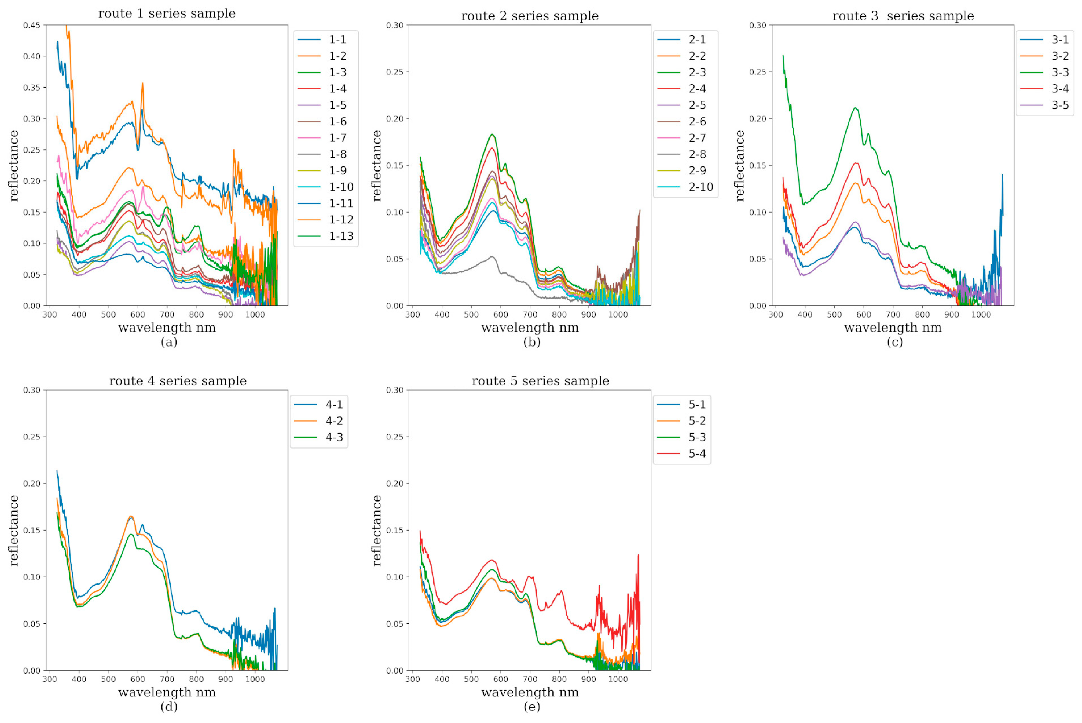
Figure 4 shows the reflectance from in situ collected ASD reflectance on different routes covering the whole study area. The difference in the reflectance of each plot in Figure 4 is not striking, since we repeated the calibration using a standard white panel with a known radiance and a corresponding DN value every time we went to another sample site to collect samples.

Figure 4 shows that the content levels of almost all abovementioned water quality parameters in the route 1 series are relatively higher than those of others. Although there is some noise in Figure 4, the proposed model has an end to end structure, including feature engineering, which denoises the original reflectance, obtaining the feature information (PCA) for projecting the denoised reflectance, and transferring UAV featuring information into ground featuring information. Equation (3) helps to reduce medium interference, as stated in Section 2. The low reflectance values in Figure 4a value may be caused by nitrogen and phosphorus absorption at reflectances near 900 nm [27,40,41]. Additionally, there is a big jump to higher reflectance values around 560 nm and a drop to lower reflectance values around 750 nm followed by a small peak around 800 nm and great jump to higher reflectance values around 900 nm which may be a reason for the high concentration of COD, BOD, and Chla [42,43,44]. Meanwhile, Figure 4b indicates that the wavelengths have similar distributions of reflectance as in Figure 4a and the only apparent difference between them is the fact that reflectance values of Figure 4b are mostly lower than those of Figure 4a near 900 nm, where the content levels of phosphorus, nitrogen, COD, BOD, and Chla, are lower than those of Figure 4a [40]. The low values of Figure 4b can be caused by interference by a flowing and wavy water surface and partial shadow. Figure 4c has similarly lower values of phosphorus, nitrogen, and Chla with Figure 4b for a similar reason [40,41]. The reason for the relatively low values in Figure 4c may be caused by the shadow or the absorption of other materials discharged from factories along river banks [40,41]. Figure 4d has a similar distribution of reflectance with Figure 4c but the concentrations of phosphorus, nitrogen, Chla, and COD are lower than those in Figure 4c. Noteworthily, the content levels of nitrogen, phosphorus, and COD may correspond to wavelengths of 900 nm since Figure 4b–d has a relatively lower peak in reflectance values near 900 nm [45,46]. Figure 4e gives a similar reflectance to Figure 4a, where the content levels of water quality parameters from them are similar as well. Figure 5 shows the reflectance values of samples collected by UAV.

Table 2. Range of water quality parameters of different routes consisting of 35 training data in the study area.

	Substance	Phosphorus (mg/L)	Nitrogen (mg/L)	COD (mg/L)	BOD (mg/L)	Chla (μg/L)
Route
1		0.20–0.57	2.20–4.84	14–24	3.5–6.5	3–13
2		0.16–0.29	0.42–2.45	11–29	3.2–5.8	3–8
3		0.13–0.3	1.03–1.91	13–22	4.0–4.4	1–8
4		0.17–0.29	1.03–1.98	17–20	3.1–4.9	1–3
5		0.24–0.47	3.05–4.31	16–26	4.7–5.8	4–13

shows the range of each of water quality parameters from different routes. As shown in Table 2, same water quality parameters from different routes differ from each other. Some values of water quality parameters are different because some of them are near a working drainage system.

Figure 6 shows the training loss plot over epoch, where loss is defined as RMSE and the epoch is defined as an iteration number. The iterations required to train the proposed model is 3000. The loss of Figure 6a–d remains stable around 1000 training iterations and Figure 6e remains stable at 1500 training iterations. Possible explanations for the comparatively slow convergence of loss in Chla can be demonstrated from two perspectives. On the one hand, some water samples have same content levels of Chla corresponding to difference reflectance values, since the measuring precision of the experimental measuring apparatus is unable to distinguish a subtle difference less than one unit of μg/L. On the other hand, some possible noising bands, which currently cannot be detected, certainly affect the performance of the proposed model.

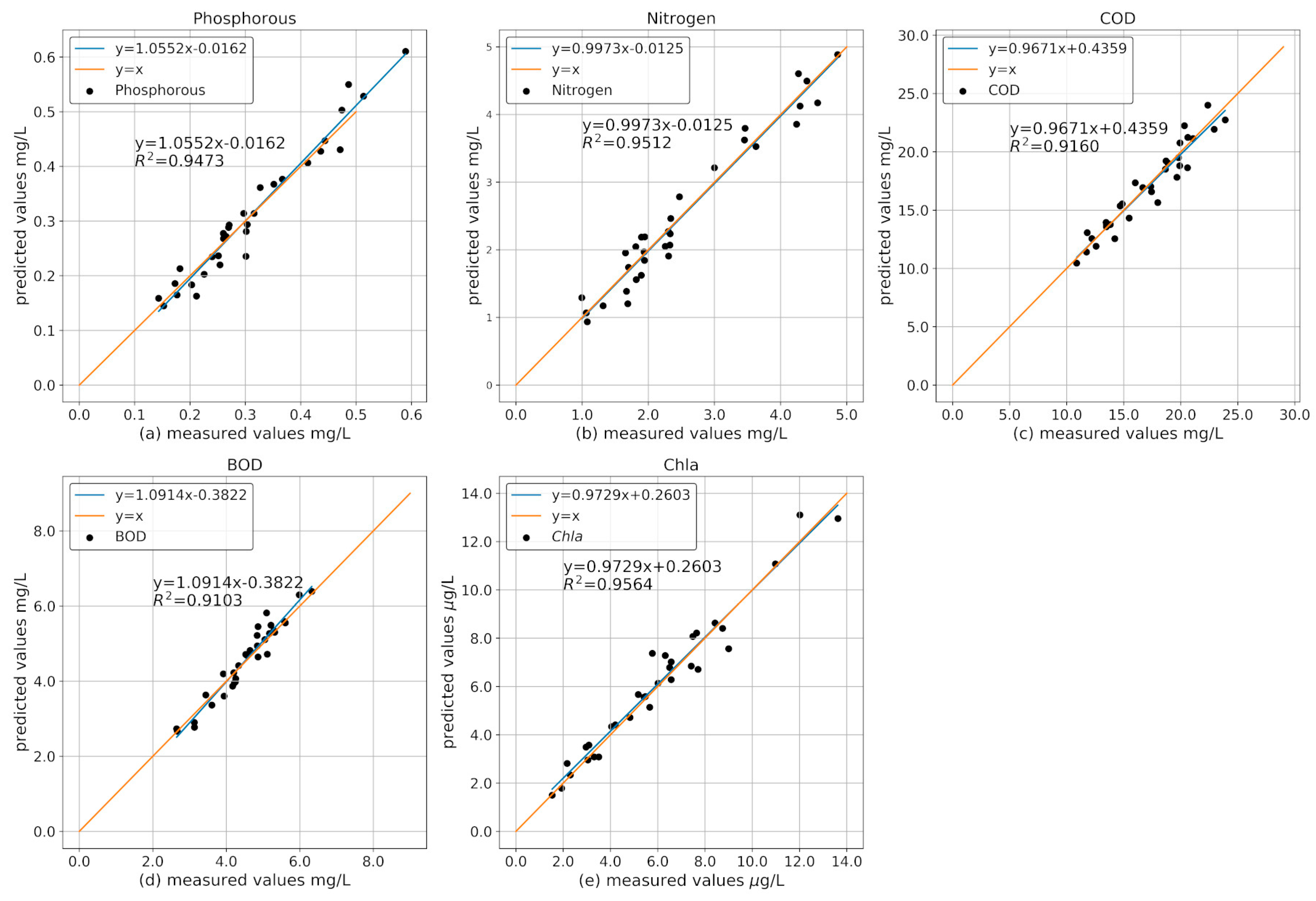
Figure 7 shows the predicted precision of each water quality parameter by comparing predicted values with measured values. The further off the blue line predicted values are, the lower the predicted precision of the proposed model is. The orange line is the regression line between predicted values and measured values. From the goodness-of-fit of the data, nitrogen and Chla obtain the best results. The RSMEs for Figure 7a,b are 0.03, 0.26, 3.15, 0.46, and 0.69, respectively. The MPAE for Figure 7a,b are 8.59%, 3.78%, 8.26%, 7.35%, and 5.43%, respectively.

The water surface band reflectance might suffer uncertainty, which then results in more error in the estimation of water quality estimation. In order to illustrate such an effect, some levels of deviation in the band reflectance are added artificially into the original data. Figure 8 shows a comparison plot of predictions based on different percent deviations in the band reflectance from th perspective of RMSE, given by the proposed hybrid BPNN model. Furthermore, each graph shows that the prediction with 5% deviation from the band reflectance outperforms the others—namely predictions based on the reflectance of 10% and 15% deviations with respect to RMSE. The prediction with 15% deviation from the band reflectance results in the largest error compared to others in each plot. Figure 8 shows that there is a strong relationship between the band reflectance and the concentration of each water quality parameter [27]. It also demonstrates that the more the reflectance deviates from the original band reflectance, the precision explained by RMSE will be lower. Each water quality parameter is calculated using the hybrid BPNN method using the changes in the band reflectance.

This study employed 35 samples collected one day after the collection of the training dataset as the testing dataset. Figure 9 displays the comparison between predicted and ground-measured values from the testing dataset. The proposed method quantitatively predicts phosphorus, nitrogen, COD, BOD, and Chla, clarifying its generality and high accuracy. The accuracy of training results in Figure 7 and Figure 9 is similar, demonstrating that the proposed model is generalized and effective. The mathematical and statistical results of Figure 9 are demonstrated and compared with other models tested on the same dataset in Table 2.

Figure 10 shows the negative ELBO plots of each water quality parameter. As stated earlier in Section 3, we are intended to approximate the real distribution of each weight in hidden layers with a known distribution by minimizing the KL divergence [37]. To minimize the KL divergence between the real distribution of a random variable and the approximate distribution of the same variable, we tried to maximize the ELBO to make our hybrid BPNN model converge where the hybrid BPNN model has been trained 20,000 times to get the best results for ELBO.

Table 3. Comparison of statistical parameters to evaluate different models using hybrid BPNN model, hyperspectral single neural network (NN), and semi-analytical method on the entire area of the Maozhou River.

	Substance	Phosphorus	Nitrogen	COD	BOD	Chla
Statistics
RMSE (hybrid BPNN)		0.03 mg/L	0.28 mg/L	3.28 mg/L	0.49 mg/L	0.75 μg/L
MPAE (hybrid BPNN)		8.97%	4.02%	9.37%	8.73%	6.95%
$R^2$ (hybrid BPNN)		0.95	0.95	0.92	0.91	0.96
RMSE (ANN-BP)		0.09 mg/L	0.43 mg/L	6.25 mg/L	0.74 mg/L	1.41 μg/L
MPAE (ANN-BP)		26.83%	10.34%	16.74%	19.07%	12.53%
$R^2$ (ANN-BP)		0.68	0.78	0.75	0.71	0.70
RMSE (Semi-analytical analysis)		0.10 mg/L	0.57 mg/L	9.39 mg/L	0.95 mg/L	1.96 μg/L
MPAE (Semi-analytical analysis)		45.02%	17.36%	44.77%	23.41%	19.78%
$R^2$ (Semi-analytical analysis)		0.59	0.65	0.61	0.62	0.62
RMSE (empirical regression method)		0.21 mg/L	2.01 mg/L	21.27 mg/L	3.83 mg/L	3.24 μg/L
MPAE (empirical regression method)		51.46%	33.69%	55.37%	58.72%	26.83%
$R^2$ (empirical regression method)		0.53	0.58	0.51	0.49	0.61

shows the performance of different methods on the same testing dataset, including our proposed method, hybrid BPNN, traditional ANN with the backpropagation method [14], a semi-analytical method [11] and an empirical regression method [7,9] on the testing dataset of the whole study area. Our hybrid BPNN method is superior to other methods in terms of RMSE, MPAE and $R^2$. As shown in Table 3, nitrogen predicted by hybrid BPNN obtains the best result for its MPAE, being the lowest, and $R^2$ calculated by hybrid BPNN is the highest compared with other methods. In this research, the importance of MPAE outweighs that of the other two criteria, RMSE and $R^2$, since the numerical magnitude of each water quality parameter differs greatly. More data should be collected from the study area to thoroughly cover a wider numerical range for each water quality parameter so as to improve the prediction precision of water quality parameters. In general, the proposed hybrid BPNN model works effectively for most water quality parameters in the study area.

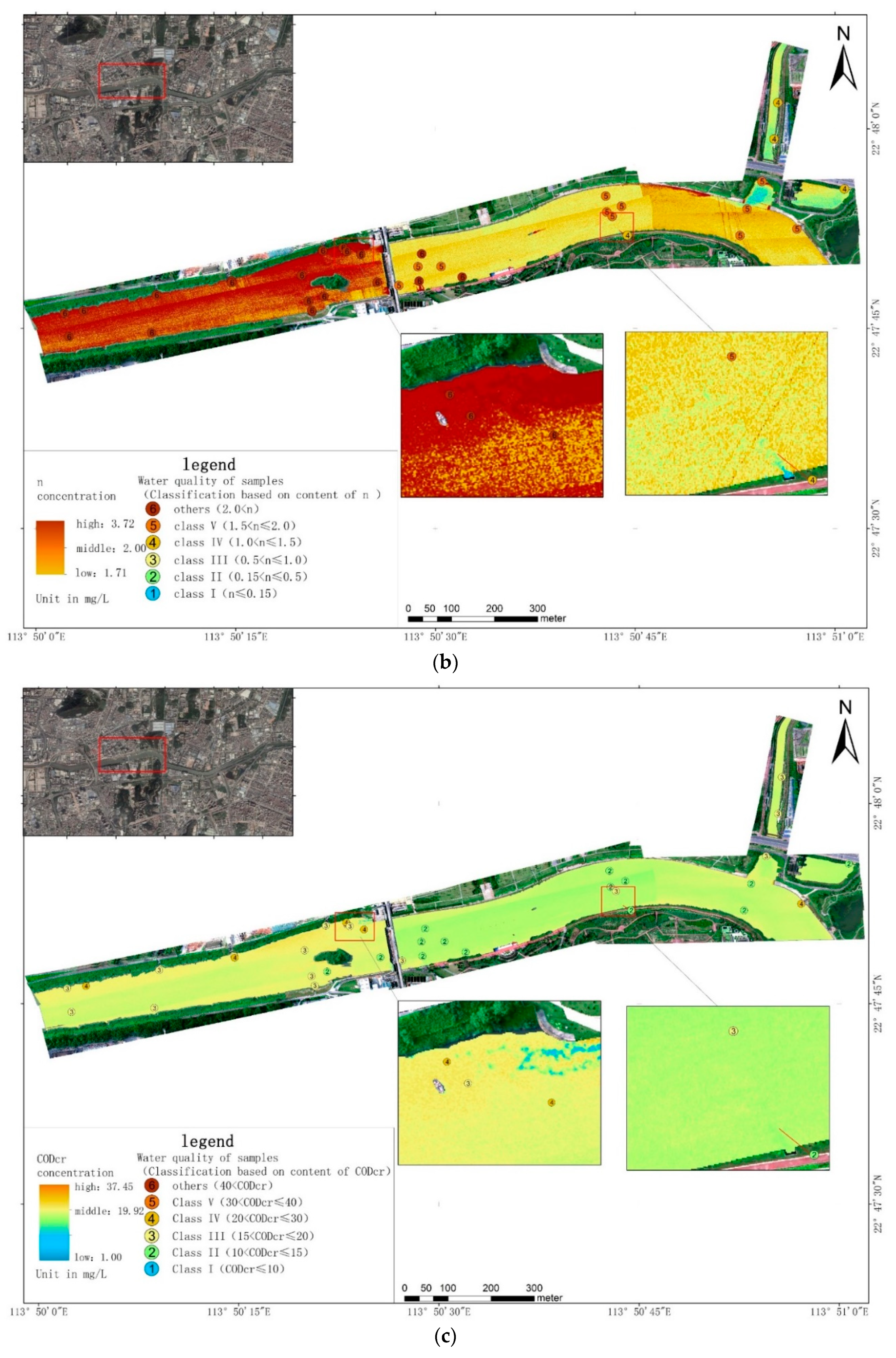
The ground ASD reflectance and numerical concentrations of water quality parameters were used as inputs for the proposed hybrid BPNN model to train the proposed model. UAV hyperspectral image data was transferred to ground ASD reflectance through Equations (2) and (3) in Section 3. Then, the transferred reflectance data from the UAV hyperspectral image can be transformed with eigenvectors, which can be used as inputs for the large-scale numerical prediction of water quality parameters. This study used UAV hyperspectral image data of the entire study area to calculate the concentration of each water quality parameter, as shown in Figure 11, which not only describes the distribution of the content levels of water quality parameters, but categorizes the pollution levels into six levels based on the content levels of each water quality parameter, respectively. Additionally, the criteria of categorization levels conform to the criteria of classification on water quality from our supporting program, Shenzhen Intelligent River pilot program. However, due to restrictions in terms of the UAV flying height and UAV battery imposed by the local government, our UAV had to fly along the river several times, and we had to combine all hyperspectral images to cover the whole study area. Thus, more UAV flights must be implemented to cover the entire study area, since a single flight under these limitations only covers a fraction of the entire study area. The method of data collection by UAV is flexible and effective for scanning reflectance of target object. Combining all UAV hyperspectral images results in combining traces between images in each plot since water is actively flowing, which causes the content level of each water quality parameter to change over time. In this study, UAV has to take several air strips one by one. Figure 11 delineates the resulting distribution of the concentration of water quality parameters at three wavelengths of 480, 550, and 670 nm for RGB color [27]. In Figure 11, the distribution of each water quality parameter can be observed through the change in the color of each plot, and thus local environment protection department can determine the source of pollution according to change in the content levels of each water quality parameter.

5. Discussion

In this study, RMSE, MPAE, and $R^2$ are employed to assess whether the proposed method fits the data appropriately. This study aims to quantify the water quality parameters from a different and novel perspective and shows higher accuracy, interpretability, and computational efficiency with the hybrid Bayesian method, as mentioned in Section 3. Some other methods [12,13,14] predicting the content levels of water quality parameters calculate $R^2$ based on predicted values that are linearly regressed from measured values rather than predicted values from their models, even though they have a relatively high $R^2$ above 0.90. Some multiple piecewise regression methods [10,11] give lower RMSE and higher $R^2$, but they are not generalizable and stable, since $R^2$ values obtained from their methods fluctuate from 0.65 to 0.95 unstably, depending on the type of water quality parameters. The method by Li et al. (2017) used some of the dominant wavelengths where the $R^2$ value is less than 0.8 on average, but this method has less theoretical support and chance discovery plays a large part.

Furthermore, a semi-analytical method matrix inversion method using satellite spectral images as inputs to calculate Chla by Campbell et al. [11] provided changes in MPAE from 8% to 33%, which fluctuated unstably. A CNN regression method for the quantitative estimation of water quality parameters using hyperspectral reflectance bands as inputs to calculate Chla gave an $R^2$ of 0.73 [14] in the training dataset, which randomly assigned 70% of the total dataset as the training dataset and 30% as the testing dataset. In their method, they used six parameters, each consisting of 86 bands from 400 nm to 800 nm, as their input bands, but they did not consider the large-scale calculation of Chla effectively and cost-efficiently since their method only took single point calculation into account. Although these methods obtained relatively good results on their datasets, they did not implement concurrent sampling between ground sampling and satellite image collection, which might incur relatively high bias between training input and futuristic satellite image input for the large-scale calculation of distribution of water quality parameters. A comparison between our proposed method and other methods [9,11,14] shows that our proposed method outperforms others with respect to calculation accuracy (details can be found in Table 3).

Our proposed method is analogous to Bayesian method averaging (BMA), with variable and band selection based on hyperspectral imaging [47]. The BMA method predicted Chla, phosphorus, and nitrogen, with the best results yielding an $R^2$ value over 0.8. It combined experimentally presumed prior and posterior distribution, and then employed a reversible jump Monte Carlo Markov Chain (RJ-MCMC) algorithm to draw random samples of the model as the transient parameters for iterating posterior distribution. Finally, the average of individual predictions in sampled model from the initial state to the current state was calculated by a mathematical equation. Additionally, they evaluated their proposed model through testing if the measured values had confidence intervals, with a significance level of 95% and a paired-t test. The size of the training samples differed with the type of water quality parameters, ranging from 33 to 580, where two thirds of the total dataset worked as training dataset and the rest worked as the testing dataset. The prediction accuracy of their proposed model varied from 0.84 to 0.95 for $R^2$ and from 0.54 mg/m³ to 48.3 mg/L for RMSE depending on which water quality parameter was tested. In a sense, their statistical method for evaluation was not s precisely predicted and measured error-based method since predicted values from their study were not commonly compared with the exact measured values. However, their method was tested if the values were within the confidence interval for evaluate predictive accuracy. Furthermore, their selected bands, with no regard for the size of the dataset, varied with different water quality parameters, causing the computational time to vary considerably. Their BMA method had to be retrained every time new training data were added because one paramount step in BMA, the RJ-MCMC sampler, sampling difficult-to-obtain simulated values for each parameter based on the training dataset, was not able to cope with the accumulated dataset efficiently. Moreover, their band selection method did not consider a situation when they might face a larger dataset; in this case, they would have to re-choose the bands and re-train the model. All of the above studies did not consider medium interference between the satellite and water, which might result in inaccurate spectral measurements and ineffectiveness because medium interference causes higher bias from the real reflectance of water.

In Figure 4, nitrogen and phosphorus may have absorption features in relation to reflectance, ranging from 800 nm to 900 nm, and may have a peak reflectance ranging from 400 nm to 600 nm [27,40,41]. Thus, Figure 4a,e have relatively high content levels of nitrogen and phosphorus. We took ten flights rather than one on the entire study area due to the restriction on UAV flying height imposed by the local government. All hyperspectral images combined from each flight are calculated to show the distribution of water quality parameters across the entire study area, as Figure 11 shows. In Figure 11, we can rationally infer that (a) has a higher concentration of phosphorus near the bank where many local inhabitants pour their living waste, such as washing detergent, remains of farm chemicals, and oil-based substances into the water [48], which is similar to our calculated distribution. The accumulation of phosphorus near the bank is commonly higher than that in areas towards the center of the river. Those are quickly discharged from the bank into the water, causing the instant accumulation of phosphorus, which is carried by the flowing water downstream [49]. Therefore, the aggregation of a high volume of phosphorus always happens near both sides of the bank and phosphorus is unable to move to the center of the river due to the discharge of phosphorus-containing objects and water working as a phosphorus carrier, moving phosphorus-containing objects downstream almost simultaneously. The concentration of phosphorus near the wastewater discharge outlet is higher than that in the neighborhood since water discharged there is mixed with different types of living wastewater. In contrast to the wastewater discharge outlet, the concentration of phosphorus is lower near the purified water discharge outlet. As shown in Figure 11b, the dark red represents a high concentration of nitrogen, which has a similar distribution in Figure 11e since nitrogen is of paramount importance in the synthesis of Chla [50]. The remains of laundry detergent and farm fertilizer are discharged into the river by fishermen and local inhabitants, resulting in an algal boom associated with high concentrations of Chla. The distribution of concentrations of phosphorus can be analogous to that of nitrogen and Chla for some areas along the bank, because nitrogen and phosphorus are vital and indispensable elements in the chemical synthesis of Chla [51,52]. Accordingly, the excess of Chla is associated with the high concentrations of nitrogen and phosphorus. As we observe in Figure 11b,e, some perilous chemical materials such as protoporphyrinogen oxidase (Protox) from herbicide, and copper sulfate used in agriculture or plastic-made materials [53,54], are discharged from the bank of river on the right side of each plot, where the concentrations of nitrogen and of Chla are lower than that on the left side of each plot. Protox is used as a herbicide in agriculture [55] and copper sulfate [56] is beneficial and useful for the agricultural cultivation of aquatic life because it is the main component of algaecides [57] and pesticides used for the prevention of some diseases that commonly occur in aquatic life. Additionally, copper sulfate maintains the agricultural cultivation of aquatic life with regular dosage control [58]. The concentrations of nitrogen and of Chla from the wastewater discharge outlet are lower than those of the purified water discharge outlet in Figure 11b,e. As shown Figure 11c,d, BOD and COD have similar distributions in most areas. According to the previous research provided by the local environment protection department, algae overgrew in the river as large masses of BOD and COD were needed. BOD and COD have higher concentrations near the waste water discharge outlet, but lower concentrations near the purified water discharge outlet because some factories producing leather and paper discharge their industrial waste, including some oxygen-based organic and inorganic matters, into the river through the waste water discharge outlet [59,60]. The concentrations of phosphorus, nitrogen, COD, and Chla are relatively low in the narrower upper watercourse than those in other parts, as shown in Figure 11a,b,d,e, for there are less houses and factories, which have heavy odds in favor of discharging living waste and industrial waste into the river. However, the distribution in the concentration of BOD in Figure 11c is different from that of other water quality parameters in the narrower upper watercourse, mainly because some aquafarms are located along the bank of the narrower upper watercourse where aquatic animals such as fish and plankton are cultivated. Therefore, the concentrations of phosphorus and nitrogen are accordingly lower in narrower upper watercourse since low concentrations phosphorus and nitrogen will restrain the growth of algae. With lower concentrations of phosphorus and nitrogen, algae are deprived of the necessary and essential substances to support their growth, resulting in lower concentrations of Chla [61]. Furthermore, the level of pollution on the left side of each plot with regard to the concentration of each water quality parameter is almost higher than that on the right side, owing to the fact that more factories and residence houses are located along the left bank in each plot. BOD and COD are calculated through the bands ranging from 450 nm to 780 nm [4], which are covered in the range of bands in our research. Nitrogen corresponds to the spectrum ranging from 350 nm to 1100 nm [62,63], phosphorus saliently fluctuates at the spectrum ranging from 400 nm to 900 nm [64], while Chla experimentally responds to the spectrum ranging from 450 nm to 850 nm [38,65]. These water quality parameters are mostly covered within our wavelengths, ranging from 399.69 nm to 1001.08. The accuracy of the methods [8,9] in Table 3 may be relatively low since these methods may not be applicable to some water quality parameters.

However, some limitations exist in this study, such as the limitation of the training data size and the pragmatic bias of the model of transferring UAV reflectance to ASD reflectance. In some other methods [7,8,10,11] with mathematical and experimental analysis, hundreds of samples were employed for the establishment and testing of models, and some water samples are simulated in the laboratory rather than using in situ collected samples. Our water samples are in situ samples, and two factors— the fact that samples are time consuming to collect and expensive to chemically analyze in labs—work heavily against the progress of our research. Additionally, it is hard to quantify water quality parameters based on low-value water reflectance, as the content level of each water quality parameter is comparatively low in Maozhou River. Therefore, the estimation of water quality parameters practically obtains weak signals. Moreover, the small range of content levels for the water quality parameters restrained the variation range of the calculated results, which might influence the calculation accuracy for other areas. The small dataset used to train the model restrained its performance to some extent. The high quality of obtained UAV hyperspectral data should be ensured in order to calculate each water quality parameter with a high accuracy. The featuring bands may not be fixed and deep experiments on the selection of input parameters can be implemented in the future. In accordance with the accumulation of data, our proposed method, hybrid BPNN, will be more generalized and adaptable to hyperspectral data from different areas.

The samples were collected from five different routes, covering the whole study area. Comparatively, the proposed hybrid BPNN model is able to gain better results, outperforming other models [12,13,14] concerned with monitoring water quality parameters based on deep learning. According to previous studies [12,13,14] on the retrieval of quantitative content levels of water quality parameters, pertinent methods for calculating water quality parameters were trained with larger masses of training data and then tested with less data. These methods are comparatively low cost, because the cost of collecting in situ samples is high. Additionally, these methods only work well when a small fraction of the testing data is engaged in testing the model’s performance. When comparing satellite-based hyperspectral remote sensing with other methods, including empirical [7,8], semi-analytical [10,11], and conventional artificial neural network [12,13,14] methods, hyperspectral remote sensing based on UAV through the hybrid BPNN method is more effective because it takes less in situ samples to train the model and it shows a great performance. The results of this study shows that our proposed hybrid BPNN model outperforms other models discussed in Section 4 with respect to $R^2$, RMSE, and MPAE on the same testing dataset, where $R^2$ is over 0.94 and MPAE is less than 10% for all water quality parameters in our study. We do not pay much attention to RMSE, since the numerical magnitude of each water quality parameter differs considerably. The remote sensing methods in other studies are highly expensive, with the lengthy process of retrieving spectral data from a long distance, alongside interferences such as reflection, refraction, and a heterogeneous medium.

In this study, 35 samples were used to train the proposed model due to the constraints of financial support and the time limit. Meanwhile, 35 samples were used to test the model. The utilization of an equal sample size for training and testing models rarely obtains high accuracy and precision. Be that as it may, our proposed model still obtains better results in terms of mathematical and statistical criteria. Our proposed model focuses on the distribution of each parameter, which reduces the limitations of our prior knowledge and makes each parameter follow the practical distributions more flexibly and variationally in order to fit various data. Therefore, the hybrid BPNN model can be trained on less data to obtain greater results. Furthermore, our fitted model works well in our research area, but if different data are collected, our proposed method, hybrid BPNN, will fit other areas as well, since the weight parameters in the Bayesian neural network are sampled from statistical distributions. Thus, this step causes weights to change in order to reduce the loss by increasing ELBO and approximating the real distribution of parameters in hybrid BPNN with more training data employed [37,66,67]. The UAV-transported hyperspectral imager is more cost effective and saves more time compared to satellite-based hyperspectral imagers, with less medium interference. However, satellite-based hyperspectral imagers can cover larger areas, meaning that the hyperspectral images will be high quality where no combining traces exist. Our research will continue, focusing on more hybrid structures of models for the effective assessment of water quality parameters.

6. Conclusions

In this study, the proposed method, hybrid BPNN, is trained on less data but obtains greater results, outperforming other models, as stated earlier, with respect to calculation accuracy, types of water quality parameters, and effectiveness. The proposed method takes featuring reflectance, which it selects through feature engineering, and transfers it from a transferring model, as mentioned in Section 2, to be used as the as input to predict the concentrations of water quality parameters including phosphorus, nitrogen, COD, BOD, and Chla.

Furthermore, our proposed method combines concurrent ground sampling and UAV hyperspectral imaging to reduce the mathematical bias of hyperspectral reflectance and its corresponding content levels of water quality parameters, since the water quality parameters change due to the actively flowing river. Moreover, our proposed method is currently applied to monitor the water quality of Maozhou River, Shenzhen City, Guandong Province, China, based on hyperspectral image data. Thus, the locations of pollution sources can be located through the calculated results.

Further research can be done to reduce the time, labor, and financial cost. Cloud calculation stations can be established to enable a more immediate data exchange. Unmanned boats could be established, so that in situ water samples can be quickly collected and numerically measured for their content. UAV and unmanned boats could be linked through electronic signals to take samples with smaller time differences. The scanning width of a single flight could be wider in order to cover more area and the UAV battery volume could be increased. Thus, this would make it unnecessary to carry out several UAV flights to cover the target area. Moreover, if we carry out less UAV flights, there will be fewer image combining traces caused by the flowing water. Further research may need to consider the application of hybrid BPNN model to other water bodies, and more effort will be made to acquire more pertinent data to make the model structure deeper and more generalized to fit a wider variety of hyperspectral reflectance data.

References

1. Smith, V.H.; Joye, S.B.; Howarth, R.W. Eutrophication of freshwater and marine ecosystems. Limnol. Oceanogr. 2006, 51, 351–355. [Google Scholar] [CrossRef] [Green Version]
2. Kratzer, S.; Kyryliuk, D.; Edman, M.; Philipson, P.; Lyon, S.W. Synergy of Satellite, In Situ and Modelled Data for Addressing the Scarcity of Water Quality Information for Eutrophication Assessment and Monitoring of Swedish Coastal Waters. Remote Sens. 2019, 17, 2051. [Google Scholar] [CrossRef] [Green Version]
3. Ha, N.T.T.; Koike, K.; Nhuan, M.T. Improved Accuracy of Chlorophyll-a Concentration Estimates from MODIS Imagery Using a Two-Band Ratio Algorithm and Geostatistics: As Applied to the Monitoring of Eutrophication Processes over Tien Yen Bay (Northern Vietnam). Remote Sens. 2014, 6, 421–442. [Google Scholar] [CrossRef] [Green Version]
4. Chen, C.; Tang, S.; Pan, Z.; Zhan, H.; Larson, M.; Jönsson, L. Remotely sensed assessment of water quality levels in the Pearl River Estuary, China. Mar. Pollut. Bull. 2007, 54, 1267–1272. [Google Scholar] [CrossRef]
5. Page, B.P.; Olmanson, L.G.; Mishra, D.R. A harmonized image processing workflow using Sentinel-2/MSI and Landsat-8/OLI for mapping water clarity in optically variable lake systems. Remote Sens. Environ. 2019, 231, 111284. [Google Scholar] [CrossRef]
6. Harvey, E.T.; Kratzer, S.; Philipson, P. Satellite-based water quality monitoring for improved spatial and temporal retrieval of chlorophyll-a in coastal waters. Remote Sens. Environ. 2015, 158, 417–430. [Google Scholar] [CrossRef]
7. Gholizadeh, M.H.; Melesse, A.M.; Reddi, L. A comprehensive review on water quality parameters estimation using remote sensing techniques. Sensors 2016, 16, 1298. [Google Scholar] [CrossRef] [Green Version]
8. Li, H.; He, X.; Bai, Y.; Chen, X.; Gong, F.; Zhu, Q.; Hu, Z. Assessment of satellite-based chlorophyll-a retrieval algorithms for high solar zenith angle conditions. J. Appl. Remote Sens. 2017, 11, 012004. [Google Scholar] [CrossRef]
9. Niroumand-Jadidi, M.; Bovolo, F.; Bruzzone, L. Novel Spectra-Derived Features for Empirical Retrieval of Water Quality Parameters: Demonstrations for OLI, MSI, and OLCI Sensors. IEEE Trans. Geosci. Remote Sens. 2019, 99, 1–16. [Google Scholar] [CrossRef]
10. Gurlin, D.; Gitelson, A.A.; Moses, W.J. Remote estimation of chl-a concentration in turbid productive waters—Return to a simple two-band NIR-red model? Remote Sensing Environ. 2011, 115, 3479–3490. [Google Scholar] [CrossRef]
11. Campbell, G.; Phinn, S.R.; Dekker, A.G.; Brando, V.E. Remote sensing of water quality in an Australian tropical freshwater impoundment using matrix inversion and MERIS images. Remote Sens. Environ. 2011, 115, 2402–2414. [Google Scholar] [CrossRef] [Green Version]
12. Chebud, Y.; Naja, G.M.; Rivero, R.G.; Melesse, A.M. Water quality monitoring using remote sensing and an artificial neural network. Water Air Soil Pollut. 2012, 223, 4875–4887. [Google Scholar] [CrossRef]
13. Mohamad, A. Sea water chlorophyll-a estimation using hyperspectral images and supervised Artificial Neural Network. Ecol. Inform. 2014, 24, 60–68. [Google Scholar]
14. Pyo, J.; Duan, H.; Baek, S.; Kim, M.S.; Jeon, T.; Kwon, Y.S.; Lee, H.; Cho, K.H. A convolutional neural network regression for quantifying cyanobacteria using hyperspectral imagery. Remote Sens. Environ. 2019, 233, 111350. [Google Scholar] [CrossRef]
15. Koponen, S.; Pulliainen, J.; Kallio, K.; Hallikainen, M. Lake water quality classification with airborne hyperspectral spectrometer and simulated MERIS data. Remote Sens. Environ. 2002, 79, 51–59. [Google Scholar] [CrossRef]
16. Woerd, H.J.V.D.; Pasterkamp, R. HYDROPT: A fast and flexible method to retrieve chlorophyll-a from multispectral satellite observations of optically complex coastal waters. Remote Sens. Environ. 2008, 112, 1795–1807. [Google Scholar]
17. Bonansea, M.; Rodriguez, M.C.; Pinotti, L.; Ferrero, S. Using multi-temporal Landsat imagery and linear mixed models for assessing water quality parameters in Río Tercero reservoir (Argentina). Remote Sens. Environ. 2015, 158, 28–41. [Google Scholar] [CrossRef]
18. Thiemann, S.; Kaufmann, H. Lake water quality monitoring using hyperspectral airborne data-a semiempirical multisensor and multitemporal approach for the Mecklenburg Lake District, Germany. Remote Sens. Environ. 2002, 81, 228–237. [Google Scholar] [CrossRef]
19. Toming, K.; Kutser, T.; Laas, A.; Sepp, M.; Paavel, B.; Nõges, T. First experiences in mapping lake water quality parameters with Sentinel-2 MSI imagery. Remote Sens. 2016, 8, 640. [Google Scholar] [CrossRef] [Green Version]
20. Qu, Y.; Wang, J.; Wan, H.; Li, X.; Zhou, G. A Bayesian network algorithm for retrieving the characterization of land surface vegetation. Remote Sens. Environ. 2008, 112, 613–622. [Google Scholar] [CrossRef]
21. Eilander, D.; Annor, F.O.; Lannini, L.; Giesen, N.V.D. Remotely Sensed Monitoring of Small Reservoir Dynamics: A Bayesian Approach. Remote Sens. 2014, 6, 1191–1210. [Google Scholar] [CrossRef] [Green Version]
22. Hollstein, A.; Segl, K.; Guanter, L.; Brell, M.; Enesco, M. Ready-to-Use Methods for the Detection of Clouds, Cirrus, Snow, Shadow, Water and Clear Sky Pixels in Sentinel-2 MSI Images. Remote Sens. 2016, 8, 666. [Google Scholar] [CrossRef] [Green Version]
23. Li, T.; Motagh, M.; Wang, M.; Zhang, W.; Gong, C.; Xiong, X.; He, J.; Chen, L.; Liu, J. Earth and Rock-Filled Dam Monitoring by High-Resolution X-Band Interferometry: Gongming Dam Case Study. Remote Sens. 2019, 11, 246. [Google Scholar] [CrossRef] [Green Version]
24. Wu, Q.; Zhou, H.; Tam, N.F.; Tian, Y.; Tan, Y.; Zhou, S.; Li, Q.; Chen, Y.; Leung, J.Y. Contamination, toxicity and speciation of heavy metals in an industrialized urban river: Implications for the dispersal of heavy metals. Mar. Pollut. Bull. 2016, 104, 153–161. [Google Scholar] [CrossRef]
25. Chen, L.; He, Q.; Liu, K.; Li, J.; Jing, C. Downscaling of GRACE-Derived Groundwater Storage Based on the Random Forest Model. Remote Sensing. 2019, 11, 2979. [Google Scholar] [CrossRef] [Green Version]
26. Peddle, D.R.; White, H.P.; Soffer, R.J.; Miller, J.R.; Ledrew, E.F. Reflectance processing of remote sensing spectroradiometer data. Comput. Geosci. 2001, 27, 203–213. [Google Scholar] [CrossRef]
27. Zhang, Y.; Wu, L.; Ren, H.; Liu, Y.; Zheng, Y.; Liu, Y.; Dong, J. Mapping Water Quality Parameters in Urban Rivers from Hyperspectral Images Using a New Self-Adapting Selection of Multiple Artificial Neural Networks. Remote Sens. 2020, 2, 336. [Google Scholar] [CrossRef] [Green Version]
28. Ruddick, K.G.; Voss, K.; Boss, E.; Castagna, A.; Frouin, R.; Gilerson, A.; Hieronymi, M.; Johnson, B.C.; Kuusk, J.; Lee, Z. A review of protocols for fiducial reference measurements of downwelling irradiance for the validation of satellite remote sensing data over water. Remote Sens. 2019, 11, 1742. [Google Scholar] [CrossRef] [Green Version]
29. Wang, M.-H.S.; Wang, L.K.; De Michele, E. BOD Determination, Cleaning Solution Preparation, and Waste Disposal in Laboratories. In Waste Treatment in the Service and Utility Industries; CRC Press: Boca Raton, FL, USA, 2017; pp. 797–808. ISBN 978-1-4200-7237-2. [Google Scholar]
30. Wang, M.-H.S.; Wang, L.K.; De Michele, E. Principles, Procedures, and Heavy Metal Management of Dichromate Reflux Method for COD Determination in Laboratories. In Waste Treatment in the Service and Utility Industries; CRC Press: Boca Raton, FL, USA, 2017; pp. 285–295. ISBN 978-1-4200-7237-2. [Google Scholar]
31. Castle, S.C.; Morrison, C.D.; Barger, N.N. Extraction of chlorophyll a from biological soil crusts: A comparison of solvents for spectrophotometric determination. Soil Biol. Biochem. 2011, 43, 853–856. [Google Scholar] [CrossRef]
32. Qiu, X.; Fang, Z.; Yan, X.; Cheng, W.; Lin, K. Chemical stability and toxicity of nanoscale zero-valent iron in the remediation of chromium-contaminated watershed. Chem. Eng. J. 2013, 220, 61–66. [Google Scholar] [CrossRef]
33. Guimaraes, T.T.; Veronez, M.R.; Koste, E.C.; Gonzaga, L.; Bordin, F.; Inocencio, L.C.; Larocca, A.P.C.; Oliveira, M.Z.D.; Vitti, D.C.; Mauad, F.F. An alternative method of spatial autocorrelation for chlorophyll detection in water bodies using remote sensing. Sustainability 2017, 9, 416. [Google Scholar] [CrossRef] [Green Version]
34. Su, T.C. A study of a matching pixel by pixel (MPP) algorithm to establish an empirical model of water quality mapping, as based on unmanned aerial vehicle (UAV) images. Int. J. Appl. Earth Obs. Geoinf. 2017, 58, 213–224. [Google Scholar] [CrossRef]
35. Zeng, C.; Richardson, M.; King, D.J. The impacts of environmental variables on water reflectance measured using a lightweight unmanned aerial vehicle (UAV)-based spectrometer system. ISPRS J. Photogramm. Remote Sens. 2017, 130, 217–230. [Google Scholar] [CrossRef]
36. Jordan, M.I.; Ghahramani, Z.; Jaakkola, T.S.; Saul, L.K. An introduction to variational methods for graphical models. Mach. Learn. 1999, 37, 183–233. [Google Scholar] [CrossRef]
37. Kucukelbir, A.; Tran, D.; Ranganath, R.; Gelman, A.; Blei, D.M. Automatic differentiation variational inference. J. Mach. Learn. Res. 2017, 18, 430–474. [Google Scholar]
38. Sylvain, J.; Mireille, G. A novel maximum likelihood based method for mapping depth and water quality from hyperspectral remote-sensing data. Remote Sens. Environ. 2014, 147, 121–132. [Google Scholar]
39. Olmanson, L.G.; Brezonik, P.L.; Bauer, M.E. Airborne hyperspectral remote sensing to assess spatial distribution of water quality characteristics in large rivers: The Mississippi River and its tributaries in Minnesota. Remote Sens. Environ. 2013, 130, 254–265. [Google Scholar] [CrossRef]
40. Ramoelo, A.; Skidmore, A.K.; Schlerf, M.; Mathieu, R.; Heitkönig, I.M.A. Water-removed spectra increase the retrieval accuracy when estimating savanna grass nitrogen and phosphorus concentrations. ISPRS J. Photogramm. Remote Sens. 2011, 66, 408–417. [Google Scholar] [CrossRef]
41. Mathew, M.M.; Srinivasa Rao, N.; Mandla, V.R. Development of regression equation to study the Total Nitrogen, Total Phosphorus and Suspended Sediment using remote sensing data in Gujarat and Maharashtra coast of India. J. Coast. Conserv. 2017, 21, 917–927. [Google Scholar] [CrossRef]
42. Liu, X.; Zhang, G.; Sun, G.; Wu, Y.; Chen, Y. Assessment of Lake Water Quality and Eutrophication Risk in an Agricultural Irrigation Area: A Case Study of the Chagan Lake in Northeast China. Water 2019, 11, 2380. [Google Scholar] [CrossRef] [Green Version]
43. Li, X.; Huang, M.; Wang, R. Numerical Simulation of Donghu Lake Hydrodynamics and Water Quality Based on Remote Sensing and MIKE 21. Int. J. Geo-Inf. 2020, 9, 94. [Google Scholar] [CrossRef] [Green Version]
44. Kutser, T.; Paavel, B.; Verpoorter, C.; Ligi, M.; Soomets, T.; Toming, K.; Casal, G. Remote sensing of black lakes and using 810 nm reflectance peak for retrieving water quality parameters of optically complex waters. Remote Sens. Environ. 2016, 8, 497. [Google Scholar] [CrossRef]
45. Dekker, A.; Hoogenboom, H.; Goddijn, L.; Malthus, T. The relation between inherent optical properties and reflectance spectra in turbid inland waters. Remote Sens. Rev. 1997, 15, 59–74. [Google Scholar] [CrossRef]
46. Liew, S.; Choo, C.; Lau, J.; Chan, W.; Dang, T. Monitoring water quality in Singapore reservoirs with hyperspectral remote sensing technology. Water Pract. Technol. 2019, 14, 118–125. [Google Scholar] [CrossRef]
47. Zhao, K.; Wulder, M.A.; Hu, T.; Bright, R.; Wu, Q.; Qin, H.; Li, Y.; Toman, E.; Mallick, B.; Zhang, X.; et al. Detecting change-point, trend, and seasonality in satellite time series data to track abrupt changes and nonlinear dynamics: A Bayesian ensemble algorithm. Remote Sens. Environ. 2019, 232, 111181. [Google Scholar] [CrossRef]
48. Foy, R.H.; Lennox, S.D.; Smith, R.V. Assessing the effectiveness of regulatory controls on farm pollution using chemical and biological indices of water quality and pollution statistics. Water Res. 2001, 35, 3004–3012. [Google Scholar] [CrossRef]
49. Bowes, M.J.; House, W.A.; Hodgkinson, R.A.; Leach, D.V. Phosphorus–discharge hysteresis during storm events along a river catchment: The River Swale, UK. Water Res. 2005, 39, 751–762. [Google Scholar] [CrossRef]
50. Abdel-Moati, M. Industrial dumping impact on oxygen and nitrogen fluxes in Abu Qir Bay, southeastern Mediterranean Sea. Environ. Int. 1997, 23, 349–357. [Google Scholar] [CrossRef]
51. Liu, X.; Lee, Z.; Zhang, Y.; Lin, J.; Shi, K.; Zhou, Y.; Qin, B.; Sun, Z. Remote Sensing of Secchi Depth in Highly Turbid Lake Waters and Its Application with MERIS Data. Remote Sens. 2019, 11, 2226. [Google Scholar] [CrossRef] [Green Version]
52. Löfgren, S.; Boström, B. Interstitial water concentrations of phosphorus, iron and manganese in a shallow, eutrophic Swedish lake—Implications for phosphorus cycling. Water Res. 1989, 23, 1115–1125. [Google Scholar] [CrossRef]
53. Jasper, F.; Quednau, B.; Kortenjann, M.; Johanningmeier, U. Control of cab gene expression in synchronized Chlamydomonas reinhardtii cells. J. Photochem. Photobiol. B Biol. 1991, 11, 139–150. [Google Scholar] [CrossRef]
54. Zhou, W.; Chen, Y.; Zhang, L. Characterization and Synthesis through Fast Phase-Transfer of Oil-Soluble Double-Coordinated Tea-Polyphenols Arsenic. J. Biosci. Med. 2014, 2, 34. [Google Scholar] [CrossRef] [Green Version]
55. Geoffroy, L.; Frankart, C.; Eullaffroy, P. Comparison of different physiological parameter responses in Lemna minor and Scenedesmus obliquus exposed to herbicide flumioxazin. Environ. Pollut. 2004, 131, 233–241. [Google Scholar] [CrossRef]
56. Van Hullebusch, E.; Deluchat, V.; Chazal, P.M.; Baudu, M. Environmental impact of two successive chemical treatments in a small shallow eutrophied lake: Part II. Case of copper sulfate. Environ. Pollut. 2002, 120, 627–634. [Google Scholar] [CrossRef]
57. Ma, J.; Xia, W.; Fu, X.; Ding, L.; Kong, Y.; Zhang, H.; Fu, K. Magnetic flocculation of algae-laden raw water and removal of extracellular organic matter by using composite flocculant of Fe3O4/cationic polyacrylamide. J. Clean. Prod. 2019, 248, 119276. [Google Scholar] [CrossRef]
58. Costas, E.; Lopez-Rodas, V. Copper sulphate and DCMU-herbicide treatments increase asymmetry between sister cells in the toxic cyanobacteria Microcystis aeruginosa: Implications for detecting environmental stress. Water Res. 2016, 40, 2447–2451. [Google Scholar] [CrossRef]
59. Jing, X.; Shao, X.; Cao, C.; Fu, X.; Yan, L. Comparison between the Suomi-NPP Day-Night Band and DMSP-OLS for Correlating Socio-Economic Variables at the Provincial Level in China. Remote Sens. 2016, 8, 17. [Google Scholar] [CrossRef] [Green Version]
60. Leiviskä, T.; Nurmesniemi, H.; Pöykiö, R.; Rämö, J.; Kuokkanen, T.; Pellinen, J. Effect of biological wastewater treatment on the molecular weight distribution of soluble organic compounds and on the reduction of BOD, COD and P in pulp and paper mill effluent. Water Res. 2008, 42, 3952–3960. [Google Scholar] [CrossRef]
61. Yacobi, Y.Z.; Moses, W.J.; Kaganovsky, S.; Sulimani, B.; Leavitt, B.C.; Gitelson, A.A. NIR-red reflectance-based algorithms for chlorophyll-a estimation in mesotrophic inland and coastal waters: Lake Kinneret case study. Water Res. 2011, 45, 2428–2436. [Google Scholar] [CrossRef] [Green Version]
62. Kloiber, S.M.; Brezonik, P.L.; Olmanson, L.G.; Bauer, M.E. A procedure for regional lake water clarity assessment using Landsat multispectral data. Remote Sens. Environ. 2002, 82, 38–47. [Google Scholar] [CrossRef]
63. Wang, S.; Zhuang, Q.; Jin, X.; Yang, Z.; Liu, H. Predicting Soil Organic Carbon and Soil Nitrogen Stocks in Topsoil of Forest Ecosystems in Northeastern China Using Remote Sensing Data. Remote Sens. 2020, 12, 1115. [Google Scholar] [CrossRef] [Green Version]
64. Xiong, J.; Lin, C.; Ma, R.; Cao, Z. Remote Sensing Estimation of Lake Total Phosphorus Concentration Based on MODIS: A Case Study of Lake Hongze. Remote Sens. 2019, 11, 2068. [Google Scholar] [CrossRef] [Green Version]
65. Gitelson, A. The peak near 700 nm on radiance spectra of algae and water: Relationships of its magnitude and position with chlorophyll concentration. Int. J. Remote Sens. 1992, 13, 3367–3373. [Google Scholar] [CrossRef]
66. Malve, O.; Laine, M.; Haario, H.; Kirkkala, T.; Sarvala, J. Bayesian modelling of algal mass occurrences—Using adaptive MCMC methods with a lake water quality model. Environ. Model. Softw. 2007, 22, 966–977. [Google Scholar] [CrossRef]
67. Park, M.-H.; Stenstrom, M.K. Using satellite imagery for stormwater pollution management with Bayesian networks. Water Res. 2006, 40, 3429–3438. [Google Scholar] [CrossRef]
68. Newton, M.A.; Raftery, A.E. Approximate Bayesian inference with the weighted likelihood bootstrap. J. R. Stat. Soc. Ser. B 1994, 56, 3–26. [Google Scholar] [CrossRef]
69. Chua, C.; Goh, A.T.C. A hybrid Bayesian back-propagation neural network approach to multivariate modelling. Int. J. Numer. Anal. Methods Geomech. 2003, 27, 651–667. [Google Scholar] [CrossRef]
70. Friedman, N.; Koller, D. Being Bayesian about network structure. A Bayesian approach to structure discovery in Bayesian networks. Mach. Learn. 2003, 50, 95–125. [Google Scholar] [CrossRef]
71. Polson, N.G.; Sokolov, V. Deep learning: A Bayesian perspective. Bayesian Anal. 2017, 12, 1275–1304. [Google Scholar] [CrossRef]
72. Hutter, M.; Zaffalon, M. Distribution of mutual information from complete and incomplete data. Comput. Stat. Data Anal. 2005, 48, 633–657. [Google Scholar] [CrossRef] [Green Version]
73. Yan, D.; Zhou, Q.; Wang, J.; Zhang, N. Bayesian regularisation neural network based on artificial intelligence optimisation. Int. J. Prod. Res. 2017, 55, 2266–2287. [Google Scholar] [CrossRef]
Figure 1. (a) Maozhou River watershed: the entire Maozhou River from its source (Yangtai Mountain) to its estuary, with its topography. The red rectangle covers the watershed of Maozhou River. (b) Study area of Maozhou River and the location of ground-based measurement. (c) The enlarged area surrounded by the red polygon of Maozhou River. The background images of (b) and of (c) are from Google Earth and Unmanned Aerial Vehicle (UAV) hyperspectral images, with common parts overlapping, respectively. (d,e) The individual flight image, combined with (c); (a,b) are from Google Maps. (ce) are UAV-collected images. UAV and ground data collection will obtain the samples simultaneously at each sampling site in Figure 1b. Analytical spectral device (ASD) data was collected on Aug. 5, 2019, between 9 a.m. and 6 p.m.
Remotesensing 12 01567 g001aRemotesensing 12 01567 g001bRemotesensing 12 01567 g001c
Figure 2. The workflow of estimating water quality parameters by hybrid Bayesian probabilistic neural network (BPNN) model.
Remotesensing 12 01567 g002
Figure 3. The structure of hybrid BPNN.
Remotesensing 12 01567 g003
Figure 4. Water reflectance of different points of the training dataset collected through the routes in Figure 1a by ASD. (ae) represent the reflectance of samples at each wavelength from route 1–5 collected by ASD as described in Figure 1b.
Remotesensing 12 01567 g004
Figure 5. The reflectance values of UAV collected water samples along the same routes in Figure 1. UAV reflectance can be applied to establishment of transferring model as Equation (3). (ae) represent the reflectance of samples at each wavelength from route 1–5 collected by UAV as described in Figure 1b.
Remotesensing 12 01567 g005
Figure 6. The training loss over epoch for proposed hybrid BPNN model. (ae) represent phosphorus, nitrogen, chemical oxygen demand (COD, biochemical oxygen deamand (BOD), and chlorophyll-a (Chla), respectively.
Remotesensing 12 01567 g006
Figure 7. Comparison between the measured and predicted values of water quality parameters in the training dataset. (ae) represent the predicted values from hybrid BPNN model over measured values for phosphorus, nitrogen, COD, BOD, and Chla, respectively.
Remotesensing 12 01567 g007
Figure 8. Comparison of RMSE between the hybrid BPNN models trained with 5%, 10%, and 15% Gaussian random deviation from original reflectance at 3000 training epochs. (ae) represent RMSE comparison plots of the phosphorus, nitrogen, COD, BOD, and Chla with respect to 5%, 10%, and 15% Gaussian random deviation from original reflectance.
Remotesensing 12 01567 g008
Figure 9. Comparison between the measured and predicted values of each water quality parameter in the testing dataset. (ae) represent the predicted values from hybrid BPNN model over measured values for phosphorus, nitrogen, COD, BOD, and Chla, respectively.
Remotesensing 12 01567 g009
Figure 10. Negative evidence lower bound (ELBO) plots of each water quality parameter based on our hybrid BPNN model. (ae) represent the negative ELBO values from hybrid BPNN model over 20,000 iterations for phosphorus, nitrogen, COD, BOD, and Chla, respectively.
Remotesensing 12 01567 g010
Figure 11. Application of the proposed method, hybrid BPNN, in retrieval of water quality parameters. (a) Content level of phosphorus expressed as mg/L. (b) Content level of nitrogen expressed as mg/L. (c) Content level of BOD expressed as mg/L. (d) Content level of COD expressed as mg/L. (e) Content level of Chla expressed as μg/L. Each circle, with its classification number, represents the sampling point in the training dataset. Each number on the right of its adjacent circle represents the route number and predicted value. During the current season, in accordance with the time when the data were collected, the river flowed from right to left in this figure. The left red rectangle represents the waste water discharge outlet. The right red rectangle represents the purified water discharge outlet.
Remotesensing 12 01567 g011aRemotesensing 12 01567 g011bRemotesensing 12 01567 g011c