Quantifying Seagrass Distribution in Coastal Water with Deep Learning Models †

 , , , , ,
Abstract
:1. Introduction
- Can we train a deep learning model to successfully predict the level of LAI based on multispectral satellite images?
- Can we generalize a deep model trained with images from one location to predict seagrass LAI levels at a different location?
- Two deep learning models for regression of seagrass LAI that outperform traditional methods for regression.
- A transfer learning approach that performs seagrass LAI level mapping at a new location with minimum workforce site observation.
2. Related Work
2.1. Deep Learning
2.2. Capsule Networks
2.3. Seagrass LAI Mapping
2.4. Transfer Learning
3. Methodology
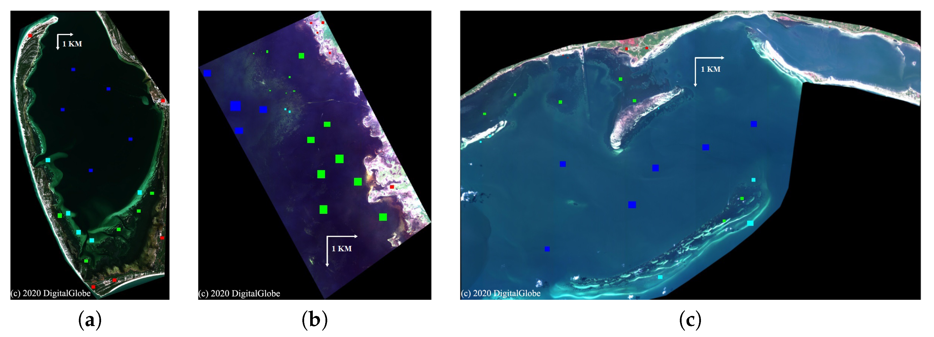
3.1. Datasets
3.2. Data Labeling
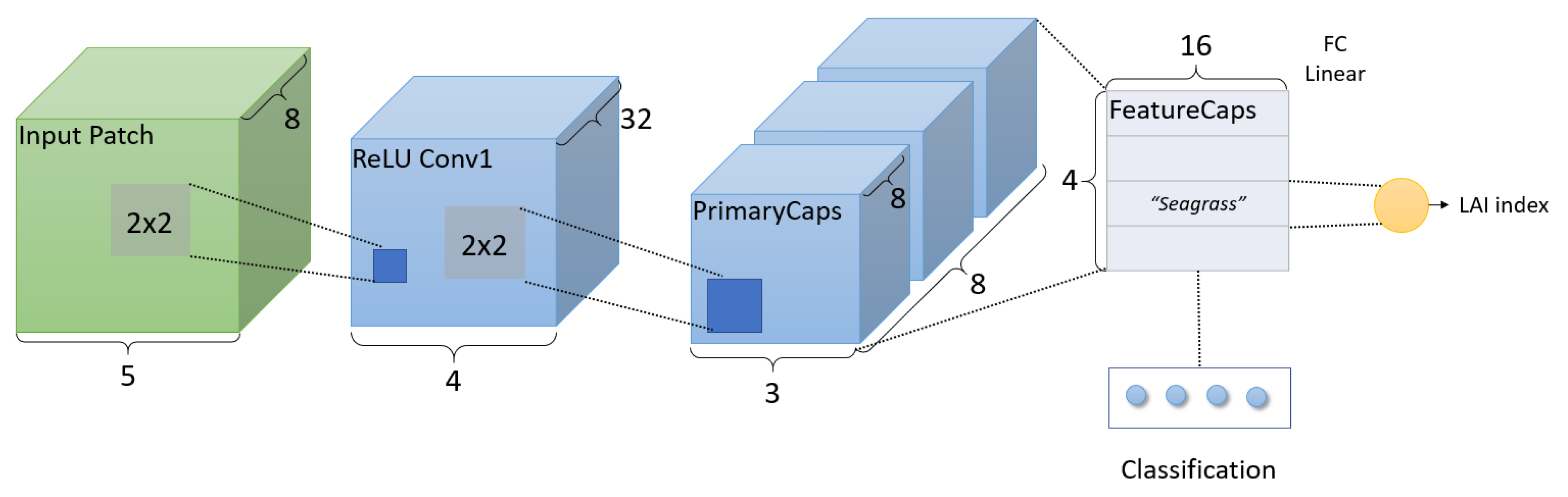
3.3. Joint Optimization of Classification and Regression in Capsule Networks for Seagrass Mapping
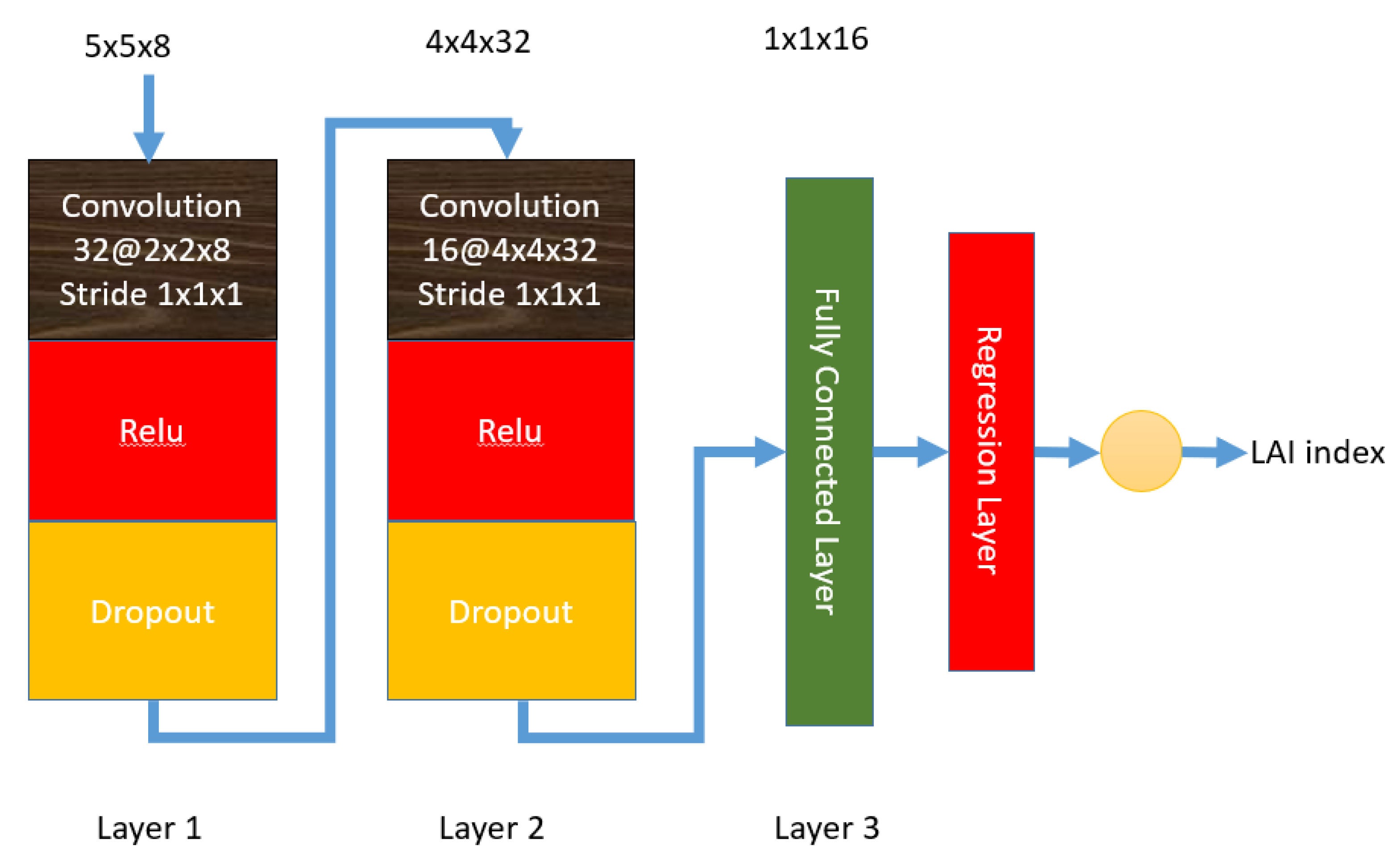
3.4. Convolutional Neural Network for Seagrass Mapping
3.5. Transfer Learning for Seagrass Mapping at Different Locations
- Train a DCN model with all labeled samples from the selected regions in the satellite image taken at St. Joseph Bay (Figure 1a).
- Select a a small portion of the training samples from the satellite image taken at Keeton Beach.
- Classification Step:
- (a)
- Pass the labeled samples through the trained DCN model as shown in Figure 3 and output the 64 features from the FeatureCaps layer as new representations for the labeled samples.
- (b)
- Use the labeled new representations to classify the rest of the unlabeled samples from Keeton Beach using 1-nearest neighbor (1-NN) rule.
- Regression Step:
- (a)
- Use the seagrass vector (16 features) in the labeled new representations from Keeton Beach to train a linear regression model to quantify LAI levels of seagrass.
- (b)
- For every unlabeled patch that is classified as seagrass by the 1-NN rule, predict its LAI value using the linear regression model trained in the previous step. LAI for every non-seagrass patch is set to ‘0.’
- These procedures are repeated for the image taken at St. George Sound for LAI prediction.
4. Experiments and Results
4.1. Model Structure Determination
4.2. Cross-Validation in the Selected Regions
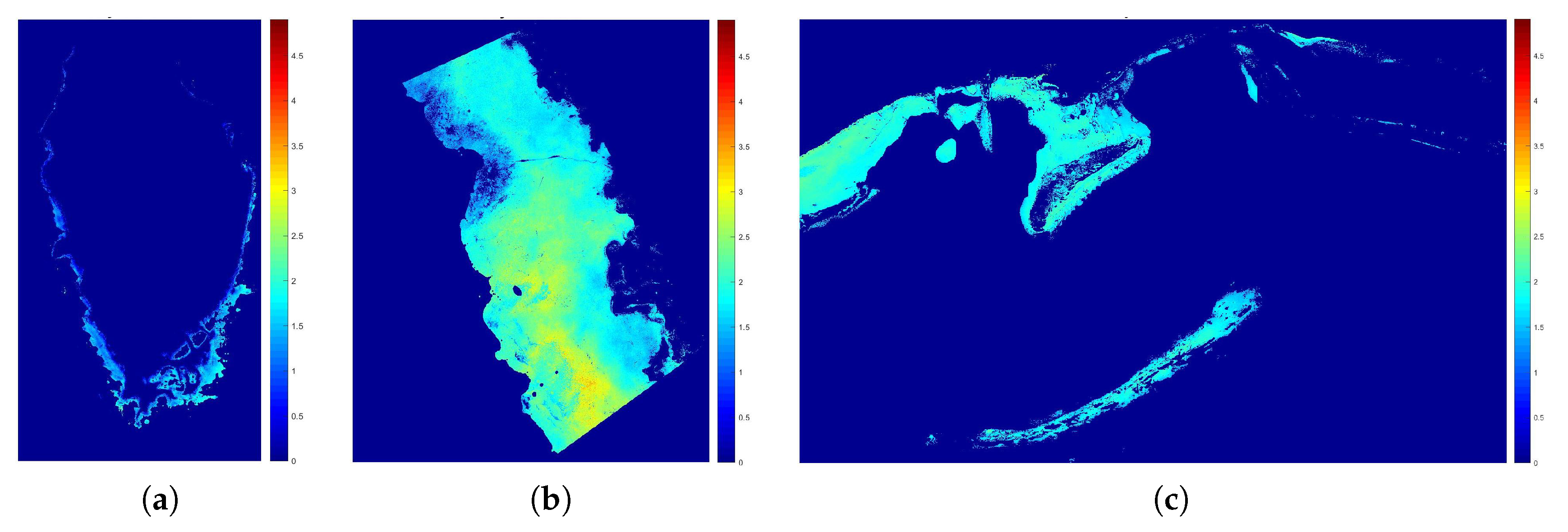
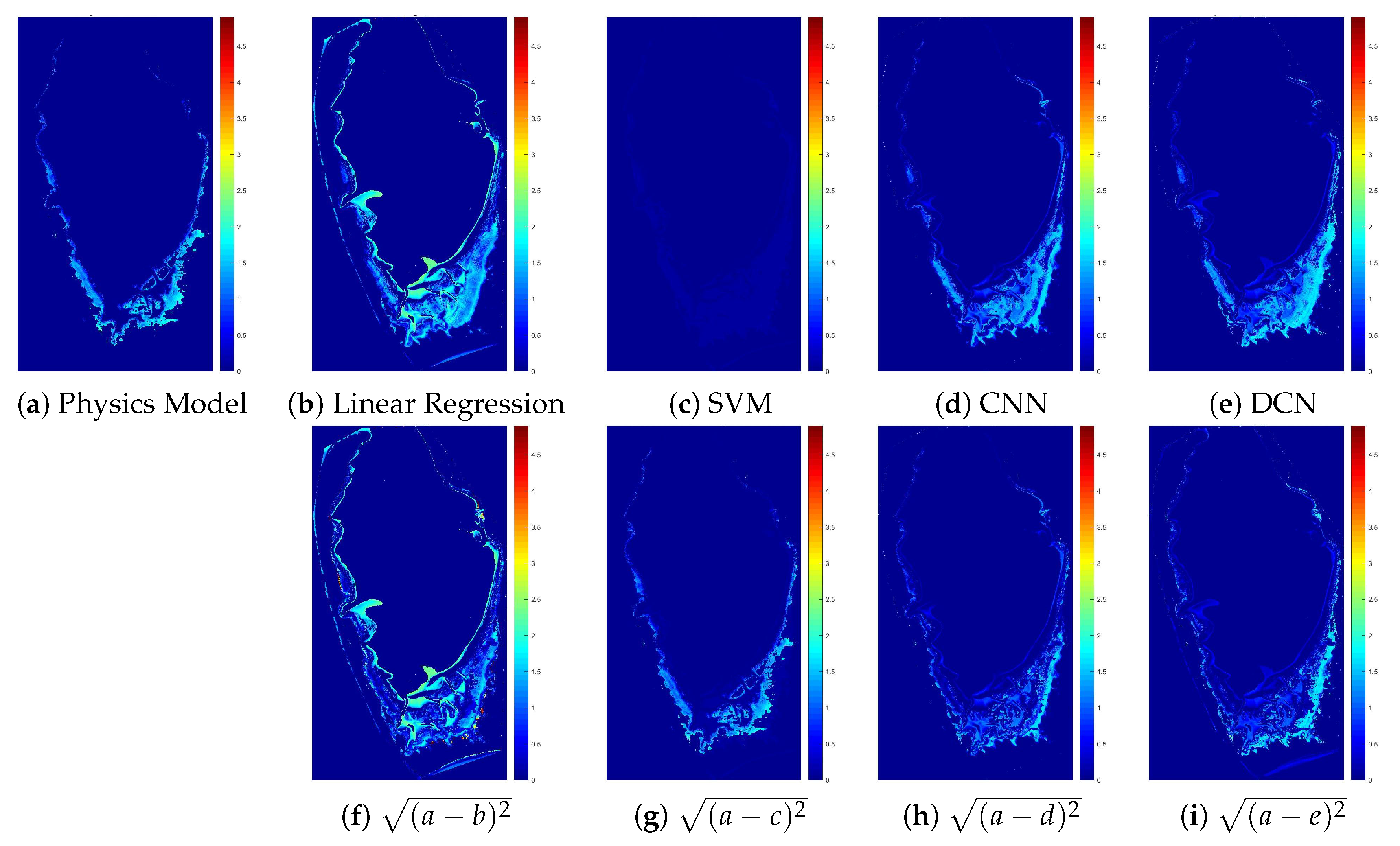
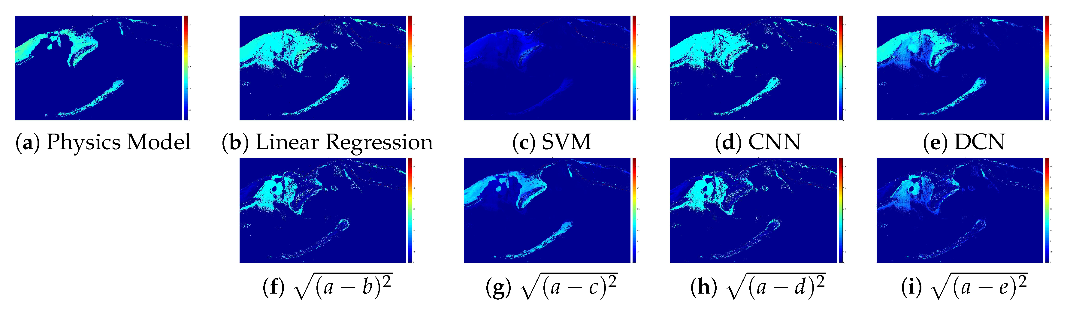
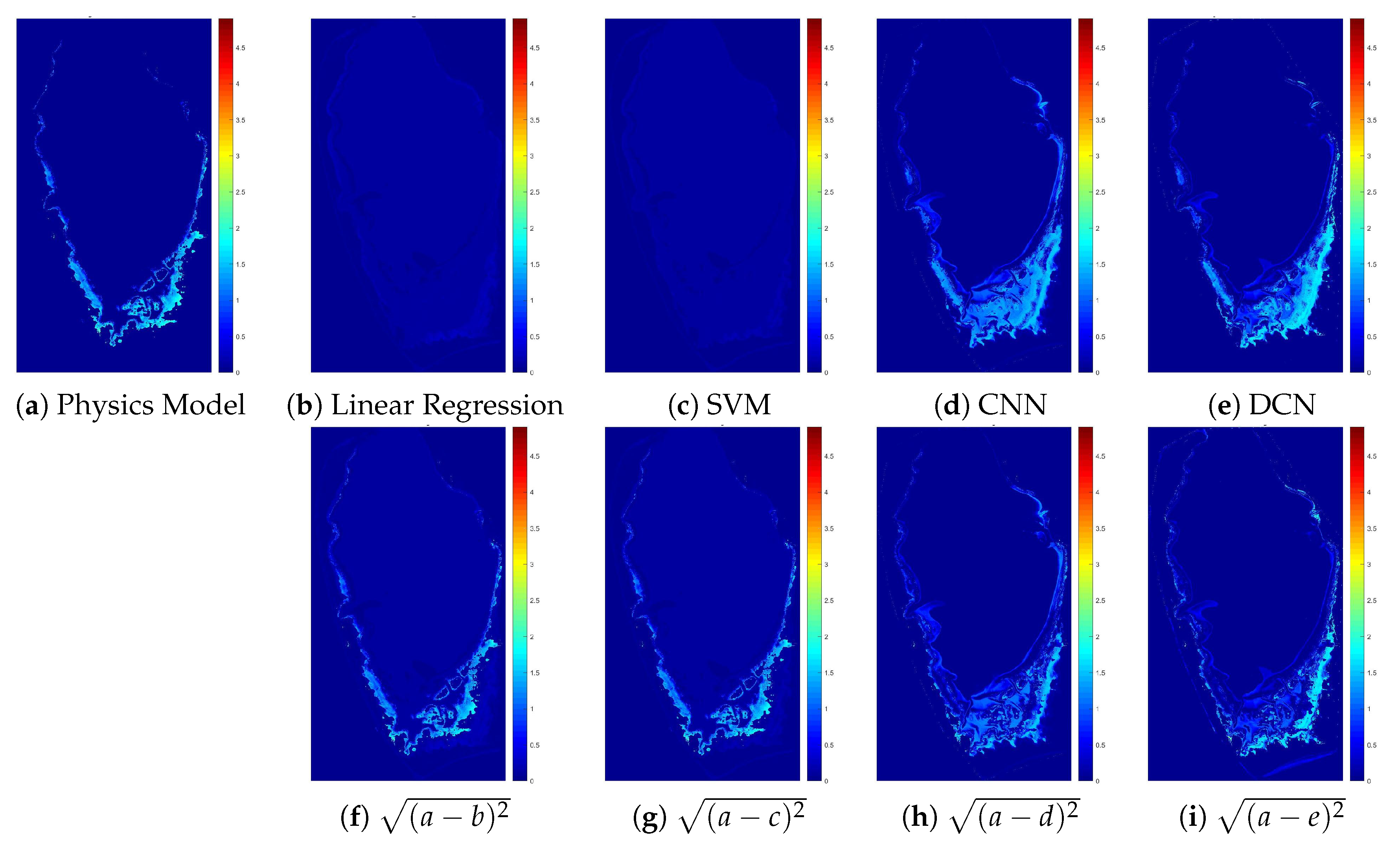
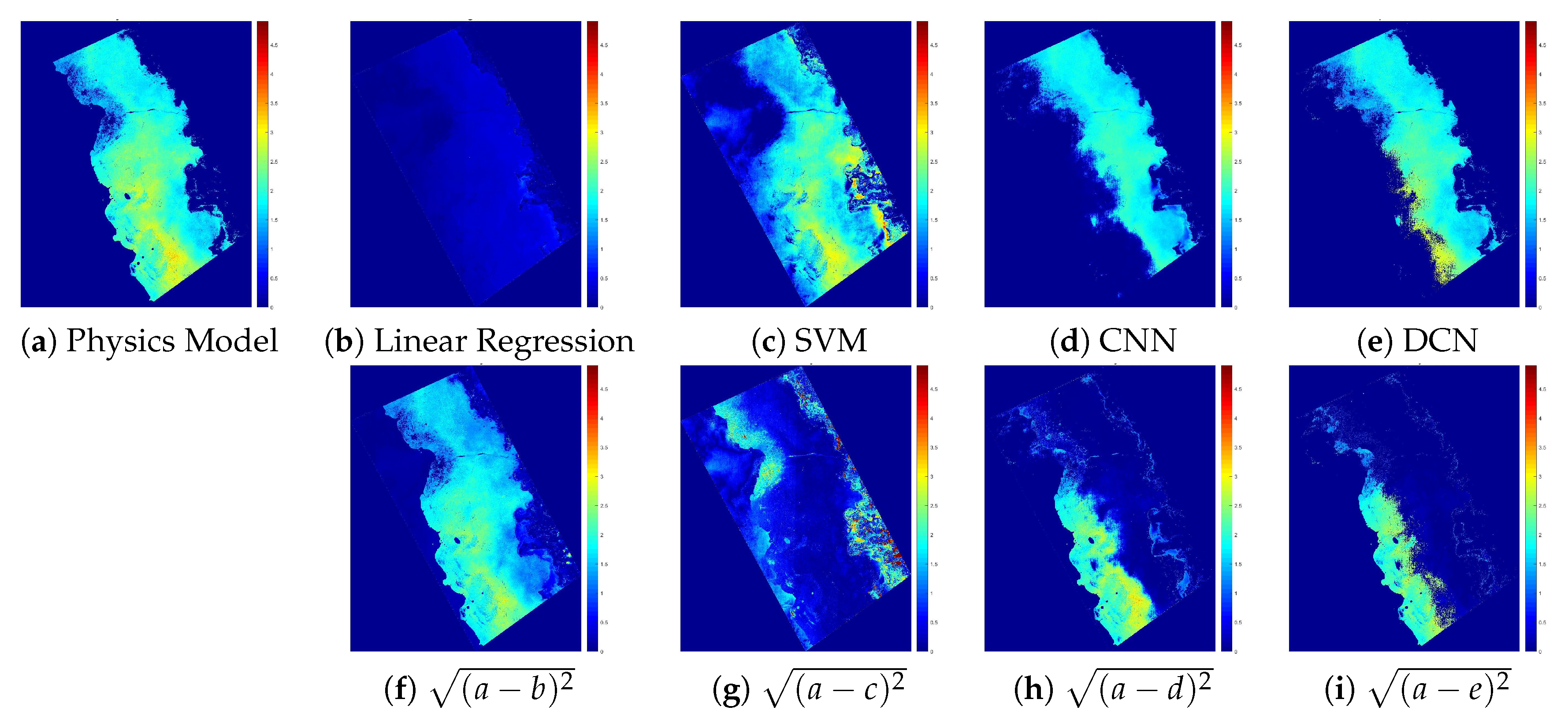
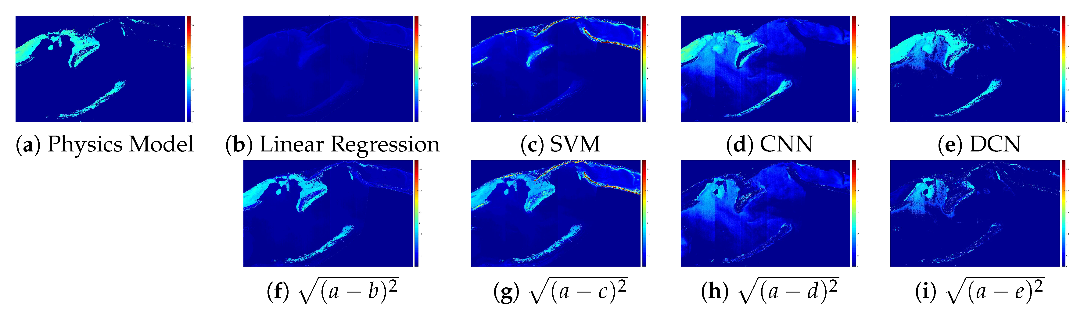
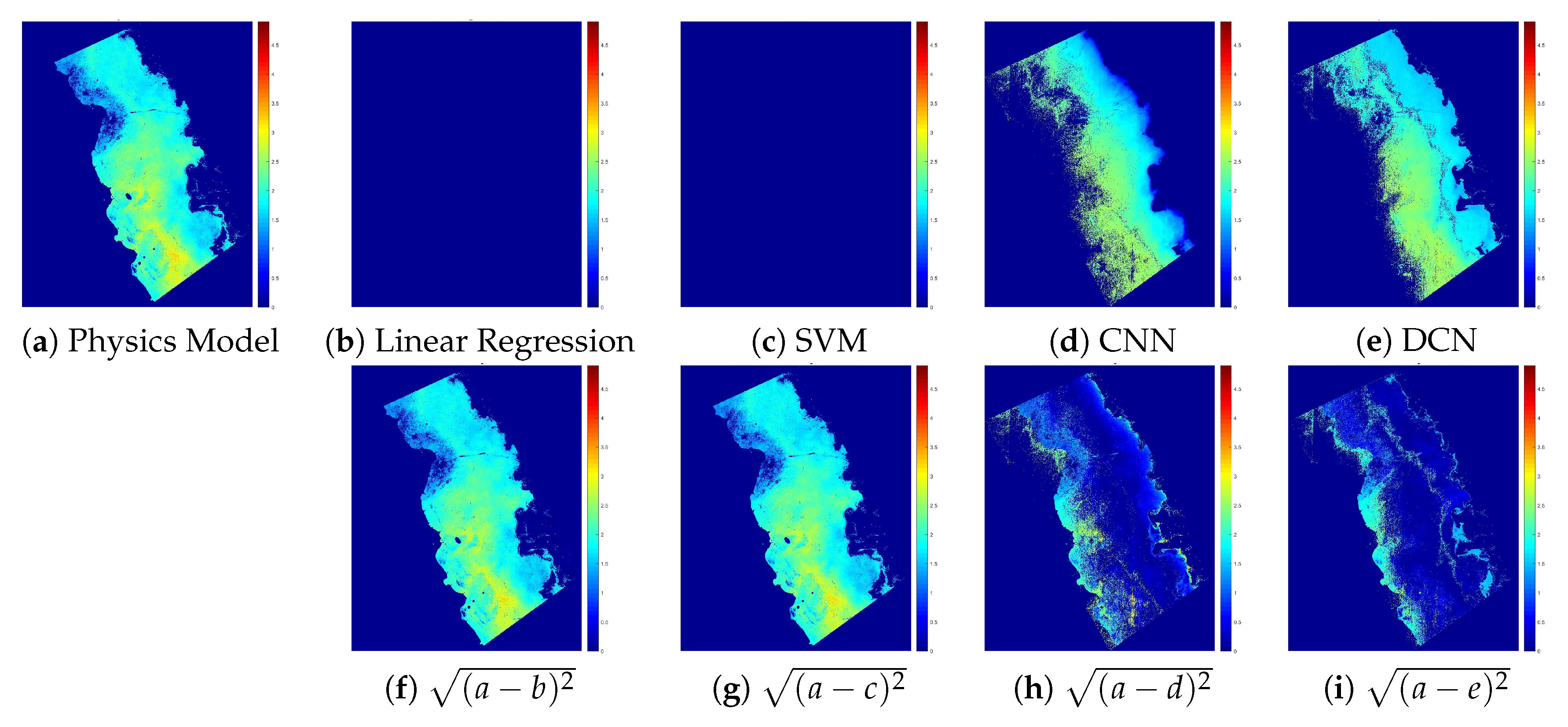
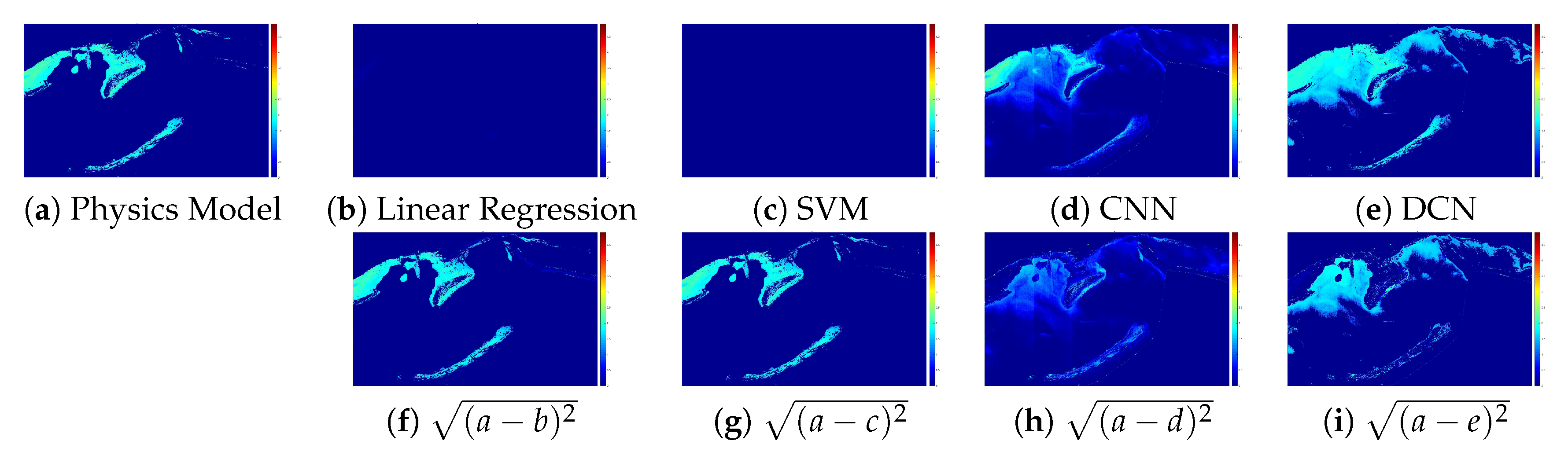
4.3. End-to-End LAI Mapping
4.4. Transfer Learning with Deep Models
4.5. Computational Complexity
5. Discussions
6. Conclusions
Author Contributions
Funding
Conflicts of Interest
References
- Hemminga, M.A.; Duarte, C.M. Seagrass Ecology; Cambridge University Press: Cambridge, UK, 2000. [Google Scholar]
- Wicaksono, P.; Hafizt, M. Mapping seagrass from space: Addressing the complexity of seagrass LAI mapping. Eur. J. Remote Sens. 2013, 46, 18–39. [Google Scholar] [CrossRef]
- Breuer, L.; Freede, H. Leaf Area Index—LAI. 2003. Available online: https://www.staff.uni-giessen.de/~gh1461/plapada/lai/lai.html (accessed on 14 May 2020).
- Hill, V.; Zimmerman, R.; Bissett, W.; Dierssen, H.; Kohler, D. Evaluating light availability, seagrass biomass and productivity using hyperspectral airborne remote sensing in Saint Joseph’s Bay, Florida. Estuaries Coasts 2014, 37, 1467–1489. [Google Scholar] [CrossRef]
- Redmon, J.; Farhadi, A. YOLO9000: Better, faster, stronger. arXiv 2017, arXiv:1612.08242. [Google Scholar]
- Ren, S.; He, K.; Girshick, R.; Sun, J. Faster r-cnn: Towards real-time object detection with region proposal networks. In Proceedings of the Advances in Neural Information Processing Systems, Montreal, QC, Canada, 7–12 December 2015; pp. 91–99. [Google Scholar]
- Lee, H.; Grosse, R.; Ranganath, R.; Ng, A.Y. Convolutional deep belief networks for scalable unsupervised learning of hierarchical representations. In Proceedings of the 26th Annual International Conference on Machine Learning, Montreal, QC, Canada, 14–18 June 2009; pp. 609–616. [Google Scholar]
- Wang, N.; Yeung, D.Y. Learning a deep compact image representation for visual tracking. In Proceedings of the Advances in Neural Information Processing Systems, Lake Tahoe, NV, USA, 5–10 December 2013; pp. 809–817. [Google Scholar]
- Krizhevsky, A.; Sutskever, I.; Hinton, G.E. Imagenet classification with deep convolutional neural networks. In Proceedings of the Advances in Neural Information Processing Systems, Lake Tahoe, NV, USA, 3–6 December 2012; pp. 1097–1105. [Google Scholar]
- He, K.; Zhang, X.; Ren, S.; Sun, J. Deep residual learning for image recognition. In Proceedings of the IEEE Conference on Computer Vision and Pattern Recognition, Las Vegas, NV, USA, 27–30 June 2016; pp. 770–778. [Google Scholar]
- Sermanet, P.; Eigen, D.; Zhang, X.; Mathieu, M.; Fergus, R.; LeCun, Y. Overfeat: Integrated recognition, localization and detection using convolutional networks. arXiv 2013, arXiv:1312.6229. [Google Scholar]
- Perez, D.; Banerjee, D.; Kwan, C.; Dao, M.; Shen, Y.; Koperski, K.; Marchisio, G.; Li, J. Deep learning for effective detection of excavated soil related to illegal tunnel activities. In Proceedings of the IEEE Ubiquitous Computing, Electronics and Mobile Communication Conference, New York, NY, USA, 19–21 October 2017. [Google Scholar]
- Szegedy, C.; Liu, W.; Jia, Y.; Sermanet, P.; Reed, S.; Anguelov, D.; Erhan, D.; Vanhoucke, V.; Rabinovich, A. Going deeper with convolutions. In Proceedings of the IEEE Conference on Computer Vision and Pattern Recognition, Boston, MA, USA, 7–12 June 2015; pp. 1–9. [Google Scholar]
- Oguslu, E.; Islam, K.; Perez, D.; Hill, V.; Bissett, W.; Zimmerman, R.; Li, J. Detection of seagrass scars using sparse coding and morphological filter. Remote Sens. Environ. 2018, 213, 92–103. [Google Scholar] [CrossRef]
- Perez, D.; Lu, Y.; Kwan, C.; Shen, Y.; Koperski, K.; Li, J. Combining Satellite Images with Feature Indices for Improved Change Detection. In Proceedings of the IEEE Ubiquitous Computing, Electronics & Mobile Communication Conference, New York, NY, USA, 8–10 November 2018. [Google Scholar]
- Lu, Y.; Perez, D.; Dao, M.; Kwan, C.; Li, J. Deep Learning with Synthetic Hyperspectral Images for Improved Soil Detection in Multispectral Imagery. In Proceedings of the IEEE Ubiquitous Computing, Electronics & Mobile Communication Conference, New York, NY, USA, 8–10 November 2018; pp. 8–10. [Google Scholar]
- Hoque, M.R.U.; Islam, K.; Perez, D.; Hill, V.; Schaeffer, B.; Zimmerman, R.; Li, J. Seagrass Propeller Scar Detection using Deep Convolutional Neural Network. In Proceedings of the IEEE Ubiquitous Computing, Electronics & Mobile Communication Conference, New York, NY, USA, 8–10 November 2018. [Google Scholar]
- Yang, J.; Zhao, Y.Q.; Chan, J.C.W. Learning and transferring deep joint spectral–spatial features for hyperspectral classification. IEEE Trans. Geosci. Remote Sens. 2017, 55, 4729–4742. [Google Scholar] [CrossRef]
- Hinton, G.; Deng, L.; Yu, D.; Dahl, G.E.; Mohamed, A.R.; Jaitly, N.; Senior, A.; Vanhoucke, V.; Nguyen, P.; Sainath, T.N.; et al. Deep neural networks for acoustic modeling in speech recognition: The shared views of four research groups. IEEE Signal Process. Mag. 2012, 29, 82–97. [Google Scholar] [CrossRef]
- Yu, D.; Deng, L. Automatic Speech Recognition; Springer London limited: London, UK, 2016. [Google Scholar]
- Chen, C.; Seff, A.; Kornhauser, A.; Xiao, J. Deepdriving: Learning affordance for direct perception in autonomous driving. In Proceedings of the 2015 IEEE International Conference on Computer Vision (ICCV), Santiago, Chile, 7–13 December 2015; pp. 2722–2730. [Google Scholar]
- Huval, B.; Wang, T.; Tandon, S.; Kiske, J.; Song, W.; Pazhayampallil, J.; Andriluka, M.; Rajpurkar, P.; Migimatsu, T.; Cheng-Yue, R.; et al. An Empirical Evaluation of Deep Learning on Highway Driving. arXiv 2015, arXiv:1504.01716. [Google Scholar]
- Ning, R.; Wang, C.; Xin, C.; Li, J.; Wu, H. Deepmag: Sniffing mobile apps in magnetic field through deep convolutional neural networks. In Proceedings of the 2018 IEEE International Conference on Pervasive Computing and Communications (PerCom), Athens, Greece, 19–23 March 2018; pp. 1–10. [Google Scholar]
- Chowdhury, M.M.U.; Hammond, F.; Konowicz, G.; Xin, C.; Wu, H.; Li, J. A few-shot deep learning approach for improved intrusion detection. In Proceedings of the 2017 IEEE 8th Annual Ubiquitous Computing, Electronics and Mobile Communication Conference (UEMCON), New York, NY, USA, 19–21 October 2017; pp. 456–462. [Google Scholar]
- Perez, D.; Li, J.; Shen, Y.; Dayanghirang, J.; Wang, S.; Zheng, Z. Deep Learning for Pulmonary Nodule CT Image Retrieval—An Online Assistance System for Novice Radiologists. In Proceedings of the 2017 IEEE International Conference on Data Mining Workshops (ICDMW), New Orleans, LA, USA, 18–21 November 2017; pp. 1112–1121. [Google Scholar]
- Niu, Z.; Zhou, M.; Wang, L.; Gao, X.; Hua, G. Ordinal regression with multiple output cnn for age estimation. In Proceedings of the IEEE Conference on Computer Vision and Pattern Recognition, Las Vegas, NV, USA, 27–30 June 2016; pp. 4920–4928. [Google Scholar]
- Yuan, J.; Ni, B.; Kassim, A.A. Half-CNN: A general framework for whole-image regression. arXiv 2014, arXiv:1412.6885. [Google Scholar]
- Girshick, R. Fast r-cnn. In Proceedings of the IEEE International Conference on Computer Vision, Santiago, Chile, 7–13 December 2015; pp. 1440–1448. [Google Scholar]
- Gidaris, S.; Komodakis, N. Object detection via a multi-region and semantic segmentation-aware cnn model. In Proceedings of the IEEE International Conference on Computer Vision, Santiago, Chile, 7–13 December 2015; pp. 1134–1142. [Google Scholar]
- Li, R.; Zhang, W.; Suk, H.I.; Wang, L.; Li, J.; Shen, D.; Ji, S. Deep learning based imaging data completion for improved brain disease diagnosis. In Proceedings of the International Conference on Medical Image Computing and Computer-Assisted Intervention, Boston, MA, USA, 14–18 September 2014; pp. 305–312. [Google Scholar]
- Sabour, S.; Frosst, N.; Hinton, G.E. Dynamic routing between capsules. In Proceedings of the Advances in Neural Information Processing Systems, Long Beach, CA, USA, 4–9 December 2017; pp. 3857–3867. [Google Scholar]
- Sabour, S.; Frosst, N.; Hinton, G. Matrix capsules with EM routing. In Proceedings of the 6th International Conference on Learning Representations (ICLR), Vancouver, BC, Canada, 30 April–3 May 2018; pp. 1–15. [Google Scholar]
- Xi, E.; Bing, S.; Jin, Y. Capsule Network Performance on Complex Data. arXiv 2017, arXiv:1712.03480. [Google Scholar]
- Afshar, P.; Mohammadi, A.; Plataniotis, K.N. Brain tumor type classification via capsule networks. arXiv 2018, arXiv:1802.10200. [Google Scholar]
- Shen, Y.; Gao, M. Dynamic routing on deep neural network for thoracic disease classification and sensitive area localization. In Proceedings of the International Workshop on Machine Learning in Medical Imaging, Granada, Spain, 16 September 2018; pp. 389–397. [Google Scholar]
- Qiao, K.; Zhang, C.; Wang, L.; Yan, B.; Chen, J.; Zeng, L.; Tong, L. Accurate reconstruction of image stimuli from human fMRI based on the decoding model with capsule network architecture. arXiv 2018, arXiv:1801.00602. [Google Scholar]
- Andersen, P.A. Deep reinforcement learning using capsules in advanced game environments. arXiv 2018, arXiv:1801.09597. [Google Scholar]
- LaLonde, R.; Bagci, U. Capsules for Object Segmentation. arXiv 2018, arXiv:1804.04241. [Google Scholar]
- Islam, K.; Perez, D.; Hill, V.; Schaeffer, B.; Zimmerman, R.; Li, J. Seagrass Detection in Coastal Water through Deep Capsule Networks. In Proceedings of the Chinese Conference on Pattern Recognition and Computer Vision, Guangzhou, China, 23–26 November 2018. [Google Scholar]
- Pérez, D.; Islam, K.; Hill, V.; Zimmerman, R.; Schaeffer, B.; Li, J. Deepcoast: Quantifying seagrass distribution in coastal water through deep capsule networks. In Proceedings of the Chinese Conference on Pattern Recognition and Computer Vision (PRCV), Guangzhou, China, 23–26 November 2018; pp. 404–416. [Google Scholar]
- Phinn, S.; Roelfsema, C.; Dekker, A.; Brando, V.; Anstee, J. Mapping seagrass species, cover and biomass in shallow waters: An assessment of satellite multi-spectral and airborne hyper-spectral imaging systems in Moreton Bay (Australia). Remote Sens. Environ. 2008, 112, 3413–3425. [Google Scholar] [CrossRef]
- Short, F.T.; Coles, R.G. Global Seagrass Research Methods; Elsevier: Amsterdam, The Netherlands, 2001; Volume 33. [Google Scholar]
- Yang, D.; Yang, C. Detection of seagrass distribution changes from 1991 to 2006 in Xincun Bay, Hainan, with satellite remote sensing. Sensors 2009, 9, 830–844. [Google Scholar] [CrossRef]
- Pu, R.; Bell, S.; Meyer, C.; Baggett, L.; Zhao, Y. Mapping and assessing seagrass along the western coast of Florida using Landsat TM and EO-1 ALI/Hyperion imagery. Estuar. Coast. Shelf Sci. 2012, 115, 234–245. [Google Scholar] [CrossRef]
- Dierssen, H.M.; Zimmerman, R.C.; Leathers, R.A.; Downes, T.V.; Davis, C.O. Ocean color remote sensing of seagrass and bathymetry in the Bahamas Banks by high-resolution airborne imagery. Limnol. Oceanogr. 2003, 48, 444–455. [Google Scholar] [CrossRef]
- Pan, S.J.; Yang, Q. A survey on transfer learning. IEEE Trans. Knowl. Data Eng. 2010, 22, 1345–1359. [Google Scholar] [CrossRef]
- Donahue, J.; Jia, Y.; Vinyals, O.; Hoffman, J.; Zhang, N.; Tzeng, E.; Darrell, T. Decaf: A deep convolutional activation feature for generic visual recognition. In Proceedings of the International Conference on Machine Learning, Beijing, China, 21–26 June 2014; pp. 647–655. [Google Scholar]
- Yosinski, J.; Clune, J.; Bengio, Y.; Lipson, H. How transferable are features in deep neural networks? In Proceedings of the Advances in Neural Information Processing Systems, Montreal, QC, Canada, 8–13 December 2014; pp. 3320–3328. [Google Scholar]
- Xie, M.; Jean, N.; Burke, M.; Lobell, D.; Ermon, S. Transfer learning from deep features for remote sensing and poverty mapping. arXiv 2015, arXiv:1510.00098. [Google Scholar]
- Jun, G.; Ghosh, J. An efficient active learning algorithm with knowledge transfer for hyperspectral data analysis. In Proceedings of the 2008 IEEE International Geoscience and Remote Sensing Symposium (IGARSS 2008), Boston, MA, USA, 7–11 July 2008; Volume 1, pp. 1–52. [Google Scholar]
- Hu, F.; Xia, G.S.; Hu, J.; Zhang, L. Transferring deep convolutional neural networks for the scene classification of high-resolution remote sensing imagery. Remote Sens. 2015, 7, 14680–14707. [Google Scholar] [CrossRef] [Green Version]
- Banerjee, D.; Islam, K.; Mei, G.; Xiao, L.; Zhang, G.; Xu, R.; Ji, S.; Li, J. A Deep Transfer Learning Approach for Improved Post-Traumatic Stress Disorder Diagnosis. In Proceedings of the 2017 IEEE International Conference on Data Mining (ICDM), New Orleans, LA, USA, 18–21 November 2017; pp. 11–20. [Google Scholar]
- Li, B.; Shen, C.; Dai, Y.; van den Hengel, A.; He, M. Depth and surface normal estimation from monocular images using regression on deep features and hierarchical CRFs. In Proceedings of the IEEE Conference on Computer Vision and Pattern Recognition, Boston, MA, USA, 7–12 June 2015; pp. 1119–1127. [Google Scholar]


| Label | St. Joseph Bay | Deckle Beach | St. George Sound |
|---|---|---|---|
| Sea | 108,675 | 240,361 | 104,094 |
| Land | 16,304 | 7642 | 23,317 |
| Seagrass | 120,375 | 137,210 | 26,573 |
| Sand | 108,167 | 34,059 | 5914 |
| Image | Linear Regression | SVM | CNN | DCN |
|---|---|---|---|---|
| St. Joseph Bay | 0.58 | 0.57 | 0.45 | 0.46 |
| Keeton Beach | 0.16 | 0.16 | 0.04 | 0.07 |
| St. George Sound | 0.12 | 0.10 | 0.08 | 0.12 |
| Mean | 0.29 | 0.28 | 0.19 | 0.21 |
| Image | Model | 50 Patches | 100 Patches | 500 Patches | 1000 Patches |
|---|---|---|---|---|---|
| Keaton Beach | CNN | 0.9145 ± 0.04 | 0.9514 ± 0.01 | 0.9853 ± 0.003 | 0.9902 ± 0.0007 |
| DCN | 0.9311 ± 0.03 | 0.9676 ± 0.01 | 0.9867 ± 0.002 | 0.9908 ± 0.001 | |
| St. George Sound | CNN | 0.9615 ± 0.007 | 0.9635 ± 0.007 | 0.9761 ± 0.008 | 0.9868 ± 0.005 |
| DCN | 0.9529 ± 0.008 | 0.9721 ± 0.01 | 0.9839 ± 0.002 | 0.9896 ± 0.001 |
| Image | Method | 0 Samples | 50 Samples | 100 Samples | 500 Samples | 1000 Samples | ||||
|---|---|---|---|---|---|---|---|---|---|---|
| Transfer Learning | Fine Tuning | Transfer Learning | Fine Tuning | Transfer Learning | Fine Tuning | Transfer Learning | Fine Tuning | |||
| Keeton Beach | CNN | 2.76 | 0.69 ± 0.19 | 1.35 ± 0.14 | 0.52 ± 0.08 | 1.17 ± 0.297 | 0.28 ± 0.03 | 0.66 ± 0.33 | 0.24 ± 0.007 | 0.91 ± 0.47 |
| DCN | 1.72 | 0.63 ± 0.12 | 1.30 ± 0.14 | 0.46 ± 0.06 | 1.16 ± 0.02 | 0.29 ± 0.02 | 0.73 ± 0.31 | 0.25 ± 0.02 | 0.69 ± 0.03 | |
| LR | – | 1.57 ± 0.003 | 1.61 ± 0.01 | 1.62 ± 0.01 | 1.60 ± 0.01 | |||||
| SVM | – | 1.57 ± 0.003 | 1.62 ± 0.003 | 1.52 ± 0.0007 | 1.62 ± 0.003 | |||||
| St. George Sound | CNN | 0.61 | 0.35 ± 0.03 | 0.14 ± 0.01 | 0.31 ± 0.04 | 0.14 ± 0.005 | 0.23 ± 0.05 | 0.09 ± 0.006 | 0.18 ± 0.03 | 0.09 ± 0.01 |
| DCN | 0.56 | 0.34 ± 0.04 | 0.24 ± 0.03 | 0.25 ± 0.07 | 0.20 ± 0.04 | 0.19 ± 0.008 | 0.11 ± 0.01 | 0.15 ± 0.005 | 0.13 ± 0.03 | |
| LR | – | 0.71 ± 0.01 | 0.73 ± 0.002 | 0.72 ± 0.01 | 0.71 ± 0.01 | |||||
| SVM | – | 0.71 ± 0.0003 | 0.72 ± 0.0002 | 0.73 ± 0.0007 | 0.73 ± 0.0005 | |||||
| Model | Training Time (s/Epoch) | Testing Time (ms/Patch) |
|---|---|---|
| DCN | 85.39 | 0.13 |
| CNN | 13.17 | 0.023 |
© 2020 by the authors. Licensee MDPI, Basel, Switzerland. This article is an open access article distributed under the terms and conditions of the Creative Commons Attribution (CC BY) license (http://creativecommons.org/licenses/by/4.0/).
Share and Cite
Perez, D.; Islam, K.; Hill, V.; Zimmerman, R.; Schaeffer, B.; Shen, Y.; Li, J. Quantifying Seagrass Distribution in Coastal Water with Deep Learning Models. Remote Sens. 2020, 12, 1581. https://0-doi-org.brum.beds.ac.uk/10.3390/rs12101581
Perez D, Islam K, Hill V, Zimmerman R, Schaeffer B, Shen Y, Li J. Quantifying Seagrass Distribution in Coastal Water with Deep Learning Models. Remote Sensing. 2020; 12(10):1581. https://0-doi-org.brum.beds.ac.uk/10.3390/rs12101581
Chicago/Turabian StylePerez, Daniel, Kazi Islam, Victoria Hill, Richard Zimmerman, Blake Schaeffer, Yuzhong Shen, and Jiang Li. 2020. "Quantifying Seagrass Distribution in Coastal Water with Deep Learning Models" Remote Sensing 12, no. 10: 1581. https://0-doi-org.brum.beds.ac.uk/10.3390/rs12101581