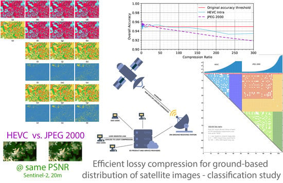
Lossy Compression of Multispectral Satellite Images with Application to Crop Thematic Mapping: A HEVC Comparative Study

Abstract

Remote sensing applications have gained in popularity in recent years, which has resulted in vast amounts of data being produced on a daily basis. Managing and delivering large sets of data becomes extremely difficult and resource demanding for the data vendors, but even more for individual users and third party stakeholders. Hence, research in the field of efficient remote sensing data handling and manipulation has become a very active research topic (from both storage and communication perspectives). Driven by the rapid growth in the volume of optical satellite measurements, in this work we explore the lossy compression technique for multispectral satellite images. We give a comprehensive analysis of the High Efficiency Video Coding (HEVC) still-image intra coding part applied to the multispectral image data. Thereafter, we analyze the impact of the distortions introduced by the HEVC’s intra compression in the general case, as well as in the specific context of crop classification application. Results show that HEVC’s intra coding achieves better trade-off between compression gain and image quality, as compared to standard JPEG 2000 solution. On the other hand, this also reflects in the better performance of the designed pixel-based classifier in the analyzed crop classification task. We show that HEVC can obtain up to 150:1 compression ratio, when observing compression in the context of specific application, without significantly losing on classification performance compared to classifier trained and applied on raw data. In comparison, in order to maintain the same performance, JPEG 2000 allows compression ratio up to 70:1.

1. Introduction and Motivation

Satellite imaging has experienced proliferation in the recent period and there are more possibilities for realization of its applications than ever before. However, data burden is expected to become even greater in the future with the advancement of sensors with higher spatial resolutions and more measurement bands. Therefore, there is a need to revisit and possibly complement some previous findings that were related to efficient satellite image compression, like ones presented in [1], or more recently in [2], and offer users more insights into effects of different choices in such case. Of particular interest is the field of lossy image compression where high compression ratios can be easily achieved, but at the cost of inevitable information loss. However, the question remains what level of image quality degradation could be acceptable for some remote sensing application, and even more importantly, how sensitive such application would be on the particular choice of an image compression strategy. This paper tries to offer some answers to such questions and tracks possibilities of using one of the latest, industry confirmed, general purpose coding standard, which could be expected to be easily accessible to broad community of users, and easy to implement in custom, application dependant, processing frameworks. More exactly, we present a comparative study in which the effectiveness of the intra coding part of the High Efficiency Video Coding (HEVC) standard [3,4] is analyzed against the well established JPEG 2000 lossy compression [5,6], under two selected application scenarios:

(a)

HEVC as a general purpose lossy compression solution for medium and high resolution multispectral satellite images acquired by the Landsat-8’s OLI [7,8], and Sentinel-2’s multispectral instrument (MSI) [9,10], which are considered as frequently used and freely available image sources; and

(b)

HEVC as an application oriented lossy compression solution for thematic mapping, i.e., pixel-based crop classifications like the ones presented in [11,12]—however with an important difference that multispectral time series in our study consist of lossy compressed reflectance measurements as compared to original (uncompressed or lossless) measurements that were used in the referred studies.

The choice of the second application scenario has been influenced by the fact that the corresponding classifier design, and the subsequent production phases, where the trained model is going to be deployed, require large volumes of data. Therefore, such tasks could easily benefit from the effective lossy image compression, resulting in the more efficient data handling. They could also benefit from the possible side effects, like the noise cancelling, leading to the better classifier performance, as in [13,14]. Naturally, this could be only possible if such lossy compression classification approach, usually denoted as compress-then-analyze, would prove to be not highly sensitive to the expected information loss. Thus, the aim of this work is to offer an application oriented insight into specific compression vs. classification performance trade-off in the pixel-based crop classification tasks, through estimation of the corresponding classification performance sensitivity, similarly as in [15]. Also, since we advocate the use of the standardized compression solutions, instead of custom-made codecs that cannot benefit to such extent from the large community support (optimized hardware implementations and continuously maintained software libraries), HEVC effectiveness is tested against the JPEG 2000, which has been often utilized in Earth Observation (EO) data distribution systems.

Besides the possible advantages arising from utilizing the baseline (still-image) HEVC intra mode, we also point out that the particular thematic mapping application that has been chosen in this study represents a sort of typical remote sensing tasks. However, it has not been frequently analyzed from the application perspective of the general data compression community. Moreover, currently there is not so much research on this topic, and a comprehensive analysis of the compression effects on remote sensing applications has been relatively scarce. Therefore, the EO community could benefit from more interest of the compression community for the specific application oriented compression scenarios, as well as from the comprehension of how some finely tuned and well established (off-the-shelf) data compression technique could effect different bands of acquired multispectral images, and to what extent this choice could be expected to have influence on some particular remote sensing application.

Results presented in this paper confirm that HEVC, as a hybrid and feature rich method based on transform and predictive coding techniques, outperforms transform based JPEG 2000 compression approach that has been currently used in some ground-based data distribution systems and has been considered as a general purpose solution for lossless or lossy satellite image compression. The presented results confirm initial assumptions regarding HEVC’s applicability and effectiveness in lossy compression of multispectral images, opening possibly new research directions towards its application in hyperspectral image compression. However, even more importantly, presented results give a new perspective on the possibilities of exploiting general purpose lossy compression solutions, like HEVC, in contemporary ground segment data distribution operations, oriented towards users interested in different levels of quality of service, like in the standard streaming application scenarios.

The rest of the paper is organized as follows. In Section 2, a brief discussion on the current state and future trends in the field of satellite image compression has been given, specifically placing in a given context HEVC as one of the possible compression solution for the future EO data distribution systems. Review of other related coding techniques has been given in the same section. In the Section 3, the underlying data, used as part of experiments, has been briefly described and motivated. Experimental setup and methods used in this study are explained in Section 4. It includes the design characteristics of the crop classification method, that is used as an example of application oriented benchmark in this work, as well as settings of the codecs used for the compression purpose. The results, and additional discussions of the outcomes of this study, are emphasized in Section 5. Presented results in this work include both quantitative and qualitative assessments of compression effects on the image quality, as well as on the overall accuracy of the considered crop thematic maps. The paper is concluded in Section 6, with a short reference to the possible future research directions.

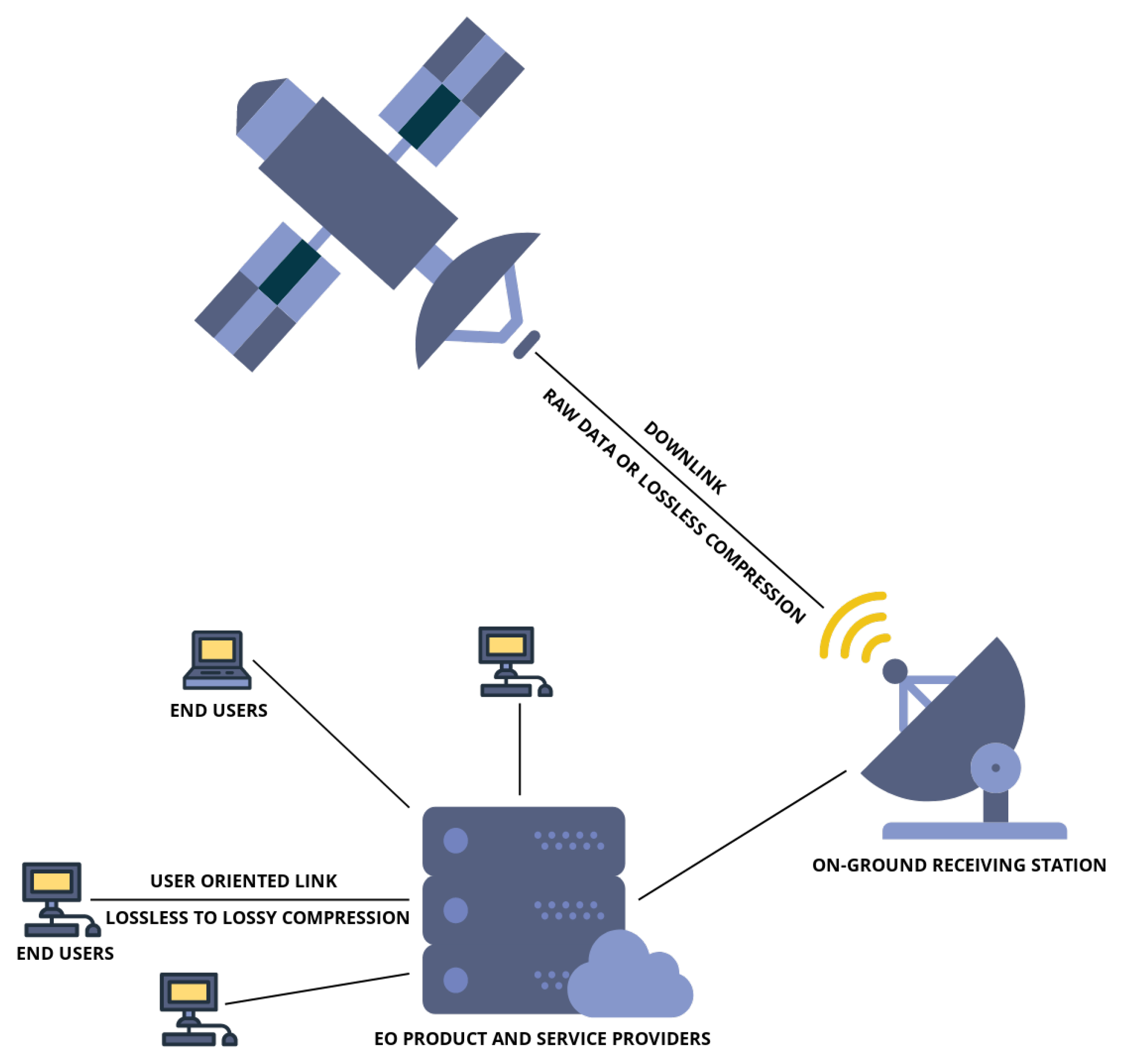
2. Provisioning of EO Data Through Lossy Compression Schemes in the Ground Segment

Broadly speaking, utility of an image compression scheme is mostly affected by the type of data and planned application. Essentially it goes down to the amount of useful information inherent in the data, as compared to the overall data quantity [16], sometimes requiring a global, mission specific approach in a quest for an optimal compression trade-off [17].

2.1. Downlink Related Work

Downlink systems, Figure 1, usually prefer lossless or near-lossless image coding designed in such a way to ensure high fidelity of possible applications. Due to a limited on-board power capacity, low complexity compression schemes, e.g., [18,19,20,21,22,23,24], have been the main choice towards the practical implementation. For example, in such restricted environment, even JPEG 2000 has been considered a too complex method. Consequently, the Consultative Committee for Space Data Systems (CCSDS) has been constituted to research on a family of recommended compression schemes specifically designed for space data systems. Works like these [25,26,27] developed by CCSDS have emerged, following a general paradigm of low complexity requirements in order to facilitate applications such as on-board compression. Aforementioned approaches are just some of the wide range of different coding choices that meet requirements imposed by power-constrained EO missions, with a limited hardware resources specifically designed to function in orbit. However, those techniques are often used with compression ratios that could be considered as moderate [28], sometimes also due to the the nature of the lossless compression itself. Nevertheless, limited bandwidths and ever-growing data volumes make these methods inevitable in today’s EO missions. As a consequence of the huge increment in the data-rate of the new generation sensors (despite that the lossless or near-lossless compression algorithms have been traditionally preferred for on-board compression scenarios), a research effort targeting lossy on-board compression has been reported in [29,30]. Also, lossy extensions of CCSDS standards have been proposed [26,31], however still bearing in mind available on-board technologies related with tolerance to solar radiation and low power consumption, e.g., see [32]. As a matter of fact, it is generally accepted that the lossy coding schemes can be (if required) derived from the corresponding lossless modes through introduction of a suitable quantization (or coefficient truncation) scheme [31,33].

2.2. Focusing towards the Users Side Compression

As opposed to the constraints related to the on-board processing and downlink communication requirements, end-user oriented EO applications, that are placed at the other end of the data distribution chain, offer much broader range of design possibilities. Liberating from the tendency to suggest low-power codec solutions, and approaching closer to end-users, different compression options may appear, especially considering theoretically unlimited resources in the cloud where complexity is no longer a critical issue during the encoding step. Thus, low-complexity requirement imposed over on-board solutions can be significantly relaxed, which can be particularly suited for a more complex compression algorithms that are trying to achieve better trade-off between image quality and compression ratio.

Traditionally, those methods are mainly based on various decorrelating transforms [34,35], leading to wide range of different coding approaches, where usual precondition for efficiently going below the nominal entropy rate of the source is to decorrelate acquired measurements in spatial and/or spectral domain. In particular, general purpose coding schemes, originally designed to be applicable in broader progressive lossless-to-lossy use-case scenarios, such as EZW [36], SPIHT [37,38,39] or SPECK [40,41], proved to be useful in achieving higher compression ratio requirements, however bringing in higher processing and memory requirements when compared to less complex on-board solutions (see Section 2.1). Aforementioned research has established that, among transform coding architectures, many systems usually follow a general coding pipeline in which, at the first stage, a suitable transform is applied in the spectral domain (e.g., wavelets or some covariance-based decorrelation method like Karhunen-Loève transform (KLT) [42] or its low-complexity approximation named Pairwise Orthogonal Transform [43,44]), which is afterwards followed by some of the standard coding schemes (EZW, SPIHT, SPECK). Similarly, JPEG 2000 can be deployed in order to compress each of the previously computed, spectrally decorrelated, image components (usually by implicitly performing an additional 2D spatial transform on each of resulting channels from the first step, followed by rate or quality allocator, and entropy coder), leading to three-dimensional (3-D) decorrelation [13,35,45,46]. In particular, a combination of spectral decorrelator such as KLT in conjunction with JPEG 2000 proved to provide state-of-the-art performance according to [13,43]. Other noteworthy research efforts are also reported in [47,48,49,50].

In addition, authors note that very few works utilize standard video coding schemes, or any similar hybrid-based approaches (combination of predictive coding and transform coding), as a compression choices for high-dimensional satellite data. More precisely, we found out only work presented in [51] worth mentioning. However it does not use HEVC as a base codec setting.

2.3. Applications Oriented Lossy Compression—Related Work

Although higher compression gains may be achieved using lossy compression, there is always a question to what extent some artifacts introduced by the specific compression algorithm affect a certain type of application. Some previous works, that provide insights into this important question, and which could be considered as closely related in the context of the presented study, are given in [15,52,53,54,55]. In [15], as well as [56], it was shown that a small amount of lossy compression can have beneficial effects for the overall performance of crop thematic mapping. This was also independently confirmed by the experimental results of our study. However, in comparison to [15], we have considered different types of compression methods and application scenarios. On the other hand, regarding the specific task of crop thematic mapping, in comparison to [15] our study considers only a multitemporal classification scenario, which can be considered as a more realistic one, as opposed to a single-date classification approach, since it is well known that the plant’s phenology is captured much better by independent observations made throughout the vegetation season. Also, according to [15], multitemporal information allows one to utilize much higher compression ratios in comparison to single-date classification, and still achieve almost the same classification performance as in the case of original data. One of the main conclusions in [52] was that the level of scene fragmentation determines the acceptable level of lossy compression, which is consistent with the general rule of thumb that image’s scene complexity determines the overall information content (entropy of the image), and thus level of required spatial details for successful, discirminative classification. Related to the mentioned fragmentation aspect, scene content complexity was also considered by the first set of experiments in our study, which involves algorithms benchmarking against satellite images with the varying scene content, captured at the approximately same time by the image sensors with varying spatial and spectral characteristics. In addition, influence of lossy compression on the quality of different vegetation indices, which also represent potentially valuable features for crop classification, was analyzed in [53,54]. Favoring image channels that contain more task specific information was also proposed in [54], where the group of channels characteristic for vegetation was encoded at a higher bit rate than the remaining one.

Besides the above mentioned methods, there were also many others which have evaluated compression efficiency against the specific remote sensing tasks like classification [35,43,55,57,58,59,60], image segmentation [61], atmospheric parameter retrieval [14,62], spectral unmixing [63], endmember extraction [64], vegetation [53,54] and spectral [65] indices computation, and biophysical variables estimation [66]. In [59] it was concluded that in the context of the general applications it is hard to define optimal level of image quality that should be preserved by the lossy compression. As a possible answer to this open question, authors in [59] have proposed a general, unsupervised classification-accuracy based method for image quality assessment, which could provide some indicators regarding effectiveness of different elements of the considered compression procedures. In [59] it was also pointed out that the spectral decorrelation usually removes peaks from spectral signatures of hyperspectral measurements, even at high reconstructed image qualities. On the other hand, Ref. [60] proposed a specific classification oriented lossy compression approach, inspired by optimal signal representation in the spectral domain. This approach was later extended in [67]. An overview of the contemporary approaches for measuring how classification accuracy is affected by the compression can also be found in a recent study in [68]. In addition, they establish a prediction model between the features extracted from compressed images and the corresponding classification accuracy.

2.4. HEVC as a Matter of Choice

Generally speaking, role of an efficient compression scheme would be to enable and facilitate deployment of other technologies that are expected to be highly dependant on the efficient and timely distribution of image data, and which would possible benefit from the achieved reduction in the required storage, energy consumption, data access and processing time. This could prove to be extremely important for data vendors, but even more so for individual users, on-demand service providers, or third party stakeholders in general. At the same time, positioning at the ground segment could open the access to the larger compression community that could also be crucial for the implementation of new forms of compression techniques that at the time being have not been considered in the RS applications, e.g., HEVC. In that sense, this work aims to position itself on the link between the EO data service providers and the end-users, see Figure 1. Also, in the context of this work, we consider classification task just as one of the possible user specific applications that could benefit from the reduced data burden that is easily achieved by the lossy compression of multispectral satellite images. In addition, as the remote sensing technologies advance, new applications require constant improvement of existing coding schemes, allowing higher compression gains, which usually (however not necessarily) comes at the price of higher complexity.

Eventually, it is important to note that widely accepted industry standards for image and video compression could ensure interoperability and can be adopted by the broader community of EO practitioners. At the same time, it is more likely to be implemented in a custom, application dependant, processing framework, since they usually come with the open source reference software, e.g., [69]. This implies that efficient, fast and reliable implementation of the standardized codecs may be realized with much less effort than implementing custom based codec from the ground. By doing so, schemes such as HEVC may be deployed efficiently, making available to process large amount of data utilizing computationally complex features like those incorporated in HEVC. Hence, building compression processing unit, on cloud or locally on a workstation (or even personal computer), is significantly facilitated since available computing power comes at reasonable cost. Efficient widely used and industry accepted compression techniques are therefore easier to be integrated in the existing infrastructure, or implemented using existing equipment. In addition, even though HEVC has high computational complexity, it is highly parallelizable and implementation friendly scheme [70,71] (it uses integer logic with shifts and additions). For example, work that implements fast and efficient HEVC encoder was described in [72].

Emerging from the above, in our research, we consider the use of standardized and ubiquitous, industry accepted solution such as HEVC. Technical specifications for the data distribution and management of the most spaceborne programs has identified JPEG 2000 as a straightforward compression solution, e.g., [73]. In this work we want to show that more recent, state-of-the-art standardized compression schemes may provide performance improvement compared to the JPEG 2000. Given the current computing technologies, besides HEVC’s higher computational complexity, it is practically feasible to use such scheme in a ground-based satellite data distribution chain. Hence, we have done comparative study in which we analyze effectiveness of the HEVC standard. We show that using intra-band (still-image) coding part of HEVC can improve compression gain over the JPEG 2000 coding scheme which is specified as a baseline (and mostly used) compression method for EO data distribution at the ground segment. Indeed, HEVC has been reported to perform better than any other international standardized coding scheme currently on the market. It was reported in [74] that HEVC intra coding reduced the average bit rate by 17% compared to H.264/AVC, 23% compared to JPEG-2000, 30% compared to JPEG-XR, and 44% compared to classic JPEG. However, the previous work has been focused on the HEVC’s performance evaluation by using representative test set of standard photographic still images. Furthermore, with the completion of its second version that supports up to 16 bits per pixel (b/p) [75], it became available to other specialized applications besides standard consumer data, such as remote sensing applications among others [76]. Thus, in this work, we quantify HEVC’s intra coding performance, however this time applied on a set of multidimensional satellite data.

3. Datasets Preparation and Design

3.1. General Compression Performance Evaluation Dataset

The set of test images, which have been used by the first group of experiments, consists of the selected image scenes presented in

Table 1. Characteristics of scenes and images used in general compression performance comparisons.

Scene No.	Location	Description	Landsat-8 Path/Row	Landsat-8 Acq. Date	Sentinel-2A/B Granule ID	Sentinel-2A/B Acq. Date
1	Jiangxi, China	Poyang lake, urban and vegetation areas	121/40	10 April	T50RMT/R132	7 April
2	Jiangxi, China	Poyang lake, urban and vegetation areas	121/40	31 July	T50RMT/R132	31 July
3	Northern Nebraska, South Dakota	Variety of crop fields, urban areas, airport and bare soil	31/30	8 July	T14TLN/R055	10 July
4	Northern Nebraska, South Dakota	Variety of crop fields, urban areas, airport and bare soil	31/30	9 August	T14TLN/R055	9 August
5	West Virginia	Mountainous forests, water bodies and urban features	16/34	12 May	T17SPB/R097	14 May
6	West Virginia	Mountainous forests, water bodies and urban features	16/34	29 June	T17SPB/R097	18 June
7	North Carolina	Agricultural holdings, forest and water bodies	16/35	12 May	T17SPV/R097	14 May
8	North Carolina	Agricultural holdings, forest and water bodies	16/35	29 June	T17SPV/R097	18 June
9	Idaho	Large water bodies and crop fields	39/31	14 June	T12TUM/R127	10 June
10	Idaho	Large water bodies and crop fields	39/31	30 June	T12TUM/R127	25 June
11	Indus River Basin	Indus River, extensive crop fields	152/41	8 July	T42RVR/R021	7 August
12	Indus River Basin	Indus River, extensive crop fields	152/41	25 August	T42RVR/R021	27 August

. Similar set was originally proposed in [77] with the aim of having a representative collection of the scene content variations in order to derive the optimal estimates of the tasselled cap transformation parameters, specifically adapted to the corresponding Landsat-8 TOA reflectances. Therefore, in this paper, it was also considered as a suitable image collection for the general analysis of the compression effects in the case of the proposed HEVC solution. In line with the above mentioned, the set of images includes variety of scenes consisting of different land use and land cover classes (LULC), corresponding to urban areas, crop fields, mountainous forests, water bodies of different size, bare soil and various urban features, Table 1.

However, all images were always used and analyzed as a whole, and the corresponding image quality metrics were aggregated at the scene level, which makes the class specific analysis of the corresponding compression effects hard to follow. Nevertheless, some of the selected scenes are mutually discriminative enough, thus allowing a generalization of results and analysis to a wide range of image contents. In addition to Landsat-8 multispectral images, corresponding to the specific scenes in Table 1, an additional subset of the benchmark dataset was designed. It consists of Sentinel-2 images of the same ground areas that were closest in space and time to the specified Landsat-8 scenes (images listed in the last two columns of Table 1). Thus, the proposed dataset has been designed to conduct the first group of experiments aim to objectively characterize HEVC’s general compression performance in comparison to the baseline JPEG 2000 solution. Visual preview of selected images is given in Figure 2.

Since Sentinel-2A/B were still not operational at the time when the original scenes in [77] were proposed, we have selected measurements from 2018 when both satellites were available, with the acquisition dates that were closest to the original ones made by Landsat-8 in [77]. It should be noted that in [77], for some of the location listed in Table 1, only one acquisition was selected, while for some others there were up to two acquisitions relatively close in time. Therefore, for all of the scenes of the dataset used in this study, we have selected two close acquisitions for each Landsat-8 and Sentinel-2 in order to have richer test environment with more samples of representative LULC categories in the given scenes.

All selected images are Level-2 atmospherically corrected image products, containing surface level reflectances, stored as 16 b/p integers. Selection of multispectral images of the same test sites, but originating from two different satellite instruments, was motivated by the fact that Sentinel-2 and Landsat-8 imagers have different spatial resolutions, which could enable comparison of compression effects under different spatial resolution scenarios. In addition, individual channels of Sentinel-2 images are also of varying spatial resolutions, which was taken into account in results presentation, where in addition to performance measures aggregated at the scene level over all channels, the results corresponding to the groups of image channels with different spatial resolutions are also presented.

In case of Landsat-8 images, experiments were performed on all OLI based bands except panchromatic channel 8 and cirrus channel 9 [8], e.g., on all atmospherically corrected Level-2 image products of spatial resolution of 30 m [78]. These include 4 VNIR (visual and near-infrared) and 2 SWIR (shortwave infrared) narrowband channels, and one coastal/aerosol channel 1.

In case of Sentinel-2 images [9], those originating from both Sentinel-2A, as well as -2B, were used interchangeably in order to find an image with the acquisition time closest to the corresponding Landsat-8 image of the same area. Although Sentinel-2 images were selected to match with Landsat-8 acquisitions (path and row in the corresponding world reference system), it should be noted that, due to higher spatial resolution, Sentinel-2 images cover significantly lower area, of approximately 100 km by 100 km, as compared to Landsat-8’s 185 km wide swath and 170 km long range. Sentinel-2 MSI channels [10], that were used in this study, include all channels that were available after atmospheric correction, at different spatial resolutions (10, 20 and 60 m). Thus, at 10 m spatial resolution, in total 4 VNIR channels were used, consisting of three B02-B04 narrowbands, and somewhat wider B08; at 20 m resolution 7 VNIR channels were used (B02-B07, B8a) and additional 2 SWIR channels (B11 and B12), thus in total nine channels; while at 60 m all channels except B08 and B10 were utilized, i.e., in total 11 channels of which 9 VNRI and 2 SWIR. As specified in [73] and illustrated in [10], at 20 m resolution only 6 channels B05-B8a and B11-B12 are originally acquired by the MSI, while the rest of 5 channels are synthesized from the original higher resolution 10 m measurements. Similar also holds for 60 m image channels, where out of 11 utilized channels only the image channels B01 and B09 are acquired at original, nominal spatial resolution, while the rest of nine 60 m image channels, that are delivered as part of Level-2 atmospherically corrected Sentinel-2 image product, are synthesized through adequate postprocessing.

Intrinsic spatial resolutions of Sentinel-2 image bands are: 10,980 × 10,980, 5490 × 5490, 1830 × 1830 pixels, corresponding to spatial resolutions of 10, 20, and 60 m respectively. On the other hand, intrinsic spatial resolution of Landsat-8 OLI images is not fixed and varies around ≈ 7800 × 7900 pixels. In addition, substantial part of Landsat-8 images is always occupied by no-data regions (along the corners of the scene), which is not always the case with Sentinel-2 images. To be more precise, it turns out that in our dataset Sentinel-2 images are barely occupied with such no data regions. From the compression point of view, such regions have high information redundancy, and therefore are easy to compress, which could be considered as a source of the potential positive bias in the overall evaluation of the compressed image quality. However, the same influence is present in the case of all analyzed compression scenarios, and therefore if present it could be considered as a relative one, which is a more favourable option for performance comparison of different methods. Also, according to corresponding product specifications, like [78], original data are always distributed in the predefined format that is adopted by the end-user community, which makes the use of standard, of-the-shelf codec implementations, more suitable, as opposed to some optimal, custom solutions, which would have a special treatment of such no-data regions.

Most of the above presented information related to characteristics of multispectral image products, that were utilized in the first type of experiments, also hold for the data that were used in the second type of experiments (pixel-based classification) described in Section 4.2. Therefore, in the next subsection, only the specific differences arising from the characteristics of the chosen application scenario will be additionally discussed and highlighted.

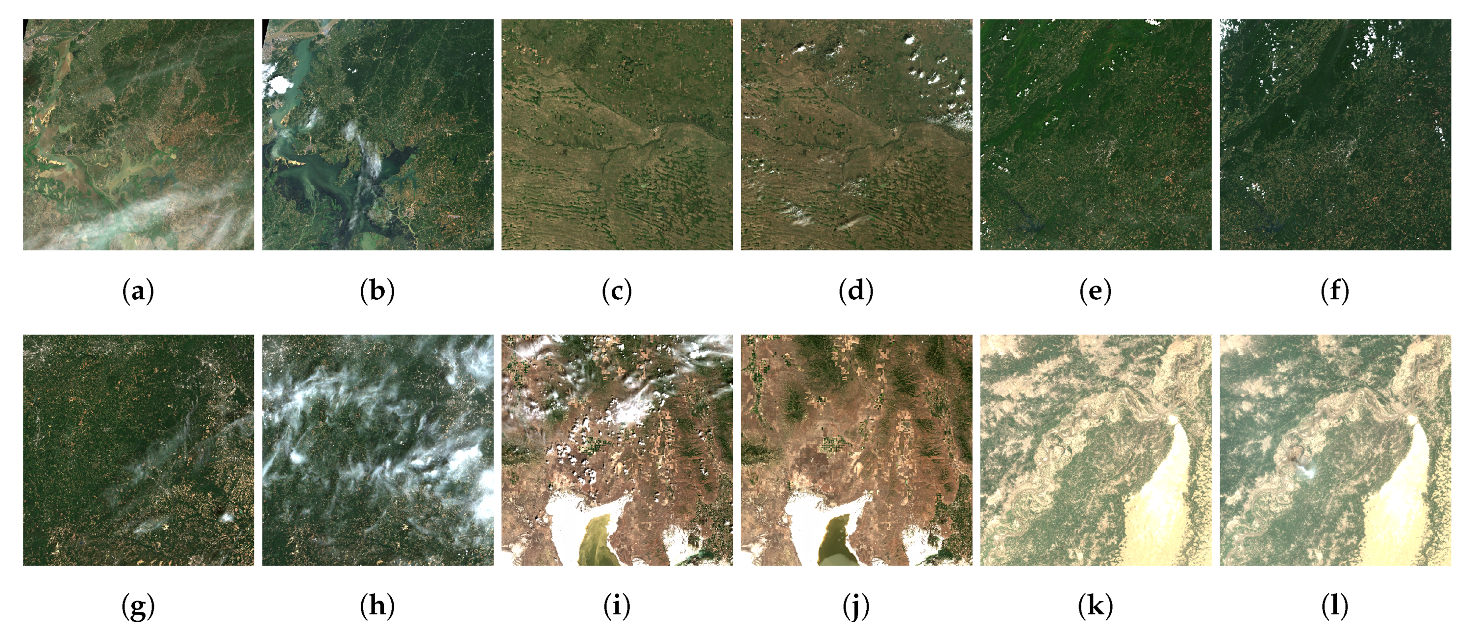
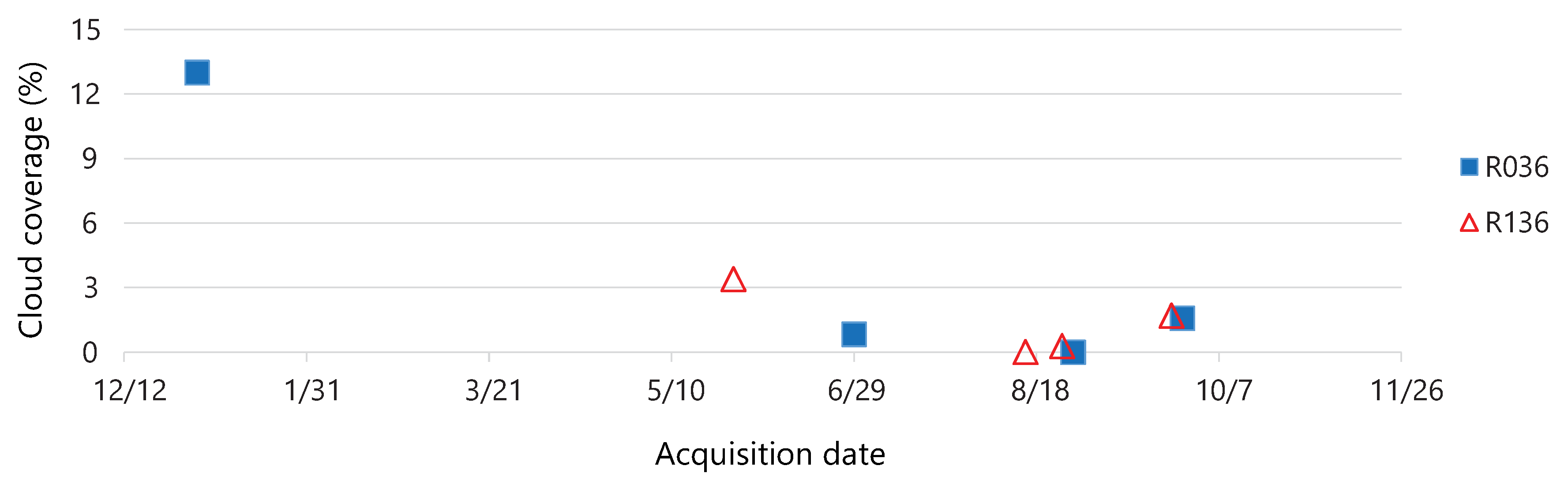
3.2. Crop Thematic Mapping Dataset

The second group of experiments relies on time series of multispectral images corresponding to the specific ground test site (area) where additional field level data were collected. Selected satellite images were used as the source of reflectance data for the design of pixel-based crop classification models, which are mutually compared and benchmarked against different lossy compression scenarios, utilizing the proposed HEVC and the chosen baseline JPEG 2000 solutions. As the result, constructed classification models differ only in the type of the training data that were used for their estimation. Thus, they differ in the degree to which different compression types influence the performance sensitivity of the chosen type of classification model (random forest), which belongs to the widely accepted and utilized family of learning machines that are present in many contemporary pixel-based thematic mapping systems.

Due to the varying cloud cover and limited vegetation season, only a relatively small subset of all available images for the chosen test site was utilized. In total, two different time series of Sentinel-2A images were chosen, corresponding to two adjacent and spatially overlapping relative orbits R036 and R136, respectively. Two orbits cover the main agricultural region in the Republic of Serbia, known as Vojvodina. Acquisition dates and the percent of cloud coverage for the two described Sentinel-2A multispectral time series are shown in Figure 3.

Orbits from Figure 3 have some spatial overlapping, as illustrated in Figure 4, however they were used separately and independently in all experiments. This was done, since the field level data were distributed uniformly over the whole region of interest, but also since images corresponding to one relative orbit have significant percent of no-data region pixels, and therefore were expected to achieve higher compression ratios in comparison to images from the other one. Also, having two classification experiments with almost the same ground-truth data, but different image sources, enables one to additionally assess stability of the obtained results and their significance.

As the result, two distinct classification datasets were designed and prepared by labeling individual pixels from the images in multispectral time series, i.e., by using ground-truth crop type labels extracted from the corresponding shapefiles that were labeled at the level of individual agricultural plots/parcels.

Characteristics of utilized Level-2 image products were already described in Section 3.1. However, it should be mentioned that the second type of experiments does not include Landsat-8 images, due to relatively small size of agricultural parcels in Vojvodina, which in the case of Landsat-8 can be only a few pixels wide, see [11]. Therefore, in order to eliminate possible influence of the spectral mixing effects onto performed compression sensitivity analysis, we have decided to exclude Landsat-8 from thematic mapping experiments, since there was no possibility to only exclude pixels laying in the crop field boundaries, due to the highly narrow shape of agricultural plots and the general lack of pixels within the fields in the case of Landsat-8.

Field level data consist of manually labeled plots corresponding to five predefined crop types (wheat, maize, sugar beet, sunflower, soybean) and an additional class corresponding to other land cover types. Each of the labeled plots was planted with only one crop type, and there was no double cropping. Labels were assigned to individual pixels inside the parcel, and their distribution per each of the categories, as well as distribution of number of corresponding agricultural parcels per each of the categories, are shown in the lower part of

Table 2. Number of agricultural fields per each of the categories in 10-fold cross-validation of mapping experiments. Partition subsets, denoted by Nº, consist of manually labeled crop fields from two different relative orbits in Figure 4, R036 and R136. Abbreviations: Ma-Maize, Wh-Wheat, So-Soybean, Sb-Sugar beet, Sn-Sunflower, Ot-Other.

Nº	Ma	Wh	So	Sb	Sn	Ot	$\mathsf{\Sigma }$	Nº	Ma	Wh	So	Sb	Sn	Ot	$\mathsf{\Sigma }$
1	26	28	14	4	11	8	91	1	23	25	11	2	11	8	80
2	26	28	14	4	11	8	91	2	23	25	11	2	11	8	80
3	26	28	14	4	11	8	91	3	23	25	11	2	10	8	79
4	26	27	14	4	11	8	90	4	23	25	11	2	10	8	79
5	26	27	14	4	11	8	90	5	23	25	11	2	10	8	79
6	26	27	14	4	10	8	89	6	22	25	11	2	10	8	78
7	26	27	14	4	10	8	89	7	22	25	11	2	10	8	78
8	26	27	14	3	10	8	88	8	22	24	11	1	10	7	75
9	26	27	14	3	10	8	88	9	22	24	11	1	10	7	75
10	25	27	14	3	10	8	87	10	22	24	11	1	10	7	75
R036	259	273	140	37	105	80	894	R136	225	247	110	17	102	77	778

and

Table 3. Number of labeled pixels in ${10}^3$ per each of the categories of random partition in Table 2.

Nº	Ma	Wh	So	Sb	Sn	Ot	$\mathsf{\Sigma }$	Nº	Ma	Wh	So	Sb	Sn	Ot	$\mathsf{\Sigma }$
1	9.5	16.8	19.0	5.3	3.5	1.7	55.9	1	21.0	9.2	3.6	1.8	10.1	1.6	47.2
2	22.3	13.5	4.2	3.3	9.0	4.0	56.1	2	5.2	26.2	4.1	6.2	2.2	2.0	46.1
3	21.1	14.5	10.7	5.4	2.0	2.5	56.1	3	22.3	6.4	2.9	1.0	7.3	6.5	46.5
4	24.4	7.8	4.4	2.4	10.0	6.1	55.2	4	14.7	17.5	5.2	0.4	2.5	6.4	46.8
5	9.5	20.5	4.1	13.8	2.9	4.1	55.0	5	5.2	11.4	9.9	3.5	7.7	8.9	46.6
6	12.3	23.5	3.1	5.6	3.9	7.3	55.7	6	14.9	17.6	5.1	2.3	2.4	4.0	46.3
7	9.5	26.1	4.4	5.0	2.6	8.0	55.6	7	7.7	16.0	14.4	0.8	2.7	4.3	45.9
8	15.1	15.7	7.0	7.3	9.1	2.4	56.7	8	25.9	9.4	4.3	0.4	3.7	2.3	46.0
9	12.6	25.4	10.8	1.2	2.5	2.5	55.1	9	11.8	9.5	9.4	3.5	5.7	7.0	46.9
10	15.4	19.5	9.3	3.0	1.9	7.1	56.3	10	10.0	24.8	6.5	0.6	2.4	2.4	46.8
R036	151.9	183.5	76.8	52.4	47.3	45.8	557.9	R136	138.7	147.9	65.3	20.9	46.9	45.5	465.1

. For example, note the table entries in the rows denoted by the symbols “R036” and “R136”, corresponding to the total number of the parcels falling into paths of the two distinct orbits of interest, respectively.

Final benchmark dataset of the labeled pixels, corresponding to the multispectral time series R036 and R136, which was utilized in all classification (thematic mapping) experiments, was obtained by random partitioning of original labeled dataset into ten disjunctive subsets. Partitioning was performed at the plot level in order to avoid that some pixels from the same field enter into another partition subset. Consequently, distribution of pixels corresponding to different crop types is not completely uniform over the 10 different, randomly generated subsets of the partition, Table 3. However, distribution of number of plots that are corresponding to different crop types over the 10 different subsets of the partition is approximately uniform, as illustrated by the entries in different rows of the Table 2.

The same subsets of the random partition shown in Table 3 were used in all performed experiments for training and testing of classification models, and the average results obtained by the corresponding 10-fold cross-validation performance evaluation procedure were reported in all cases.

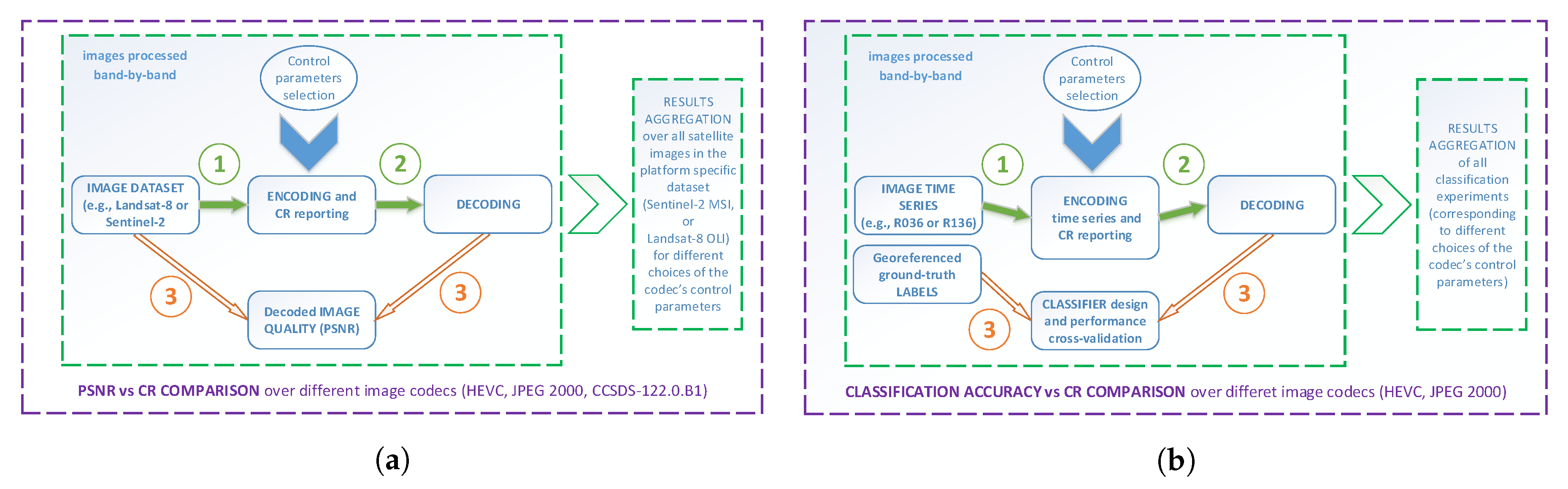
4. Experimental Setup and Methods

As previously stated, experiments are divided into two groups, or experimental setups, illustrated in Figure 5. In the following we give a detailed descriptions of all steps and explore the motivations for conducted numerical analyses presented in Section 5.

4.1. First Set of Experiments—General Coding Performance Comparison

This experimental setup was designed in order to perform the general rate-distortion performance comparison of the HEVC’s still-image intra-band coding, relative to the standard band-per-band JPEG 2000 lossy compression. Objective compression performance is measured by the means of Peak Signal-to-Noise Ratio (PSNR) vs. compression ratio curves. PSNR formulation is given with $10lo{g}_{10}\frac{L^2}{MSE}$, $MSE$ is mean squared error, and L represents the dynamic range of pixel intensities, e.g., $2^{16}-1$ for 16 b/p input data. Besides aiming at the objective assessment of lossy compression effect, we have also analyzed compression artefacts introduced by different coding approaches. A performance analysis utilizes multispectral satellite image dataset described in Section 3.1.

In the case of JPEG 2000, as the baseline lossy compression solution, a reference JPEG 2000 implementation made by [79], version 2.3.0, was used with default set of encoder parameters. Such setup includes Reversible Color Transformation (RCT) and 5/3 wavelet filter, and number of wavelet resolutions (discrete wavelet transform (DWT) decomposition level) is set to 6. Wavelet transform is applied to the whole image, thus single tile/segment is used, and the resulting wavelet transform coefficients are grouped into code-blocks (rectangular regions in the sub-band wavelet domain) of size 64 × 64. In addition, quality control parameter Q, which corresponds to the desired PSNR level, is set to some of the discrete values in the range between $[30,136]$ [dB], with the step size of 2 [dB] in-between different experiments. This gives 54 unique lossy compression quality levels obtained by JPEG 2000 per each multispectral image, per each of image bands. It is important to note that the input quality parameter is targeted value, however exact reconstruction quality level should be precisely calculated after image reconstruction by performing decoding process, e.g., see Figure 5a.

For comparison purpose only, in our general coding performance experiments we also included CCSDS-122.0.B1 image compression standard (we use CCSDS to refer to the given standard). It is based on similar coding scheme as JPEG 2000 (both are wavelet-based codecs), however with several features specifically adopted to reduce its complexity [28]. Implementation of the standard, used in our experiments, is Bit Plane Encoder (BPE) [80]. In contrast to JPEG 2000 wavelet transform, CCSDS uses integer 9/7 wavelet filter with maximum number of decomposition levels set to 3 (as defined by standard). As a quality regulation parameter, compression ratio in terms of b/p is used. In total, 55 different quality levels were obtained during experiments. CCSDS has been used in frame-based setup (with only one transform segment consisting of all image blocks), which is the most similar to computation of DWT in JPEG 2000. However, coding blocks in CCSDS are limited to 8 × 8 pixels. We have also performed some experiments in strip-based mode (with transform segments in form of strips or lines consisting of image blocks collected in raster order). However, those results were noticeably lower in terms of achieved PSNR vs. compression ratio performance.

The implementation of the HEVC’s encoder and decoder according to the standardized bit-stream is represented by the HM-15.0+RExt-8.1 reference software [69]. The set of tools is restricted to intra coding only by using encoder_intra_main_rext.cfg configuration setup, a.k.a. all intra (AI), which is the preferred configuration of the HM codec for still images. In our experiments, we use default coding settings with the respect of the given intra configuration and HM reference software. Tiles are not used in HM experiments. Essentially, the standardized version of HEVC [3] accepts input data up to 16 b/p, which makes it suitable for the applications that use high-dimensional and high bit-depth satellite data. Thus, it is also very important not to downsample satellite images prior to compression since some sensitive visual information can be lost, and this is the main reason why we have to use the range extension (RExt) version of HEVC [75]. Therefore, code is build with RExt_HIGH_BIT_DEPTH_SUPPORT and with ExtendedPrecision flag set to 1, in order to accommodate 16 b/p extension as suggested in [81]. Quality control has been given by the means of the input quantization parameter $Q_p$, where we vary its value in the range of [−48, 51] with step size of 2 in-between experiments. Note that RExt version of HEVC extends $Q_p$ for high bit-depth inputs to negative values by performing additional internal offset calculations before mapping $Q_p$ to actual quantization step size. Thus, we obtain 50 different quality levels in our experiments, which resulted in variety of compression ratios, from near lossless to high compression ratios. Although, within HEVC standardization process, common test conditions for HEVC range extensions [81] have been specified in order to have unified experimental setup used by multiple groups, we have not complied strictly with this process, especially as we turn to the specific application which is not covered under the given specification. In addition, it only defines two tiers of quality estimates (each tier uses only 4 $Q_p$ values taken in-between −37 and −16), which in our use-case is not enough to cover wider range of compression ratios and to precisely obtain application’s sensitivity to the introduced compression distortion.

Also, used default configuration of the reference codecs resulted in the best coding performance for both JPEG 2000, CCSDS, and HEVC. It should be mentioned that JPEG 2000 and CCSDS in all settings were used without an additional spectral decorrelation step before actual band-by-band image compression, which also holds for the proposed HEVC. Although there are many examples of custom encoders from the literature that suggest such spectral decorrelation step, it is usually in the context of hyperspectral images. In such case, there is much more redundancy present in the spectral domain than in the case of multispectral images. Also, since baseline JPEG 2000 performs only spatial decorrelation, HEVC analyses were focused only on the still-image coding and no spectral decorrelation was considered, e.g., utilization of inter coding mode. That part of the codec is left for our future research.

Therefore, in our setup we use per-band coding, meaning that each band is compressed individually as a separate file. Considering HEVC as video based codec, we could also re-arrange all bands of an image, resembling standard video sequence, and thereafter code all bands jointly as a sequence of bands resulting in one compressed file (although still by using intra mode only to code all bands). However, we observed that overhead information introduced by band-by-band compression is negligible when compared to the sequence coding, and almost identical performance has been obtained. Thus we chose to code bands individually to be consistent with current EO systems which are organized in a manner to perform per-band distribution. Similarly can be said for the video based Motion-JPEG 2000 (MJP2) [82], where MJP2 only defines file format for sequences of JPEG 2000 images, and where each image is coded as an independent JPEG 2000 codestream. Thus, results are obtained on per-band basis, and aggregated over image.

Regarding the PSNR vs. compression ratio performance diagrams that will be presented in Section 5.1, it should be emphasized that the presented PSNR values are averages, computed over all satellite images in Table 1. However, averaging in the case of the Landsat-8 and the Sentinel-2A/B images is slightly different, due to the fact that analyzed Sentinel-2A/B image products have varying number of image channels per each of the supported spatial resolutions of 10, 20, and 60 m (4, 9, and 11 channels, respectively). Thus, in the case of Sentinele-2A/B, in order to have a more representative average, PSNRs of individual channels where first averaged over the same spatial resolution, and then three distinct PSNR values were aggregated in the final PSNR of the same image.

Since in the most of the currently operational ground based image distribution systems user specified image orders are usually provided in the form of bulk downloads, in Section 5 compression ratio (CR) is computed over all lossy compressed images, without averaging. Such CR values correspond exactly to the possible use case scenario, like the one considered in this paper, where due to the specific characteristics of the crop thematic mapping, time series were required to be downloaded as a whole for the purpose of developing analyzed classifier instances.

4.2. Second Set of Experiments—Crop Thematic Mapping

The other set of experiments is oriented towards the analysis of the compression induced distortion effects on the specific thematic mapping application. Experiments are conducted on the proposed Sentinel-2A benchmark dataset given in Section 3.2. Since presented analysis also aims to offer application oriented comparison of HEVC’s performance, as the foundation for the second set of experiments, a classic problem of pixel-based crop classification in multispectral satellite images using time series of georeferrenced surface reflectance measurements has been chosen. Such data capture the time varying phenology of the plants and make required category discrimination much more effective. In order to simplify the experimental setup, and enable a fair comparison in terms of sensitivity of classification performance to various effects caused by different lossy compression scenarios, instead of object-based classification approach we have decided to rely on pixel-based classifier. As opposed to object-based approach, it performs feature space partitioning by using measurements aggregated only at the level of individual pixel, which eliminates possible improvements that could arise from incorporation of pixel’s neighbourhood, or enhancements resulting from the postprocessing of pixel-based decisions at the object level. However, such pixel-based approach is widely accepted solution, which is used in many operational thematic mapping systems.

Thus, classification performance, which is intended to be used as an indicator of the thematic mapping’s sensitivity to compression effects, is influenced only by the quality of measurements at the level of individual pixels, and not by the spatial resolution of the sensor nor the structure of pixel’s neighbourhood. However, through comparison of classifier’s performance with the same type of decision system utilizing original, uncompressed data, such pixel-based classifier is still capable of highlighting and reflecting the level of preserved quality of original measurements after compression, relative to the uncompressed baseline. Potentially, this could be very important in some other applications besides thematic mapping, which could be oriented more towards computation of plants’ biophysical parameters, or that would rely on multispectral satellite images with coarser spatial resolution than Sentinel-2. On the other hand, experimentally measured performance of such pixel-based classification approach does not reflect the effects of compression on simple image primitives like edges and textures, which could be important in the case of higher resolution sensors and predefined or learned object-based image descriptors. However, such effects are possible to estimate in other ways, including visual inspection of higher resolution lossy compressed images and their comparison with their coarser resolution counterparts, like Landsat-8 images of the same scene. Therefore, this was particularly considered in the set of the conducted experiments of the first type, described in Section 4.1‚ where the compression performance was analyzed from the general, and not an application oriented perspective.

As the type of an adequate classification model for the specified thematic mapping task was used random forest [83], which possesses high generalization capability due to its intrinsic ensemble structure and the fact that decision trees [84] are particularly suitable for partitioning of feature space based on simple, yet very informative features corresponding to time varying spectral signatures of the Earth’s surface.

In order to remove any classification performance bias coming from the specific classifier design or feature extraction pipeline, in all conducted experiments was used the same classification setting as proposed in [11]. It consists of feature level fusion that extracts surface reflectance measurements corresponding to the same image pixel from all bands of all images in the corresponding time series. This step is followed by an ensemble type random forest classifier with 100 trees of variable depth (adaptive splitting until all leaves are pure or contain only two samples), and splitting criterion based on the Gini index and sampling of $\sqrt{d}$ random features in each node, where d is the total dimensionality of the feature space. Classification was implemented in the Python programming language, using library [85].

However, since individual bands of Sentinel-2 images have varying spatial resolutions (see Section 3.2), before final feature extraction all multispectral images were: (1) compressed at their nominal spatial resolution (except in the case of classification model based on uncompressed image data), and afterwards (2) in the case of 20 m and 60 m Sentinel-2 image channels additionally upsampled to spatial resolution of 10 m using nearest neighbour interpolation method. The second step is necessary since we are interested in exploiting as much of available spatial information during the decision process, e.g., fine signal variations present in 10 m image channels are valuable in the presence of small crop fields. We would also like to add that the practical implementation of this step does not require allocation of new memory, since 20 m and 60 m image pixels are just indexed several times during the feature extraction process, in accordance with their spatial position in the physical coordinate system. Thus, classifier decisions were made at the highest level of detail, i.e., at the level of pixels with 10 m of spatial resolution.

Each of the experiments that are introduced in this subsection correspond to the performance analysis of the selected random forest classifier that was trained and tested using the labeled benchmark dataset described in Section 3.2, which was initially randomly partitioned into 10 subsets in order to enable classifier performance evaluation based on 10-fold cross-validation procedure. It should be noted that each of the experiments is utilizing different type of source data, i.e., the same Sentinel-2A multispectral images (time series), but with different type and level of lossy compression. Thus, the performance of the baseline classification model is evaluated using uncompressed image data, while the rest of experiments are conducted using lossy compressed image time series, obtained with different sets of encoding control parameters in each experiment, i.e., by varying HEVC and JPEG 2000 configurations. These configurations were varied in the same manner as in the case of the first set of general compression experiments that were described in Section 4.1. The only difference is that instead of both Landsat-8 and Sentinel-2A/B data, in classification experiments only Sentinel-2A data were utilized.

Since for the selected area we have collected two separate image time series, denoted as R036 and R136, each of the above mentioned experiments was conducted twice, once for each of the two Sentinel-2A relative orbits. Alternative option would be to combine all these measurements together. However, as already mentioned before, using data from R036 and R136 separately gives possibility to mutually compare results of two individual classification analyses under similar experimental setting. Also, combining data from R036 and R136 would slightly reduce the overall number of training and test samples per each class in the benchmark dataset. Therefore, such alternative dataset design strategy was avoided.

5. Results Analysis and Discussion

All results are presented according to the plan of experiments developed and presented in Section 4 with level of presentation details adapted to the large number of numerical simulations.

5.1. General Compression Performance Comparison

From the perspective of the general compression performance, results from the first set of experiments, Figure 5a, confirm initial hypothesis that HEVC still-image intra band coding can be considered as an adequate standardized solution for effective lossy compression of multispectral satellite images.

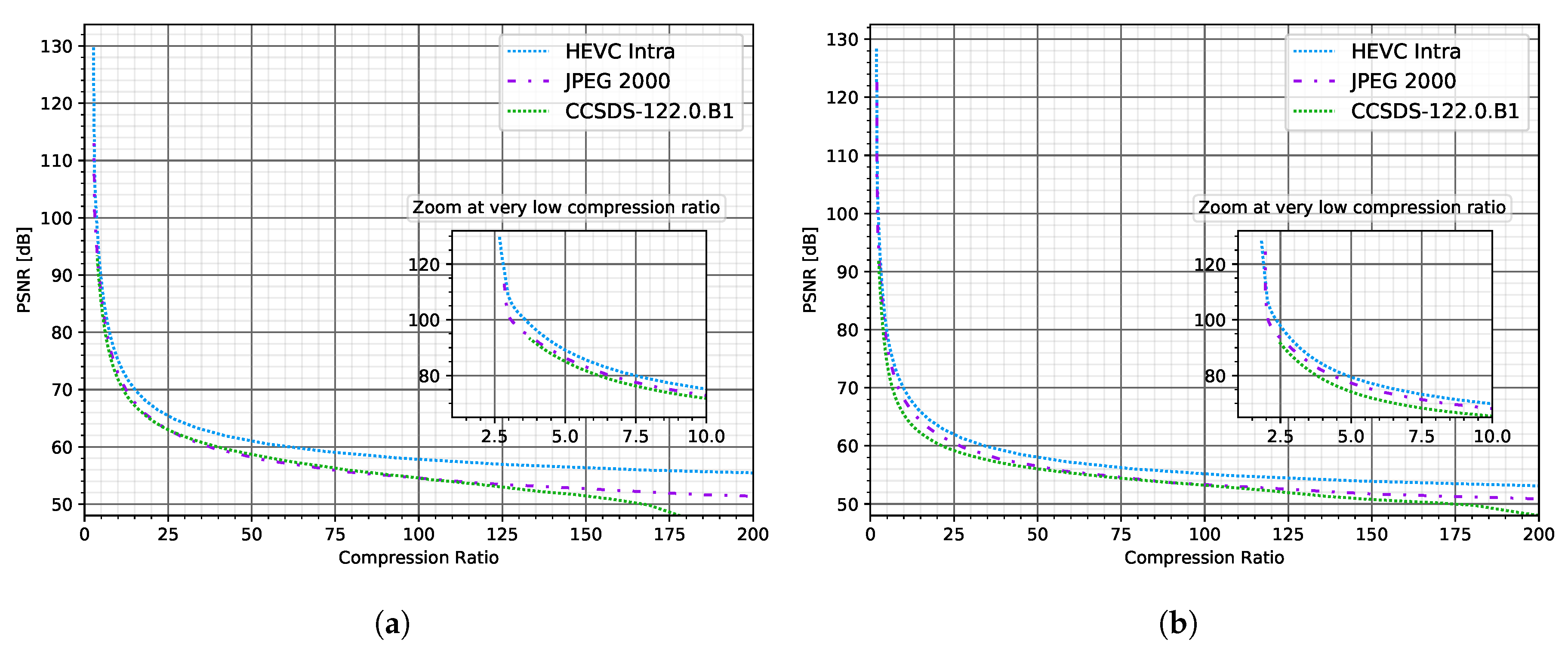
5.1.1. PSNR vs. CR—Results

Figure 6 and

Table 4. Achieved compression ratios (CR) at the same level of PSNR. Performance of HEVC is expressed relative to JPEG 2000 and CCSDS 122.0.B1 CRs over two parts of the proposed dataset.

	Landsat-8 CRs
PSNR	HEVC	JPEG 2000	Rel. Diff. [%]	CCSDS	Rel. Diff. [%]
55	229.84	89.04	158.13	93.19	146.63
60	60.66	37.14	63.33	39.78	52.48
65	26.29	19.68	33.59	19.30	36.22
70	15.04	12.36	21.68	11.56	30.10
	Sentinel-2A/B CRs
PSNR	HEVC	JPEG 2000	Rel. Diff. [%]	CCSDS	Rel. Diff. [%]
55	103.94	66.17	57.08	65.02	59.85
60	34.11	26.69	27.80	21.46	58.94
65	16.57	13.69	21.04	10.48	58.11
70	9.84	8.34	17.99	6.56	50.00

neatly summarize the codecs general performance over the two proposed image datasets corresponding to—Landsat-8 and Sentinel-2A/B, which were described in detail in Figure 2 and Table 1. Presented results also highlight variations in compression performance due to differences in the type of studied image sensors.

5.1.2. PSNR vs. CR—Analysis and Discussion

Regarding the performance comparison between JPEG 2000 and CCSDS image coding standards, from Figure 6, we can observe that CCSDS codec perform on par with JPEG 2000 over the majority of the CRs. The CCSDS results were close, or sometimes even lower, to the results obtained by the JPEG 2000. Therefore, this codec was left out from the further discussion, e.g., classification sensitivity analysis. In addition, at higher CRs we note significant deterioration in performance for CCSDS codec. However, it is expected since CCSDS was not designed to operate on such high CRs.

As measured by preserved image quality, HEVC has shown greater resilience to information loss, i.e., ability to achieve higher CRs at approximately the same image quality levels as compared to JPEG 2000. Thus, it can be seen that Landsat-8 images, Figure 6a, tend to be compressed more efficiently, e.g., have higher compression ratios for the same level of PSNR, when compared to their Sentinel-2 counterparts, Figure 6b. Therefore, relative difference between HEVC and JPEG 2000 performance is higher when benchmarked exclusively over Landsat-8 part of the adopted general purpose dataset, which is also summarized in Table 4. This could be explained by the presence of no-data regions, which are always found in Landsat-8 images (dark/blank areas in the corners of the scene, present due to orientation of satellite orbits with respect to the image reference system). In contrast, this is not always the case for Sentinel-2 images (especially in the proposed Sentinel-2A/B part of our general performance comparison dataset, which turns out to have a very low proportion of no-data regions). Such blank, uniform regions are naturally easier to be compressed by using block based approach (characteristic for HEVC), as opposed to wavelet decomposition that is performed on an image as a whole (in the selected baseline JPEG 2000).

We also remark that HEVC brings substantial savings in the required rate in comparison to JPEG 2000, as it can be seen from Figure 6 and Table 4. In particular, for mid compression ratios (high PSNR range, between 65 [dB] and 70 [dB]), HEVC brings from 17.99% up to 33.59% savings in the required rate with respect to JPEG 2000 (as measured by the relative difference in achieved compression ratios over Sentinel-2A/B and Landsat-8 parts of the proposed benchmark dataset, respectively, Table 4). Furthermore, HEVC achieves up to 63.33% reduction in rate over JPEG 2000, for high compression ratios (low PSNRs) represented by the 60 [dB] entry in Table 4 corresponding to the results obtained over Landsat-8 part of the proposed dataset. As it can be seen from Figure 6 and Table 4, savings are even higher at 55 [dB], but this range of image quality is already below the one desirable for crop thematic mapping applications (see Section 5.2). Thus, for very high compression ratios HEVC can achieve even up to 158.13% of rate improvement over JPEG 2000, as measured over Landsat-8 images, which is lower for Sentinel-2 images and goes to 57.08%, due to already mentioned lower presence of no-data regions that are characteristic for Landsat-8 images.

Additionally, in Figure 6 we can see that the performance on very low compression ratios (around 2–3) does not show significant difference between the two benchmarked codecs. Moreover, JPEG 2000 was able to slightly outperform HEVC, as shown in the zoomed part of the diagrams in Figure 6. However, performance for very low compression ratios should be additionally investigated in greater detail, e.g., by benchmarking obtained lossy compression results with the lossless versions of the same codecs, which should be considered as a more appropriate design choice for the described, specific operational range. Our assumption is that the same compression ratios could be achieved by lossless modes, leading to a perfect reconstruction. Also, lossless modes usually posses less computational complexity. However, such analysis is left out from this study and could be part of potential future work.

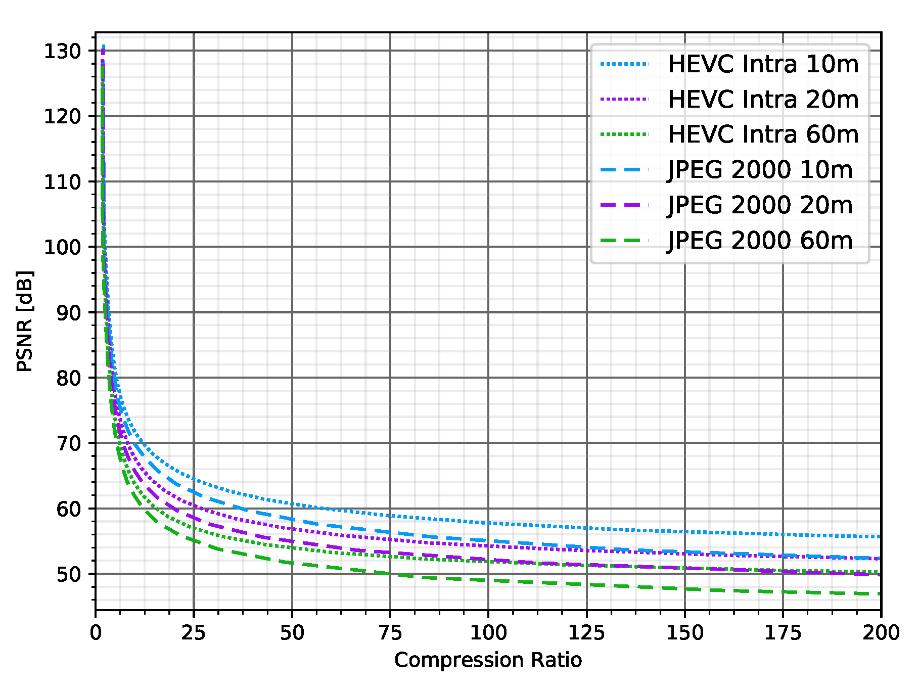
5.1.3. Resolution Effects—Results

Since Sentinel-2 image products contain image channels with varying spatial resolutions, this specific property was exploited to additionally investigate effects of the pixel size on the compression performance. These results are summarized in Figure 7, where for each spatial resolution of 10, 20, and 60 m, computed average PSNRs are depicted against the achieved compression ratios.

5.1.4. Resolution Effects—Analysis and Discussion

We can see that both codecs perform better on higher resolutions (blue lines). Moreover, HEVC (represented by dotted lines) always shows higher performance margin in comparison to JPEG 2000 (dashed lines), at all spatial resolutions (which was already expected based on the results presented in Figure 6). However, HEVC’s advantage is particularly exaggerated at the highest level of details, corresponding to 10 m spatial resolution, where, e.g., at 60 [dB] we can see significantly higher margin between HEVC and JPEG 2000’s compression ratios, as compared to other spatial resolutions. This was natural to expect, since images with higher spatial resolution have higher presence of uniform image regions, and these regions are also expected to have larger size (image extent in pixels) in comparison to images with coarser spatial resolution of 20 m, or 60 m per pixel.

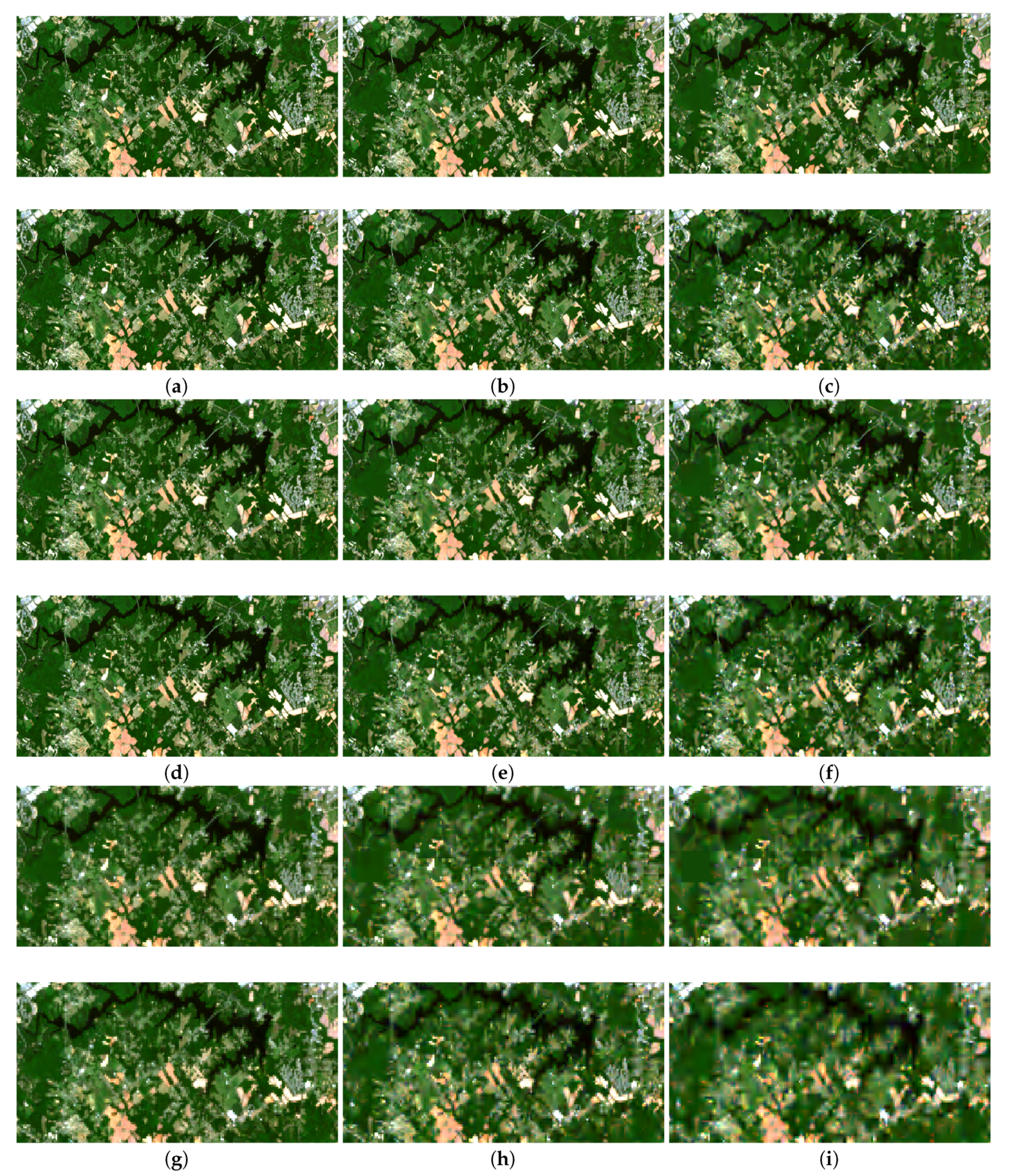
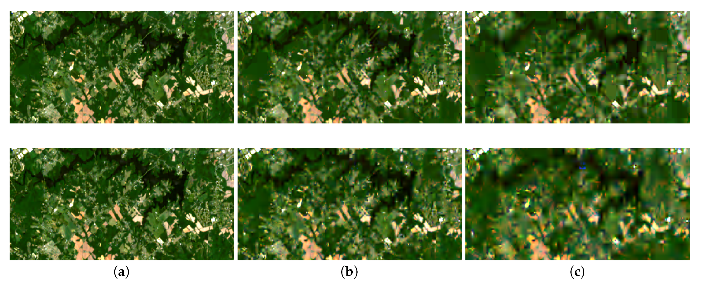
5.1.5. Visual Comparison—Results

As an adequate testbed for qualitative assessment of the benchmarked codecs we have selected an image region with the complex scene content, corresponding to agricultural holdings, forest and water bodies in North Carolina, entry Nº 7 form Table 1. Visual illustrations of the obtained results are presented in Figure 8, where true color composites of original images are ordered according to Sentinel-2 image spatial resolutions (10, 20, and 60 m) and the selected, representative levels of PSNR (56, 60 and 70 [dB]). True color composites of lossy compressed 30 m Landsat-8 image of the same region are also presented in Figure 9.

5.1.6. Visual Comparison—Analysis and Discussion

As expected, visual inspection of results in Figure 8 and Figure 9 reveals that in the case of both codecs the presence of compression artefacts is becoming more significant after the mid-range of 60 [dB] (the last two columns). Also, compression effects are dependant on spatial resolution, and the perceived rate of image degradation is higher towards the lower resolutions of 20, and 60 m, even at the same level of PSNR (e.g., Figure 8e,h or Figure 8f,i).

However, it is particularly interesting to note that, based on visual comparison, HEVC outperforms JPEG 2000 even at the same level of PSNR, consistently over all spatial resolutions. This is easiest to see at 60 [dB], even at the highest spatial resolution of 10 m, Figure 8b. In addition, savings introduced by the HEVC’s higher compression ratio over JPEG 2000 at the same PSNR level of 60 [dB], were already shown to be 27.80%, Table 4. Thus, besides the significant gain in achieved compression ratios in the case of the proposed HEVC solution, visual inspection confirms that the object boundaries are also better preserved, i.e., object boundaries in the image are much sharper and have a more precise shape with less visual distortions (blurring effect). For example, lake and field boundaries in the upper part of Figure 8b, and objects at smaller spatial scale. For the best comparison, 10 m images in Figure 8b should be analyzed enlarged, side by side, at the computer screen.

Differences in compression effects among HEVC and JPEG 2000 at high PSNR of 70 [dB] are definitely more subtle (the first column in Figure 8). However, based on objective assessment there is still significant relative difference in achieved compression ratios between HEVC and JPEG 2000 at this high PSNR range (from 17.99% up to 21.68% according to Table 4).

Regarding comparison over 30 m Landsat-8 image, Figure 9, it is worth mentioning that by visual inspection at mid and low PSNR range it is easier to become aware of blocking artifacts introduced by HEVC, in comparison to 20 m or even 60 m Sentinel-2 images with same image quality in Figure 8 (e.g., compare Figure 8h and Figure 9b). Latter is rather strange, since 30 m image contains four times more pixels than a 60 m one. However, it can be explained by the scale of objects present in the scene and the fact that a 60 m image channel inherently already has significant amount of spectral mixing (less features of the scene geometry), i.e., only large scale scene details are recorded in the uncompressed original image.

Again, HEVC shows better ability to preserve image details (e.g., lake boundaries), however it is less obvious than in the case of 10 m and 20 m Sentinel-2 images due to lower spatial resolution (especially at lower PSNRs, the last two columns). As expected, results also reveal that at lower spatial resolutions and PSNR levels more blocking effects are present. E.g., when the upper image in Figure 9b with a 60 [dB] is enlarged next to the upper image in Figure 9a (which at 70 [dB] is very close to the 30 m uncompressed original).

5.2. Application Oriented Compression Performance Comparison

In addition to the general compression performance analysis, it is also tempting to validate previously presented results from the standpoint of some practical remote sensing application. Thus, in the following are the analyses measuring sensitivity of the specific remote sensing classification task in the presence of lossy compressed input data. The same set of experiments, illustrated in Figure 5b and described in Section 4.2, was conducted twice, independently over two different subsets R036 and R136 of the prepared ground-truth dataset introduced in Section 3.2.

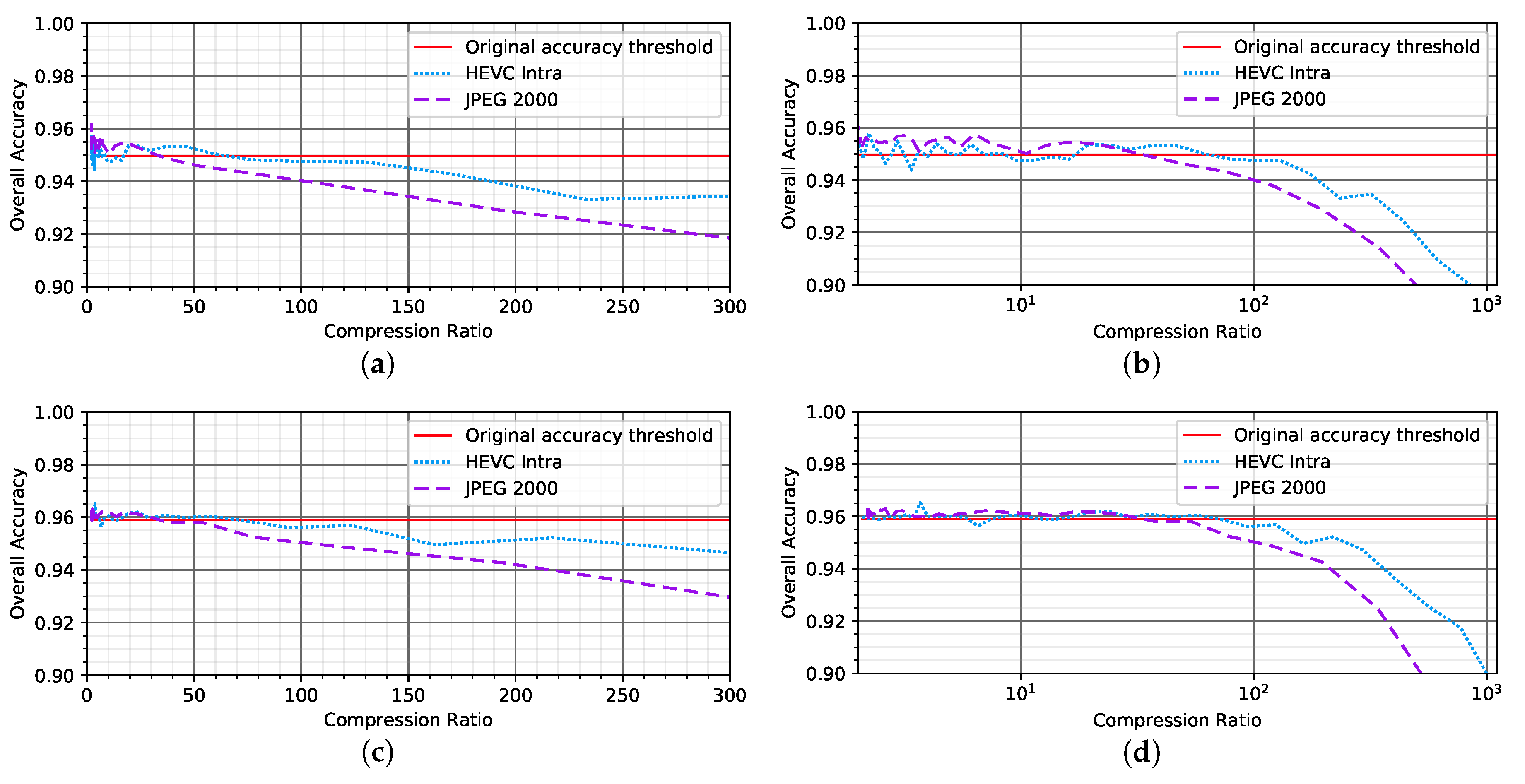
5.2.1. Classification Sensitivity—Results

Performed analyses consist of benchmarking classifiers’ performance against the lossy compressed images generated by the HEVC and the JPEG 2000. This means that for the each of the codecs’ configurations (driven by different values of the corresponding quality control parameters), datasets R036 and R136 were lossy compressed each time, and the new instance of the same learning model type was trained and tested.

Thus, in Figure 10, for each experiment (classifier instance), a pair of values corresponding to the overall classification accuracy (OA) and the achieved compression ratio (CR) was plotted. For the sake of completeness, in

Table 5. Accuracy assessment matrices for two classifier instances based on the original, uncompressed time series data, R036 and R136. Symbols are the same as in Table 2. Values represent number of pixels in ${10}^3$. Column labels denote classifier decisions, while the row labels represent true crop categories. Overall accuracy (OA), Cohen’s Kappa statistic (KP) and the KP confidence intervals (CI) are given at the bottom of the table.

R036	Ma	Wh	So	Sb	Sn	Ot	R136	Ma	Wh	So	Sb	Sn	Ot
Ma	148.6	0.4	1.5	0.2	0.9	0.1	Ma	137.0	0.3	0.5	0.0	0.6	0.1
Wh	0.5	181.6	0.6	0.0	0.3	0.4	Wh	0.3	146.7	0.0	0.0	0.2	0.7
So	4.7	0.3	67.0	1.4	3.2	0.2	So	0.9	1.4	60.6	0.1	2.0	0.3
Sb	0.6	0.1	0.5	51.0	0.2	0.0	Sb	0.0	0.0	0.2	20.5	0.1	0.0
Sn	1.3	0.4	0.4	0.3	44.7	0.1	Sn	1.0	0.5	0.1	0.2	45.0	0.1
Ot	4.9	3.1	0.3	0.1	0.8	36.6	Ot	0.5	8.4	0.2	0.1	0.0	36.2
$\mathrm{OA}=94.95$%  $\mathrm{KP}=0.94$  $\mathrm{CI}=\left[0.93390.9354\right]$							$\mathrm{OA}=95.90$%  $\mathrm{KP}=0.95$  $\mathrm{CI}=\left[0.94710.9456\right]$

, are also provided results of the two classifier instances based on the original, uncompressed image data, while their OAs are plotted by the solid red lines in Figure 10.

5.2.2. Classification Sensitivity—Analysis and Discussion

Based on Figure 10, it can be said that the initial assumption regarding the possibility of lossy compression having a positive impact on the classification performance at low compression ratios proved to be valid, since the compression side effects (e.g., noise canceling) led to better classifier performance at lower CRs, in the case of both benchmarked codecs and for the both R036 and R136 test subsets. Also, in Figure 10 we can see that the JPEG 2000 performs quite well for the CRs of up to 35:1 (dashed lines), mostly without any loss in performance when compared to the original classifiers, which were trained and tested on the uncompressed data (red lines). At the same time, HEVC (dotted lines) can achieve the same (or even better) classification accuracy in comparison to the original classifiers (OA’s represented by the red lines), even at compression ratios of up to 70:1, leading to a nearly 100% relative improvement in achieved CR (potential savings) over JPEG 2000. The range of compression ratios leading to such OAs, which are close to the ones achieved by the original classifiers, could be regarded as the first operational range, when considered in the context of the selection of an optimal compression strategy. Therefore, points towards the end of the described range should be regarded as the effective codec configuration choices for efficient distribution of the lossy image data applied in crop thematic mapping. Moreover, since high temporal resolution signatures of the vegetation pixels require dense image time series, any potential savings in storage and communication requirements could be significant in the case of the constrained time or memory resources.

On the other hand, JPEG 2000 is able to provide sufficiently high classification accuracies when data are compressed with CRs of up to 60:1 for R036, or 70:1 for R136, maintaining OA within the acceptable loss margin of 0.5%. However, HEVC has demonstrated ability to maintain approximately the same classification performance (losing no more than 0.5% of accuracy) for CRs of up to 150:1, in the case of R036, and up to 140:1, for R136 test subset, as in Figure 10. It is a limit after which distortions begin to have significant influence on the overall classification performance. For example, in comparison to HEVC, at same CR JPEG 2000 loses on OA are around 1.5% and 1.2% for R136 and R036, respectively.

Therefore, breaking points of HEVC and JPEG 2000 curves in Figure 10 could be considered as the examples of the indicators designed to measure codec’s expected performance in application oriented lossy compression scenarios. Implications of the presented sensitivity analyses, conducted over both R036 and R136, confirm that at the relatively high CRs (which are determined by the application specific, performance loss margin) the proposed HEVC based solution is able to better preserve features important for more accurate classification, as compared to the JPEG 2000, when the same CR has been accounted for—leading to the higher savings in storage and communication requirements of the ground based data distribution segment.

Although it may not be considered to be of significant practical importance for the considered application task, codecs’ behavior for the higher compression ratios (with loss margin larger than the 0.5% of the overall accuracy of the original classifier) is also shown in Figure 10b,d.

In the context of the crop thematic mapping, spatial dependant relationships may be an important part to analyze in more detail. However, significance of the particular, individual image channels and the impact of the level of distortion introduced during compression at different spatial resolutions on the overall classification accuracy will be the subject of our future work, especially from the standpoint of adaptive control parameter selection for optimal compression performance and classifier design.

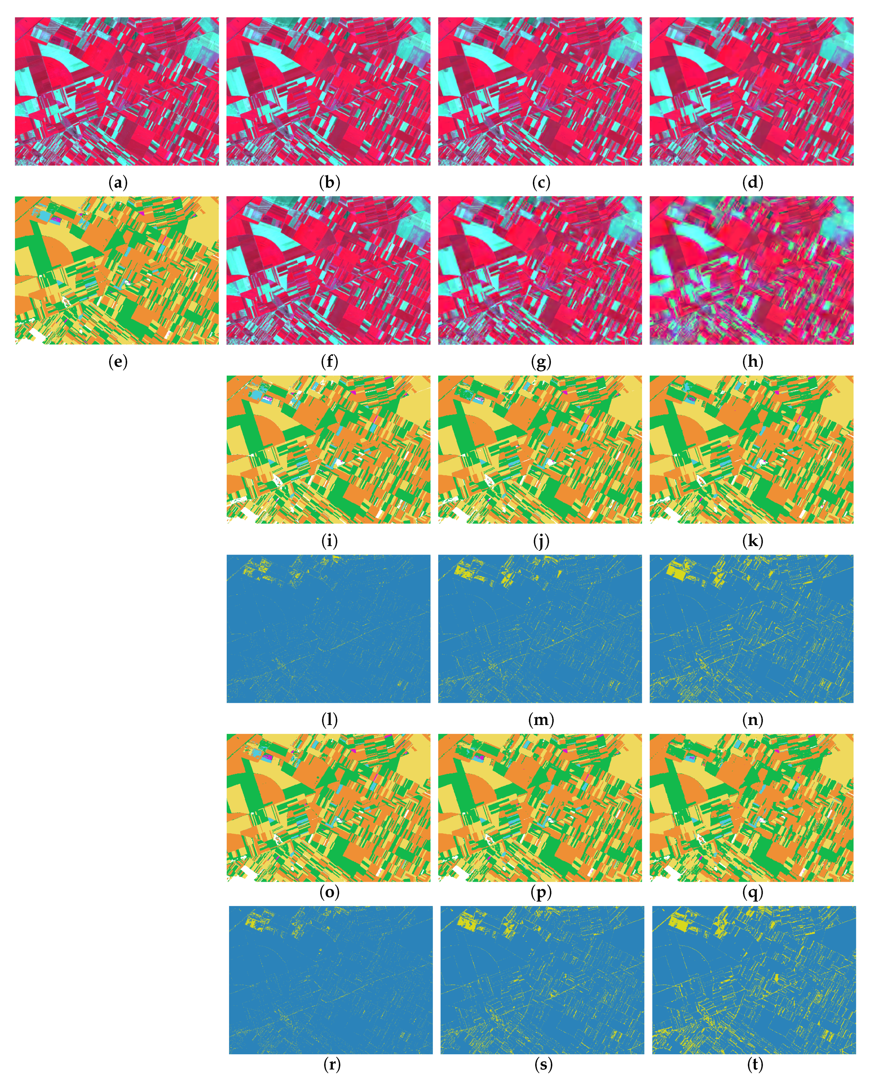
5.2.3. Crop Thematic Maps—Results

Besides the comparative quantitative analyses presented in Figure 10, in order to further discuss the performance of HEVC and JPEG 2000 based solutions, we also provide a type of qualitative assessment of the achieved classification performance. It is based on the visual inspection of the obtained crop thematic maps and their differences, see Figure 11.

As the result of HEVC’s higher effectiveness, as shown in Section 5.1, it was expected that HEVC based lossy compressed images should also generally provide better application oriented performance (higher quality crop thematic maps). In particular, it was expected that even at low CRs, where there is less difference between HEVC’s and JPEG 2000’s performance, visual inspection of the corresponding thematic maps should also reveal better visual quality of classification maps produced using HEVC encoded images. This was the main motivation for illustrations presented in Figure 11, which have confirmed described initial assumptions, and gave additional insights into complex relationship between lossy compressed image quality and classification performance.

5.2.4. Visual Comparison of Classification Maps—Analysis and Discussion

Examples in Figure 11 were selected in order to indicate an important fact - that the classification maps obtained by the HEVC and the JPEG 2000 with approximately the same CRs (around 25:1, 75:1, and 200:1) result in the crop thematic maps that are visibly more accurate in the case of the HEVC compression. This can be confirmed by the visual comparison of the corresponding difference images, computed between the map produced by original classifier and each of the maps produced by HEVC and JPEG 2000 based solutions (obtained at the same CR), i.e., by comparison of: Figure 11l vs. Figure 11r; Figure 11m vs. Figure 11s; and Figure 11n vs. Figure 11t. Difference images reveal changes in decision maps made by the original classifier (relying on uncompressed data), Figure 11e, and the maps produced by the three selected lossy compression instances of the same classification model, illustrated in Figure 11i–k,o–q.

Thus, by inspection of the given pairs of figures, it is clear that at all considered CRs (corresponding to different columns of Figure 11), there are always more yellow pixels (dissimilarities) in the case of JPEG 2000, as opposed to HEVC based solution. It is interesting to see that differences are also visible in the case of low compression ratio, e.g., 25:1, where HEVC produces visually better map, compare Figure 11l against Figure 11r, even that classifiers’ OA is approximately the same at the given CR, e.g., see Figure 10. The same trend is even more exaggerated at the higher CR’s (column 3–4), where according to the previously presented results HEVC achieves even better level of the corresponding quality-compression trade-off against JPEG 2000. However, it should also be noted that in both cases, at low CRs (second column) classification maps are the most sensitive to compression effects affecting fine image details, like the boundaries between fields or the lines corresponding to roads. This is understandable, since at the boundaries of different objects in the scene there is naturally more spectral mixing and it is harder to delineate different categories in the corresponding feature space, which makes them the most sensitive to any signal variations. On the other hand, as expected, higher CRs result in noisier maps, or even complete misclassification. Again, smaller fields, which are harder to delineate, are more suspectable to errors. In addition to the above discussion, we would also like to note that the presented map differences at lower CRs (higher PSNR) are not necessarily corresponding to classification errors, since the map in Figure 11e does not represent the ground-truth, but the decisions of the original classifier instance (which is also prone to errors), while the previously presented quantitative analyses revealed that the small amount of lossy compression can have a noise canceling effect and bring additional improvements in the overall classification performance.

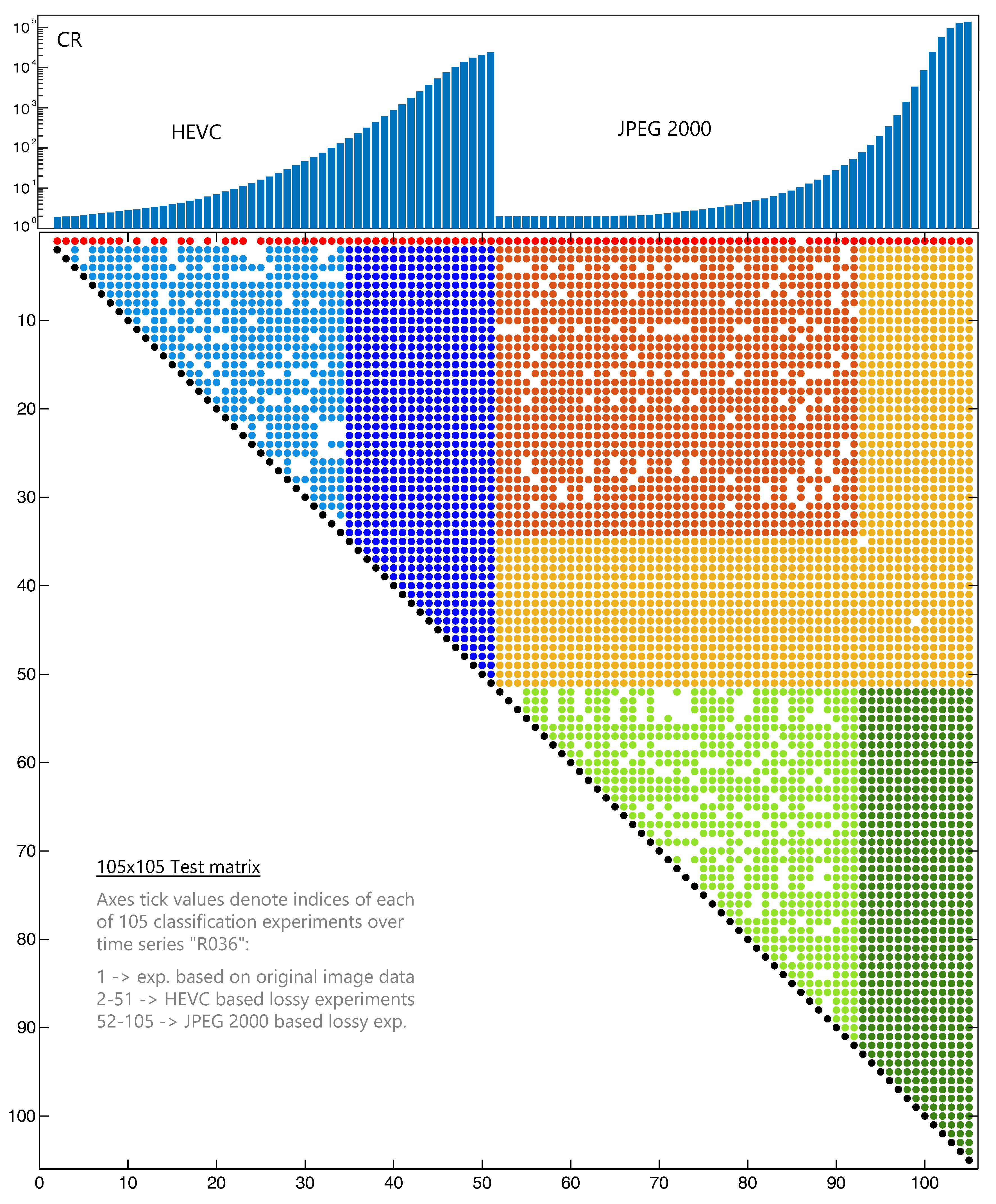
5.3. Classification Results from the Statistical Significance Perspective

Since presented sensitivity analyses in Section 5.2 were based on extensive numerical simulations, there is a question of statistical significance of difference between results corresponding to different classifier instances, i.e., lossy compression experiments driven by different values of corresponding HEVC and JPEG 2000 control parameters, Figure 5b.

In total, for each R036 and R136 dataset there were 10⁴ unique numerical experiments, 50 corresponding to HEVC and 54 to JPEG 2000, covering approximately the same range of image quality levels. Each of the reported outcomes, plotted in Figure 10, represents the statistically cross-validated classification performance measure, i.e., in the given case overall accuracy (OA). However, for the purpose of measuring statistical significance of difference between each pair of conducted experiments, we have decided to analyse another aggregate performance measure, the Cohen’s Kappa coefficient [86], which compactly integrates both “type I” and “type II” classification errors into one representative performance measure, i.e., efficiently aggregates the off-diagonal elements present in the corresponding accuracy assessment matrix of each experiment. Thus, for each pair of the experiments, represented by the estimated Kappa coefficients, the null hypothesis of two Kappa values being the same was tested with the level of 5% of statistical significance. Results of all statistical tests are graphically presented by the upper triangular matrix in Figure 12, with circles denoting the positive outcomes (rejection of null hypothesis).

Thus, when present, circles above the main diagonal denote that the experiments’ outcomes (Kappa coefficients) were significantly different, while the elements on the main diagonal (except the first one) denote that the each of the associated experiments resulted in classification that was significantly different from the one expected by chance. Finally, indices of the first element in the 10⁵ × 10⁵ test matrix in Figure 12 denote the original classifier, based on the uncompressed image data from the time series R036.

5.3.1. Analysis of Observed Patterns and Discussion of Their Implications

Figure 12 shows that in the most cases experiments based on different (lossy compressed) input data resulted in different classification performance. Presented illustration also reveals that for some choices of codecs’ configuration parameters (varied in the defined range of values by the constant step size) there appear small “clusters” of empty circles, i.e., experiments resulting in classification performance that could be regarded as the same in the statistical sense. However, the most interesting insight is that observed clusters can be visually grouped into different “compression comparison zones”, or regions, illustrated by different colours in Figure 12. Moreover, the regions seem to be not arbitrary, but aligned with the experiments corresponding to different working regimes (compression ratios) of the compared HEVC and JPEG 2000 image codecs. Therefore, besides the test matrix, upper part of Figure 12 also includes the graphical illustration of the computed CR for each experiment (the bar diagram that is aligned with the matrix columns and shown in the log scale). The bar diagram also has an additional purpose, to delineate matrix columns (i.e., rows) corresponding to experiments considering HEVC and JPEG 2000. Therefore, with the help of the bar diagram, it is easy to distinguish between the two, by considering the two distinctive parts of the diagram—the first one on the left, representing the HEVC related CRs, and the second one on the right, depicting considered JPEG 2000 configurations.

In Figure 12 we have identified several regions, which is also reflected in the choice of the selected colours. Thus, the light blue and the dark blue regions correspond to the tests of statistical significance among the experiments exclusively utilizing the HEVC based data with different CRs, while the light green and the dark green correspond to the experiments exclusively based on the JPEG 2000 input data. The remaining regions, the orange one and the “L” shaped yellow one, correspond to crosswise tests among experiments based on different configurations of the HEVC and the JPEG 2000.

Last, but not the least important, is the group of tests illustrated by the red colour, the first row of the test matrix in Figure 12. It illustrates the significance of difference among all 104 “lossy classifiers” and the “original” classifier (based on the uncompressed image data and represented by the the first element of the test matrix, i.e., by the first “missing” circle in the first row). The red region, i.e., the first row, reveals that there are more empty spaces (missing circles) among the set of columns in the first row that are representing the HEVC solution, as opposed to the one associated with the JPEG 2000. This is another confirmation that among the HEVC based classifiers operating at the relatively moderate compression ratios (up to 16:1), there are more classifiers that can achieve the classification performance that is (in the statistical sense) the same as as the one achieved by the original classifier—as compared to the JPEG 2000, which has only one empty circle in the red region of the given example in Figure 12 (at CR of 13:1). Moreover, when compared by using described Kappa based tests of statistical significance, it is also clear that the bar values (CRs) corresponding to the missing red circles in Figure 12 grow faster in the case of the HEVC, as compared to the CR entries preceding the missing red circle in the case of the the JPEG 2000. This is in full accordance with the results and implications of the previously discussed sensitivity analysis in Figure 10a, where the HEVC was able to preserve the OAs close to the original one much longer, in comparison to the JPEG 2000 (up to significantly higher CRs).

We would also like to note that in the Figure 10a the breaking points of the HEVC and the JPEG 2000 performance with respect to the OA of the original classifier (red line), were at CRs of 70:1 and 35:1, respectively, Figure 10a. In both cases, these values are significantly higher than the above mentioned Kappa based CRs with similar interpretation, in Figure 12. This indicates that establishing equivalence between lossy compression based solutions and original classifier, besides being application dependant also requires careful consideration of the adopted metrics. However, we should also emphasize that the red circles in the first row of Figure 12 do not indicate to what extent an experiment with the OA close to the one achieved by the original classifier is different (like in the case of the red circle in column 32 of the test matrix, closely corresponding to the HEVC’s CR limit of 70:1). However, in the given case, based on Figure 10a, we can say that their (OA) performance is almost the same.

In the column direction, the triangular light blue HEVC region in Figure 12 ends at CR of ≈130:1 (column 34 of the test matrix), while the light green JPEG 2000 region ends at CR of ≈53:1 (column 92). The shared characteristic of both triangular regions is that they correspond to relatively low CRs, as well as to the statistical tests performed exclusively among the pairs of experiments based on the same type of compression algorithm (HEVC or JPEG 2000).

The fact that in the light blue and the light green matrix regions there is a significant number of missing circles is also interesting and indicates that many of the classifier instances could be regarded as mutually equivalent at relatively low CRs. In that sense, the following hypothesis could also be established. Let us consider the HEVC based classifier with CR closest to the previously discussed performance limit of 70:1 (highest CR in Figure 10a at which OA is still the same as the one of the original classifier). The closest experiment to this point in Figure 12 is the red circle in column 32 of the test matrix (to be precise, this circle has CR of ≈75:1). According to previous discussion, this experiment results in classification that is statistically different from the original one (due to the presence of the red circle). However, the test matrix in Figure 12 also shows that in the second row of the same column 32 there is a missing light blue circle, which indicates that (in the statistical sense) the classification performance of the HEVC classifier with CR of 75:1 in column 32 could be the same as the performance of the HEVC based mapper with very low CR of less than 2:1 in the column 2 (i.e., the one denoted with the black circle in the row 2). Since CR of 2:1 should be expected to produce an image with very high PSNR and very close to the original (uncompressed) one, it could be said that based on Figure 12 the performance of the HEVC based mappper at CR of 70:1 is very close to the original classifier. Moreover, the same also holds for the column 33 in Figure 12 with CR of 99:1, where the similar type of the equivalence with the original classifier could be established.

Finally, the limit of the light blue region at CR of ≈130:1 is very close to the HEVC CR limit of 150:1, which according to Figure 10a corresponds to the lower bound of the 0.5% OA performance loss margin in Figure 10a. On the other hand, the dark blue HEVC region in Figure 12, characterized by no missing circles, starts at the column 35 of the test matrix, and corresponds to the CR of ≈170:1. Since 150 is an exact average of the two values (130 and 170), results of the tests in Figure 12 indirectly confirm that the HEVC’s CR limit of 150:1 (determined from the HEVC curve in Figure 10a by the 0.5% accuracy loss margin) corresponds exactly to the HEVC experiment that would be positioned on the border between the light blue and the dark blue region in Figure 12. This result is also interesting since it provides an empirical answer to the question what should be considered as an acceptable level of the performance loss (in the terms of the overall classification accuracy) in the case of the thematic mapping based on lossy compression in comparison to the original classifier. Since the loss margin level of 0.5% has been previously proposed, presented results could be regarded as an empirical confirmation of these findings.

In the same line with the above mentioned, based on Figure 10a, CR limit of the JPEG 2000 is estimated to be around 60:1 (corresponding to the 0.5% drop in performance with respect to the original classifier), which is almost exactly the value that is obtained as the average of the CR values corresponding to the last column in the light green region of the test matrix in Figure 12 (column 92, CR 53:1), and the first column in the dark green region (column 93, CR 78:1) of the same matrix.

Regarding the rest of the entries in Figure 12, it is noticeable that in the case of the both HEVC and the JPEG 2000, when mutually compared at relatively low CRs (experiments determined by the row and column indices of the rectangular, orange region) there is a larger number of statistically similar codec configurations. However, it is also interesting that the empty circles are mostly clustered along the vertical or horizontal lines, which implies that at this high PSNR range there are some classifier instances that have almost the same performance as several classifiers based on the other type of encoder. Nevertheless, it is clear that the CR bars corresponding to row indices representing HEVC in this orange region are significantly higher than the bars representing CRs of the compared JPEG 2000 solutions (corresponding to column indices).

The dark blue and the dark green matrix regions confirm that the both HEVC and the JPEG 2000 mappers at high CRs produce classification results that are statistically significantly different among themselves, as well as in comparison to the original classifier. The same conclusion holds in the case of the HEVC vs. JPEG 2000 crosswise tests, represented by the “L” shaped yellow region in Figure 12, where there were confirmed only two non-significant entries, which could be regarded as possible outliers.

6. Conclusions and Future Work

In this work we gave comprehensive analysis of the HEVC still-image intra coding part applied to the multispectral image data. Obtained results were compared with standard JPEG 2000 solutions, and significantly better compression performance has been observed. In addition, specific crop classification task has been considered as an additional measure of HEVC’s performance against JPEG 2000. We showed that HEVC is able to outperform JPEG 2000 with regard to the preservation of features important for accurate classification. According to the obtained results, HEVC has demonstrated ability to maintain approximately the same classification accuracy for CR up to 150:1, which for JPEG 2000 on the same test set and the same accuracy has been shown to be up to 70:1 of CR. Results of the qualitative analysis based on visual inspection have also proved that HEVC can be regarded as a better compression solution. Even at the same level of PSNR (which also means higher CR in the case of HEVC), HEVC results were able to visually demonstrate higher level of the preserved image details in comparison to the JPEG 2000.

In future research, we plan to analyze in details the impact of the particular (individual) image channels and the level of distortion introduced during compression at different resolutions on classification accuracy. In particular, our research efforts will be oriented towards adaptive parameter selection for optimal compression performance considering different image scales with different level of useful information. Also, we will explore additional HEVC’s features, and we will try to investigate different strategies on how to improve coding gain (including inter-based prediction). In that way, our plan will be to compare some custom coding approach based on the transform-based spectral decorrelation (which is considered as a state-of-the-art approach), with spectral decorrelation based on the standardized block-based prediction achieved by utilizing HEVC inter coding mode. Part of our focus will also be on HEVC’s complexity reduction from the algorithmic standpoint of view. As we have successfully showed that the certain level of image quality degradation can be acceptable, we will also continue to investigate the effects of the HEVC compression on other applications in remote sensing. In that sense we believe that this work will contribute to the introduction of the lossy compression based solutions in the ground segment of the currently operational satellite image distribution systems.

References

1. Huang, B. Guest editorial: Satellite Data Compression. J. Appl. Remote Sens. 2010, 4, 1–4. [Google Scholar] [CrossRef]
2. Dusselaar, R.; Paul, M. Hyperspectral image compression approaches: Opportunities, challenges, and future directions: Discussion. J. Opt. Soc. Am. A 2017, 34, 2170–2180. [Google Scholar] [CrossRef] [PubMed]
3. Sullivan, G.J.; Ohm, J.R.; Han, W.J.; Wiegand, T. Overview of the high efficiency video coding (HEVC) standard. IEEE Trans. Circ. Syst. Video Technol. 2012, 22, 1649–1668. [Google Scholar] [CrossRef]
4. Lainema, J.; Bossen, F.; Han, W.J.; Min, J.; Ugur, K. Intra coding of the HEVC standard. IEEE Trans. Circ. Syst. Video Technol. 2012, 22, 1792–1801. [Google Scholar] [CrossRef]
5. Rabbani, M. JPEG2000: Image compression fundamentals, standards and practice. J. Electron. Imaging 2002, 11, 286. [Google Scholar]
6. Skodras, A.; Christopoulos, C.; Ebrahimi, T. The JPEG 2000 still image compression standard. IEEE Signal Process. Mag. 2001, 18, 36–58. [Google Scholar] [CrossRef]
7. Roy, D.P.; Wulder, M.A.; Loveland, T.R.; Woodcock, C.E.; Allen, R.G.; Anderson, M.C.; Helder, D.; Irons, J.R.; Johnson, D.M.; Kennedy, R.; et al. Landsat-8: Science and product vision for terrestrial global change research. Remote Sens. Environ. 2014, 145, 154–172. [Google Scholar] [CrossRef] [Green Version]
8. Barsi, J.A.; Lee, K.; Kvaran, G.; Markham, B.L.; Pedelty, J.A. The spectral response of the Landsat-8 operational land imager. Remote Sens. 2014, 6, 10232–10251. [Google Scholar] [CrossRef] [Green Version]
9. Drusch, M.; Del Bello, U.; Carlier, S.; Colin, O.; Fernandez, V.; Gascon, F.; Hoersch, B.; Isola, C.; Laberinti, P.; Martimort, P.; et al. Sentinel-2: ESA’s optical high-resolution mission for GMES operational services. Remote Sens. Environ. 2012, 120, 25–36. [Google Scholar] [CrossRef]
10. Gascon, F.; Bouzinac, C.; Thépaut, O.; Jung, M.; Francesconi, B.; Louis, J.; Lonjou, V.; Lafrance, B.; Massera, S.; Gaudel-Vacaresse, A.; et al. Copernicus Sentinel-2A calibration and products validation status. Remote Sens. 2017, 9, 584. [Google Scholar] [CrossRef] [Green Version]
11. Crnojević, V.; Lugonja, P.; Brkljač, B.N.; Brunet, B. Classification of small agricultural fields using combined Landsat-8 and RapidEye imagery: Case study of northern Serbia. J. Appl. Remote Sens. 2014, 8, 083512. [Google Scholar] [CrossRef] [Green Version]
12. Matton, N.; Canto, G.; Waldner, F.; Valero, S.; Morin, D.; Inglada, J.; Arias, M.; Bontemps, S.; Koetz, B.; Defourny, P. An automated method for annual cropland mapping along the season for various globally-distributed agrosystems using high spatial and temporal resolution time series. Remote Sens. 2015, 7, 13208–13232. [Google Scholar] [CrossRef] [Green Version]
13. Du, Q.; Fowler, J.E. Hyperspectral image compression using JPEG2000 and principal component analysis. IEEE Geosci. Remote Sens. Lett. 2007, 4, 201–205. [Google Scholar] [CrossRef]
14. García-Sobrino, J.; Laparra, V.; Serra-Sagristà, J.; Calbet, X.; Camps-Valls, G. Improved Statistically Based Retrievals via Spatial-Spectral Data Compression for IASI Data. IEEE Trans. Geosci. Remote Sens. 2019, 57, 5651–5668. [Google Scholar] [CrossRef]
15. Zabala, A.; Pons, X. Impact of lossy compression on mapping crop areas from remote sensing. Int. J. Remote Sens. 2013, 34, 2796–2813. [Google Scholar] [CrossRef]
16. Blanes, I.; Magli, E.; Serra-Sagristà, J. A tutorial on image compression for optical space imaging systems. IEEE Geosci. Remote Sens. Mag. 2014, 2, 8–26. [Google Scholar] [CrossRef] [Green Version]
17. Christophe, E. Hyperspectral data compression tradeoff. In Optical Remote Sensing: Advances in Signal Processing and Exploitation Techniques; Prasad, S., Bruce, L., Chanussot, J., Eds.; Springer: Berlin, Germany, 2011; Chapter 2; pp. 9–30. [Google Scholar]
18. Magli, E.; Olmo, G.; Quacchio, E. Optimized onboard lossless and near-lossless compression of hyperspectral data using CALIC. IEEE Geosci. Remote Sens. Lett. 2004, 1, 21–25. [Google Scholar] [CrossRef]
19. Wang, H.; Babacan, S.D.; Sayood, K. Lossless hyperspectral-image compression using context-based conditional average. IEEE Trans. Geosci. Remote Sens. 2007, 45, 4187–4193. [Google Scholar] [CrossRef]
20. Mielikainen, J.; Toivanen, P. Lossless compression of hyperspectral images using a quantized index to lookup tables. IEEE Geosci. Remote Sens. Lett. 2008, 5, 474–478. [Google Scholar] [CrossRef]
21. Lin, C.C.; Hwang, Y.T. An efficient lossless compression scheme for hyperspectral images using two-stage prediction. IEEE Geosci. Remote Sens. Lett. 2010, 7, 558–562. [Google Scholar] [CrossRef]
22. Li, N.; Li, B. Tensor completion for on-board compression of hyperspectral images. In Proceedings of the 2010 IEEE International Conference on Image Processing, Hong Kong, China, 26–29 September 2010; pp. 517–520. [Google Scholar]
23. Zhang, J.; Li, H.; Chen, C.W. Distributed lossless coding techniques for hyperspectral images. IEEE J. Sel. Top. Signal Process. 2015, 9, 977–989. [Google Scholar] [CrossRef]
24. Conoscenti, M.; Coppola, R.; Magli, E. Constant SNR, rate control, and entropy coding for predictive lossy hyperspectral image compression. IEEE Trans. Geosci. Remote Sens. 2016, 54, 7431–7441. [Google Scholar] [CrossRef]
25. Lossless Data Compression. CCSDS, Blue Book 121.0-B-2. May 2012. Available online: https://public.ccsds.org/Pubs/121x0b2ec1.pdf (accessed on 27 April 2020).
26. Image Data Compression. CCSDS, Blue Book 122.0-B-2. September 2017. Available online: https://public.ccsds.org/Pubs/122x0b2.pdf (accessed on 27 April 2020).
27. Low-Complexity Lossless and Near-Lossless Multispectral and Hyperspectral Image Compression. CCSDS, Blue book 123.0-B-2. February 2019. Available online: https://public.ccsds.org/Pubs/123x0b2c1.pdf (accessed on 27 April 2020).
28. Image Data Compression. CCSDS, Green Book 120.1-G-2. February 2015. Available online: https://public.ccsds.org/Pubs/120x1g2.pdf (accessed on 27 April 2020).
29. Abrardo, A.; Barni, M.; Magli, E. Low-complexity predictive lossy compression of hyperspectral and ultraspectral images. In Proceedings of the 2011 IEEE International Conference on Acoustics, Speech and Signal Processing (ICASSP), Prague, Czech Republic, 22–27 May 2011; pp. 797–800. [Google Scholar]
30. Guerra, R.; Barrios, Y.; Díaz, M.; Santos, L.; López, S.; Sarmiento, R. A new algorithm for the on-board compression of hyperspectral images. Remote Sens. 2018, 10, 428. [Google Scholar] [CrossRef] [Green Version]
31. Valsesia, D.; Magli, E. A novel rate control algorithm for onboard predictive coding of multispectral and hyperspectral images. IEEE Trans. Geosci. Remote Sens. 2014, 52, 6341–6355. [Google Scholar] [CrossRef] [Green Version]
32. Santos, L.; Berrojo, L.; Moreno, J.; López, J.F.; Sarmiento, R. Multispectral and hyperspectral lossless compressor for space applications (HyLoC): A low-complexity FPGA implementation of the CCSDS 123 standard. IEEE J. Sel. Top. Appl. Earth Obs. Remote Sens. 2016, 9, 757–770. [Google Scholar] [CrossRef]
33. Wu, X.; Memon, N. Context-based lossless interband compression-extending CALIC. IEEE Trans. Image Process. 2000, 9, 994–1001. [Google Scholar]
34. Kaarna, A.; Parkkinen, J. Transform based lossy compression of multispectral images. Pattern Anal. Appl. 2001, 4, 39–50. [Google Scholar] [CrossRef]
35. Penna, B.; Tillo, T.; Magli, E.; Olmo, G. Transform coding techniques for lossy hyperspectral data compression. IEEE Trans. Geosci. Remote Sens. 2007, 45, 1408–1421. [Google Scholar] [CrossRef]
36. Cheng, K.J.; Dill, J. Lossless to lossy dual-tree BEZW compression for hyperspectral images. IEEE Trans. Geosci. Remote Sens. 2014, 52, 5765–5770. [Google Scholar] [CrossRef]
37. Dragotti, P.L.; Poggi, G.; Ragozini, A. Compression of multispectral images by three-dimensional SPIHT algorithm. IEEE Trans. Geosci. Remote Sens. 2000, 38, 416–428. [Google Scholar] [CrossRef]
38. Khelifi, F.; Bouridane, A.; Kurugollu, F. Joined spectral trees for scalable SPIHT-based multispectral image compression. IEEE Trans. Multimedia 2008, 10, 316–329. [Google Scholar] [CrossRef]
39. Christophe, E.; Mailhes, C.; Duhamel, P. Hyperspectral image compression: Adapting SPIHT and EZW to anisotropic 3-D wavelet coding. IEEE Trans. Image Process. 2008, 17, 2334–2346. [Google Scholar] [CrossRef] [PubMed] [Green Version]
40. Khelifi, F.; Kurugollu, F.; Bouridane, A. SPECK-based lossless multispectral image coding. IEEE Signal Process. Lett. 2008, 15, 69–72. [Google Scholar] [CrossRef]
41. Tang, X.; Pearlman, W. Three-dimensional wavelet-based compression of hyperspectral images. In Hyperspectral Data Compression; Springer: Boston, MA, USA, 2006; pp. 273–308. [Google Scholar]
42. Blanes, I.; Serra-Sagristà, J.; Marcellin, M.; Bartrina-Rapesta, J. Divide-and-conquer strategies for hyperspectral image processing: A review of their benefits and advantages. IEEE Signal Process. Mag. 2012, 29, 71–81. [Google Scholar] [CrossRef]
43. Blanes, I.; Serra-Sagristà, J. Pairwise orthogonal transform for spectral image coding. IEEE Trans. Geosci. Remote Sens. 2011, 49, 961–972. [Google Scholar] [CrossRef]
44. Blanes, I.; Hernández-Cabronero, M.; Aulí-Llinas, F.; Serra-Sagristà, J.; Marcellin, M. Isorange pairwise orthogonal transform. IEEE Trans. Geosci. Remote Sens. 2015, 53, 3361–3372. [Google Scholar] [CrossRef] [Green Version]
45. Penna, B.; Tillo, T.; Magli, E.; Olmo, G. Progressive 3-D coding of hyperspectral images based on JPEG 2000. IEEE Geosci. Remote Sens. Lett. 2006, 3, 125–129. [Google Scholar] [CrossRef]
46. Báscones, D.; González, C.; Mozos, D. Hyperspectral image compression using vector quantization, PCA and JPEG2000. Remote Sens. 2018, 10, 907. [Google Scholar] [CrossRef] [Green Version]
47. Delaunay, X.; Chabert, M.; Charvillat, V.; Morin, G. Satellite image compression by post-transforms in the wavelet domain. Signal Process. 2010, 90, 599–610. [Google Scholar] [CrossRef]
48. Amrani, N.; Serra-Sagristà, J.; Laparra, V.; Marcellin, M.W.; Malo, J. Regression wavelet analysis for lossless coding of remote-sensing data. IEEE Trans. Geosci. Remote Sens. 2016, 54, 5616–5627. [Google Scholar] [CrossRef] [Green Version]
49. Kozhemiakin, R.; Abramov, S.; Lukin, V.; Djurović, B.; Djurović, I.; Vozel, B. Lossy compression of Landsat multispectral images. In Proceedings of the 2016 5th Mediterranean Conference on Embedded Computing (MECO), Bar, Montenegro, 12–16 June 2016; pp. 104–107. [Google Scholar]
50. Álvarez-Cortés, S.; Amrani, N.; Hernández-Cabronero, M.; Serra-Sagristà, J. Progressive lossy-to-lossless coding of hyperspectral images through regression wavelet analysis. Int. J. Remote Sens. 2018, 39, 2001–2021. [Google Scholar] [CrossRef]
51. Santos, L.; Lopez, S.; Callico, G.M.; Lopez, J.F.; Sarmiento, R. Performance evaluation of the H.264/AVC video coding standard for lossy hyperspectral image compression. IEEE J. Sel. Top. Appl. Earth Obs. Remote Sens. 2012, 5, 451–461. [Google Scholar] [CrossRef]
52. Zabala, A.; Pons, X. Effects of lossy compression on remote sensing image classification of forest areas. Int. J. Appl. Earth Obs. Geoinf. 2011, 13, 43–51. [Google Scholar] [CrossRef]
53. Hagag, A.; Fan, X.; El-Samie, F.E.A. The effect of lossy compression on feature extraction applied to satellite Landsat ETM+ images. In Proceedings of the Eighth International Conference on Digital Image Processing (ICDIP 2016), Chengu, China, 20–22 May 2016; Volume 100333H, pp. 1–8. [Google Scholar]
54. Hagag, A.; Fan, X.; El-Samie, F. Lossy compression of satellite images with low impact on vegetation features. Multidim. Syst. Signal Process. 2017, 28, 1717–1736. [Google Scholar] [CrossRef]
55. Qiao, T.; Ren, J.; Sun, M.; Zheng, J.; Marshall, S. Effective compression of hyperspectral imagery using an improved 3D DCT approach for land-cover analysis in remote-sensing applications. Int. J. Remote Sens. 2014, 35, 7316–7337. [Google Scholar] [CrossRef] [Green Version]
56. Du, Q.; Ly, N.; Fowler, J.E. An operational approach to PCA+JPEG2000 compression of hyperspectral imagery. IEEE J. Sel. Top. Appl. Earth Obs. Remote Sens. 2014, 7, 2237–2245. [Google Scholar] [CrossRef]
57. Zabala, A.; Gonzalez-Conejero, J.; Serra-Sagristà, J.; Pons, X. JPEG2000 encoding of images with NODATA regions for remote sensing applications. J. Appl. Remote Sens. 2010, 4, 1–18. [Google Scholar]
58. Blanes, I.; Zabala, A.; Moré, G.; Pons, X.; Serra-Sagristà, J. Classification of hyperspectral images compressed through 3D-JPEG2000. In Proceedings of the International Conference on Knowledge-Based and Intelligent Information and Engineering Systems, Kaiserslautern, Germany, 12–14 September 2011; Springer: Berlin/Heidelberg, Germany, 2008; pp. 416–423. [Google Scholar]
59. Kaarna, A.; Toivanen, P.; Keränen, P. Compression and classification methods for hyperspectral images. Pattern Recognit. Image Anals. 2006, 16, 413–424. [Google Scholar] [CrossRef]
60. Lee, C.; Choi, E.; Jeong, T.; Lee, S.; Lee, J. Compression of hyperspectral images with discriminant features enhanced. J. Appl. Remote Sens. 2010, 4, 1–27. [Google Scholar] [CrossRef]
61. García-Sobrino, J.; Pinho, A.J.; Serra-Sagristà, J. Competitive segmentation performance on near-lossless and lossy compressed remote sensing images. IEEE Trans. Geosci. Remote Sens. 2019, 17, 834–838. [Google Scholar] [CrossRef]
62. García-Sobrino, J.; Serra-Sagristà, J.; Laparra, V.; Calbet, X.; Camps-Valls, G. Statistical atmospheric parameter retrieval largely benefits from spatial–spectral image compression. IEEE Trans. Geosci. Remote Sens. 2017, 55, 2213–2224. [Google Scholar] [CrossRef]
63. Garcia-Vilchez, F.; Munoz-Mari, J.; Zortea, M.; Blanes, I.; Gonzalez-Ruiz, V.; Camps-Valls, G.; Plaza, A.; Serra-Sagristà, J. On the impact of lossy compression on hyperspectral image classification and unmixing. IEEE Geosci. Remote Sens. Lett. 2011, 8, 253–257. [Google Scholar] [CrossRef]
64. Martin, G.; Gonzalez, V.R.; Plaza, A.; Ortiz, J.P.; Garcia, I. Impact of JPEG2000 compression on endmember extraction and unmixing of remotely sensed hyperspectral data. J. Appl. Remote Sens. 2010, 4, 41796. [Google Scholar]
65. Qian, S.E.; Hollinger, A.; Dutkiewicz, M.; Tsang, H.; Zwick, H.; Freemantle, J. Effect of lossy vector quantization hyperspectral data compression on retrieval of red-edge indices. IEEE Trans. Geosci. Remote Sens. 2001, 39, 1459–1470. [Google Scholar] [CrossRef]
66. Hu, B.; Qian, S.E.; Haboudane, D.; Miller, J.R.; Hollinger, A.B.; Tremblay, N.; Pattey, E. Retrieval of crop chlorophyll content and leaf area index from decompressed hyperspectral data: The effects of data compression. Remote Sens. Environ. 2004, 92, 139–152. [Google Scholar] [CrossRef]
67. Lee, C.; Youn, S.; Jeong, T.; Lee, E.; Serra-Sagristà, J. Hybrid compression of hyperspectral images based on PCA with pre-encoding discriminant information. IEEE Geosci. Remote Sens. Lett. 2015, 12, 1491–1495. [Google Scholar]
68. Chen, Z.; Hu, Y.; Zhang, Y. Effects of compression on remote sensing image classification based on fractal analysis. IEEE Trans. Geosci. Remote Sens. 2019, 57, 4577–4590. [Google Scholar] [CrossRef]
69. HEVC Reference Software HM. Available online: https://hevc.hhi.fraunhofer.de/trac/hevc/browser#tags (accessed on 27 February 2020).
70. Bossen, F.; Bross, B.; Suhring, K.; Flynn, D. HEVC complexity and implementation analysis. IEEE Trans. Circuits Syst. Video Technol. 2012, 22, 1685–1696. [Google Scholar] [CrossRef] [Green Version]
71. Chi, C.; Alvarez-Mesa, M.; Juurlink, B.; Clare, G.; Henry, F.; Pateux, S.; Schierl, T. Parallel scalability and efficiency of HEVC parallelization approaches. IEEE Trans. Circuits Syst. Video Technol. 2012, 22, 1827–1838. [Google Scholar]
72. Lemmetti, A.; Koivula, A.; Viitanen, M.; Vanne, J.; Hämäläinen, T.D. AVX2-optimized Kvazaar HEVC intra encoder. In Proceedings of the 2016 IEEE International Conference on Image Processing (ICIP), Phoenix, AZ, USA, 25–28 September 2016; pp. 549–553. [Google Scholar]
73. Gatti, A.; Bertolini, A. Sentinel-2 Products Specification Document, Issue 14.5. March 2018. Available online: https://sentinel.esa.int/documents/247904/685211/Sentinel-2-Products-Specification-Document (accessed on 27 February 2020).
74. Nguyen, T.; Marpe, D. Objective performance evaluation of the HEVC main still picture profile. IEEE Trans. Circ. Syst. Video Technol. 2014, 25, 790–797. [Google Scholar] [CrossRef]
75. Flynn, D.; Marpe, D.; Naccari, M.; Nguyen, T.; Rosewarne, C.; Sharman, K.; Sole, J.; Xu, J. Overview of the range extensions for the HEVC standard: Tools, profiles, and performance. IEEE Trans. Circ. Syst. Video Technol. 2016, 26, 4–19. [Google Scholar] [CrossRef]
76. Radosavljević, M.; Adamović, M.; Brkljač, B.; Trpovski, Ž.; Xiong, Z.; Vukobratović, D. Satellite image compression based on High Efficiency Video Coding standard—An experimental comparison with JPEG 2000. In Proceedings of the Conferenceon Big Data from Space. ESA, DLR, Munich, Germany, 19–21 February 2019; pp. 257–260. [Google Scholar]
77. Baig, M.; Zhang, L.; Shuai, T.; Tong, Q. Derivation of a tasselled cap transformation based on Landsat 8 at-satellite reflectance. Remote Sens. Lett. 2014, 5, 423–431. [Google Scholar] [CrossRef]
78. Zanter, K. Landsat 8 (L8) Data Users Handbook, Version 3.0. October 2018. Available online: https://prd-wret.s3-us-west-2.amazonaws.com/assets/palladium/production/s3fs-public/atoms/files/LSDS-1574_L8_Data_Users_Handbook.pdf (accessed on 27 February 2020).
79. OpenJPEG—JPEG 2000 Reference Implementation Written in C. Image and Signal Processing Group, Université Catholique de Louvain. Available online: https://github.com/uclouvain/openjpeg/ (accessed on 27 February 2020).
80. Bit Plane Encoder (BPE). CCSDS-122-0-B1 Recommended Standard Codec Implementation by the University of Nebraska-Lincoln 2011. Available online: http://hyperspectral.unl.edu/ (accessed on 20 April 2020).
81. Rosewarne, C.; Sharman, K.; Flynn, D. Common test conditions and software reference configurations for HEVC range extensions. In Proceedings of the 16th JCT-VC Meeting, San Jose, CA, USA, 9–17 January 2014. Document P1006. [Google Scholar]
82. Fukuhara, T.; Katoh, K.; Kimura, S.; Hosaka, K.; Leung, A. Motion-JPEG2000 standardization and target market. In Proceedings of the 2000 International Conference on Image Processing (Cat. No.00CH37101), Vancouver, BC, Canada, 10–13 September 2000; Volume 2, pp. 57–60. [Google Scholar]
83. Breiman, L. Random forests. Mach. Learn. 2001, 45, 5–32. [Google Scholar] [CrossRef] [Green Version]
84. Breiman, L.; Friedman, J.H.; Olshen, R.A.; Stone, C.J. Classification and Regression Trees; Wadsworth statistics/Probability Series; Chapman and Hall/CRC: Boca Raton, FL, USA, 1984. [Google Scholar]
85. Buitinck, L.; Louppe, G.; Blondel, M.; Pedregosa, F.; Mueller, A.; Grisel, O.; Niculae, V.; Prettenhofer, P.; Gramfort, A.; Grobler, J.; et al. API design for machine learning software: Experiences from the scikit-learn project. ECML PKDD Workshop: Languages for Data Mining and ML. arXiv 2013, arXiv:1309.0238. [Google Scholar]
86. Congalton, R.G.; Green, K. Assessing the Accuracy of Remotely Sensed Data: Principles and Practices; CRC Press: Boca Raton, FL, USA, 2019. [Google Scholar]
Figure 1. General scheme of Earth Observation (EO) communication and data distribution system.
Remotesensing 12 01590 g001
Figure 2. Visual overview of the scenes 1–12 in Table 1. True color illustrations (al) correspond to 60 m Sentinel-2 image channels. Some contain clouds and haze due to the adopted selection criteria which favours the Sentinel-2 images that were the ones closest in time to the original Landsat-8 counterparts.
Remotesensing 12 01590 g002
Figure 3. Acquisition dates and the percentage of cloud coverage (CC) for the selected Sentinel-2A images in the crop thematic mapping. Data correspond to images with small CC from two adjacent relative orbits of Sentinel-2A in 2016, i.e., time series R036 and R136. Since the winter wheat harvest season in Serbia usually starts in the beginning of June, and in R036 were no cloud free acquisitions before the end of the June, in order to improve winter wheat classification R036 also includes one snow-free image from the winter period.
Remotesensing 12 01590 g003
Figure 4. Degree of spatial overlap between two adjacent Sentinel-2A relative orbits, (a) R036 and (b) R136. Shown 20 m images were acquired on 28th and 25th August 2016, as parts R036 and R136.
Remotesensing 12 01590 g004
Figure 5. Processing workflows for comparison of High Efficiency Video Coding (HEVC)’s intra coding against widely accepted lossy compression solutions: (a) general performance comparison and (b) application oriented comparison.
Remotesensing 12 01590 g005
Figure 6. Average Peak Signal-to-Noise Ratio (PSNR) vs. compression ratio performance of the proposed High Efficiency Video Coding (HEVC), baseline JPEG 2000, and the Consultative Committee for Space Data Systems (CCSDS) 122.0.B1 standard, over: (a) Landsat-8 and (b) Sentinel-2A/B part of the dataset described in Figure 2 and Table 1.
Remotesensing 12 01590 g006
Figure 7. Compression performance comparison over satellite images with different spatial resolutions. Pixel resolutions of 10, 20, and 60 m correspond to channels of Sentinel-2A/B images listed in Table 1.
Remotesensing 12 01590 g007
Figure 8. Visual comparison of HEVC and JPEG 2000 at the same level of PSNR. The first column corresponds to Sentinel 2 images of 10, 20, and 60 m generated at high PSNR of 70 [dB]. In the second column are images with 60 [dB], while in the last column are images with approximate lower borderline quality of 56 [dB]. Each pair of rows (3 in total) represents satellite images at exclusively one of the following spatial resolutions: 10 m (ac), 20 m (df), and 60 m (gi), respectively. The first row in each pair corresponds to obtained HEVC results, e.g., the first row of (ac), while the second row in each pair is reserved for JPEG 2000 results with the same level of PSNR and spatial resolution (e.g., 10 m for (ac)). Presented image detail was taken from the test scene Nº 7 in Table 1, Figure 2g.
Remotesensing 12 01590 g008
Figure 9. HEVC (upper row) vs. JPEG 2000 (lower row) on the example of an 30 m Landsat-8 image detail corresponding to the same area as shown in Figure 8. Results are the most comparable to those shown in Figure 8d–f. Columns (ac) correspond to PSNR of 70, 60, and 56 [dB], respectively.
Remotesensing 12 01590 g009
Figure 10. Sensitivity of classification performance, as illustrated by the overall classification accuracies (OAs) against the compression ratios (CRs) achieved by the HEVC intra and the JPEG 2000 image codecs. Diagrams (a,b) and (c,d) correspond to experiments based on time series R036 and R136, while the solid red lines denote OAs of the “original” classifier instances reported in Table 5. Higher CRs are given in log scale in (b,d).
Remotesensing 12 01590 g010
Figure 11. Illustration of the compression effects on the quality of generated crop thematic maps. Each of the columns 2–4 gives visual insights into sensitivity at achieved image compression ratios (CRs) of approximately 25:1, 75:1, and 200:1, respectively. Classification map (e) in the first column is based on the the original, uncompressed image time series, shown in (a). Images (bd) and (fh) are the NIR-red-green false color composites of the same scene detail produced by the HEVC and the JPEG 2000 for the considered CRs, respectively. Similarly, group of images (ik) are the crop thematic maps made by classifier instances tbased on the proposed HEVC solution, while the maps (oq) are the results of applying JPEG 2000. Differences between HEVC based classification maps (ik), as well as JPEG 2000 based maps (oq), in comparison to the original map (e) are illustrated by the yellow pixels in (ln) for the HEVC, and (rt) for the JPEG 2000.
Remotesensing 12 01590 g011
Figure 12. Results of the tests of statistical significance of difference among the classification results produced by the crop thematic mappers based on the HEVC and the JPEG 2000. Missing entries indicate pairs of experiments with non-significant differences. Coloured circles above the main diagonal indicate rejections of the null hypothesis, and denote the pairs of experiments with significantly different classification performance. Tests were based on the Cohen’s Kappa statistic and the significance level of 5%. Black circles on the main diagonal correspond to the tests of all 104 experiments against the classification results expected to be produced by chance, while the circles in red correspond to the tests against original classifier based on the uncompressed image data in the time series R036. Other regions are coloured according to the type of test (exclusively within the HEVC based results, light and dark blue; or exclusively within the JPEG 2000, the green ones). Orange and yellow regions are the crosswise tests between the HEVC and the JPEG 2000. Aligned above the test matrix is the bar diagram representing compression ratios (CRs) achieved by the each of the experiments. Interpretations of regions illustrated by different colours and discussion of tests implications are given in Section 5.3.1.
Remotesensing 12 01590 g012