Estimation of Canopy Gap Fraction from Terrestrial Laser Scanner Using an Angular Grid to Take Advantage of the Full Data Spatial Resolution

Abstract

This paper develops an algorithm to estimate vegetation canopy gap fraction (GF), taking advantage of the full Terrestrial Laser Scanner (TLS) resolution. After calculating the TLS angular resolution, the algorithm identifies the missing laser hits (gaps) within an angular grid in the azimuthal and zenithal directions. The algorithm was first tested on angular data simulations with random (R), cluster (C) and random and cluster together (RC) gap pattern distributions. Noise introduced in the simulations as a percentage of the resolution accounted for the effect of TLS angular uncertainty. The algorithm performs accurately if angular noise is <6% of the angular resolution. To assess the impact of the change in projection, this study compared these GF estimates from angular grid simulations to their transformation into simulated hemispherical images (SHI). SHI with C patterns perform accurately, but R and RC patterns underestimate GF, especially for GF values below 0.6. The SHI performance to estimate GF was always far below the algorithm developed here with the angular grid simulations. When applied to actual TLS data acquired over individual Quercus ilex L. trees, the algorithm rendered a GF between 0.26 and 0.40. TLS had an angular noise <6%. Converting the angular grid into simulated HI (TLS-SHI) provided a better agreement with actual HI acquired in the same location as the TLS data, since they are in the same projection. The TLS-SHI underestimated GF by an average of 4% compared to HI. HI and TLS-SHI presented 14% and 17% lower values than the GF calculated from the angular grids, respectively. Nevertheless, the results from the simulations indicate that the algorithm based on the angular grid should be closer to the actual GF of the tree canopy.

1. Introduction

Vegetation canopy structure and its spatial heterogeneity plays a critical role in biophysical processes, such as photosynthesis, primary production; and CO₂ and water fluxes [1,2,3]. In practice, canopy structure is characterized by descriptor variables such as Leaf Area Index (LAI), defined as half of the total leaf area per unit of ground [4]; or canopy gap fraction (GF), the fraction of sky view not obstructed by the canopy in any direction [5]. These variables are commonly estimated by indirect methods like Hemispherical Images (HI), which use light transmission [6,7]. HI have limitations related to the restrictive light conditions required to acquire the data [8,9], and its processing also presents difficulties associated to the user threshold to separate the canopy from the sky [6,10]. However, automatic threshold algorithms based on the HI digital numbers can help minimizing this issue [11,12,13].

Terrestrial Laser Scanner (TLS) instruments provides the 3-dimensional (3D) coordinates of objects based on laser pulse hits [14]. In order to produce a detailed 3D scene, a TLS mechanically deflects the laser pulses in equal increments of arc in horizontal and vertical planes [15]. According to Newnham et al. [16], TLS can estimate canopy structure descriptors through geometrical and gap probability metrics. The geometrical metrics assume that canopy has hard target elements (stems and branches) that can be modelled explicitly [17]. This approach requires multiple scans and their co-registration for a proper structure representation, which has a high cost in terms of data acquisition and processing [18,19]. In this context, several studies process multiple scans to reduce the occlusion effect to characterize the GF [20,21,22]. In addition, the accuracy of these approaches is closely related to the voxel size selected for processing [23]. Alternatively, the gap probability metrics assume canopy has soft targets like leaves and needles, which only return a fraction of the outgoing pulses [24]. This way, the occlusion effect is then inherently incorporated into the gap probability [16]. This feature considers that the gap probability depends on the scan angles. Therefore, single scans can be treated as independent samples, with no need for co-registration [25]. Under this perspective, GF can be computed estimating the missing laser returns (gaps) as the theoretical total number of laser pulses emitted by the TLS minus the number of registered laser returns [17,26,27,28,29]. This reduces some of the of the issues of the multiple scans and voxel approaches [18].

TLS can estimate GF on discrete periods of time [18,28,30], and also employed to continuously monitor the canopy structure dynamics [31,32]. Consequently, TLS provides a non-destructive alternative to measure GF that is independent from natural light conditions [24]. In this context, GF is a key forest structure feature to determine the radiate transfer through the canopy [30]. Moreover, the distribution and directions of gaps is a valuable information to improve the understanding of light regimes under the canopy [33], the recruitment and establishment of trees [34], and the estimation of the canopy clumping that corrects the effective LAI estimations obtained from indirect methods [18,35,36]. To accomplish this, it is necessary to have a TLS that records not only the returns, but also the gaps, with the direction of these laser beams emitted that do not hit the canopy. Since most TLS do not allow this option, an alternative is to derive these gaps location from the angular resolution. This angular resolution needs to be estimated from the actual data, since it could be different from the theoretical one [37,38].

The objective of this paper is to take advantage of the full TLS spatial resolution, combining both methods: geometrical and gap probability metrics (Figure 1). Firstly, a two-dimensional voxel from TLS data serves to derive the angular resolution. Secondly, the angular images from these voxels provide the basis to calculate GF under the gap probability approach. The initial section of this article demonstrates the algorithm over simulated angular data and then, the method is applied to actual TLS data over individual trees. To test the GF estimates of the angular grid algorithm in comparison with HI, the simulated TLS (Sim-TLS) data were converted into simulated HI (SHI). Finally, GF results from the algorithm for actual TLS data were also compared with SHI derived from TLS angular data (TLS-SHI) and those delivered from actual HI.

2. Methods

2.1. Study Site

The study area is in Las Majadas del Tietar, Cáceres, Spain (39°56′24.68″N, 5°46′28.70″W). It is a savanna type (Dehesa) with an open oak forest within Pyro bourgaeanae-Querceto rotundifoliae S. mesomediterranean series [39]. Its continental Mediterranean climate averages an annual temperature of 16.7 ºC and precipitation of 650 mm [40]. Farmers manage the region for grazing. In addition, it presents a high ecological value from the biodiversity and the carbon stock perspective [41]. The site contains evergreen broadleaf trees, mostly Holm oak (Quercus ilex. L.), with approximately 20% fractional canopy [42]. Tree density is ~20 trees/ha, with an average 8 m tree height and 0.4 m diameter at breast height (DBH).

A Leica HDS-6000 TLS (Leica Geosystems, St. Gallen, Switzerland, www.leica-geosystems.com) phase-shift based scanner sampled four holm oak trees on 9 October 2009. The trees were isolated individuals at least 7–8 m from any other one to prevent the influence of other trees in the measurements. A leveled tripod held the TLS system under the canopy, but at least 1.5 m above the ground and away from the trunk. Once the system was set, it took about two minutes to scan a horizontal perspective of 0–360° in θ and 0–154° in ϕ with an angular sampling interval of approximately 6.3 mm at 10 m distance. Scans were carried out on dry, clear days and under calm winds. These conditions limited the noise/errors caused by wind moving the leaves and branches. Given that the tree crowns are not uniform, a second TLS acquisition keeping the same setting, collected data on the opposite side of the trunk in relation to first measurement (180°). However, since the main goal of our research was to validate an algorithm to estimate GF from TLS, rather than provide accurate representation of the tree crowns, each scan was independently analyzed to increase the number of samples. As reference data, a HI (3888 × 2592 .TIF format) per scan was taken immediately after TLS measurements in the same position of the TLS using an EOS 400D camera (Canon, Tokyo, Japan) equipped with an APS-C sensor image and a Nikkor 8-mm f/2.8 fisheye lens adaptor (

Table 1. Main technical specifications of the instruments.

Terrestrial Laser Scanner (HDS-6000)	Photographic camera (EOS 400D)
Instrument type: Phase—shift Laser Class: Class 3R (IEC EN60825-1) Laser wavelength: 400–700 nm Scanning range: 80 m Horizontal scanning range: 360° Vertical scanning range: 310° Size of the laser beam: 3 mm at exit + 0.22 mrad divergence Accuracy of range: <5 mm up to 50 m Laser rate: 500,000 points/sec Scanning optics: Vertically rotating mirror on horizontally rotating base	Resolution: 10 megapixels Sensor type: CMOS Sensor size: APS-C (1.6×) Maximum imagen resolution: 3888 × 2592 Minimum native ISO: 100 Maximum native ISO: 1600

).

2.2. Algorithm to Calculate Angular Resolution

The angular resolution is the ability to resolve two objects on adjacent sight lines and refers here to the sampling interval in the azimuthal (θ) and zenithal (ϕ) directions between each laser return. This definition considers the angular distance between the center of two neighbor laser returns, disregarding their beam width, as proposed by Lichti [43]. Contrary to the Cartesian coordinate system, this angular distance is constant and independent of the range to the intercepted object.

Based on Lichti and Jamtscho [15], the algorithm assumes that the TLS scans the vegetation canopy with a constant angular resolution in θ and ϕ. Two coordinates (θ, ϕ) identify each laser return to determine its position in a bi-dimensional angular space. The algorithm sets an initial resolution for θ and ϕ to initiate a first iteration. For each return, it finds the four closest returns in this angular space. Secondly, the angular distance in θ between the return and either of its closest returns is recorded only if (1) located in the E or W cardinal directions ± 10°; and (2) the angular distance is <1.5 times the initial θ resolution. If it finds more than one returns in the same direction, it keeps the closest one. Following these same two criteria, the algorithm also finds the neighbors in the N and S cardinal directions for ϕ (Figure 2). These empirical constrains adopted after multiple tests avoided collecting angular distances from non-neighbors and from excessively noisy returns. To conclude a first iteration, the average of all the distances recorded in the E-W and N-S directions provides the θ and ϕ resolution, respectively. Furthermore, the angular noise is calculated as the standard deviation of the computed resolution. Usually, convergence occurs after three iterations when the difference between the angular resolutions calculated in two consecutive iterations is close to zero (<1.00 × 10⁻⁶ rad).

2.3. Angular Grid Algorithm to Calculate GF

Assuming the resolution is the same in the θ and ϕ directions, the grid size is computed as their average. The grid ranges from zero to 2π and zero to π/2 in the θ and ϕ directions, respectively. Subsequently, the laser pulses that hit the canopy are mapped into the grid. The actual data are slightly displaced with respect to the theoretical position of this grid due to the distance to the object, the laser beam size [15], the object surface and the mechanical components of the scanner [37]. Most TLS have a scanner with a servomotor and rotational mirrors that causes this displacement [38]. Grid displacements between −1/2 and 1/2 with an increment of 1/8 the magnitude of the angular resolution checked for this effect in both θ and ϕ directions. As a result, the algorithm tested 25 positions to find the grid position that minimizes the angular noise, understood as the difference between the theoretical position of the laser pulse and its actual one. The best grid position is then calculated as the minimum sum of the distances between each laser return and the center of its nearest grid cell. After that, if the limits of a cell contained the θ and ϕ coordinates of a laser return, it was considered a canopy hit (0), but if not, it was marked as a gap (1). From this binary image of the θ and ϕ angular space, the algorithm computes the GF as the ratio of cells identified as gaps to the total cells in the angular grid.

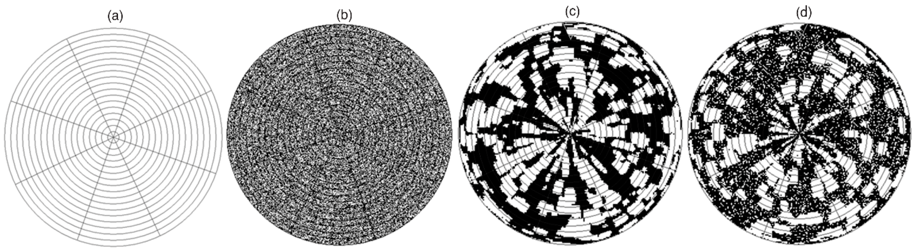
2.4. Angular Simulations to Test the Angular Grid Algorithm

A sensitivity analysis was carried out using simulated TLS angular data to evaluate the performance of the angular grid algorithm to retrieve GF. To model variations found in the actual TLS data, this analysis considered several sources: the angular resolution and its noise, the gap spatial pattern distribution and the amount of GF itself.

A multivariate normal distribution function in Matlab R2017b (The Mathworks; Natick, MA, USA; www.mathworks.com) mimicked the angular noise produced by the mechanical components of the TLS head, which was considered the same for θ and ϕ directions. Such uncertainty is a function of (1) the noise amplitude that was modeled as a percentage of its angular resolution; (2) its variance (noise²) and (3) its covariance (zero) in θ and ϕ directions. The covariance is considered zero because theoretically the uncertainty in θ should not influence the uncertainty in ϕ. Another source of variation consisted in modeling several canopy gap spatial pattern distributions, such as random gaps (R), clusters of gaps (C) and a combination of both (RC) (Figure 3). The GF was increased by progressively removing laser pulses within each gap pattern. For the R pattern, random index numbers in Matlab removed pulses individually without replacement. The C gap pattern randomly identified a coordinate in the angular space and from this position, a convex hull function fitted a circle with a dynamic random radius ranging from one to ten times the angular resolution and removed all laser pulses within it.

The RC gap pattern combined a proportion of 30% R and 70% C gaps. Following these gap patterns, 1890 simulations were generated from 10 replicas with 2–14% noise every 2%; 0.1–0.9 GF every 0.1; and R, C and RC gap patterns. Given that this simulated dataset contained a pre-defined known angular resolution and GF, it was considered as reference to validate the GF algorithm. A Kruskal-Wallis non-parametric distribution test evaluated the algorithm sensitivity to the noise and to the GF spatial patterns in relation to the GF estimations following Hollander and Wolfe [44].

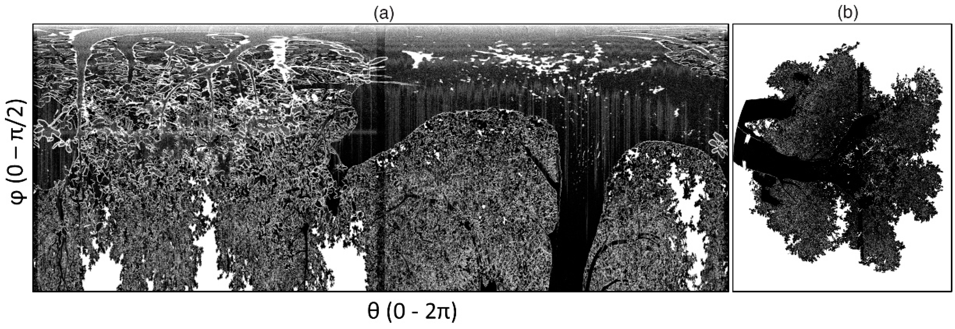
Simulated Hemispherical Images

The Sim-TLS data were converted into SHI (Sim-TLS-SHI) to compare the GF estimates from HI and from the angular grid algorithm. The analysis of HI is one of the most widely accepted indirect methods to estimate GF [5,45]. A 2 to 6% noise level was selected to build the Sim-TLS-SHI that ensured an accurate GF estimate for all three gap patterns (see results section). The Sim-TLS-SHI produces a projection of a hemisphere in a plane. The simplest and most common hemispherical lens geometries are the polar and equiangular projection [6,35]. The following polar transformation was applied:

$$l=2R\phi /\pi$$

(1)

where R is the radius of the whole field of view in the HI, ranging from 0 to π/2; $\phi$ is the zenith angle, which can be understood as the angle between a point in the scene and the optical axis; and l is the radial distance from the optical axis on the HI image.

Since this projection is comparable to actual HI, Seidel et al. [22] and Cifuentes et al. [20] applied it to simulate HI from TLS voxels. Due to this transformation, each pixel on the Sim-TLS-SHI image could include more than one return and/or gap from the angular data (Figure 4). Therefore, the algorithm presented here recorded the number of laser returns and gaps contained within each Sim-TLS-SHI pixel. If the laser return to gap ratio was ≥0.5, the pixel was considered a return (DN = 0) and below this threshold a gap (DN = 255), to record them in 8 bits TIF format images. Hemiview v2.1 software (Delta-T Devices, UK, www.delta-t.co.uk) processed the Sim-TLS-SHI dividing the skymap in 8 θ and 18 ϕ sections (Figure 5). The number of sections in the skymap must be a compromise of the following criteria for a reliable GF estimate: (1) low enough so that GF statistics are meaningful and also invertible; (2) high enough so that the assumption of randomness of leaf distribution within a skymap section remains valid [46]. Taking these two factors into account, the skymap contained 144 sections with a minimum of ten pixels in each one. Finally, a fixed 128 threshold value segmented the Sim-TLS-SHI to compute GF.

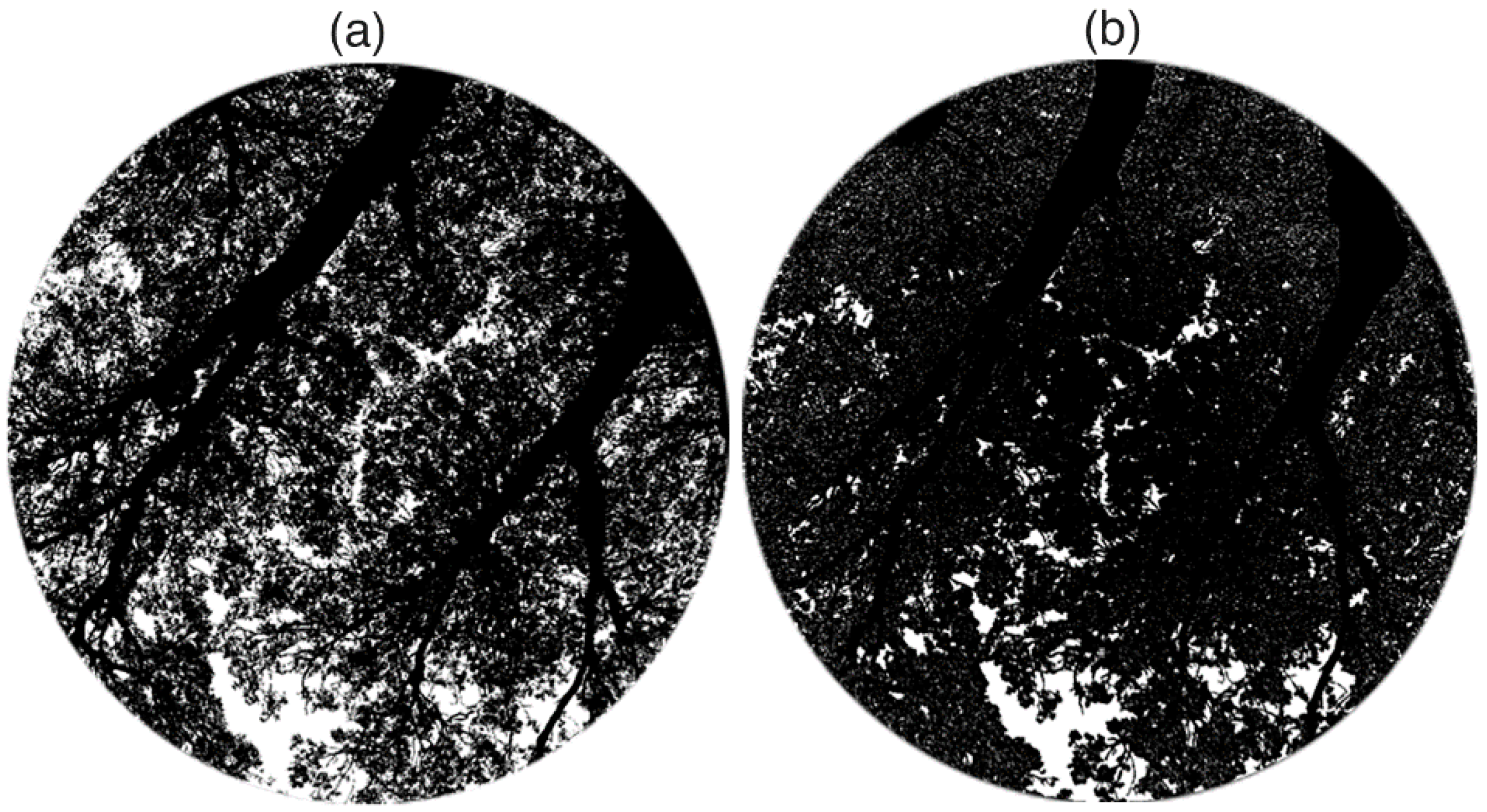
2.5. Application of the Angular Grid Algorithm to Actual TLS Data

After testing the angular grid algorithm to estimate GF over the simulated angular dataset, it was applied to actual TLS data acquired over the holm oak trees in the study area in Las Majadas del Tietar. Cyclone v6.0 software (Leica Geosystems) generated the point cloud for each of the eight TLS samples. Following Seidel et al. [22], Cyclone only considered data with 0.01–1.0 laser intensity, <80 m range and >1.6 mm distance between laser returns. Subsequently, the TLS point cloud surrounding the center of the tree canopy was selected and exported as XYZ ASCII files. TLS XYZ ASCII data were transformed to compute spherical coordinates (θ, ϕ) of each return. Given the large data volume and based on previous works [36,47], ~1° ϕ slices divided the TLS angular data to facilitate further processing. As previously described in Section 2.1, the angular resolution was computed for each slice. Furthermore, the final angular resolution was the average of all ϕ slices, excluding slices located between 0 and 6° ϕ. For these slices, the lower number of laser returns and the distances collected by the angular algorithm produced abnormal angular resolution values (see Results Section 3.2).

To verify the TLS angular resolution, this work extracted manually a small tree trunk section without gaps from each TLS sample with laser pulse density and at a range comparable to the tree canopy. A visual exploratory analysis checked for inconsistencies due to gaps in the trunk section or due to TLS oversampling before computing its angular resolution and noise. Similarly to the simulated data, GF was computed for TLS canopy data using the angular grid that contained the presence/absence of laser returns. To compare with the conventional GF estimation from HI, each TLS canopy sample was transformed into SHI (TLS-SHI) to calculate GF in Hemiview (Figure 6).

In regards to the actual HI, a 0–60° ϕ angular range constriction avoided fuzzy pixels that would comprise a mix of vegetation canopy and sky information [6]. In addition, this constriction was necessary to select a common ϕ range between HI and TLS, since the smaller camera sensor cropped the fisheye FOV to 120° [48]. Hemiview processed only the HI blue channel, since it provides the maximum contrast between canopy objects and sky [49]. As Jonckheere et al. [50] described, manual HI thresholding is a subjective and challenging task to reproduce consistently that can introduce an additional error to the GF computation. For this, the automatic thresholding developed by Ridler and Calvard [11] classified the pixels in the HI as canopy (black) or sky (white). This method finds the midpoint between two clusters by iteratively estimating the average of two cluster means. This approach performed best in a comparison of different thresholding methods to compute GF automatically from HI [50]. It also did better in lighter than darker illumination conditions, as it was the case here. Even though it was developed to process HI at the plot level, it also should work for individual trees as long as the gaps of the outer tree limit are previously masked out and the HI quality warranties the distinction between the two clusters. Masking was unnecessary here since the goal was the comparison between HI and TLS within their previously selected common region. After visual inspection, results were consistent throughout the eight HI and the method was preferred over the subjective manual HI thresholding.

3. Results

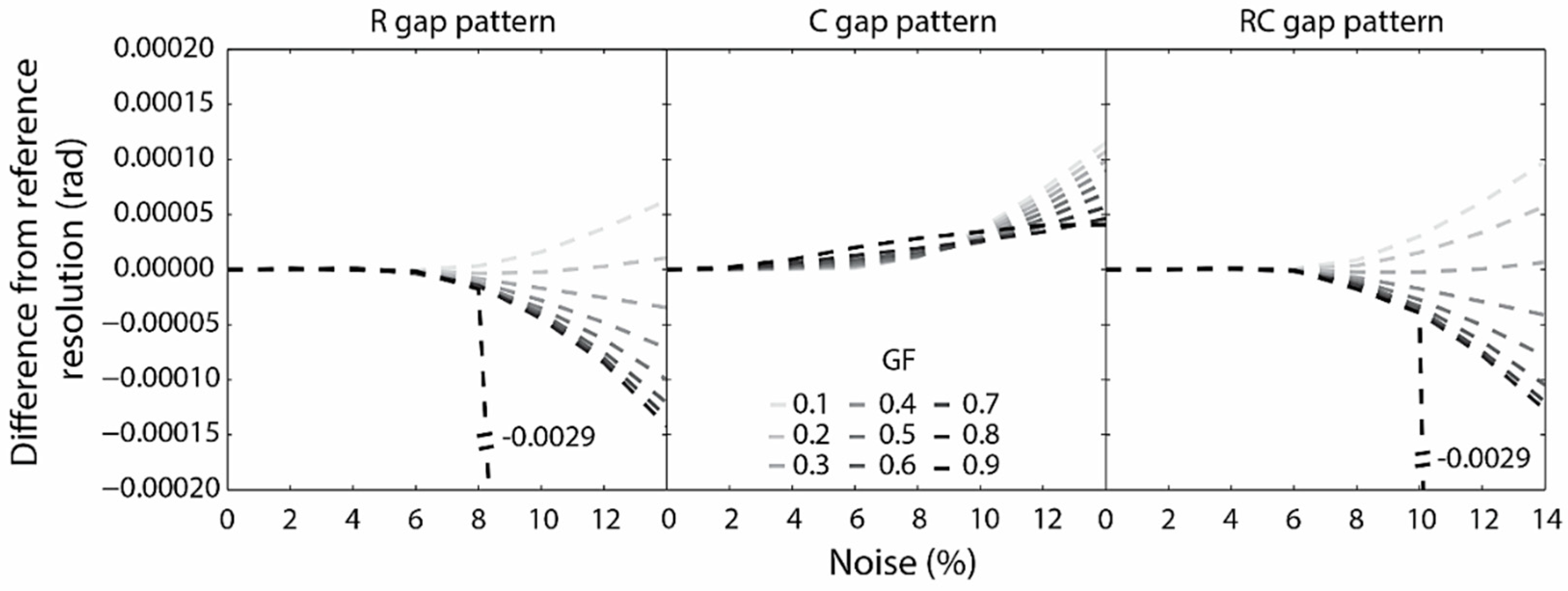
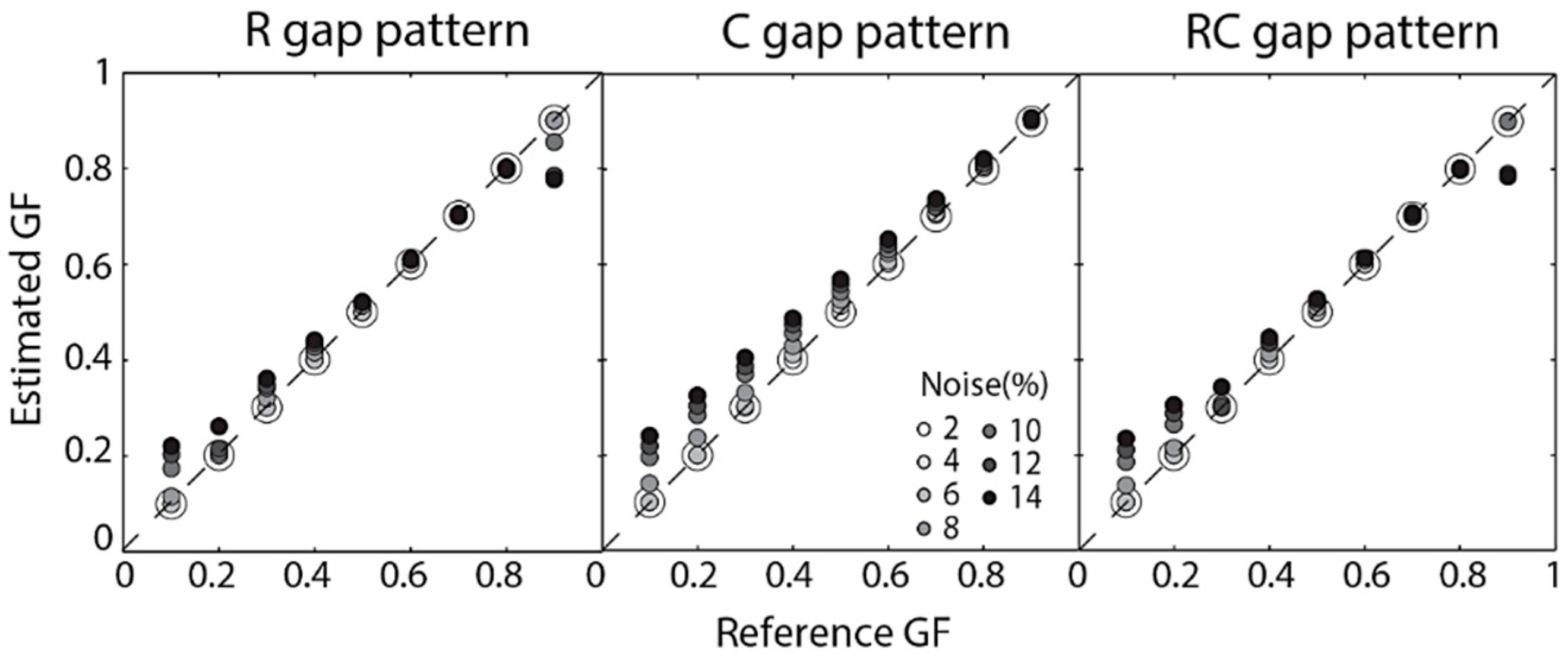
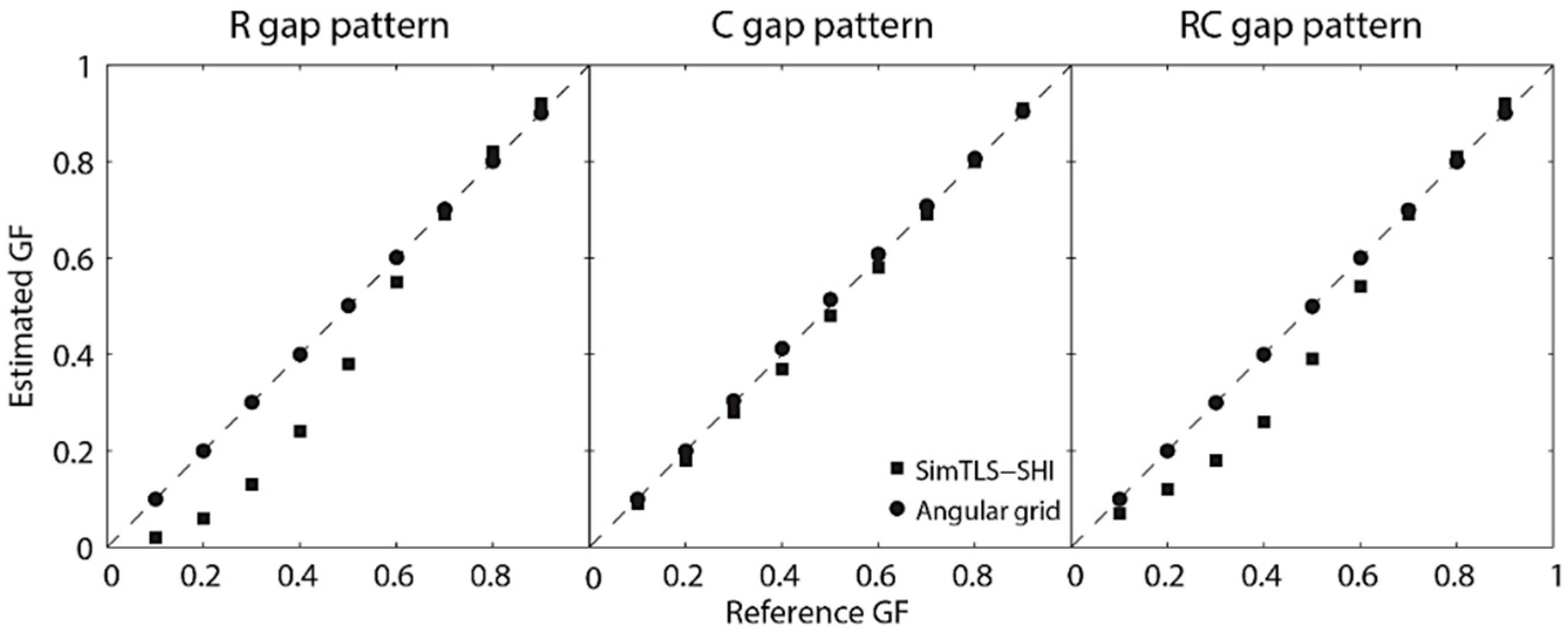
3.1. Simulated Angular Data: Angular Resolution, GF and Sim-TLS-SHI

Figure 7 shows the differences between the reference angular resolution and the computed by the algorithm for the R, C and RC gap patterns with 0.1–0.9 GF and 0–14% noise. R and RC gap patterns kept resolution values closer to the reference if noise remained <6%. C gap pattern instead obtained good resolutions only for <4%. Above 6% noise, the R and RC gap patterns provided coarser resolutions, except for GF data between 0.1 and 0.2, whereas C gap pattern retrieved values finer than the reference.

GF showed a close to zero average difference with the reference for 2–6% noise values for all the simulated gap patterns (Figure 8). The C gap pattern systematically provided higher differences with reference GF for 4–14% noise than R and RC gap patterns, except for 0.9 GF. The Kruskal-Wallis’s test applied over each gap pattern in the simulated dataset indicated that GF estimates are all sensitive to the noise (p-values<0.01), except the R and RC gap patterns with 0.8 GF, which did not show significant differences. The test also showed that the gap patterns did not influence the GF calculation if the noise remained <6% of the angular resolution, except for the C gap pattern. In this gap pattern, the 0.4–0.8 GF presented differences with the GF estimated from R and RC patterns. For higher noise, the test indicated that there were differences between the reference GF and the computed one for all gap patterns (

Table 2. Statistical differences (p-value < 0.01 *) according to the KW test between angular grids with R, C and RC gap patterns, 2–14% noise and 0.1-0.9 GF.

	GF	0.1	0.2	0.3	0.4	0.5	0.6	0.7	0.8	0.9
Noise
2%		()	()	()	()	()	()	()	()	()
4%		()	()	()	()	()	()	()	()	()
6%		()	()	()	(*)	(*)	(*)	(*)	(*)	()
8%		(*)	(*)	(*)	(*)	(*)	(*)	(*)	(*)	(*)
10%		(*)	(*)	(*)	(*)	(*)	(*)	(*)	(*)	(*)
12%		(*)	(*)	(*)	(*)	(*)	(*)	(*)	(*)	(*)
14%		(*)	(*)	(*)	(*)	(*)	(*)	(*)	(*)	(*)

). Regarding the comparison between GF from the angular grids and from Sim-TLS-SHI, the C gap pattern obtained the best agreement with a 2% average difference, followed by RC with 6% and R with 8% (Figure 9).

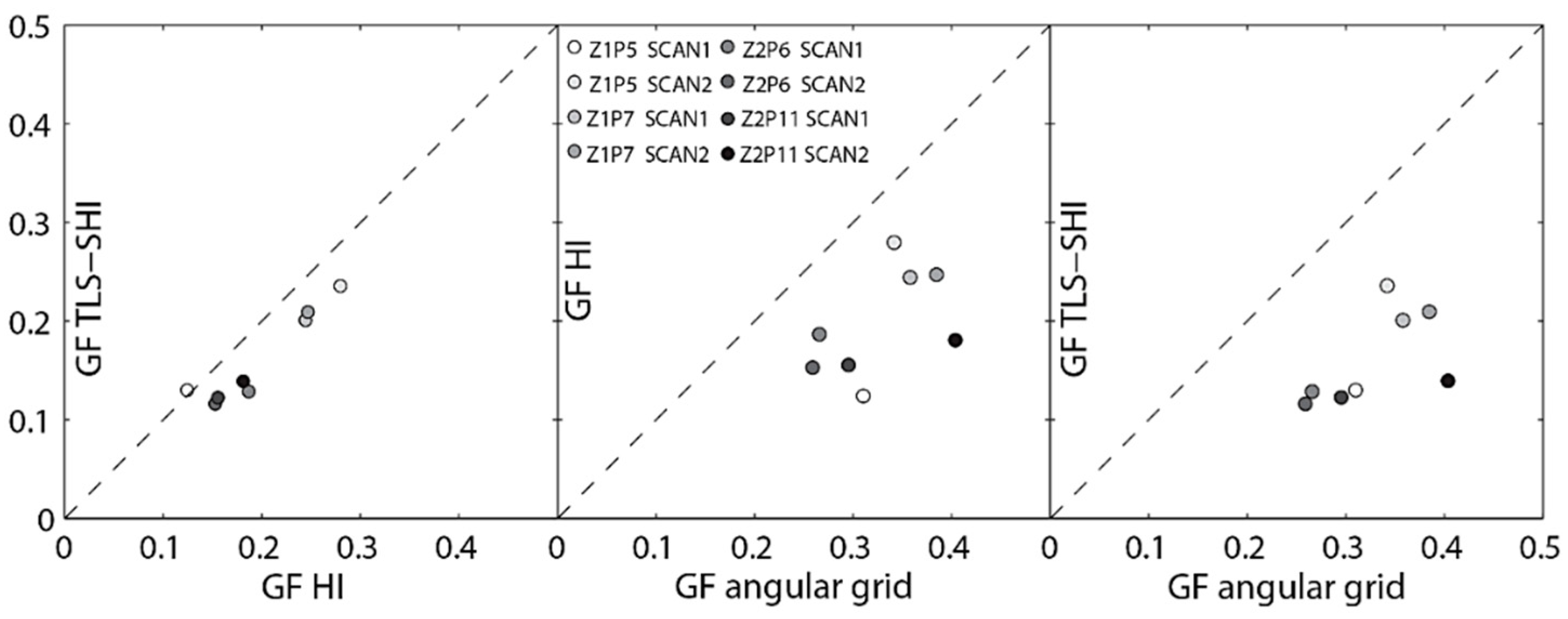
3.2. Actual TLS Angular Data: Angular Resolution, GF and TLS-SHI

Computation of the angular resolution for the actual TLS data yielded an average value of 6.28 × 10⁻⁴ rad for both the θ and ϕ, whereas the noise was 5.77% and 3.17% of the angular resolution, respectively (

Table 3. Tree ID, angular resolution, noise and GF for TLS tree data.

Tree ID	Resolution θ (rad)	Noise θ (%)	Resolution ϕ (rad)	Noise ϕ (%)	GF
Z1P5_SCAN1	6.28 × 10−4	6.11	6.28 × 10−4	2.90	0.31
Z1P5_SCAN2	6.28 × 10−4	5.80	6.28 × 10−4	3.12	0.34
Z1P7_SCAN1	6.28 × 10−4	5.74	6.28 × 10−4	2.58	0.36
Z1P7_SCAN2	6.28 × 10−4	6.31	6.28 × 10−4	3.36	0.38
Z2P6_SCAN1	6.28 × 10−4	5.29	6.28 × 10−4	3.01	0.27
Z2P6_SCAN2	6.28 × 10−4	5.68	6.28 × 10−4	2.85	0.26
Z2P11_SCAN1	6.28 × 10−4	5.45	6.28 × 10−4	3.06	0.30
Z2P11_SCAN2	6.28 × 10−4	5.76	6.28 × 10−4	4.46	0.40
AVERAGE	6.28 × 10−4	5.77	6.28 × 10−4	3.17	0.33

). GF estimated from the angular grid ranged between 0.26 and 0.40, with a 0.33 average. After processing the trunks data, they revealed a very similar angular resolution of 6.28 × 10⁻⁴ rad for both the θ and ϕ, whereas the noise decreased to 4.43% and 1.27% of the angular resolution, respectively (

Table 4. Trunk ID, angular resolution and noise computed for TLS trunk data.

Trunk ID	Resolution θ (rad)	Noise θ (%)	Resolution ϕ (rad)	Noise ϕ (%)
Z1P5_SCAN1	6.27 × 10−4	4.43	6.29 × 10−4	1.29
Z1P5_SCAN2	6.28 × 10−4	4.22	6.29 × 10−4	1.18
Z1P7_SCAN1	6.27 × 10−4	5.07	6.28 × 10−4	1.29
Z1P7_SCAN2	6.28 × 10−4	4.99	6.28 × 10−4	1.27
Z2P6_SCAN1	6.28 × 10−4	4.11	6.29 × 10−4	1.24
Z2P6_SCAN2	6.28 × 10−4	4.63	6.28 × 10−4	1.27
Z2P11_SCAN1	6.27 × 10−4	3.57	6.29 × 10−4	1.53
Z2P11_SCAN2	6.28 × 10−4	4.39	6.28 × 10−4	1.11
AVERAGE	6.28 × 10−4	4.43	6.28 × 10−4	1.27

). Besides, ϕ TLS slices close to the zenith (0°) achieved erroneous average resolutions, especially for θ with 6.56 × 10⁻⁴ rad and 18.07% noise (

Table 5. Noisy ϕ slices for each Tree ID, computed angular resolution and noise.

Tree ID	Slice ϕ (°)	Resolution θ (rad)	Noise θ (%)	Resolution ϕ (rad)	Noise ϕ (%)
Z1P5_SCAN1	0–6	6.76 × 10−4	19.05	6.27 × 10−4	3.18
Z1P5_SCAN2	0–3	6.53 × 10−4	17.97	6.27 × 10−4	3.05
Z1P7_SCAN1	0–2	6.78 × 10−4	19.62	6.27 × 10−4	2.99
Z1P7_SCAN2	0–3	6.61 × 10−4	19.10	6.27 × 10−4	3.01
Z2P6_SCAN1	0–3	6.29 × 10−4	13.87	6.27 × 10−4	3.02
Z2P6_SCAN2	0–2	6.43 × 10−4	17.33	6.27 × 10−4	2.75
Z2P11_SCAN1	0–2	6.61 × 10−4	19.55	6.27 × 10−4	3.13
Z2P11_SCAN2	0–3	6.46 × 10−4	18.04	6.27 × 10−4	2.96
AVERAGE		6.56 × 10−4	18.07	6.27 × 10−4	3.01

). The number of erroneous slices also varied by scan. In regards to TLS-SHI, Figure 10 shows an example of an angular grid image and its transformation to TLS-SHI. The TLS-SHI underestimated GF by an average of 4% compared to HI (Figure 11a). HI and TLS-SHI presented 14% and 17% lower values than the GF calculated from the angular grids, respectively (Figure 11b,c).

4. Discussion

4.1. Angular Resolution and GF

The algorithm estimates accurately the angular resolution on simulated angular data when the noise is <6% (Figure 7). Beyond this noise level, GF becomes unreliable for all the gap patterns, especially for C (Table 2). Since the angular grid uses the computed angular resolutions, an erroneous higher angular resolution originates a grid with an excessive number of cells that are not possible to fill with laser returns, creating false gaps that overestimate GF (Figure 8). This C gap pattern has a higher chance of selecting groups of neighbor returns closer to each other that will produce a higher angular resolution. In addition, the probability of selecting returns coming from non-neighbor pulses notoriously increases for GF > 0.8, especially for R and RC. The distance between returns augments and so it decreases the angular resolution (Figure 7). As a result, an angular grid with fewer cells reduces the chance of having gaps and thus underestimates GF. This situation is noticeable for extreme simulation scenarios with 10–14% noise and GF > 0.80 (Figure 8).

The algorithm proposed here would potentially work at the plot level, even though it was developed for individual trees if the noise in the data remains <6%. A plot of trees with high LAI but large gaps in between them that behaves more like a C gap pattern would produce good results even over 0.8 GF. On the contrary, a plot of trees with low LAI and large gaps in between them, more like RC, or homogenously distributed trees with very low LAI, more like R, would fail over 0.80 GF, due to the lack of enough neighbor returns to calculate the angular resolution.

Table 3 and Table 4, confirmed the initial assumption that the angular resolution is the same in θ and ϕ for the actual TLS data, with <1.00 × 10⁻⁶ rad difference in all cases. Therefore, taking the average of θ and ϕ demonstrated to be accurate to calculate the angular resolution. To estimate this resolution, the algorithm requires having neighbor returns. Consequently, if neighbor returns are subject to higher noise, or if there are enough isolated returns without any neighbors, the algorithm will fail to deliver GF adequately. This is evident in the 0–6° ϕ TLS slices that provided different average resolutions values, especially for θ, with 6.56 × 10⁻⁴ rad and noise of 18.07% (Table 5 and Figure 10a upper part). The distribution of the elements on the crown architecture and TLS θ spin is too narrow at these ϕ slice range to sample enough neighbor returns. However, as soon as the algorithm collected more returns with suitable neighbors, it could compute the right resolution. Given that the angular resolution is expected constant for the whole hemisphere, excluding the ϕ slices with problems determines the angular resolution correctly.

The TLS Leica HDS-6000 manufacturer reports a priori an angular noise value of 1.25 × 10⁻⁴ rad, but the actual noise observed in this study was lower, 2.78 × 10⁻⁵ rad (4.43%) in θ and 7.97 × 10⁻⁶ rad (1.27%) in ϕ for the tree trunks (Table 4); and 3.62 × 10⁻⁵ (5.77%) in θ and 1.99 × 10⁻⁵ (3.17%) in ϕ for the overall trees (Table 3). This noise is optimal for the GF estimation using angular grids since the algorithm performed consistently well for these noise levels for all conditions tested on simulated TLS angular data (Figure 7, Figure 8 and Figure 9). Other studies have demonstrated also lower noise values than reported a priori by the manufacturer. For example, Kremen et al. [37] estimated 4.70 × 10⁻⁵ rad deviations in both θ and ϕ; and Reshetyuk [38] found 2.79 × 10⁻⁵ and 1.57 × 10⁻⁵ rad in θ and ϕ with a Leica HDS-3000 TLS system. The difference between horizontal and vertical deviations can be attributed to the mechanism in the TLS that produces the angular sampling [51]. In this work, the accuracy of ϕ was about twice as good as θ, probably because according to Reshetyuk [38] the scanning mirror that rotates vertically produces lower inertia than the servomotor that rotates horizontally.

The TLS Leica HDS-6000 collects data forward and backward using a spin of 182° instead of 180°. Therefore, it oversamples 4° in the θ direction (see Figure 10a, central θ values). Leica Geosystems technical support confirmed this fact in a personal communication. This problem could be identified and considered with the angular grid method, since the estimated angular resolution was higher for this 4° θ section (data no shown) than the overall value. Danson et al. [27] and Ramírez et al. [28] calculated GF as a ratio of the non-returns to the total number of laser pulses emitted using the theoretical resolution of the instrument. In their case, the oversampling error would be overlooked since their method cannot determine where exactly this oversampling occurs. This issue causes a higher ratio between returns and total number of pulses emitted and, consequently, a lower GF.

Additional problems might also appear when a laser beam hits a canopy object, because the strength of the reflected signal depends on several factors that includes the reflection coefficient, surface roughness, the incidence angle and the fraction of the pulse cross section covered by the target [30]. As a result, it seems the edge of the canopy objects will lack of laser returns and assumed as gaps in the angular grid. Vegetation canopies also contain complex discontinuous rough elements with particular reflectance properties for which pulses do not always reflect properly back to the TLS providing noisy returns, such as in trunks (see gaps in Figure 10a), branches and leaves [20,52,53]. The noisy returns especially appear in phase instruments [20] and the filter applied does not guarantee to remove them completely.

4.2. Simulation of Hemispherical Images

Sim-TLS-SHI underestimated GF especially for 0.1–0.5 GF (Figure 9). Average differences in this range reached 9% for RC gap pattern and 14% for R. The deformation caused by the polar projection and the method used to classify the pixels can explain in part these lower GF values. The polar projection transforms each point keeping true the direction and exact distance from the projection center point, whereas all other directions and distances are deformed. In consequence, the area distortion and shapes increase as it moves away from the center [54]. As a result, pixels in the center zone and in the outer border of the image contain more laser returns that reduces the chance to find gaps and hence underestimates GF (Figure 4b). This problem is exacerbated for the R and RC gap patterns, because small or individual random gaps could be part of pixel groups formed by several returns, masking such gaps (Figure 5).

The TLS-SHI slightly underestimated GF compared to HI (Figure 11a). Calders et al. [26], Ramírez et al. [28], Seidel et al. [22], Cifuentes et al. [20] also demonstrated this under estimations for a similar ϕ range. HI and TLS-SHI achieved much lower GF than the angular grid (Figure 11b). The angular grid does not project the data and the GF is computed on a cell basis for the whole image. Having HI and TLS-SHI the same polar projection explains their closer agreement in GF estimates. The mismatch with the angular grid does not actually mean that its result is necessarily worse. Actually, transforming the angular grid to TLS-SHI loses information for many TLS-SHI pixels that contain multiple laser pulses (Figure 4b). These pixels only record a return or a gap based on the laser return to gap ratio. As it was seen for the Sim-TLS-SHI, the effect of re-projecting caused a systematic GF underestimation, which is noticeable in R and RC gap patterns with lower GF values (Figure 9). On top of these differences, the lack of returns in the canopy objects edge, could contribute to a GF increase in the angular grids.

GF from TLS-SHI was an average 4% smaller than the one from HI (Figure 11a). The correlation between them (R² = 0.89) is in concordance with the R² = 0.76 obtained by Seidel et al. [22] in a forest with large gaps. However, Kuusk et al. [30] point out that the HI overestimation, between 10 and 20% even in optimal light conditions, causes part of this GF underestimation. The HI is widely used to compute GF, but the processing generally does not take into account the specular reflection of the sky on the foliage, which depends on LAI and leaf angle distribution (LAD) [55]. The HI were not always taken under optimal light conditions and sky light illumination was too bright causing blooming effects in parts of the HI. For example, small and thin branches were not visible in the classified HI, even when they appear in the original ones [22].

Although canopy geometry is well depicted by both approaches (Figure 6), small gaps clearly visible in HI seemed to be smaller or even disappear in the TLS-SHI. This effect is related to the 0.22 mrad laser beam divergence that translates into a ~5 mm footprint at 8 m from the TLS. Therefore, the TLS will not be able to detect gaps smaller than this size. According to Danson et al. [56], if a gap occupying less than 50% of the laser beam is detected by the TLS and this will lead to underestimation of GF. In this respect, canopies with large gaps seem to be more suitable to characterize GF from TLS [22].

Likewise, the experiment here preferred to analyze each scan separately, since the objective was to have enough samples to test an algorithm to estimate GF at the full TLS resolution. The co-registration from several scans increases the quality of TLS phase data and would improve the representation of the elements [20]. In any case, it was necessary to select a common angular section for both sensors since the field of view of the TLS and the HI camera were not exactly the same. Matching both images was carried out visually, to obtain all processed ϕ sectors coincident in the angular space. This selection also adds uncertainty that contributes to the differences between GF values obtained from both instruments.

HI analysis to retrieve GF is a mature technology. Contrary to TLS, it requires very cheap equipment and available tools can quickly process HI. In addition, data acquisition is faster, and operators do not require advanced training. Some drawbacks are the short time window recommended for measurements: right before dawn, right after dusk or under overcast skies [57]. But even under these circumstances, using HI to track changes over natural vegetation is challenging and dependent on the precision of the subjective/automatic canopy/sky threshold. Other important issue is the specular reflection phenomenon that affects the HI and produces a considerable overestimation in GF. Contrary, TLS is a relatively new technology that has the potential to highly impact the detailed measurement of canopy structure [18]. Since TLS is independent of light conditions, it provides more consistent data than HI. However, most of the TLS comes from civil applications and they were designed to measure hard objects, like buildings or terrain, not soft objects, like vegetation canopies. This issue presents challenges that require the development of optimal processing tools.

5. Conclusions

A new method to estimate GF from TLS data was proposed and validated. The algorithm adjusts an angular grid to compute the angular resolution and calculates GF from the proportion of empty grid cells without laser returns. By working with spherical instead of Cartesian coordinates, the results are independent from the distance between laser returns and the position of the TLS. The method performed satisfactory over the simulated angular data when the noise did not exceed 6%. The C gap pattern showed higher differences compared to the reference data than the other two gap patterns. The excessive noisy angular returns cause an overestimation of the angular resolution that increases the number of cells in the grid, creating false gaps and overestimating GF. Actual TLS revealed lower noise than the manufacturer indicated a priori. This noise level is within the accurate performance of the angular grid algorithm. Sim-TLS-SHI presented a systematic underestimation of the GF that affected especially R and RC gap patterns. Angular data transformation into HI causes a direction deformation in the new coordinate system that requires further research. TLS-SHI showed lower GF values than HI, which are affected by footprint size and the specular reflection. An advantage of the proposed method is that it provides spatial information on the gap distribution, which is of great importance for the analysis of light regimes. It also provides accurate information at the full TLS resolution on the gap distribution and the gap size distribution from which measures of clumping index can be derived. The algorithm was tested on individual trees, but it could work at plot level to characterize canopy gaps. Over 0.8 GF, it would fail if neighbor returns are insufficient to properly estimate the angular resolution.

References

1. Soma, M.; Pimont, F.; Durrieu, S.; Dupuy, J.-L. Enhanced Measurements of Leaf Area Density with T-LiDAR: Evaluating and Calibrating the Effects of Vegetation Heterogeneity and Scanner Properties. Remote Sens. 2018, 10, 1580. [Google Scholar] [CrossRef] [Green Version]
2. Vezy, R.; Christina, M.; Roupsard, O.; Nouvellon, Y.; Duursma, R.; Medlyn, B.E.; Soma, M.; Charbonnier, F.; Blitz-Frayret, C.; Stape, J.-L.; et al. Measuring and modelling energy partitioning in canopies of varying complexity using MAESPA model. Agric. For. Meteorol. 2018, 253, 203–217. [Google Scholar] [CrossRef]
3. Dassot, M.; Constant, T.; Fournier, M. The use of terrestrial LiDAR technology in forest science: Application fields, benefits and challenges. Ann. For. Sci. 2011, 68, 959–974. [Google Scholar] [CrossRef] [Green Version]
4. Chen, J.M.; Black, T.A. Defining leaf area index for non-flat leaves. Plant Cell Environ. 1992, 15, 421–429. [Google Scholar] [CrossRef]
5. Welles, J.M.; Cohen, S. Canopy structure measurement by gap fraction analysis using commercial instrumentation. J. Exp. Bot. 1996, 47, 1335–1342. [Google Scholar] [CrossRef]
6. Jonckheere, I.; Fleck, S.; Nackaerts, K.; Muys, B.; Coppin, P.; Weiss, M.; Baret, F. Review of methods for in situ leaf area index determination: Part I. Theories, sensors and hemispherical photography. Agric. For. Meteorol. 2004, 121, 19–35. [Google Scholar] [CrossRef]
7. Weiss, M.; Baret, F.; Smith, G.J.; Jonckheere, I.; Coppin, P. Review of methods for in situ leaf area index (LAI) determination: Part II. Estimation of LAI, errors and sampling. Agric. For. Meteorol. 2004, 121, 37–53. [Google Scholar] [CrossRef]
8. Gonsamo, A.; Pellikka, P. Methodology comparison for slope correction in canopy leaf area index estimation using hemispherical photography. For. Ecol. Manag. 2008, 256, 749–759. [Google Scholar] [CrossRef]
9. Leblanc, S.G.; Chen, J.M.; Fernandes, R.; Deering, D.W.; Conley, A. Methodology comparison for canopy structure parameters extraction from digital hemispherical photography in boreal forests. Agric. For. Meteorol. 2005, 129, 187–207. [Google Scholar] [CrossRef] [Green Version]
10. Frazer, G.W.; Fournier, R.A.; Trofymow, J.; Hall, R.J. A comparison of digital and film fisheye photography for analysis of forest canopy structure and gap light transmission. Agric. For. Meteorol. 2001, 109, 249–263. [Google Scholar] [CrossRef]
11. Ridler, T.; Calvard, S. Picture thresholding using an iterative selection method. IEEE Trans. Syst. Man Cybern. 1978, 8, 630–632. [Google Scholar] [CrossRef]
12. Olsson, L.; Carlsson, K.; Grip, H.; Perttu, K. Evaluation of forest-canopy photographs with diode-array scanner OSIRIS. Can. J. For. Res. 1982, 12, 822–828. [Google Scholar] [CrossRef]
13. Lang, M.; Kuusk, A.; Mõttus, M.; Rautiainen, M.; Nilson, T. Canopy gap fraction estimation from digital hemispherical images using sky radiance models and a linear conversion method. Agric. For. Meteorol. 2010, 150, 20–29. [Google Scholar] [CrossRef]
14. Wehr, A.; Lohr, U. Airborne laser scanning—An introduction and overview. ISPRS J. Photogramm. Remote Sens. 1999, 54, 68–82. [Google Scholar] [CrossRef]
15. Lichti, D.; Jamtsho, S. Angular resolution of terrestrial laser scanners. Photogramm. Rec. 2006, 21, 141–160. [Google Scholar] [CrossRef]
16. Newnham, G.J.; Armston, J.D.; Calders, K.; Disney, M.I.; Lovell, J.L.; Schaaf, C.B.; Strahler, A.H.; Danson, F.M. Terrestrial laser scanning for plot-scale forest measurement. Curr. For. Rep. 2015, 1, 239–251. [Google Scholar] [CrossRef] [Green Version]
17. Calders, K.; Newnham, G.; Burt, A.; Murphy, S.; Raumonen, P.; Herold, M.; Culvenor, D.; Avitabile, V.; Disney, M.; Armston, J.; et al. Nondestructive estimates of above-ground biomass using terrestrial laser scanning. Methods Ecol. Evol. 2014, 6, 198–208. [Google Scholar] [CrossRef]
18. Li, Y.; Guo, Q.; Su, Y.; Tao, S.; Zhao, K.; Xu, G. Retrieving the gap fraction, element clumping index, and leaf area index of individual trees using single-scan data from a terrestrial laser scanner. ISPRS J. Photogramm. Remote Sens. 2017, 130, 308–316. [Google Scholar] [CrossRef]
19. Pueschel, P.; Newnham, G.; Hill, J. Retrieval of Gap Fraction and Effective Plant Area Index from Phase-Shift Terrestrial Laser Scans. Remote Sens. 2014, 6, 2601–2627. [Google Scholar] [CrossRef] [Green Version]
20. Cifuentes, R.; Van Der Zande, D.; Farifteh, J.; Salas-Eljatib, C.; Coppin, P. Effects of voxel size and sampling setup on the estimation of forest canopy gap fraction from terrestrial laser scanning data. Agric. For. Meteorol. 2014, 194, 230–240. [Google Scholar] [CrossRef]
21. Hancock, S.; Essery, R.; Reid, T.; Carle, J.; Baxter, R.; Rutter, N.; Huntley, B. Characterising forest gap fraction with terrestrial lidar and photography: An examination of relative limitations. Agric. For. Meteorol. 2014, 189, 105–114. [Google Scholar] [CrossRef] [Green Version]
22. Seidel, D.; Fleck, S.; Leuschner, C. Analyzing forest canopies with ground-based laser scanning: A comparison with hemispherical photography. Agric. For. Meteorol. 2012, 154, 1–8. [Google Scholar] [CrossRef]
23. Zheng, G.; Moskal, L.M. Computational-Geometry-Based Retrieval of Effective Leaf Area Index Using Terrestrial Laser Scanning. IEEE Trans. Geosci. Remote Sens. 2012, 50, 3958–3969. [Google Scholar] [CrossRef]
24. Lovell, J.; Jupp, D.; Culvenor, D.S.; Coops, N.C. Using airborne and ground-based ranging lidar to measure canopy structure in Australian forests. Can. J. Remote Sens. 2003, 29, 607–622. [Google Scholar] [CrossRef]
25. Wilkes, P.; Lau, A.; Disney, M.; Calders, K.; Burt, A.; De Tanago, J.G.; Bartholomeus, H.; Brede, B.; Herold, M. Data acquisition considerations for Terrestrial Laser Scanning of forest plots. Remote Sens. Environ. 2017, 196, 140–153. [Google Scholar] [CrossRef]
26. Calders, K.; Verbesselt, J.; Bartholomeus, H.M.; Herold, M. Applying terrestrial LiDAR to derive gap fraction distribution time series during bud break. In Proceedings of the SilviLaser 2011, 11th international LiDAR Forest Applications Conference, Hobart, Australia, 16–20 October 2011. [Google Scholar]
27. Danson, F.M.; Hetherington, D.; Koetz, B.; Morsdorf, F.; Allgöwer, B. Forest Canopy Gap Fraction From Terrestrial Laser Scanning. IEEE Geosci. Remote Sens. Lett. 2007, 4, 157–160. [Google Scholar] [CrossRef] [Green Version]
28. Ramírez, A.; Armitage, R.; Danson, F.M. Testing the Application of Terrestrial Laser Scanning to Measure Forest Canopy Gap Fraction. Remote Sens. 2013, 5, 3037–3056. [Google Scholar] [CrossRef] [Green Version]
29. Vaccari, S.; Van Leeuwen, M.; Calders, K.; Coops, N.C.; Herold, M. Bias in lidar-based canopy gap fraction estimates. Remote Sens. Lett. 2013, 4, 391–399. [Google Scholar] [CrossRef]
30. Kuusk, A.; Pisek, J.; Lang, M.; Gruno, A. Estimation of Gap Fraction and Foliage Clumping in Forest Canopies. Remote Sens. 2018, 10, 1153. [Google Scholar] [CrossRef] [Green Version]
31. Calders, K.; Schenkels, T.; Bartholomeus, H.; Armston, J.; Verbesselt, J.; Herold, M. Monitoring spring phenology with high temporal resolution terrestrial LiDAR measurements. Agric. For. Meteorol. 2015, 203, 158–168. [Google Scholar] [CrossRef]
32. Portillo-Quintero, C.; Sánchez-Azofeifa, G.A.; Culvenor, D.S. Using VEGNET In-Situ Monitoring LiDAR (IML) to Capture Dynamics of Plant Area Index, Structure and Phenology in Aspen Parkland Forests in Alberta, Canada. Forests 2014, 5, 1053–1068. [Google Scholar] [CrossRef]
33. Canham, C.; Denslow, J.S.; Platt, W.J.; Runkle, J.R.; Spies, T.A.; White, P.S. Light regimes beneath closed canopies and tree-fall gaps in temperate and tropical forests. Can. J. For. Res. 1990, 20, 620–631. [Google Scholar] [CrossRef]
34. Hu, L.; Gong, Z.; Li, J.; Zhu, J. Estimation of canopy gap size and gap shape using a hemispherical photograph. Trees 2009, 23, 1101–1108. [Google Scholar] [CrossRef]
35. Gonsamo, A.; Walter, J.-M.N.; Pellikka, P. Sampling gap fraction and size for estimating leaf area and clumping indices from hemispherical photographs. Can. J. For. Res. 2010, 40, 1588–1603. [Google Scholar] [CrossRef]
36. Moorthy, I.; Miller, J.R.; Jimenez-Berni, J.A.; Zarco-Tejada, P.J.; Hu, B.; Chen, J. Field characterization of olive (Olea europaea L.) tree crown architecture using terrestrial laser scanning data. Agric. For. Meteorol. 2011, 151, 204–214. [Google Scholar] [CrossRef]
37. Kremen, T.; Koska, B.; Pospıšil, J. Verification of laser scanning systems quality. In Proceedings of the XXIII FIG Congress, Munich, Germany, 8–13 October 2006; pp. 1–16. [Google Scholar]
38. Reshetyuk, Y. Calibration of Terrestrial Laser Scanners Callidus 1.1, Leica Hds 3000 And Leica Hds 2500. Surv. Rev. 2006, 38, 703–713. [Google Scholar] [CrossRef]
39. Rivas Martínez, S.; Gandullo, J.M. Memoria del Mapa de Series de Vegetación de España: 1: 400.000; ICONA: Madrid, Spain, 1987. [Google Scholar]
40. Luo, Y.; El-Madany, T.S.; Filippa, G.; Ma, X.; Ahrens, B.; Carrara, A.; Gonzalez-Cascon, R.; Cremonese, E.; Galvagno, M.; Hammer, T.W.; et al. Using Near-Infrared-Enabled Digital Repeat Photography to Track Structural and Physiological Phenology in Mediterranean Tree–Grass Ecosystems. Remote Sens. 2018, 10, 1293. [Google Scholar] [CrossRef] [Green Version]
41. Moreno, G.; Pulido, F.J. The Functioning, Management and Persistence of Dehesas. In Agroforestry in Europe; Rigueiro-Rodróguez, A., McAdam, J., Mosquera-Losada, M.R., Eds.; Springer: Dordrecht, The Netherlands, 2008; pp. 127–160. [Google Scholar] [CrossRef]
42. El-Madany, T.S.; Reichstein, M.; Perez-Priego, O.; Carrara, A.; Moreno, G.; Martín, M.P.; Pacheco-Labrador, J.; Wohlfahrt, G.; Nieto, H.; Weber, U.; et al. Drivers of spatio-temporal variability of carbon dioxide and energy fluxes in a Mediterranean savanna ecosystem. Agric. For. Meteorol. 2018, 262, 258–278. [Google Scholar] [CrossRef]
43. Lichti, D.D. A resolution measure for terrestrial laser scanners. Int. Arch. Photogramm. Remote Sens. Spat. Inf. Sci. 2004, 34, 6. [Google Scholar]
44. Hollander, M.; Wolfe, D.A. Nonparametric Statistical Methods, 2nd ed.; John Wiley and Sons: New York, NY, USA, 1999. [Google Scholar]
45. Bréda, N. Ground-based measurements of leaf area index: A review of methods, instruments and current controversies. J. Exp. Bot. 2003, 54, 2403–2417. [Google Scholar] [CrossRef]
46. Lang, A. Estimation of leaf area index from transmission of direct sunlight in discontinuous canopies. Agric. For. Meteorol. 1986, 37, 229–243. [Google Scholar] [CrossRef]
47. Zhen, Z.; Wuming, Z.; Ling, Z.; Jmg, Z. Research on different slicing methods of acquiring LAI from terrestrial laser scanner data. In Proceedings of the 2011 IEEE International Conference on Spatial Data Mining and Geographical Knowledge Services (ICSDM), Fuzhou, China, 29 June–1 July 2011; pp. 295–299. [Google Scholar]
48. García, M.; Gajardo, J.; Riaño, D.; Zhao, K.; Martín, M.P.; Ustin, S. Canopy clumping appraisal using terrestrial and airborne laser scanning. Remote Sens. Environ. 2015, 161, 78–88. [Google Scholar] [CrossRef]
49. Zhao, F.; Yang, X.; Schull, M.A.; Román, M.O.; Yao, T.; Wang, Z.; Zhang, Q.; Jupp, D.; Lovell, J.; Culvenor, D.S.; et al. Measuring effective leaf area index, foliage profile, and stand height in New England forest stands using a full-waveform ground-based lidar. Remote Sens. Environ. 2011, 115, 2954–2964. [Google Scholar] [CrossRef]
50. Jonckheere, I.; Nackaerts, K.; Muys, B.; Coppin, P. Assessment of automatic gap fraction estimation of forests from digital hemispherical photography. Agric. For. Meteorol. 2005, 132, 96–114. [Google Scholar] [CrossRef]
51. Wehr, A. LiDAR: Airborne and terrestrial sensors. In Advances in Photogrammetry, Remote Sensing and Spatial Information Sciences: 2008 ISPRS Congress Book; Li, Z., Chen, J., Baltsavias, E., Eds.; CRC Press: Leiden, The Netherlands, 2008; Volume 7, pp. 73–84. [Google Scholar]
52. Balduzzi, M.A.; Van Der Zande, D.; Stuckens, J.; Verstraeten, W.W.; Coppin, P. The Properties of Terrestrial Laser System Intensity for Measuring Leaf Geometries: A Case Study with Conference Pear Trees (Pyrus communis). Sensors 2011, 11, 1657–1681. [Google Scholar] [CrossRef]
53. Van Der Zande, D.; Stuckens, J.; Verstraeten, W.W.; Mereu, S.; Muys, B.; Coppin, P. 3D modeling of light interception in heterogeneous forest canopies using ground-based LiDAR data. Int. J. Appl. Earth Obs. GeoInf. 2011, 13, 792–800. [Google Scholar] [CrossRef]
54. Maling, D.H. Coordinate Systems and Map Projections, 2nd ed.; Pergamon Press: Oxford, UK, 1992. [Google Scholar]
55. Kuusk, A. Specular reflection in the signal of LAI-2000 plant canopy analyzer. Agric. For. Meteorol. 2016, 221, 242–247. [Google Scholar] [CrossRef]
56. Danson, F.M.; Armitage, R.P.; Bandugula, V.; Ramirez, F.A.; Tate, N.J.; Tansey, K.J.; Tegzes, T. Terrestrial laser scanners to measure forest canopy gap fraction. In Proceedings of the SilviLaser, Edinburgh, UK, 17–19 September 2008; pp. 335–341. [Google Scholar]
57. Riaño, D.; Valladares, F.; Condés, S.; Chuvieco, E. Estimation of leaf area index and covered ground from airborne laser scanner (Lidar) in two contrasting forests. Agric. For. Meteorol. 2004, 124, 269–275. [Google Scholar] [CrossRef]
Figure 1. Flow chart of the methodology applied to carry out this research.
Remotesensing 12 01596 g001
Figure 2. Algorithm to select neighbor laser returns.
Remotesensing 12 01596 g002
Figure 3. Simulated angular data (top) and hemispheric 3D view (bottom) with R (a), C (b) and RC (c) gap patterns and 0.5 GF. The θ range of the top image was constricted for better visualization of the gap patterns.
Remotesensing 12 01596 g003
Figure 4. Simulated angular data with C gap pattern and 0.5 GF for the angular grid method (a) and for its hemispherical transformation (b).
Remotesensing 12 01596 g004
Figure 5. Skymap sectors (a), R (b), C (c) and RC (d) gap patterns for Sim-TLS-SHI.
Remotesensing 12 01596 g005
Figure 6. Actual HI (a) and TLS-SHI from TLS data (b).
Remotesensing 12 01596 g006
Figure 7. Difference between reference angular resolution and the computed one as the average of the θ and ϕ directions.
Remotesensing 12 01596 g007
Figure 8. Comparison between reference and computed GF for R, C and RC gap patterns in the simulated angular data. The 2% noise marker is bigger for visualization purposes.
Remotesensing 12 01596 g008
Figure 9. GF comparison for angular grid and Sim-TLS-SHI images. Data simulated with 6% noise.
Remotesensing 12 01596 g009
Figure 10. Angular grid (a) and its transformation into TLS-SHI (b).
Remotesensing 12 01596 g010
Figure 11. GF comparison between HI and TLS-SHI (a), angular grid and HI (b), and angular grid and TLS-SHI (c).
Remotesensing 12 01596 g011