Deriving VTEC Maps from SMOS Radiometric Data
by
 , , ,
, , ,
Roselena Rubino
1,*, 
Nuria Duffo
1,
Verónica González-Gambau
2,
Ignasi Corbella
1,
Francesc Torres
1,
Israel Durán
1 and
Manuel Martín-Neira
3 1
CommSensLab Research Group, Polytechnic University of Catalonia, c/Jordi Girona 1-3, 08034 Barcelona, Spain
2
Physical Oceanography Department, Institute of Marine Sciences, ICM-CSIC and Barcelona Expert Center, Pg. Marítim de la Barceloneta 37-49, 08034 Barcelona, Spain
3
European Space Research and Technology Center, European Space Agency, 2200 AG Noordwijk, The Netherlands
*
Author to whom correspondence should be addressed.
Remote Sens. 2020, 12(10), 1604; https://0-doi-org.brum.beds.ac.uk/10.3390/rs12101604
Submission received: 27 March 2020
/
Revised: 4 May 2020
/
Accepted: 8 May 2020
/
Published: 18 May 2020
(This article belongs to the Special Issue Ten Years of Remote Sensing at Barcelona Expert Center)
Abstract
:In this work, a new methodology is proposed in order to derive vertical total electron content (VTEC) maps from the radiometric measurements of the Soil Moisture and Ocean Salinity (SMOS) mission as an alternative approach to those based on external databases and models. This approach uses spatiotemporal filtering techniques with optimized filters to be robust against the thermal noise and image reconstruction artifacts present in SMOS images. It is also possible to retrieve the Faraday rotation angle from the recovered VTEC maps in order to correct the effect that it causes in the SMOS brightness temperatures.
1. Introduction
Over the past few years, the earth has been undergoing significant climate change and extreme weather events. Even though the water cycle is the most influential process in this situation, it is still relatively poorly understood. For this reason, its understanding remains a priority field under study by different research groups. Earth’s water cycle and climate are intrinsically linked to some geophysical variables. Two of those variables are soil moisture and ocean salinity, which change constantly depending on the exchange of water between oceans, atmosphere, and landmasses [1]. Global measurements of both parameters were not available with a suitable temporal and spatial resolution until 2009.
In November 2009, The European Space Agency launched the SMOS (Soil Moisture and Ocean Salinity) mission to observe soil moisture over the earth’s landmasses and salinity over the oceans at a global and frequent scale [2,3]. Its unique payload is MIRAS (Microwave Imaging Radiometer by Aperture Synthesis), a two-dimensional Y-shape synthetic aperture radiometer operating in the L-band (1.413 GHz) [4]. After more than 10 years in operation, MIRAS continues to provide good quality full polarimetric brightness temperature (TB) [5] to generate continuous and global maps of both geophysical variables.
MIRAS was designed to measure the radiation emitted from the earth (i.e., the brightness temperatures (TBs)). Each scene is measured with multi-incidence angles, which are taken into account when processing the data to construct an image (snapshot) over the extended alias-free field of view (EAF-FoV). A block of full polarimetric data per scene is obtained every 2.4 s [6].
As microwave radiation from Earth propagates through the ionosphere, the electromagnetic field components are rotated at an angle, called the Faraday rotation angle (FRA), which depends on the vertical total electron content (VTEC) of the ionosphere, the frequency, and the geomagnetic field. At the SMOS operating frequency (1.4135 GHz), the Faraday rotation is not negligible and must be compensated for to get accurate geophysical retrievals. It can be estimated using a classical formulation [7] that makes use of total electron content (TEC) and geomagnetic field data provided by external sources.
The Faraday rotation angle can alternatively be retrieved from the SMOS radiometric data. This is possible thanks to improvements in the image reconstruction algorithms developed in the last few years, particularly regarding the third and fourth Stokes parameters [6]. However, estimating the Faraday rotation from SMOS radiometric data per each pixel in the SMOS field of view is not straightforward because of the presence of spatial errors in SMOS images. Spatial ripples are due to calibration inaccuracies, image reconstruction artifacts, and antenna pattern uncertainties [8] that limit the quality of the retrieval. A previous work showed that the FRA can be dynamically retrieved at boresight per snapshot directly from SMOS full-polarization TB by applying filtering techniques [9]. The results show a good performance, but the FRA at boresight is not representative for the entire SMOS field of view as shown in [10].
The possibility of retrieving the Faraday rotation from SMOS radiometric data opens up the opportunity to estimate the total electron content of the ionosphere by using an inversion procedure from the measured rotation angle in the SMOS field of view. Currently, the SMOS ocean salinity team computes the VTEC over the ocean from the SMOS third Stokes measurements following the procedure detailed in [11]. These VTEC retrievals have been shown to improve the salinity retrievals. This methodology considers only the SMOS field of view region with the highest sensitivity of TB to VTEC, and it calculates the VTEC starting with a first order approximation initiated with the VTEC value from an external database. This value is then assigned to the entire SMOS field of view not taking into account the VTEC spatial variation within it. Therefore, this methodology is dependent not only on an external VTEC database but also on a forward radiative model.
The present work proposes a novel methodology to derive VTEC maps from SMOS radiometric data over the EAF-FoV. This methodology is expected to work independently on the target measured by the instrument. It applies spatiotemporal filtering techniques to overcome the issues involved. The structure of this paper is as follows: Section 2 details the different data sources and the methods used for deriving the VTEC maps from SMOS measurements. The results obtained with the novel methodology are shown and discussed in Section 3. Finally, conclusions are drawn in Section 4.
2. Data and Methods
2.1. Faraday Rotation
The rotation angle in the polarization of an electromagnetic field is directly proportional to the VTEC of the ionosphere, the geomagnetic field, and the sensor orientation, according to the following equation [7,12]:
where represents the FRA in degrees; , the frequency in GHz (1.4135 GHz); , the geomagnetic field in Tesla; , the angle between the magnetic field and the wave propagation direction; , the angle between the wave propagation direction and the vertical to the surface or so called incidence angle; and VTEC, the vertical total electron content in TEC Units (TECU) []. Both the geomagnetic field and the VTEC are given at a geodetic altitude of 450 km.
The geomagnetic field is obtained from the data set of the International Geomagnetic Reference Field (IGRF) [13]. In the SMOS Level 2 operational processor, the vertical electron content used to correct the FRA is read from a SMOS auxiliary data field called “consolidated TEC” [14] (referred to hereafter as the VTEC database) for ascending and descending orbits over land, and only for ascending orbits over ocean. For measurements over the ocean in descending orbits, VTEC values are computed from SMOS TB measurements following the methodology detailed in [11], and the so derived VTEC values can be found in the OSDAP2 (Level 2 Ocean Salinity Data Analysis Product) [15].
The Faraday rotation can alternatively be retrieved directly from SMOS radiometric data using a different technique. At each spatial direction, Earth’s radiation arrives at the instrument with a rotation equal to the addition of two angles. The first one is the geometric angle () and it is given by the third Ludwing polarization definition [16] according to the instrument attitude and orientation with respect to the nominal ground-referenced horizontal () and vertical () polarizations. The second one is the FRA (). Assuming that the and polarizations emitted by Earth are uncorrelated, the relationship between the brightness temperatures in full polarization at the ground and antenna levels can be expressed as follows [16]:
where the superscripts represent the polarization frames.
From Equation (2), the FRA can be calculated using full-pol radiometric data as follows (equivalent to Equation (22) of [12]):
where corresponds to the third Stokes parameter at antenna level and and to the brightness temperatures in the x and y polarizations, respectively.
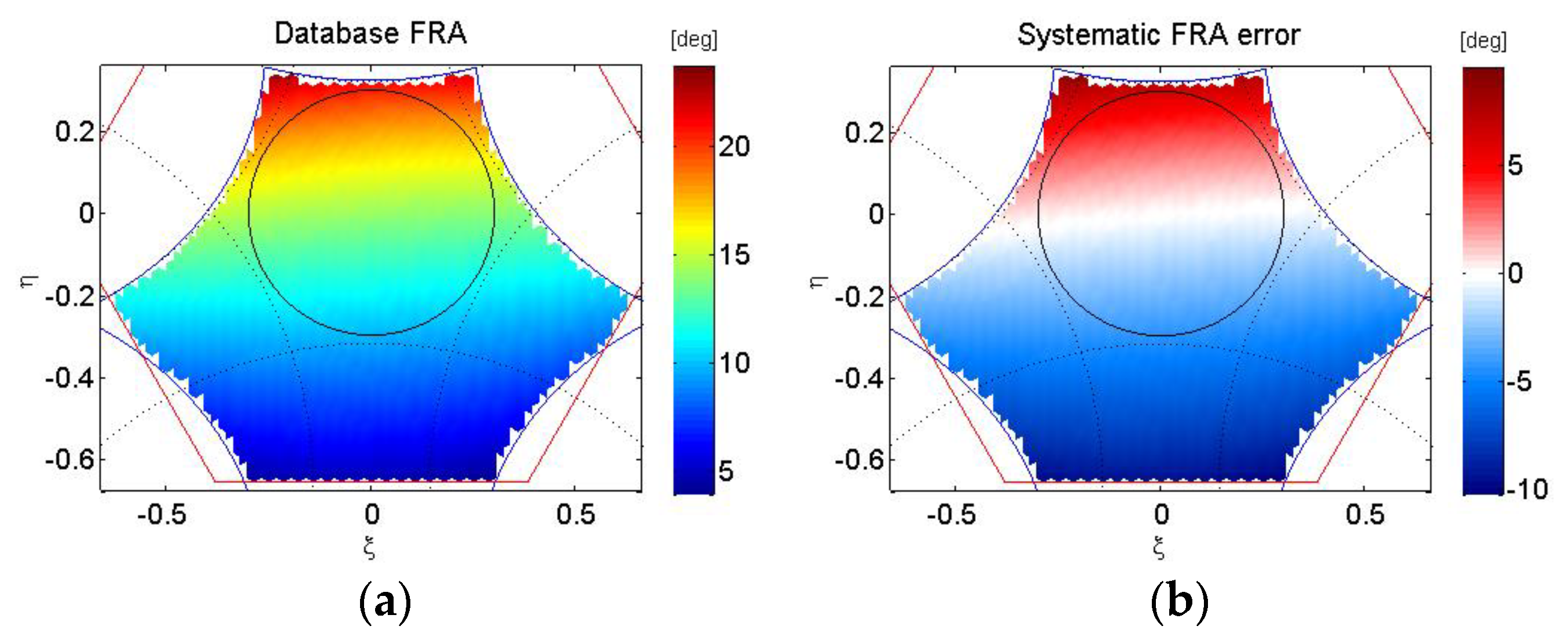
In a previous paper [9], the FRA was estimated from MIRAS data using spatiotemporal filtering techniques. A unique FRA value per snapshot (at boresight) was retrieved by averaging the FRA over a circle of radius 0.3 around the boresight in the − plane, defining and as the director cosines with respect to the X and Y axes, respectively. Even though this methodology reproduces the natural variation of the Faraday rotation accurately, it is not enough to use one FRA value for all the EAF-FoV due to its spatial variation within the snapshot. Figure 1a shows the FRA over the EAF-FoV of one snapshot over a descending orbit in October 2011. The circle of radius 0.3 is drawn in black. The FRA was calculated using Equation (1) and reading the geomagnetic field and the VTEC from the external datasets [14,17], respectively. The error when the boresight FRA is considered for all pixels over the EAF-FoV is shown in Figure 1b.
It is known that the VTEC and therefore the FRA vary with solar activity, which can be assessed using sunspot numbers [18], and in a geographical and temporal way [7,19]. SMOS data is here considered within the 24th sun cycle, which started on January 4th, 2008, with each cycle lasting about 11 years. The sun’s peak activity during this cycle was reached on March 2014 [18,19]. It is also important to note that the value of the FRA reaches its highest point during the year in the March equinox due to the sun’s illumination geometry over the earth during that season.
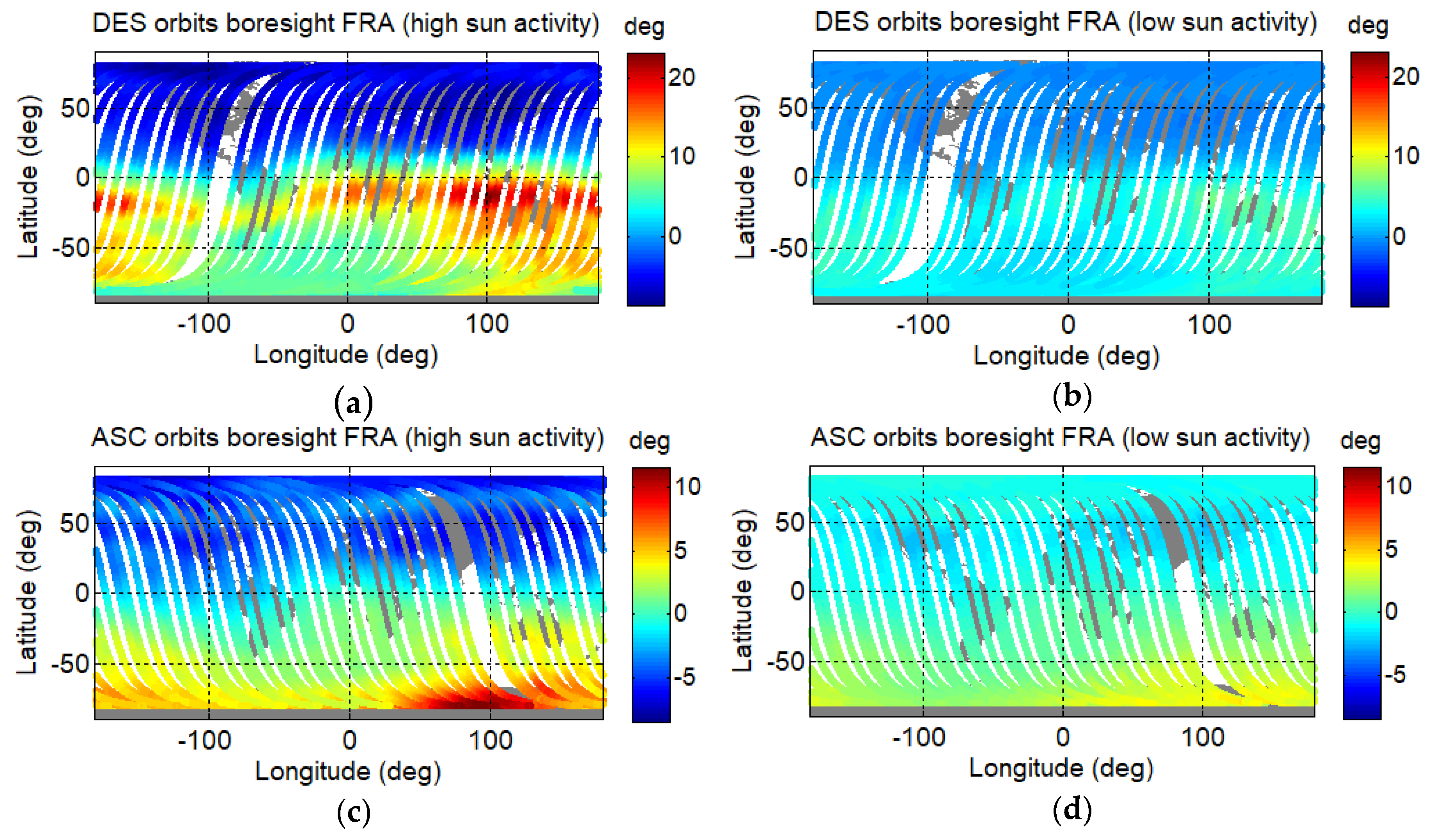
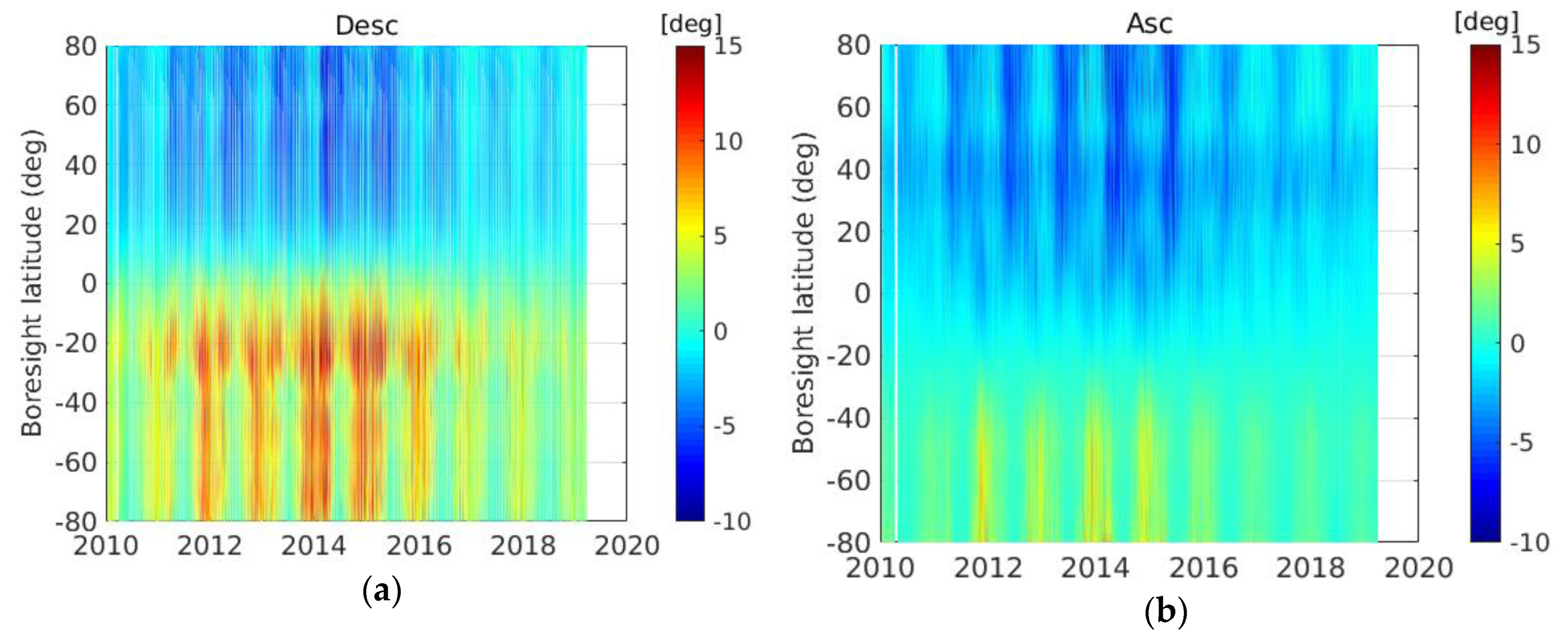
The geographical variability of the FRA is presented in Figure 2. Equation (1) and the same mentioned external databases were used again to calculate the FRA at the coordinates of the SMOS boresight over a 3-day period. Two different time frames were used: one with high FRA (March 19th to 21st, 2014) and another with low FRA (January 14th to 16th, 2011). The FRA of both descending (DES) and ascending (ASC) orbits are shown for each period (be aware of the different scales in ASC/DES maps). Additionally, the latitude-time Hovmöller plots of the FRA for the entire mission are shown in Figure 3 for descending and ascending orbits to show the FRA temporal variability. The FRA was calculated over the eastern Pacific Ocean using also the database VTEC. These Hovmöller diagrams confirm the selected periods of high and low FRA.
From these figures, it is perceived that descending orbits present much higher FRA and higher dynamic ranges than ascending ones. In the afternoon local time, the surviving amount of VTEC generated by sunlight during the preceding hours is higher than in the morning local time [19] and because SMOS is in a 6 am—6 pm sun-synchronous orbit, the resulting FRA range is large. Consequently, in the first stage, the analysis was focused on descending orbits. A preliminary analysis was done during the March equinox of 2011 [20], but it was later decided to extend the study to the March equinox of 2014 as well, because, as can be perceived in Figure 3, the highest peak of FRA in the SMOS mission up until now corresponds to that period of time.
2.2. Data Sources
2.2.1. SMOS Brightness Temperatures
MIRAS measures the brightness temperature of each scene providing a full-polarimetric block (Tx, Ty, and Txy) every 2.4 s [16]. The MIRAS Testing Software (MTS), developed by the Polytechnic University of Catalonia (UPC), is an independent processor used as a breadboard to test calibration and image reconstruction algorithms before their introduction into the SMOS Level 1 operational processor [21]. The SMOS brightness temperatures used in this work were processed by MTS from level 0 (raw data) up to level 1C (geolocated brightness temperatures).
2.2.2. Geomagnetic Field and the Consolidated VTEC Databases
The directly proportional relationship between the FRA and the VTEC is determined by Earth’s electromagnetic field. Thus, a geomagnetic field dataset is needed. This dataset corresponds to the 12th Generation International Geomagnetic Reference Field (IGRF) [13], which is calculated by the International Association of Geomagnetism and Aeronomy (IAGA). It can be found in [17] and it has a geographical resolution of 5° in longitude and 2.5° in latitude for the entire globe as well as a daily temporal resolution.
SMOS level 1 data includes the consolidated VTEC. It is built by the SMOS Data Processing Ground Segment (DPGS) [14], and it can be obtained in the SMOS dissemination service website [15]. The data also has a geographical resolution of 5° in longitude and 2.5° in latitude for the entire globe but a temporal resolution of 2 h.
2.2.3. SMOS Level 2 VTEC (DTBXY Product)
The SMOS level 2 processor computes the VTEC with a methodology that uses the third Stokes parameter and an external database of VTEC. The VTEC value is calculated for the zone of the snapshot with highest sensitivity of TB to VTEC, which corresponds to pixels in the area around , (, . Then, that value is used for the entire EAF-FoV. This VTEC is called A3TEC [11].
2.2.4. GPS VTEC
This third VTEC source consists on VTEC maps with a temporal resolution of 2 hours and a geographical resolution of 5° in longitude and 2.5° in latitude calculated from daily sets of GPS differential code bias values [23]. The IGS Ionosphere Working Group (Iono-WG) calculates the VTEC, which is named IGS Global Total Electron Content (IGSTEC). It is stored in IONEX format, and it can be downloaded from the official server (CDDISA at GSFC/NASA).
2.3. FRA End-to-End Simulator
In order to evaluate different approaches to retrieve VTEC maps, a first version of a FRA simulator was presented in [10]. This simulator was refined until it worked properly for the assessment. The improved FRA simulator is explained in this section.
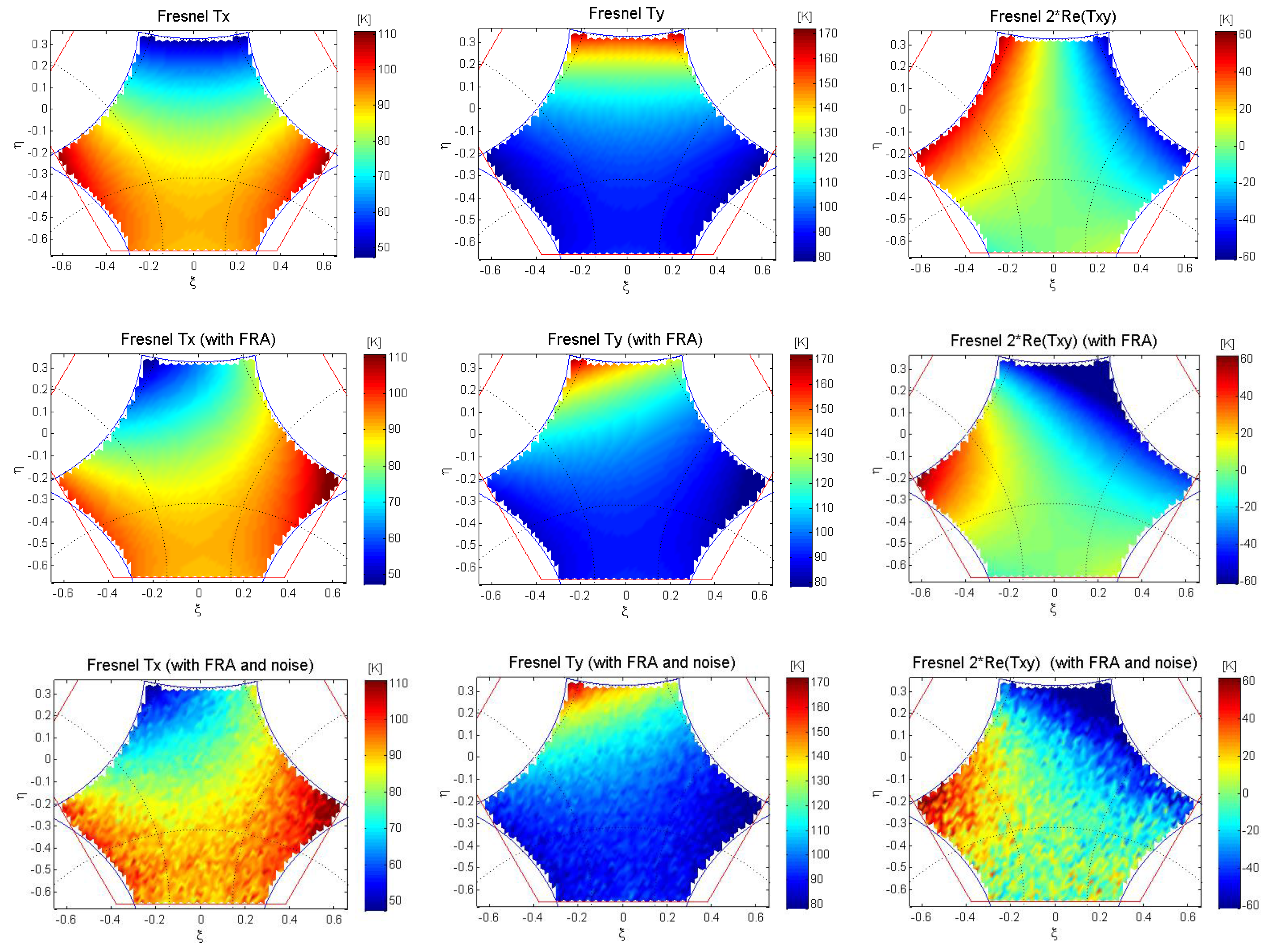
For each snapshot, the and coordinates defined in the antenna frame (director cosine plane) are translated to Earth’s surface coordinates. The incidence angle and the geometric rotation angle are computed using standard geometry [16]. Then, a simple geophysical model is used to simulate the Earth’s emissions. Ocean TB are built by assuming a Fresnel model with a typical salinity value of 35 psu and a typical sea surface temperature of 294 K. Open ocean TB images per polarization, assuming a uniform ocean, are shown in the top row of Figure 4 (left: X-pol, middle: Y-pol, right: third Stokes parameter).
To add the Faraday rotation for each pixel, Equation (1) is used together with both the VTEC and the geomagnetic databases. This Faraday rotation angle derived from external datasets shall be referred to as “database FRA” from now on in this paper. Once calculated, it is added to the geometrical angle to obtain the total rotation per pixel when simulating Earth’s emissions. Open ocean TB images taking into account the FRA are shown in Figure 4 (middle row).
Then, the effect of measurement noise is included in the simulator. To do so, first the radiometric sensitivity per polarization is calculated. The radiometric sensitivity corresponds to the smallest radiometric temperature that the instrument can detect. It is defined in the antenna reference frame as follows [24]:
where corresponds to the elementary area in the () grid defined by ; refers to the distance between antennas normalized to the wavelength (d = 0.875 in SMOS); corresponds to the addition of the average antenna temperature () and the average receiver noise temperature at the antenna plane (), both being different per polarization (see typical values for the open ocean in Table 1); is the receiver noise equivalent bandwidth that in MIRAS equals 19 MHz; is the effective finite integration time (, where corresponds to the integration time that is 1.2 s for pure X and Y epochs and 0.4 s for mixed epochs and for SMOS 1 bit/2 level digital correlator [25]); is the antenna equivalent solid angle that equals 1.4; is the antenna pattern measured on the ground; is the used window factor that in this case is a Blackman window (); and is the total number of visibilities samples that in MIRAS is 2791.
The effect of noise is added to the TB with a normal distribution of zero mean and the standard deviation equal to the radiometric sensitivity of each pixel. Figure 4 (bottom row) shows typical open ocean TB images with FRA, including the effect of noise.
MIRAS measures sequentially for each polarization at different instants in time. When processing, one single instant is used for all polarizations. This introduces an error when translating the brightness temperatures from the polarization (antenna frame) to polarization (ground plane) that is unavoidable in the processing.
VTEC maps can be calculated with the FRA estimated using the TB. These maps can then be used in the correction of the FRA per pixel in the field of view (FoV) of every snapshot of the trace.
2.4. VTEC Retrieval from Radiometric Data
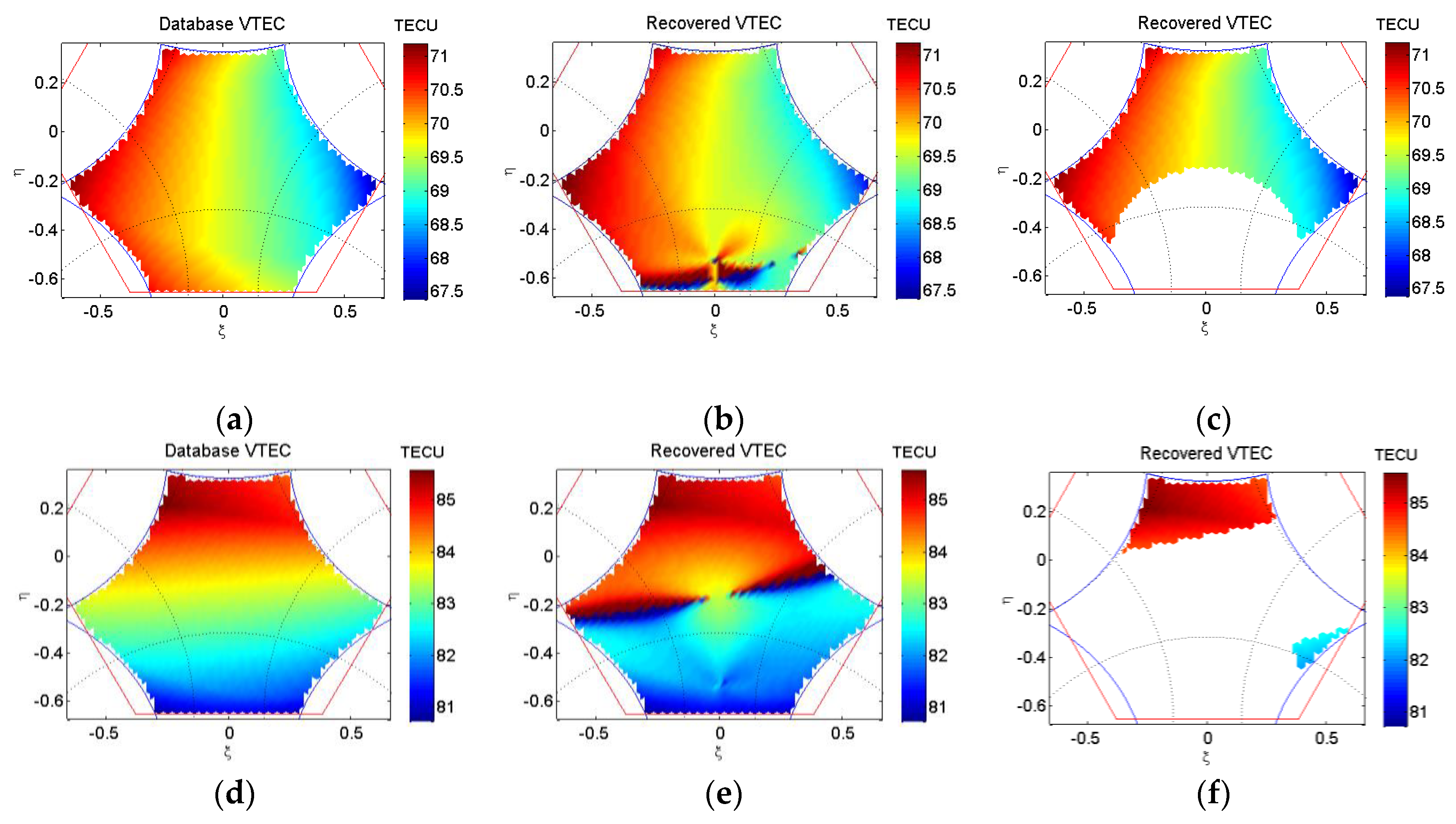
From the brightness temperature snapshots, the FRA can be retrieved by applying Equation (3). An indetermination emerges when both the numerator and the denominator tend to 0 ( and ); that occurs at low incidence angles [26]. To avoid it, pixels with incidence angles lower than 25° are discarded. Figure 5a shows a database VTEC snapshot from a descending SMOS overpass over the Pacific Ocean on March 20th, 2014. Figure 5b shows the retrieved VTEC snapshot where some pixels are affected by the indetermination of Equation (3). Figure 5c shows the retrieval once pixels causing the indetermination of Equation (3) are rejected with the chosen threshold.
Once the FRA is retrieved, the VTEC is calculated using Equation (1). This equation presents an indetermination when the geomagnetic field is orthogonal to the wave propagation direction, which occurs close to the Equator, in a zone where the FRA vanishes. To avoid this indetermination, pixels accomplishing are rejected by using an appropriate threshold established empirically (). Figure 5d shows another database VTEC snapshot from a descending SMOS overpass over the Pacific Ocean on the same date, March 20th, 2014, in order to compare it with its retrieval (Figure 5e). The error introduced by the indetermination is noticeable. Figure 5f shows the retrieval once pixels causing the indetermination of Equation (1) are rejected with the chosen threshold (pixels causing indetermination of Equation (3) were rejected previously). It is important to remark that this threshold is only used when the geomagnetic field is orthogonal to the signal path.
After retrieving VTEC snapshots, the geolocation is done at an altitude of 450 km in an ETOPO5 grid (1/12°).
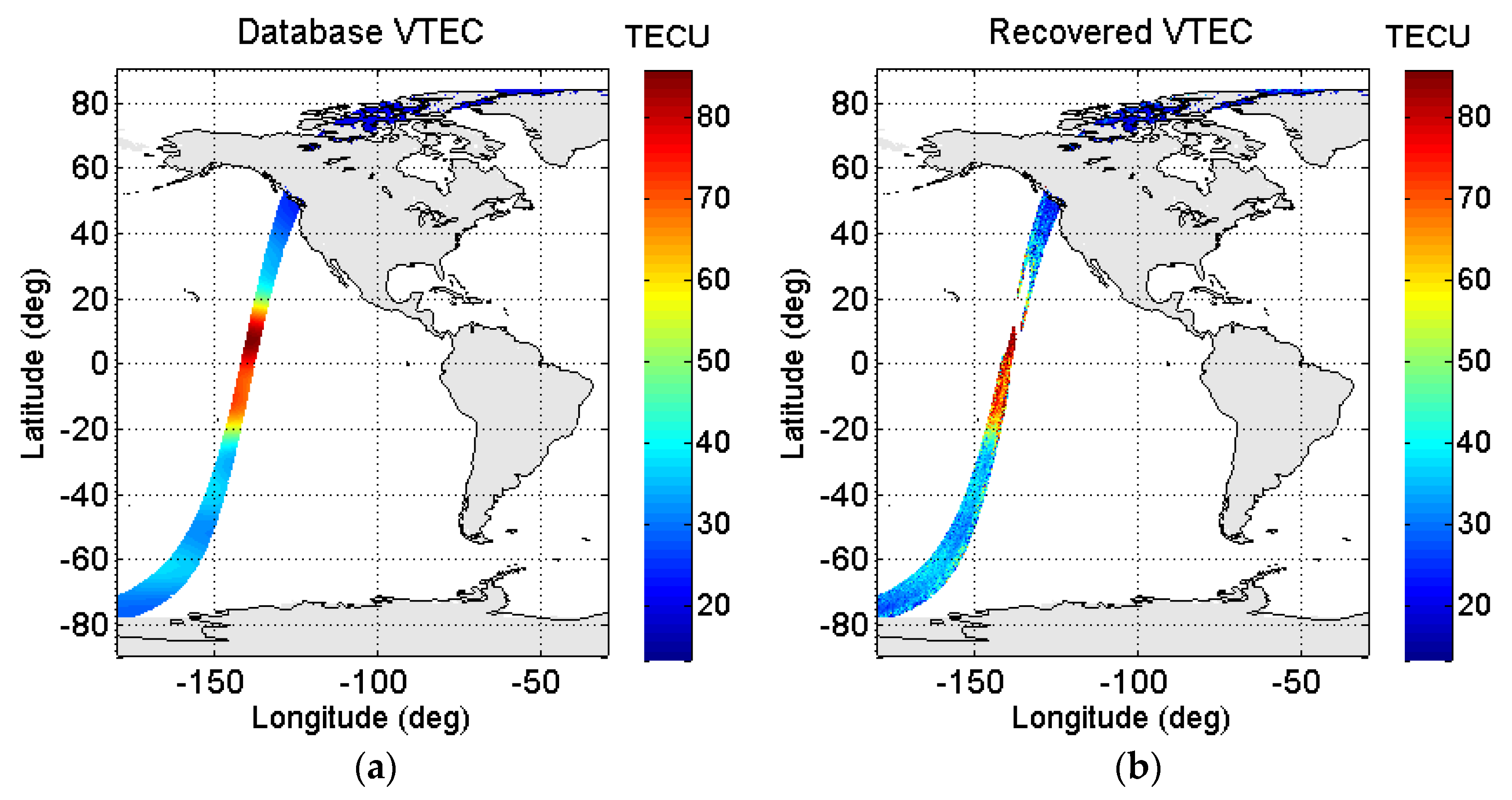
Figure 6 shows the VTEC maps of a descending SMOS overpass in the Pacific Ocean (March 20th, 2014) processed with the simulator (taking into account the effect of the noise). In order to have a reference, the database VTEC can be seen in the left (Figure 6a). Because both the geographical (5° in longitude and 2.5° in latitude) and temporal resolution (2 h) of the “Consolidated TEC” is coarse, a spatiotemporal interpolation is done in order to obtain the VTEC in that SMOS overpass in an ETOPO5 grid. In Figure 6b, the retrieved VTEC is shown, where it is noticeable how the effect of noise introduces errors in the retrieval.
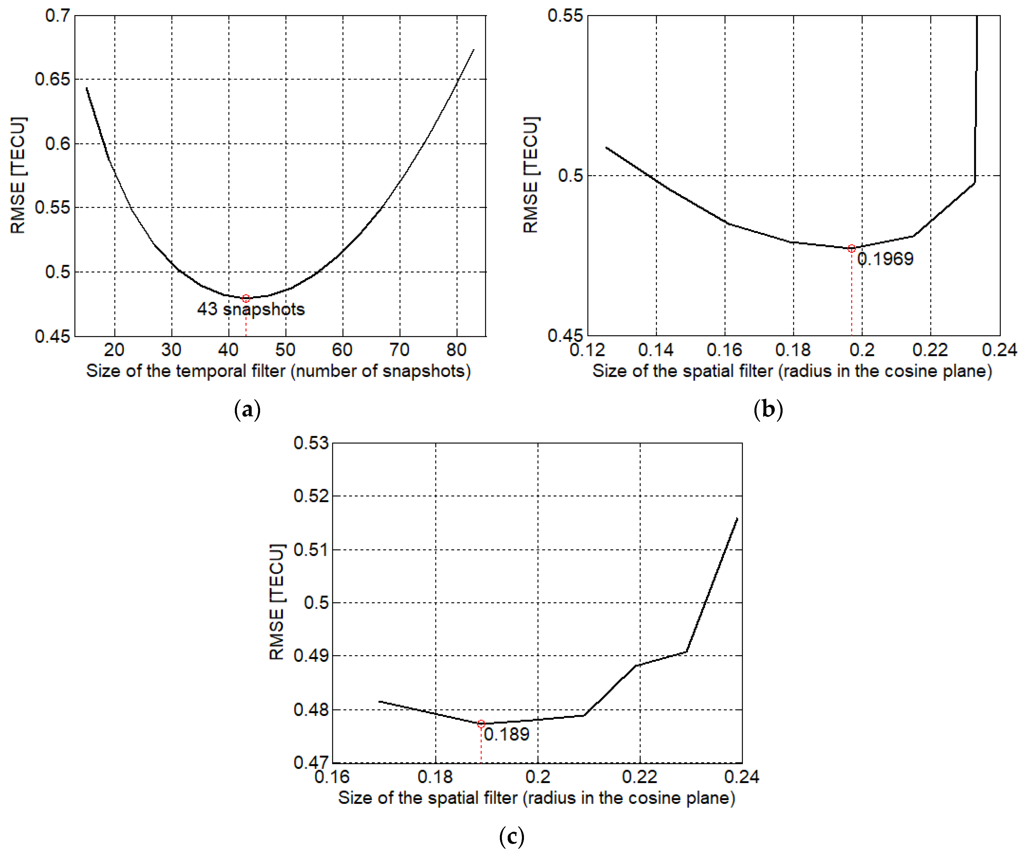
To reduce the effect of noise and artifacts in the retrieved VTEC from SMOS data, spatiotemporal filtering techniques are required [9]. The sizes of both filters were optimized with the simulator that takes into account the effect of noise. To do so, the size of the spatial filter was set to 0.179 in the director cosine plane (10 times the minimum ) in TB snapshots and the length of the temporal filter was varied from 15 to 83 snapshots with a step of 4 snapshots. Figure 7a shows the root mean square error (RMSE) of the deviations with respect to the database VTEC of this optimization. The temporal filter is an averaging triangular window considering the current snapshot with the highest weight. Its size was then fixed to 43 snapshots (optimum value from Figure 7a) and the size of the spatial filter was optimized by varying its radius from 0.1253 to 0.2506 with a step of 0.0179. The RMSE of this optimization is shown in Figure 7b, where it can be seen that the optimum size of the spatial filter corresponds to a radius of 0.1969 in the cosine plane. Finally, a fine tuning was done for the size of both filters to select which ones to use. The optimum temporal filter corresponds to 43 snapshots, again, and the spatial filter to 0.189 in the plane (Figure 7c). It is important to remark that the temporal filter is applied to TB snapshots, and the spatial filter to VTEC snapshots at the antenna frame. The spatial filter was also tested over the ground instead of at the antenna reference frame. To do so, the window size of the spatial filter was calculated to be equivalent to the spatial filter at the antenna, which corresponds to a radius of approximately 190 km over the ground. There was not a clear improvement in the retrieval, but there was an important difference in the execution time, with the calculation over the ground being much slower. Therefore, the spatial filter was applied at the antenna reference frame.
Hence, the methodology consists of:
- Applying a temporal filter as a triangle filter with a window of 43 TB snapshots.
- Computing the FRA from the TB using Equation (3), rejecting pixels with incidence angles lower than 25° in order to avoid the indetermination in pixels with and .
- Computing the VTEC from the retrieved FRA using Equation (1), rejecting pixels with a threshold of to avoid the indetermination that emerges from that equation.
- Applying a spatial filter with a radius of 0.189 in the director cosine plane of VTEC snapshots.
- Generating VTEC maps in an ETOPO5 grid at 450 km of altitude.
2.5. Recovered VTEC Maps with Simulated Data
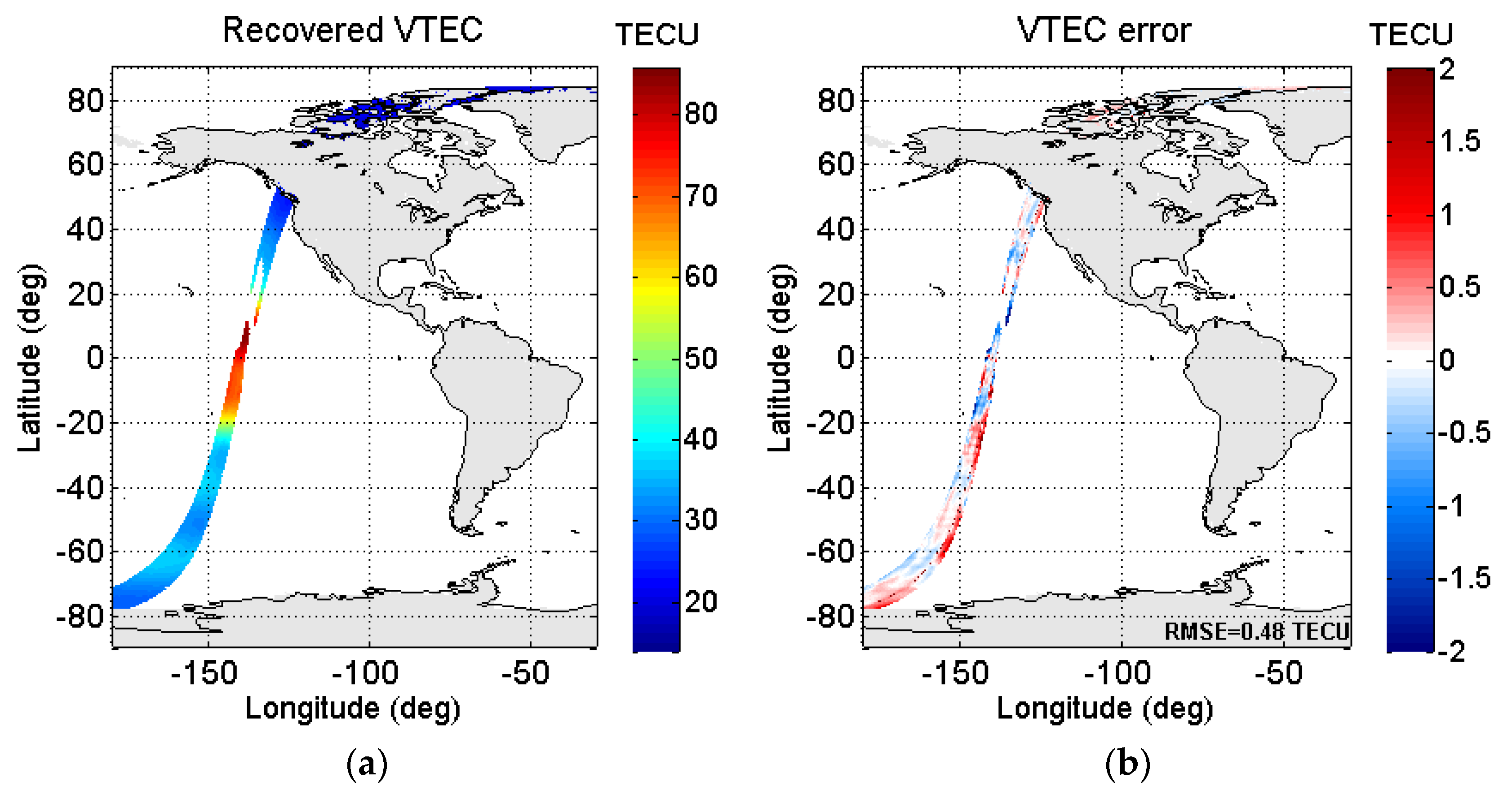
The descending SMOS overpass in the Pacific Ocean on March 20th, 2014 was processed in the simulator using the methodology described and the results are shown in Figure 8. The recovered VTEC is shown at the left and the error of the retrieval with respect to the database is shown at the right. The retrieved VTEC follows the variation of the database VTEC with a RMSE of 0.48 TEC units. It can be seen that the error in the retrieval does not follow any systematic pattern. The highest error is found close to where the geomagnetic field is orthogonal to the wave propagation direction (indetermination in Equation (1)).
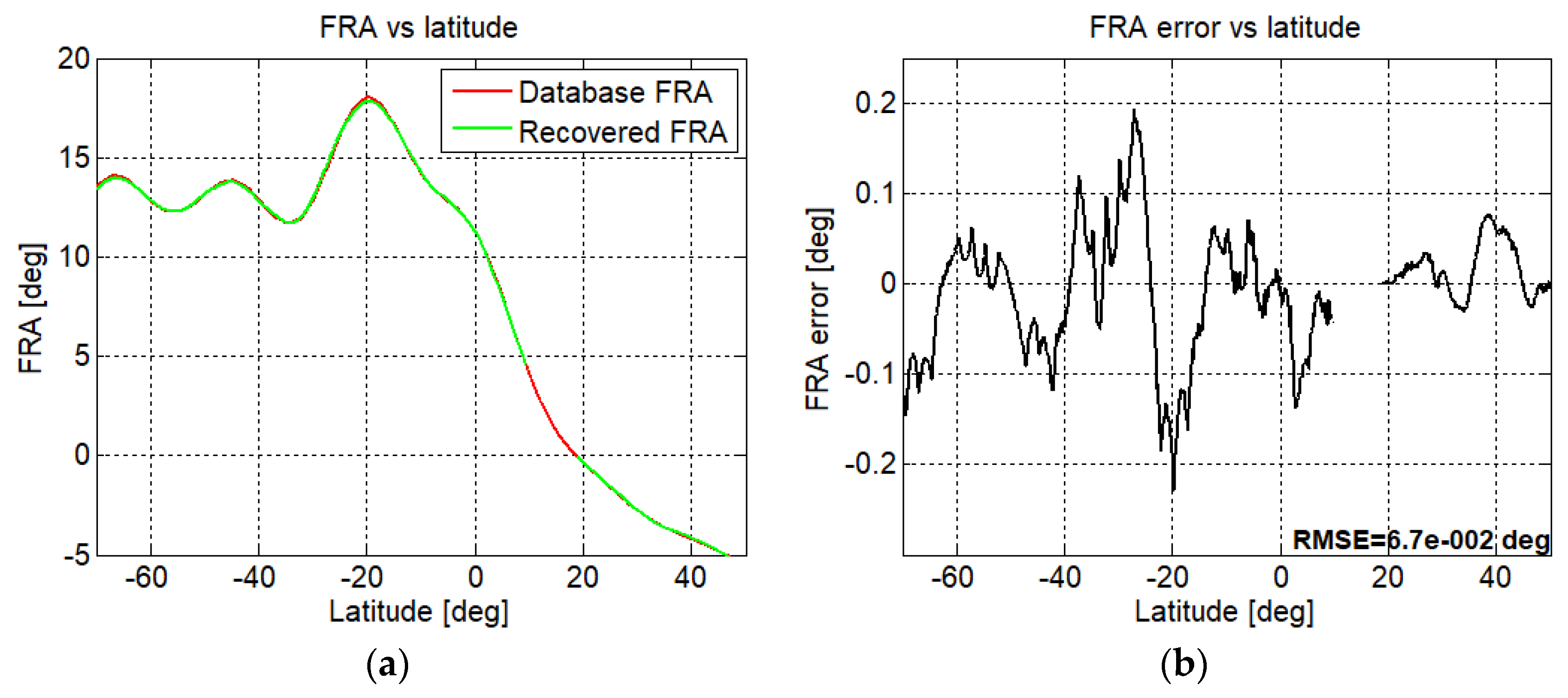
By applying Equation (1) with the database VTEC, an FRA reference can be obtained. Likewise, the FRA can be computed from the retrieved VTEC for all the pixels in the EAF-FoV. Figure 9 shows the database FRA (red) and the simulated retrieved FRA (green) as a function of latitude of a pixel with and , as well as the error of the FRA retrieval with respect to the database FRA. The gap in the retrieval comes from the rejected pixels in the zone of the orthogonality that is between the geomagnetic field and the wave propagation direction (incidence angle), where it can be seen how the FRA vanishes.
The methodology is able to recover the FRA following the geophysical and temporal variation with a negligible error (with a RMSE of 0.07°), showing good performance.
3. Results and Discussion
Considering the promising results obtained when assessing the methodology with the simulated data, SMOS radiometric data were processed to derive VTEC maps.
3.1. VTEC Retrievals from SMOS Data
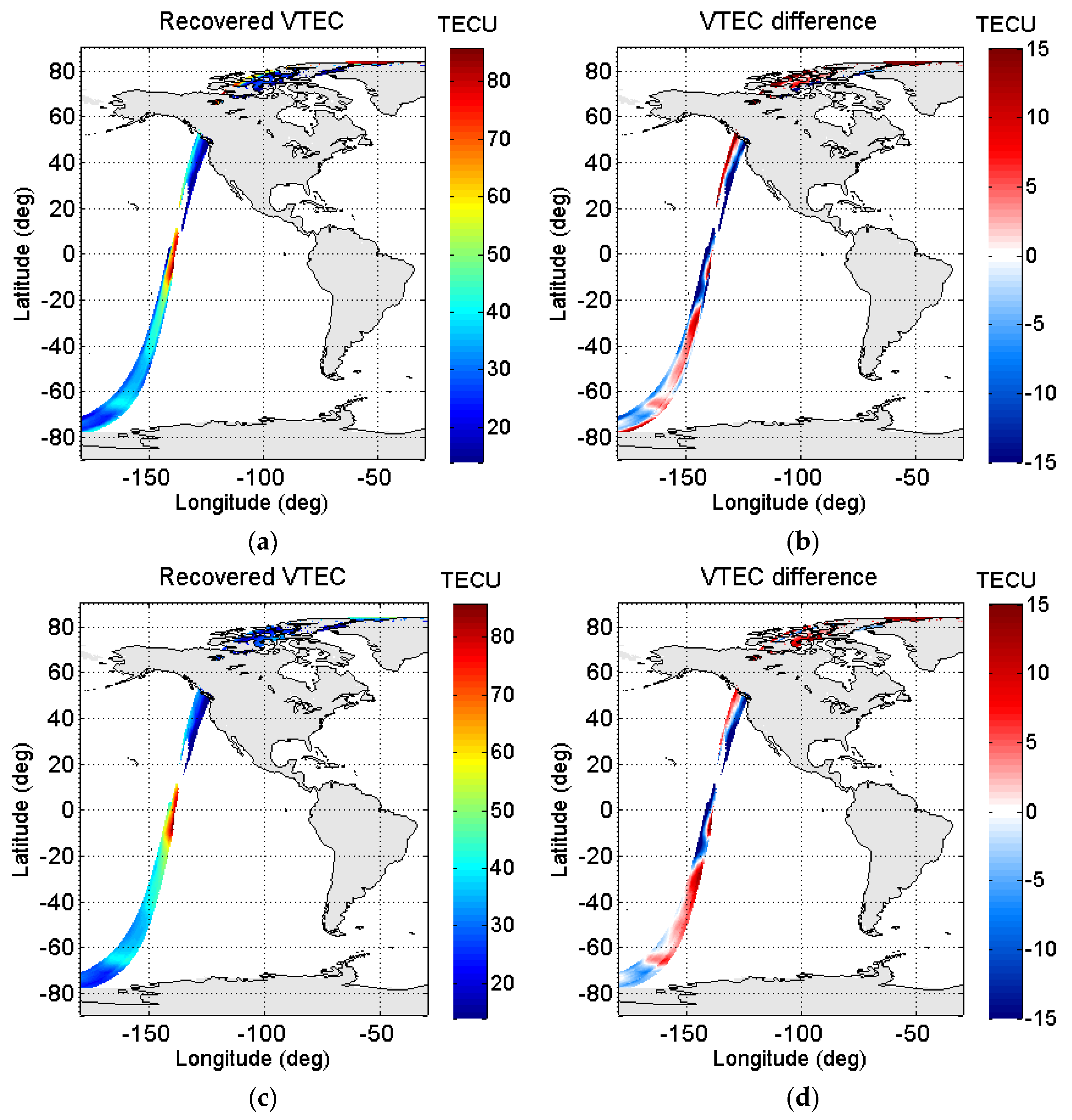
Results of the retrieved VTEC with SMOS radiometric data, and the difference between the retrieved VTEC and the database VTEC (used here as a reference) are shown in Figure 10 (top). The recovered VTEC presents a systematic pattern with higher differences in the edges of the swath. This pattern did not appear in the retrieved VTEC from simulated TB. It needs to be characterized at some point in future research.
In order to mitigate the effect on the swath laterals, some empirical approaches were assessed. The first approach used only the alias free-field of view (AF-FoV) instead of using the EAF-FoV region. By doing so, the retrieval of FRA could only be performed over a much narrower swath after a complete SMOS overpass. Hence, a second attempt was based on assigning the average VTEC of the AF-FoV to the entire EAF-FoV in each snapshot [9], disregarding the TEC variability along the snapshot. The third and selected approach consists of extending the value of the VTEC in the pixels of the AF-FoV closest to the EAF-FoV to the latter. The processed orbit using that approach and its difference with respect to the database VTEC are shown in Figure 10 (bottom).
The lateral bands of the southern hemisphere become softened. In the northern hemisphere, a similar softening happens, though not as noticeably as in the southern hemisphere. Additionally, the retrieved VTEC is generally lower than the database VTEC, something that in the simulation does not happen. Table 2 shows the root mean square of the difference (RMSD) between the retrieved and the database VTEC in the EAF-FoV and the difference between the retrieved VTEC in the AF-FoV extended to the EAF-FoV with respect to the database VTEC. For a reference, the statistics of the simulated retrieval are also presented. The statistics are calculated in a range of latitudes between 60° N and 60° S.
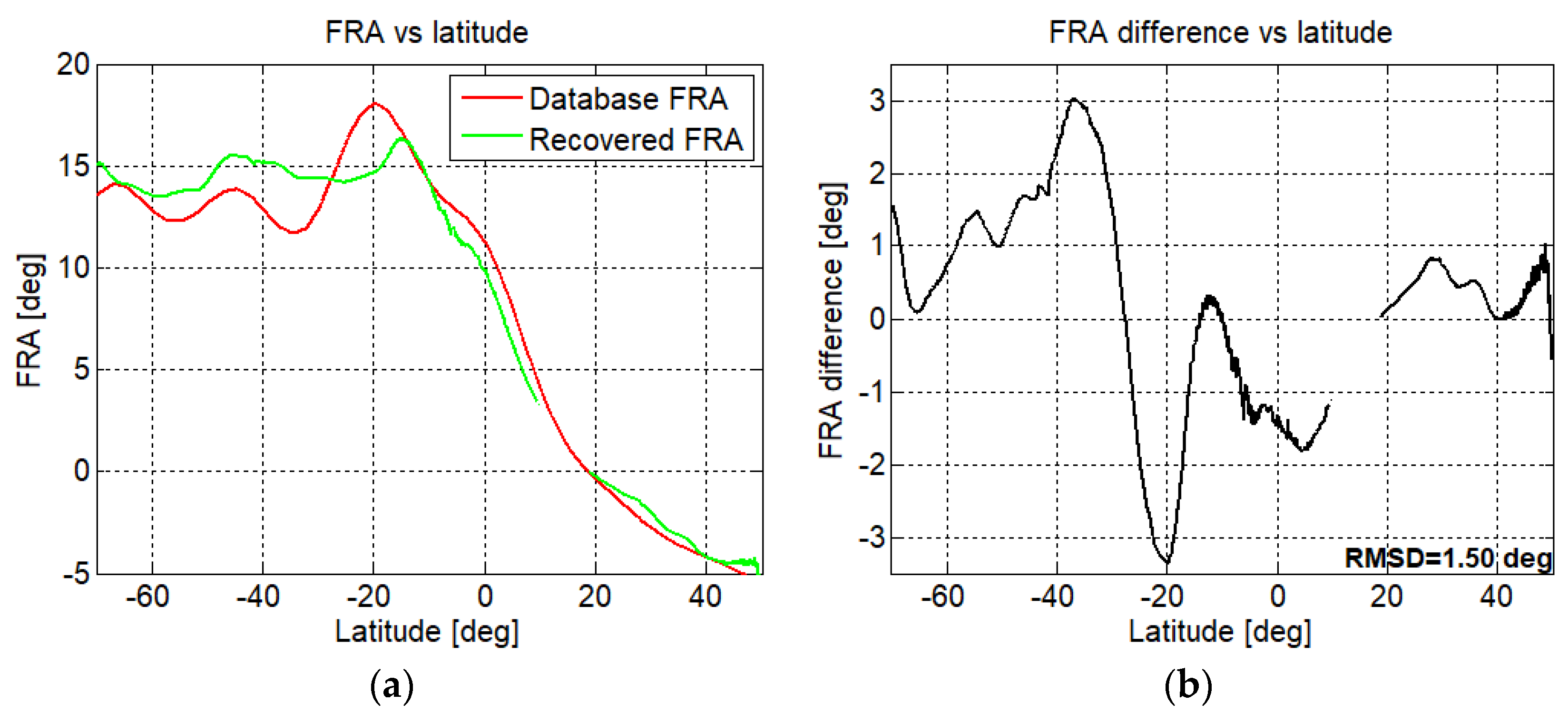
Figure 11 shows the retrieved FRA (from the VTEC shown in Figure 10c) as a function of the latitude. The database FRA (red) is compared against the retrieved FRA (green) at a pixel in the center of the swath ( and ) and its difference is shown in Figure 11b. When processing SMOS radiometric data with the proposed methodology, even though it is possible to recover the FRA geophysical and temporal variation, there is a difference with respect to the database FRA.
Greater differences are perceived in the southern hemisphere. In the northern hemisphere and up to 10° S, both FRAs are very similar, a scenario that does not happen when analyzing pixels in the laterals of the overpass (not shown). This is noticeable in Figure 10d. Still, the root mean square of the difference between the retrieved FRA and the FRA database (Figure 11b) is 1.5°, which represents only 6.50% of the dynamic range of the database FRA.
3.2. Comparison of Retrieved VTEC from SMOS with Other External VTEC Sources
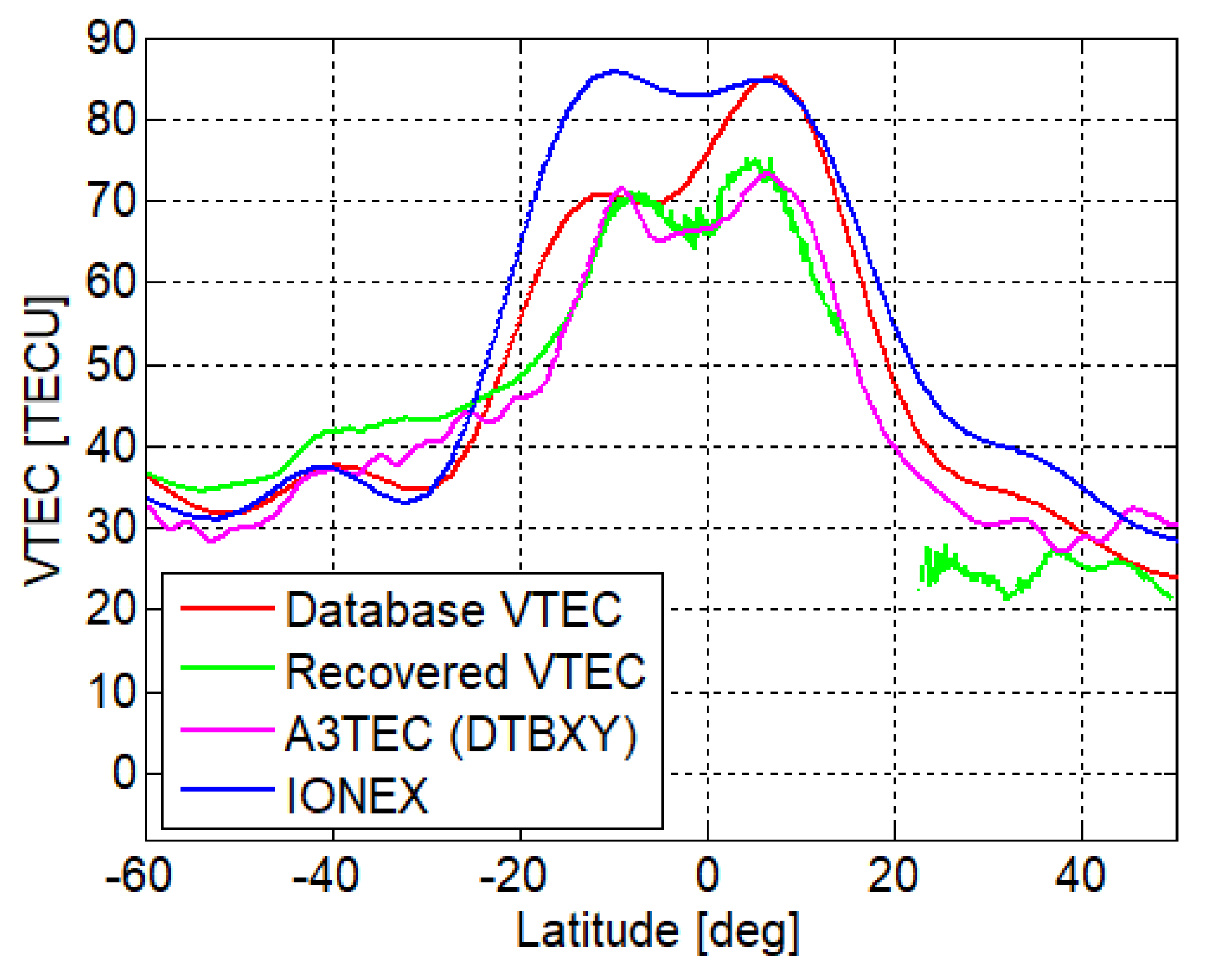
In this section, a comparison of the VTEC retrieved with the proposed methodology and that from other sources shown in Section 2 is presented in Figure 12 shows the VTEC of the middle pixel of the swath as a function of the latitude provided by different sources. The line in red corresponds to the database VTEC, the green line to the recovered VTEC using the proposed methodology, the magenta line to the A3TEC (VTEC from the DTBXY product), and the blue line to the IONEX VTEC coming from GPS data [23].
The retrieval with the proposed methodology (green line) follows the temporal-geophysical variation that the A3TEC (magenta) presents. Both of them come from SMOS radiometric data. The gap around 20° N corresponds to the zone where the geomagnetic field is orthogonal to the wave propagation direction causing the Faraday rotation to vanish. The A3TEC provides data in that zone but tends to the value of the database VTEC, which is expected, because in the procedure to retrieve it, that auxiliary database is used as a first guess, and in that zone, the sensitivity of the TB to TEC is very low. The retrieved VTEC with the proposed methodology has fewer ripples than the A3TEC. It was found that the origin of those ripples is due to the remaining noise as reported in [11]. IONEX is always above the VTEC value retrieved from SMOS data, both using the methodology proposed in this paper and the VTEC from DTBXY products, which is in agreement to [11]. The presented methodology proposes an alternative to the current methodology used in order to eliminate the dependency on any external database VTEC.
3.3. Impact of RFI Contamination in the Retrieved VTEC
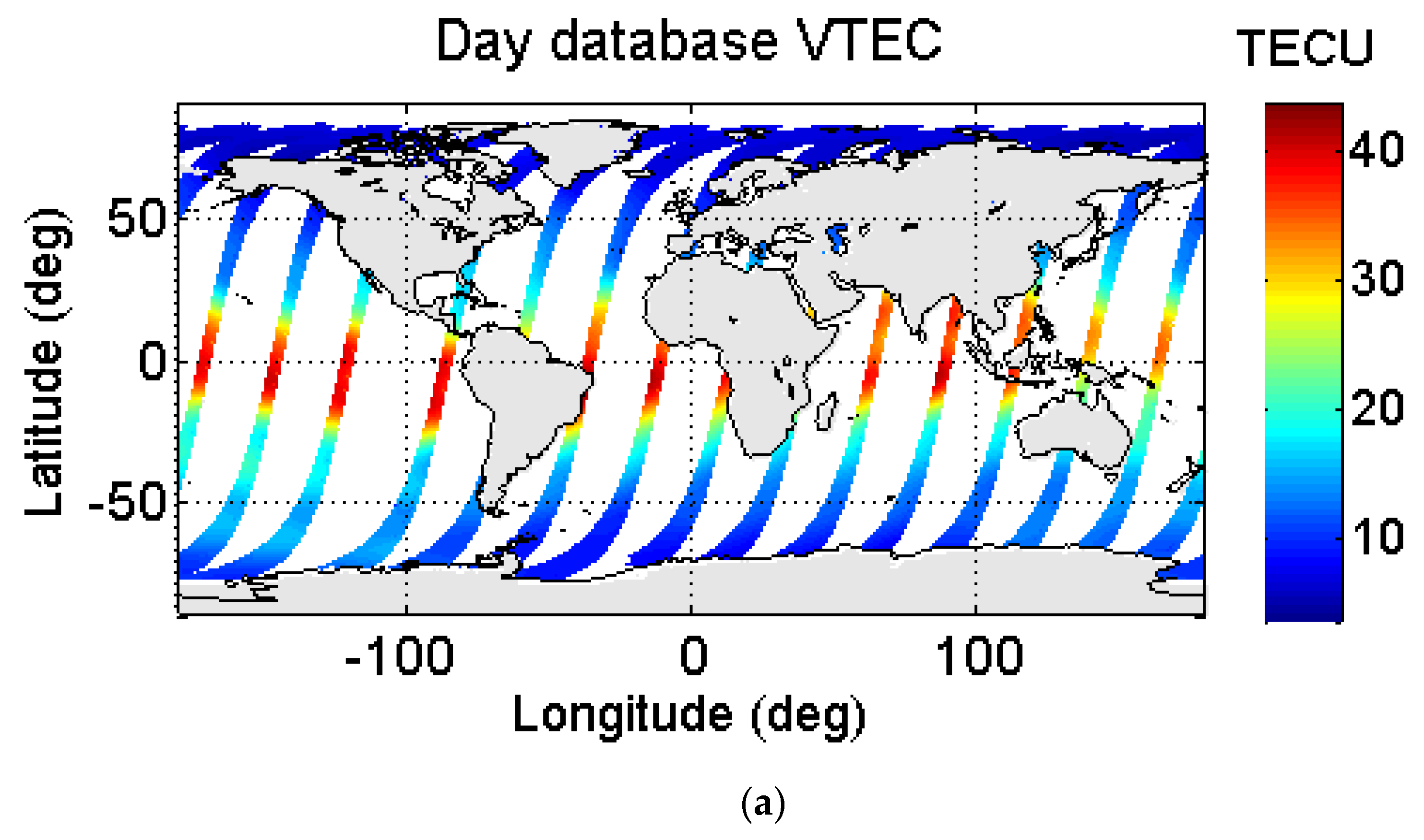
In order to analyze the performance of the proposed methodology on a global scale, the analysis was extended to all the descending orbits over the ocean on March 21st, 2011. This particular year was chosen because it opened up the possibility to evaluate the impact in the presence of radio-frequency interference (RFI). The RFI contaminates the TB, which has an impact in the recovered VTEC. The retrieved VTEC with the proposed methodology and the one provided by the database VTEC (used as a reference) are shown in Figure 13 as well as the difference between them.
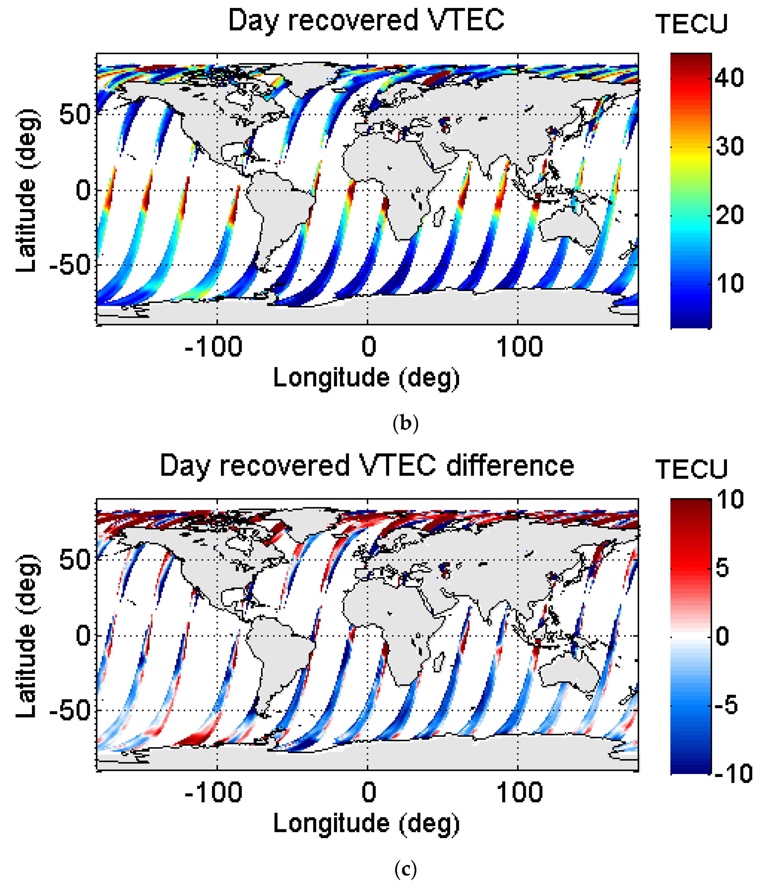
Greater differences between the recovered and the database VTEC are concentrated at northern, high latitudes, close to ice edges. There were significant differences over the Bering, the Beaufort, and the Barents Seas on that date (see zoomed in portions of Figure 14a,c, respectively). We analyzed whether this was related to TB contamination by RFIs (radio-frequency interferences) sources. In 2011, there were RFIs affecting the Bering Sea, which were switched off in 2012 [27]. The VTEC retrieval of a descending orbit over the same region on March 20th, 2012 was processed and it is shown in Figure 14b. When the RFI was shut down, it was possible to recover a VTEC that was less affected by errors. Similarly, a descending orbit over the Barents Sea on March 22nd, 2019 was processed (when the RFI source was already switched off) and it is shown in Figure 14c. Once again, it was confirmed that RFIs were affecting the VTEC retrieval in 2011 (Figure 14c).
4. Conclusions
Measuring the Faraday rotation from radiometric data allows for the estimation of the total electron content of the ionosphere by using an inversion procedure. This allows for the possibility of creating a VTEC product from SMOS data. Eventually, this product can then be re-ingested in the SMOS level 2 processor in order to improve the geophysical retrievals.
The proposed methodology works independently of the target seen by the instrument. This is an important improvement with respect to the current methodology that also derives VTEC maps from SMOS radiometric data [11], which use a forward radiative model and are focused only over the ocean because SMOS’s main purpose is to improve salinity measurements. Moreover, the developed methodology estimates the VTEC for all the pixels in the EAF-FoV with information from different incidence angles, instead of using only the FoV region with the highest sensitivity to TEC, and extending this value across the FoV as does the methodology detailed in [8].
The analysis of the retrieved VTEC maps has been focused over the ocean, where the impact of ionospheric corrections is stronger. These maps have been inter-compared with the database VTEC, the IONEX GPS data, and the A3TEC products. The retrieved VTEC maps provide values generally lower than those of the external VTEC database and the IONEX GPS data, which is in agreement with the differences found when comparing the other SMOS-derived product (A3TEC) with the same two external data sources [8]. However, SMOS-derived VTEC products cannot be fully validated by comparing them with the external VTEC database and the IONEX GPS data, since the spatial resolution of the latter ones is much coarser than that provided by the SMOS products. The comparison between both SMOS-derived VTEC products reveals greater differences in the northern hemisphere. The origin of these discrepancies needs to be investigated.
Further work is needed to evaluate the feasibility of providing global SMOS-derived VTEC maps, including ocean, land, and ice. The main challenge is to obtain accurate TEC retrievals over land areas in (i) regions where SMOS TB measurements are degraded by strong RFI contamination and (ii) regions where TB at horizontal and vertical polarizations are very similar (such as in dense forests), making the TEC retrieval ill-conditioned. A dedicated study of retrieved VTEC over land to assess the performance of the proposed method on a global scale is currently on-going. Besides, the Faraday rotation vanishes in regions of the earth where the geomagnetic field is orthogonal with the signal path. Therefore, the retrieval of VTEC in these regions is not possible and maps will present data gaps. Improvements over the ocean also need to be addressed. The retrieved VTEC maps present a remaining systematic pattern (more noticeable in the northern hemisphere, as shown in Figure 14c) that might be introduced by the instrument when measuring the Faraday rotation (not present in the simulation experiments). Ongoing work is focused on characterizing this FRA systematic pattern in a region and for a period with very low FRA values, so the measurement can be assumed as a systematic error of the instrument, and a correction can be built upon that.
The recovered VTEC maps could be used in the SMOS Level-2 processor to correct the Faraday rotation, which could potentially improve geophysical retrievals, as reported when using the A3TEC method [11]. As a preceding step to analyze the impact of using these VTEC maps on salinity retrievals, the computation of the OTT (ocean target transformation) will be evaluated and used in order to correct the spatial bias presented in the TB as is done by the SMOS ocean salinity team [28]. If an improvement in the stability of the OTT is achieved, more accurate salinity retrievals by using these VTEC maps would be expected.
Author Contributions
Conceptualization, F.T., Investigation, R.R., N.D., V.G.-G., and I.C., methodology, R.R., N.D., V.G.-G., I.C., and I.D., supervision, N.D., V.G.-G., and I.C., writing—original draft, R.R., writing—review an editing, N.D., V.G.-G., I.G., and M.M.-N. All authors have read and agreed to the published version of the manuscript.
Funding
This research was supported by the European Space Agency and Deimos Engenharia (Portugal), SMOS P7 Subcontract DME CP12 no. 2015-005; ERDF (European Regional Development Fund); by the Spanish public funds, projects TEC2017-88850-R and ESP2015-67549-C3-1-R; and through the award “Unidad de Excelencia María de Maeztu” MDM-2016-0600, financed by the “Agencia Estatal de Investigación” (Spain) and by the European Regional Development Fund (ERDF).
Conflicts of Interest
The authors declare no conflict of interest.
References
- Esa Earth’s Water Cycle. Available online: https://www.esa.int/Our_Activities/Observing_the_Earth/SMOS/Earth_s_water_cycle (accessed on 14 February 2019).
- Kerr, Y.H.; Waldteufel, P.; Wigneron, J.-P.; Delwart, S.; Cabot, F.; Boutin, J.; Escorihuela, M.-J.; Font, J.; Reul, N.; Gruhier, C.; et al. The SMOS Mission: New Tool for Monitoring Key Elements ofthe Global Water Cycle. Proc. IEEE 2010, 98, 666–687. [Google Scholar] [CrossRef] [Green Version]
- Font, J.; Camps, A.; Borges, A.; Martín-Neira, M.; Boutin, J.; Reul, N.; Kerr, Y.H.; Hahne, A.; Mecklenburg, S. SMOS: The Challenging Sea Surface Salinity Measurement From Space. Proc. IEEE 2010, 98, 649–665. [Google Scholar] [CrossRef] [Green Version]
- McMullan, K.D.; Brown, M.A.; Martin-Neira, M.; Rits, W.; Ekholm, S.; Marti, J.; Lemanczyk, J. SMOS: The Payload. IEEE Trans. Geosci. Remote Sens. 2008, 46, 594–605. [Google Scholar] [CrossRef]
- Martín-Neira, M.; Oliva, R.; Corbella, I.; Torres, F.; Duffo, N.; Durán, I.; Kainulainen, J.; Closa, J.; Zurita, A.; Cabot, F.; et al. SMOS instrument performance and calibration after six years in orbit. Remote Sens. Environ. 2016, 180, 19–39. [Google Scholar] [CrossRef]
- Wu, L.; Torres, F.; Corbella, I.; Duffo, N.; Duran, I.; Vall-llossera, M.; Camps, A.; Delwart, S.; Martin-Neira, M. Radiometric Performance of SMOS Full Polarimetric Imaging. IEEE Geosci. Remote Sens. Lett. 2013, 10, 1454–1458. [Google Scholar] [CrossRef]
- Le Vine, D.M.; Abraham, S. The effect of the ionosphere on remote sensing of sea surface salinity from space: Absorption and emission at L band. IEEE Trans. Geosci. Remote Sens. 2002, 40, 771–782. [Google Scholar] [CrossRef] [Green Version]
- Corbella, I.; Torres, F.; Wu, L.; Duffo, N.; Duran, I.; Martin-Neira, M. Spatial biases analysis and mitigation methods in SMOS images. In Proceedings of the 2013 IEEE International Geoscience and Remote Sensing Symposium—IGARSS, Melbourne, Australia, 21–26 July 2013; pp. 3415–3418. [Google Scholar]
- Corbella, I.; Wu, L.; Torres, F.; Duffo, N.; Martin-Neira, M. Faraday Rotation Retrieval Using SMOS Radiometric Data. IEEE Geosci. Remote Sens. Lett. 2015, 12, 458–461. [Google Scholar] [CrossRef] [Green Version]
- Rubino, R.; Torres, F.; Duffo, N.; Gonzalez-Gambau, V.; Corbella, I.; Martin-Neira, M. Direct Faraday rotation angle retrieval in SMOS field of view. In Proceedings of the 2017 IEEE International Geoscience and Remote Sensing Symposium (IGARSS), Fort Worth, TX, USA, 23–28 July 2017; pp. 697–698. [Google Scholar]
- Vergely, J.-L.; Waldteufel, P.; Boutin, J.; Yin, X.; Spurgeon, P.; Delwart, S. New total electron content retrieval improves SMOS sea surface salinity. J. Geophys. Res. Oceans 2014, 119, 7295–7307. [Google Scholar] [CrossRef]
- Yueh, S.H. Estimates of Faraday rotation with passive microwave polarimetry for microwave remote sensing of Earth surfaces. IEEE Trans. Geosci. Remote Sens. 2000, 38, 2434–2438. [Google Scholar] [CrossRef]
- Alken, P.; Maus, S.; Chulliat, A.; Manoj, C. NOAA/NGDC candidate models for the 12th Generation International Geomagnetic Reference Field. Earth Planets Space 2015 2015, 67. [Google Scholar] [CrossRef] [Green Version]
- Barbosa, J. SMOS Level 1 and Auxiliary Data Products Specifications; Indra Sistemas: Alcobendas, Spain, 2014. [Google Scholar]
- ESA SMOS Online Dissemination. Available online: https://smos-diss.eo.esa.int/oads/access/ (accessed on 22 February 2019).
- Martin-Neira, M.; Ribo, S.; Martin-Polegre, A.J. Polarimetric mode of MIRAS. IEEE Trans. Geosci. Remote Sens. 2002, 40, 1755–1768. [Google Scholar] [CrossRef]
- IAGA V-MOD Geomagnetic Field Modeling: International Geomagnetic Reference Field IGRF-12. Available online: https://www.ngdc.noaa.gov/IAGA/vmod/igrf.html (accessed on 22 February 2019).
- Daily and Monthly Sunspot Number (Last 13 Years) | SILSO. Available online: http://www.sidc.be/silso/dayssnplot (accessed on 13 March 2019).
- Kakoti, G.; Bhuyan, P.K.; Hazarika, R. Seasonal and solar cycle effects on TEC at 95°E in the ascending half (2009–2014) of the subdued solar cycle 24: Consistent underestimation by IRI 2012. Adv. Space Res. 2017, 60, 257–275. [Google Scholar] [CrossRef]
- Rubino, R.; Duffo, N.; González-Gambau, V.; Corbella, I.; Durán, I.; Torres, F. Refining the Methodology to Correct the Faraday Rotation Angle from SMOS Measurements. In Proceedings of the IGARSS 2019—2019 IEEE International Geoscience and Remote Sensing Symposium (Under Review), Yokohama, Japan, 28 July–2 August 2019. [Google Scholar]
- Corbella, I.; Torres, F.; Duffo, N.; Gonzalez, V.; Camps, A.; Vall-llossera, M. Fast Processing Tool for SMOS Data. In Proceedings of the IGARSS 2008—2008 IEEE International Geoscience and Remote Sensing Symposium, Boston, MA, USA, 7–11 July 2008; pp. II-1152–II-1155. [Google Scholar]
- Bengoa, B. SMOS Level 2 and Auxiliary Data Products Specifications; Indra Sistemas: Alcobendas, Spain, 2017. [Google Scholar]
- Hernández-Pajares, M. IGS Ionosphere WG Status Report: Performance of IGS Ionosphere TEC Maps-Position Paper; IGS Workshop: Bern, Switzerland, 2004. [Google Scholar]
- Camps, A.; Corbella, I.; Bara, J.; Torres, F. Radiometric sensitivity computation in aperture synthesis interferometric radiometry. IEEE Trans. Geosci. Remote Sens. 1998, 36, 680–685. [Google Scholar] [CrossRef] [Green Version]
- Corbella, I.; Torres, F.; Camps, A.; Bara, J.; Duffo, N.; Vall-Ilossera, M. L-band aperture synthesis radiometry: Hardware requirements and system performance. In Proceedings of the IGARSS 2000. IEEE 2000 International Geoscience and Remote Sensing Symposium. Taking the Pulse of the Planet: The Role of Remote Sensing in Managing the Environment. Proceedings (Cat. No.00CH37120), Honolulu, HI, USA, 24–28 July 2000; Volume 7, pp. 2975–2977. [Google Scholar]
- Barre, H.M.J.P.; Duesmann, B.; Kerr, Y.H. SMOS: The Mission and the System. IEEE Trans. Geosci. Remote Sens. 2008, 46, 587–593. [Google Scholar] [CrossRef]
- Oliva, R.; Daganzo, E.; Richaume, P.; Kerr, Y.; Cabot, F.; Soldo, Y.; Anterrieu, E.; Reul, N.; Gutierrez, A.; Barbosa, J.; et al. Status of Radio Frequency Interference (RFI) in the 1400–1427 MHz passive band based on six years of SMOS mission. Remote Sens. Environ. 2016, 180, 64–75. [Google Scholar] [CrossRef]
- Tenerelli, J.; Reul, N. Analysis of L1PP Calibration Approach Impacts in SMOS TB and 3-Days SSS Retrievals over the PACIFIC Using an Alternative Ocean Target Transformation Applied to L1OP Data; Tech. Rep.; IFREMER/CL: Paris, France, 2010. [Google Scholar]
Figure 1.
Faraday rotation angle (FRA) over the extended alias-free field of view (EAF-FoV): (a) database FRA, (b) systematic FRA error when considering the FRA value at boresight for the entire EAF-FoV.
Figure 1.
Faraday rotation angle (FRA) over the extended alias-free field of view (EAF-FoV): (a) database FRA, (b) systematic FRA error when considering the FRA value at boresight for the entire EAF-FoV.

Figure 2.
FRA in the Soil Moisture and Ocean Salinity (SMOS) boresight coordinates of 3 days in different periods: (a) descending orbits in March 2014 (high sun activity), (b) descending orbits in January 2011 (low sun activity), (c) ascending orbits in March 2014 (high sun activity), (d) ascending orbits in January 2011 (low sun activity).

Figure 3.
Latitude–time Hovmöller plots of the boresight FRA for the full mission for: (a) descending orbit, (b) ascending orbits.
Figure 3.
Latitude–time Hovmöller plots of the boresight FRA for the full mission for: (a) descending orbit, (b) ascending orbits.

Figure 4.
Typical open ocean Fresnel brightness temperature snapshots per polarization (left: X-pol, middle: Y-pol, right: third Stokes parameter). Top: Fresnel modeled brightness temperature (TB), middle: taking into account the FRA, bottom: adding the effect of noise in addition to the FRA.
Figure 4.
Typical open ocean Fresnel brightness temperature snapshots per polarization (left: X-pol, middle: Y-pol, right: third Stokes parameter). Top: Fresnel modeled brightness temperature (TB), middle: taking into account the FRA, bottom: adding the effect of noise in addition to the FRA.

Figure 5.
Vertical total electron content (VTEC) snapshots: (a) database VTEC, (b) its retrieved VTEC snapshot with pixels affected by the indetermination of Equation 3, (c) its retrieved VTEC filtering affected pixels, (d) another database VTEC snapshot, (e) its retrieved VTEC snapshot with pixels affected by the indetermination of Equation (1), (f) its retrieved VTEC filtering affected pixels.

Figure 6.
VTEC of a descendent orbit over the Pacific Ocean, March 20th, 2014: (a) database VTEC and (b) simulated VTEC retrieval.
Figure 6.
VTEC of a descendent orbit over the Pacific Ocean, March 20th, 2014: (a) database VTEC and (b) simulated VTEC retrieval.

Figure 7.
Root mean square error of the retrieved VTEC with respect to the database VTEC when optimizing (a) the size of the temporal filter with a coarse binning, (b) the size of the spatial filter with a coarse binning, setting an optimum temporal filter size, and (c) the size of the spatial filter with a fine binning, setting the temporal filter with the most optimum temporal filter size.

Figure 8.
VTEC of a descendent orbit over the Pacific Ocean, March 21st, 2011 processed with the simulator applying the proposed methodology: (a) recovered VTEC, (b) VTEC error with respect to the database VTEC.
Figure 8.
VTEC of a descendent orbit over the Pacific Ocean, March 21st, 2011 processed with the simulator applying the proposed methodology: (a) recovered VTEC, (b) VTEC error with respect to the database VTEC.

Figure 9.
FRA vs. latitude of a pixel along the descending orbit: (a) database FRA (red) and retrieved simulated FRA (green), (b) error of the retrieved simulated FRA with respect to the database.
Figure 9.
FRA vs. latitude of a pixel along the descending orbit: (a) database FRA (red) and retrieved simulated FRA (green), (b) error of the retrieved simulated FRA with respect to the database.

Figure 10.
VTEC of a descendent orbit over the Pacific Ocean, March 20th, 2014 obtained from SMOS radiometric data: (a) retrieved VTEC, (b) VTEC difference with respect to the database VTEC, (c) retrieved VTEC with the refined methodology (extension of alias free-field of view (AF-FoV) to the laterals), (d) difference of the retrieved VTEC with the refined methodology and the database VTEC.

Figure 11.
FRA vs. latitude of a pixel along the descending orbit: (a) database FRA (red) and retrieved FRA with SMOS radiometric data (green), and (b) retrieved FRA difference with respect to the database.
Figure 11.
FRA vs. latitude of a pixel along the descending orbit: (a) database FRA (red) and retrieved FRA with SMOS radiometric data (green), and (b) retrieved FRA difference with respect to the database.

Figure 12.
Comparison of the VTEC coming from different sources.

Figure 13.
VTEC of all descending orbits on March 20th, 2011: (a) database VTEC, (b) retrieved VTEC using radiometric SMOS data with the proposed methodology, and (c) differences between the retrieved VTEC and the database VTEC with a RMSD of 17.84 total electron content units (TECU).
Figure 13.
VTEC of all descending orbits on March 20th, 2011: (a) database VTEC, (b) retrieved VTEC using radiometric SMOS data with the proposed methodology, and (c) differences between the retrieved VTEC and the database VTEC with a RMSD of 17.84 total electron content units (TECU).


Figure 14.
Recovered VTEC of descending orbits over (a) the Bering Sea in March 21st, 2011, (b) the Bering Sea on March 20th, 2012, (c) the Barents Sea on March 21st, 2011, and (d) Barents Sea on March 22nd, 2019.
Figure 14.
Recovered VTEC of descending orbits over (a) the Bering Sea in March 21st, 2011, (b) the Bering Sea on March 20th, 2012, (c) the Barents Sea on March 21st, 2011, and (d) Barents Sea on March 22nd, 2019.


Table 1.
Average antenna temperature, and average noise receiver temperature, at the antenna plane (typical values for open ocean).
Table 1.
Average antenna temperature, and average noise receiver temperature, at the antenna plane (typical values for open ocean).
| Polarization | ||
|---|---|---|
| X | 76.8 | 203 |
| Y | 95.5 | 206 |
Table 2.
Statistics of the VTEC retrieval with respect to the database VTEC: (a) with simulated data, (b) with the retrieval in the EAF-FoV, (c) with the retrieval in the AF-FoV extended to the EAF-FoV.
Table 2.
Statistics of the VTEC retrieval with respect to the database VTEC: (a) with simulated data, (b) with the retrieval in the EAF-FoV, (c) with the retrieval in the AF-FoV extended to the EAF-FoV.
| Retrieval with | RMSD [TECU] |
|---|---|
| Simulated data | 0.48 |
| Retrieval in the EAF-FoV | 15.69 |
| Retrieval in AF-FoV and extension to the EAF-FoV | 10.81 |
© 2020 by the authors. Licensee MDPI, Basel, Switzerland. This article is an open access article distributed under the terms and conditions of the Creative Commons Attribution (CC BY) license (http://creativecommons.org/licenses/by/4.0/).
Share and Cite
MDPI and ACS Style
Rubino, R.; Duffo, N.; González-Gambau, V.; Corbella, I.; Torres, F.; Durán, I.; Martín-Neira, M. Deriving VTEC Maps from SMOS Radiometric Data. Remote Sens. 2020, 12, 1604. https://0-doi-org.brum.beds.ac.uk/10.3390/rs12101604
AMA Style
Rubino R, Duffo N, González-Gambau V, Corbella I, Torres F, Durán I, Martín-Neira M. Deriving VTEC Maps from SMOS Radiometric Data. Remote Sensing. 2020; 12(10):1604. https://0-doi-org.brum.beds.ac.uk/10.3390/rs12101604
Chicago/Turabian StyleRubino, Roselena, Nuria Duffo, Verónica González-Gambau, Ignasi Corbella, Francesc Torres, Israel Durán, and Manuel Martín-Neira. 2020. "Deriving VTEC Maps from SMOS Radiometric Data" Remote Sensing 12, no. 10: 1604. https://0-doi-org.brum.beds.ac.uk/10.3390/rs12101604
Note that from the first issue of 2016, this journal uses article numbers instead of page numbers. See further details here.