Reliability and Uncertainties of the Analysis of an Unstable Rock Slope Performed on RPAS Digital Outcrop Models: The Case of the Gallivaggio Landslide (Western Alps, Italy)

Abstract

A stability investigation based on Digital Outcrop Models (DOMs) acquired in emergency conditions by photogrammetric surveys based on Remote Piloted Aerial System (RPAS) was conducted on an unstable rock slope near Gallivaggio (Western Alps, Italy). The predicted mechanism of failure and volume of the unstable portion of the slope were successively verified on the DOMs acquired after the rockfall that effectively collapsed the May 29th, 2018. The comparison of the pre- and post-landslide 3D models shows that the estimated mode of failure was substantially correct. At the same time, the predicted volume of rock involved in the landslide was overestimated by around 10%. To verify if this error was due to the limited accuracy of the models georeferenced in emergency considering only the Global Navigation Satellite System/Inertial Measurement Unit (GNSS/IMU)-information of RPAS, several Ground Control Points (GCPs) were acquired after the failure. The analyses indicate that the instrumental error in the volume calculation due to the direct-georeferencing method is only of the 1.7%. In contrast, the significant part is due to the geological uncertainty in the reconstruction of the real irregular geometry of the invisible part of the failure surface. The results, however, confirm the satisfying relative accuracy of the direct-georeferenced DOMs, compatible with most geological and geoengineering purposes.

1. Introduction

In recent years, the application of remote sensing techniques for the development of Digital Outcrop Models (DOMs) and the analysis of unstable rock slopes has been continuously increasing (e.g., [1,2,3,4,5,6,7]). The geological and engineering investigations performed by DOMs easily overcome most of the limitations of the traditional field-based survey, as the inaccessibility of the rock slopes, their unfavourable orientation and the high risk for the operators [8]. In particular, as shown by [9,10], due to the recent development in Remote Piloted Aerial System (RPAS), RGB camera performance and reduced costs, the RPAS-based Digital Photogrammetry (RPAS-DP) seems the best solution for high steep slope analysis, because it permits one to acquire data with similar resolution and cheaper instrumentation compared to the use of a laser scanner [11], among other things avoiding the effects of occlusion that affects the terrestrial remote sensing techniques [10].

The RPAS-DP survey is often matched with accurate topographic measurements of a great number of Ground Control Points (GCPs) using several possible solutions [12], like differential Real Time Kinematic (RTK) Global Positioning System (GPS) or total station, because they allow obtaining high-accuracy DOMs. However, in large, dangerous and scarcely accessible areas, high accuracy topographic surveys can take a long time (e.g., few days) and slow down the analysis and, therefore, in emergency condition, DOMs can be georeferenced using only the information recorded by the RPAS onboard Global Navigation Satellite System/Inertial Measurement Unit (GNSS/IMU) instrumentation without the GCPs acquisition survey. This approach is referred to as direct-georeferencing (DG).

Whereas several authors have investigated the effect of the DG approach on the absolute accuracy of the 3D models of gently dipping areas ([13,14,15,16,17]), only a few studies have investigated the absolute and relative accuracy of direct georeferenced DOMs representing steep rock cliffs. References [7,18] show that the DG approach can strongly affect the absolute accuracy of the DOMs, giving positioning error higher than ten meters, but it only slightly influences the relative accuracy, giving orientation and scale errors lower than 1° and 0.3–0.5%, respectively.

One of the foremost common misconceptions is that the uncertanity of the RPAS-based engineering geological analysis is equal to the accuracy of the DOMs, without considering other sources of errors such as, for example, methodological ones (e.g., inaccuracies that derive from the discontinuity in trace mapping, discontinuity in attitude estimation and reconstruction of the mesh representing the rock wedge).

A previous work [19] investigated the uncertainty of the discontinuity trace mapping based on DOMs, while different authors [20,21,22,23] have evaluated the reliability and uncertainty of the discontinuity attitude estimation by DOM mapping using synthetic discontinuity. Other authors [24] investigated the error of the post-failure rockfall volume calculation due to the algorithm used for the mesh interpolation by means of synthetic rock blocks, but no one has investigated the uncertainty of potential failure mechanism and volumes estimation performed for a real case study by RPAS-DP.

The principal aim of this research is to evaluate the reliability, and the uncertainties of the stability analysis of a high steep and unstable rock slope based on Digital Outcrop Models (DOMs) acquired in emergency conditions by RPAS photogrammetric surveys. The study was conducted on the unstable, sub-vertical and inaccessible rock slope of Gallivaggio (Western Alps, Italy), where the predicted mechanism of failure and volume of the unstable portion of the slope offered the rare opportunity to be verified after the rockfall that effectively collapsed the slope on May 29th, 2018 (Figure 1).

The investigations took place following these main phases (Figure 1):

• A 3D Direct-Georeferenced model (DOMs) was developed during the emergency, before the rockfall, in a relatively short time, without measuring Ground Control Points (GCPs), but using only the positions of the photographs registered by the RPAS onboard GPS;
• the stability analysis performed on this DOM defined the fracture network affecting the slope, the potential sliding surfaces, the possible failure mechanism and the volume of rock possibly involved in the landslide;
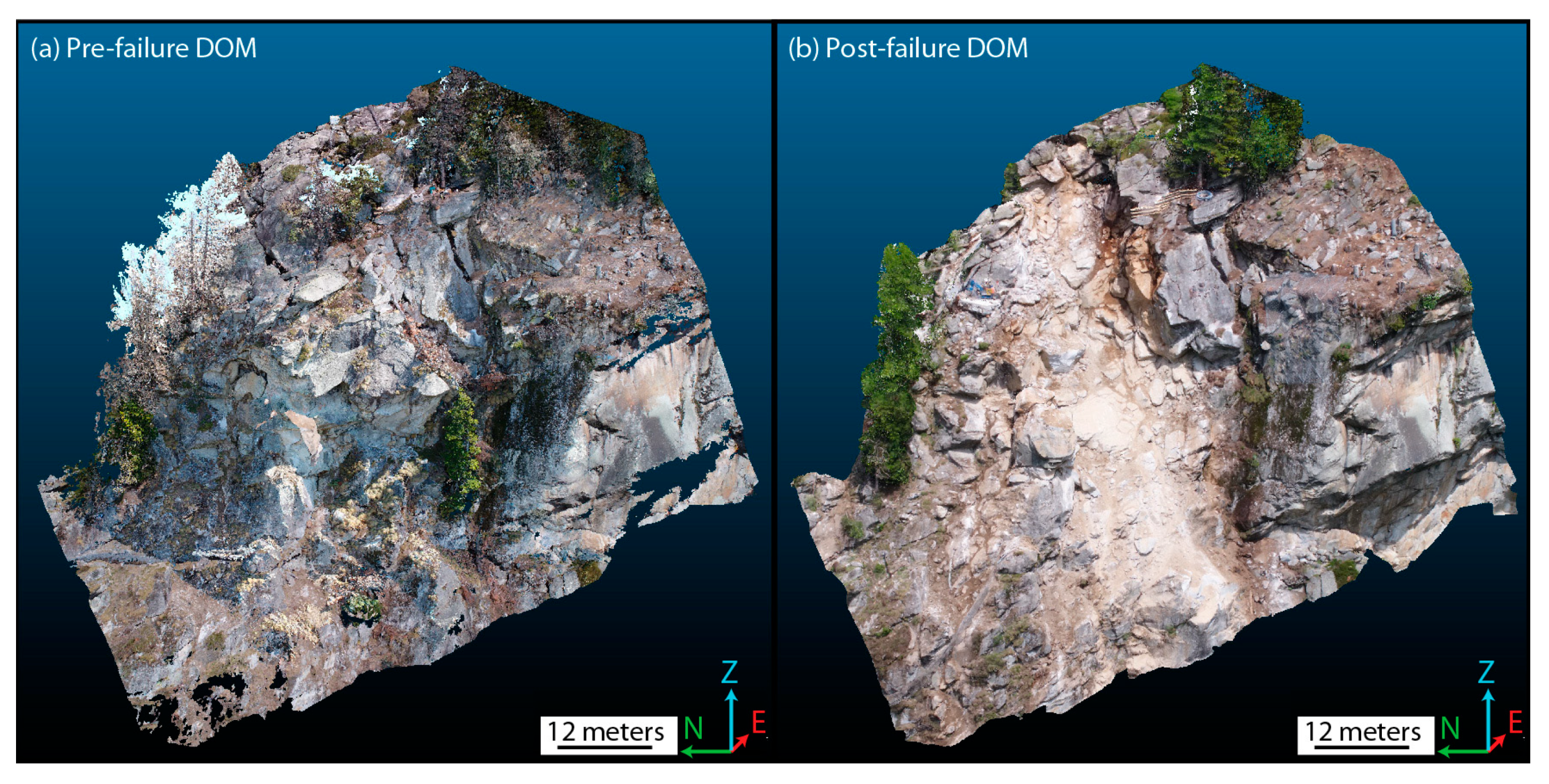
• after the landslide of May 29th, 2018 a second emergency photogrammetric survey was realized and a post-landslide Direct-Georeferenced DOM was realized with which the mode of failure and the volume of rock involved were verified;
• 30 GCPs were successively measured in the field by a laser reflector-less total station and the pre- and post-landslide photogrammetric surveys were used to realize two new GCP-georeferenced models by which the accuracy of the preceding analyses and in particular the volume estimation of the landslide was checked.

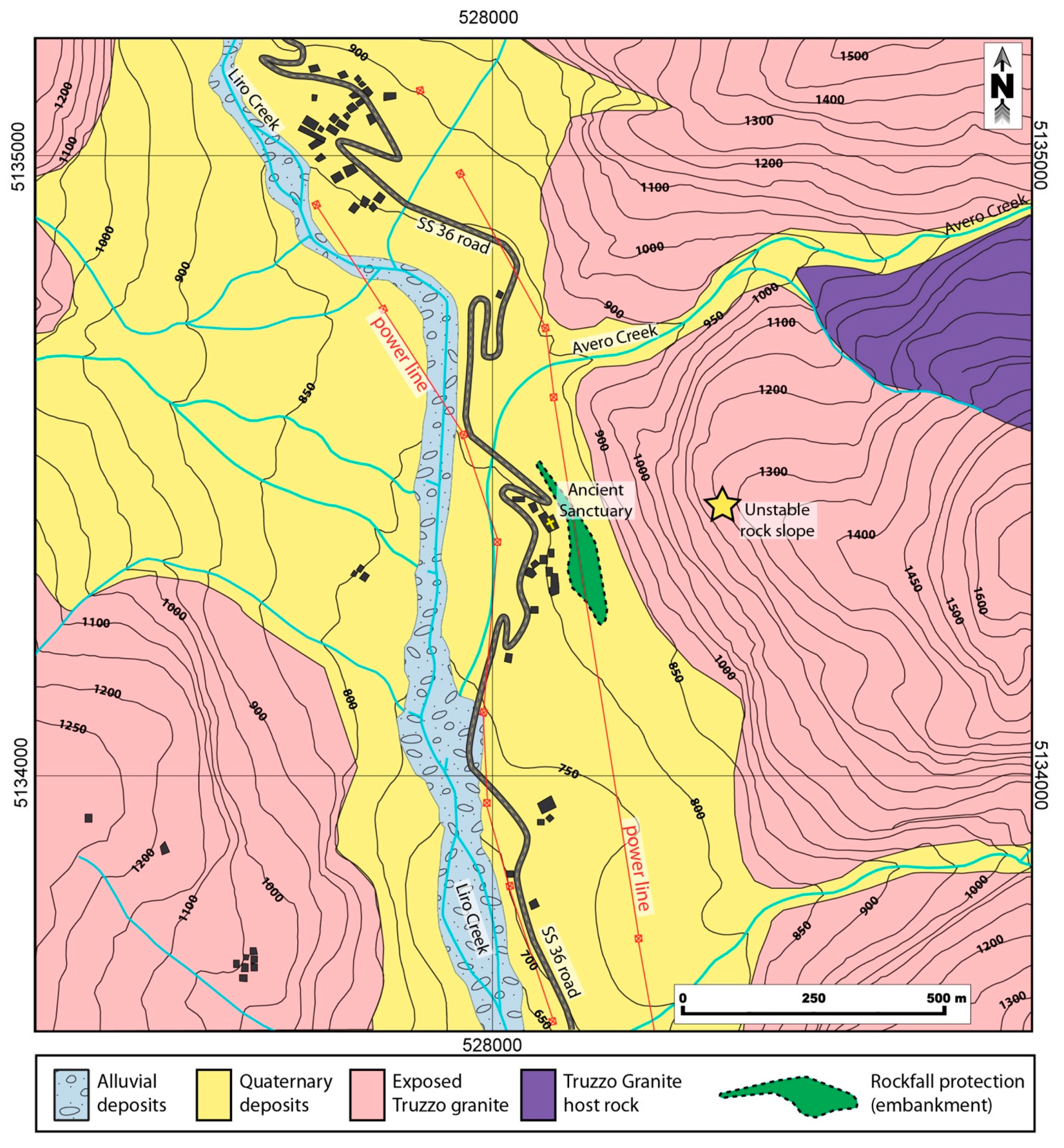
2. Site Description

The unstable rock slope studied is located along the left side of the Spluga Valley (also called San Giacomo Valley), in the San Giacomo Filippo district (the Western Alps, Sondrio Province, Italy), approximately at km 126 of the SS36 road (Figure 2).

2.1. Geological and Geomorphological Setting

The Spluga Valley, like many other Alpine valleys, was originated by the erosional phenomena connected to the Last Glacial Maximum (LGM) and it is characterized by an N-S trend, a U-shape, and steep slopes. It is included mainly in the Penninic Zone that is characterized by the presence of the Tambò and Suretta nappes and the Spluga syncline [25]. According to [26], the Spluga Valley is principally affected by the presence of two sets of lineaments related respectively to the Insubric Line, with a direction ranging from WNW-ESE to NW-SE, and to the Engadine Line, represented by a shear plane with a NE-SW direction. Moreover, N-S trending tensional fractures caused by the post-glacial rebound, and N-S shear fractures that may be related to reactivated minor pre-existed lineaments are also present.

The study slope is located onto the southern part of the Tambò nappe that is predominantly composed by polycyclic and polymetamorphic paragneiss [27]. However, the study area is totally formed by the Truzzo granite formation, a late Varisican granitic complex dated 284 ± 21 Ma (Rb-Sr whole-rock and minerals: [28]) that can be considered a monocyclic basement [25], because it is affected only by the Tertiary Alpine-deformation [29]. The study slope, as the main part of the Truzzo granite, consists of a two-micas-shaped orthogneiss with pluri-centimetric phenocrysts of potassium feldspar [25,26].

2.2. Rock Slope and Slope Toe Area

The Truzzo granite that outcrops along the rock slope is locally characterized by a metamorphic foliation that dips with a low angle toward NE (Figure 2). Different authors [26,30,31] suggested the presence of at least 3 or 4 strongly persistent discontinuity sets affecting the studied rock slope that can cause rock block instabilities. In particular, [26] identified the following sets: (i) fractures parallel to the main foliation; (ii) sub-vertical shear fractures with a WNW-ESE and NW-SE direction (as the main tectonic lineaments related to the Insubric line); (iii) N-S tension fractures, parallel to the valley (and probably related to the post-glacial rebound).

Just below the rock slope, different anthropic artefacts are endangered as the ancient Sanctuary of Gallivaggio (1598 A.D.), few houses, a restaurant, and the SS36 national road (Figure 3).

2.3. Evolution of the 29th May 2018 Failure

After the occurrence of some isolated rock block falls, the Lombardy Region Civil Protection and the Mountain Community began to build a rockfall embankment in 2008 [30]. Due to the presence of several artefacts, in particular, the SS36N national road and the Gallivaggio sanctuary, between 2011 and 2012 the Regional Agency for the Environmental Protection of Regione Lombardia (ARPA Lombardia) installed the first monitoring system. Successively, in 2016, the stability of the rock slope was also monitored by a permanent Ground-Based Interferometric Synthetic Aperture Radar (GBInSAR) system [30,31].

From the end of 2017, the GBInSAR registered an increase of the slope movements and, in particular, a dangerous acceleration from April 13th 2018 [30]. These acceleration values, together with the previous minor rockfalls, were indicating an incipient state of failure of the rock slope, where the frictional resistance of the discontinuities and rock bridges were maintained a precarious equilibrium [31]. Therefore, on April 17th an emergency RPAS survey was conducted in order to investigate the condition of the unstable rock slope, and by the obtained high-resolution DOM, quickly identify the possible failure mechanism and estimate the unstable rock volume.

On May 24th the ARPA Lombardia noticed that the acceleration trigger thresholds were exceeded and on May 29th, 35 min before the rock slope collapsed, the ARPA Lombardia sent the last warning before the landslide event [30]. As suggested by [31], the failure probably occurred by an excess of the shear stress that induced the propagation and coalescence of micro-cracks and, therefore, the breakage of the intact rock bridges along the sliding surfaces, allowing to reach failure condition of the rockfall. On May 30th, another emergency RPAS survey was conducted to verify the condition of the slope after the landslide rapidly.

3. Methodology

3.1. Digital Photogrammetric Survey

As already outlined, two different RPAS surveys were conducted before and after the landslide of the May 29th 2018 due to the difficulty and danger to investigate directly in the field the unstable portion of the rock slope (Figure 4).

The specification of the RPAS and the camera used in these surveys are described in

Table 1. RPAS and mounted-camera features.

RPAS		Camera
Type	DJI Phantom 4 Pro Quadcopter	Type	DIJ FC330X
Diagonal size [cm]	35	Sensor type	CMOS
Engines	Brushless	Sensor size [mm]	13.2 × 8.8
Rotor diameters [cm]	12	Image size [pixel]	4864 × 3648
Empty weight [kg]	1.4	Pixel size [μm]	2.61 × 2.461
		Focal length [mm]	8.8

.

The RPASDP survey on April 17th 2018 (before the event) was conducted manually, acquiring 171 images with a mean distance camera-outcrop of 35.5 m. Considering this distance and the camera features (Table 1), the mean resolution of the images is about 9 mm/pixel. The area covered by the DP survey is around 5890 m² and mainly includes the unstable portion of the rock slope.

The RPASDP survey on May 30th 2018 (the day after the primary failure) was also conducted manually, acquiring 246 images with a mean distance camera-outcrop of 191 m and a consequent mean resolution of the photos of about 39 mm/pixel. The resulting Digital Outcrop Model (DOM) covers an area of 79,957 m², showing the landslide effects on the entire slope.

3.2. Digital Outcrop Model Development

The Digital Outcrop Models (DOMs) were developed using the commercial Structure from Motion-based software, Photoscan_© (Agisoft_©, St. Petersburg, Russia). The DOMs were georeferenced with two different methods: (i) by direct-georeferentiation and (ii) by GCPs georeferentiation.

The first procedure (direct-georeferentiation) considers only the positions registered by the RPAS onboard GNSS/IMU, whereas the second build the model on the base of the locations of the GCPs recorded in the field by high-accuracy topographic instrumentation. [7,18] showed as the Direct-Georeferenced (DG) DOMs may be offset from the real coordinates with a rigid translation ranging from 10 cm to 10 m. Still, their scale and orientation are sufficiently accurate for geological purposes, with a medium homogeneous scaling of 1–5‰ and a rigid-rotation up to a maximum of 1°.

The workflow used with Photoscan© involves the following steps:

(1)

Alignment of images using their full resolution and their orientation using the GNSS/IMU-information recorded by the RPAS onboard GPS or the GCPs position measured in the field by a total station;

(2)

dense point cloud reconstruction using the high-quality setting of Photoscan (half of the image resolution);

(3)

generation of the textured mesh using the dense cloud and the high face count suggested by Photoscan© and the generic mapping and the mosaic blending modes for creating 20 texture files of 4096 × 4096 pixels.

The main feature of the developed DOMs (point clouds and meshes) are indicated in

Table 2. Statistic of the point clouds and meshes representing the slope before and after the landslide.

		Number of Points/Faces	Density of Points	Mean Face Area
Before landslide	Point cloud	28 Million	4500 pts/m2	/
	Mesh	5.6 Million	/	19 cm2
After landslide	Point cloud	21.5 Million	266 pts/m2	/
	Mesh	3.3 Million	/	493 cm2

.

The accuracy of the different DOMs is described in Section 4.2.

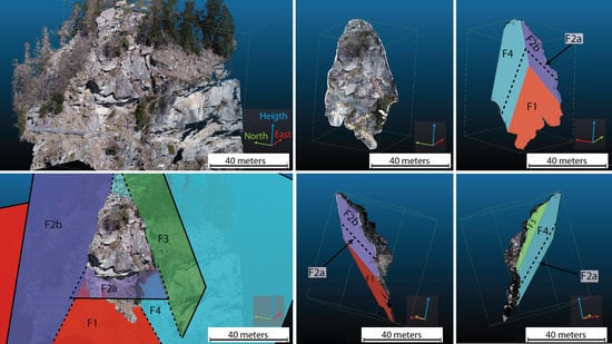
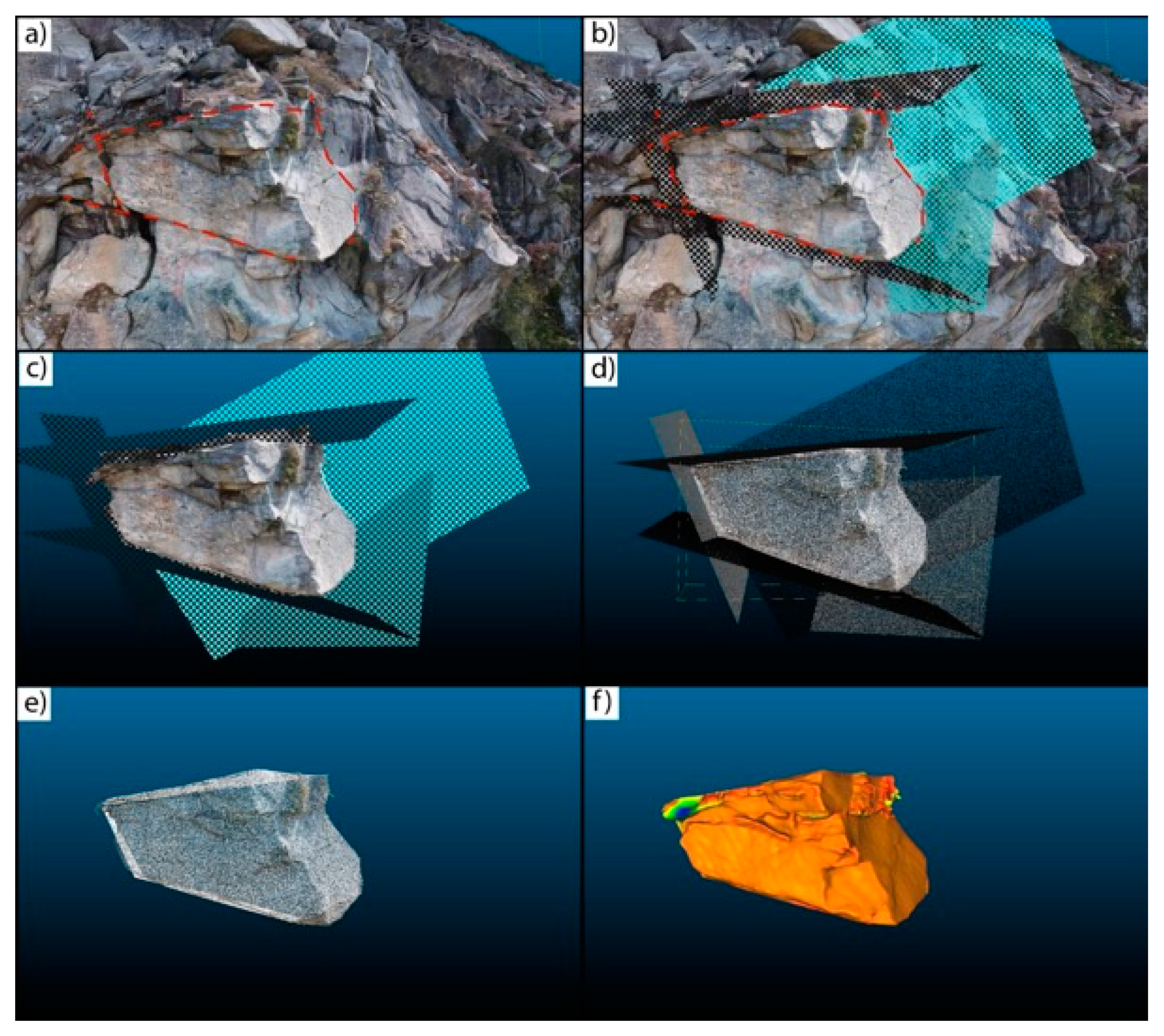
3.3. Digital Outcrop Models Analysis

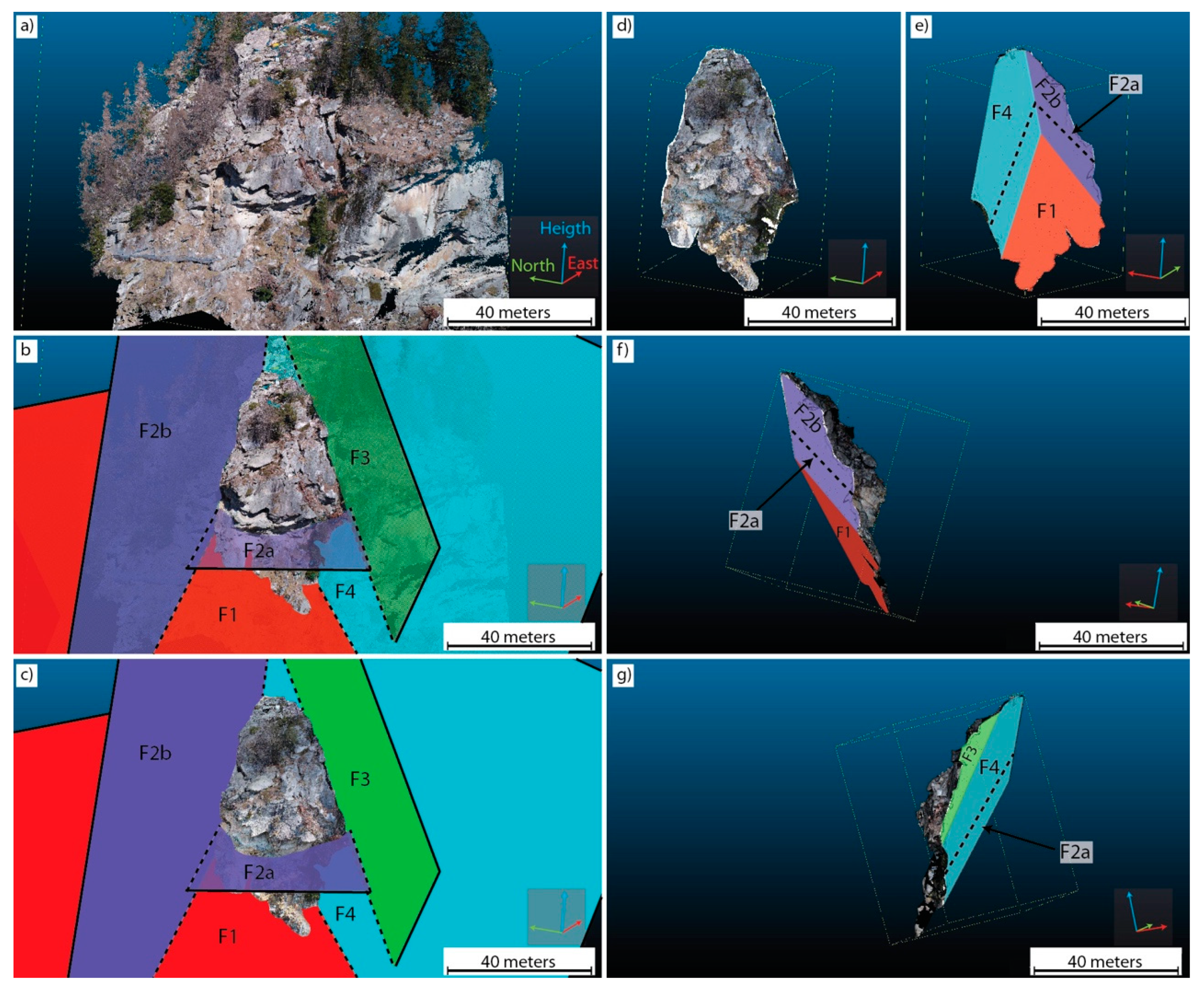
The 3D Digital Outcrop Models (DOMs) were analyzed in a 3D stereoscopic environment using the open-source software Cloud Compare v2.9 with a computer equipped with an SD2220W stereoscopic device that is composed by two separate polarized display monitors placed one above the other in a clamshell configuration, with a half-silvered glass plate bisecting the angle between the two displays.

On the pre-failure DOMs, the visible discontinuities and the traces of the potential failure surfaces affecting the rock slope were recognized and then measured directly on the point cloud by a point picking tool and the calculation of the best-fit planes. These data were projected onto a stereonet, and the principal discontinuity sets were identified.

The estimation of the possible mechanism of failure was predicted evaluating the attitude of the detected surfaces in relation to the average orientation of the slope. To estimate the volume of the potential landslide, the pre-event DOMs were analyzed through the following stages (Figure 5):

(i)

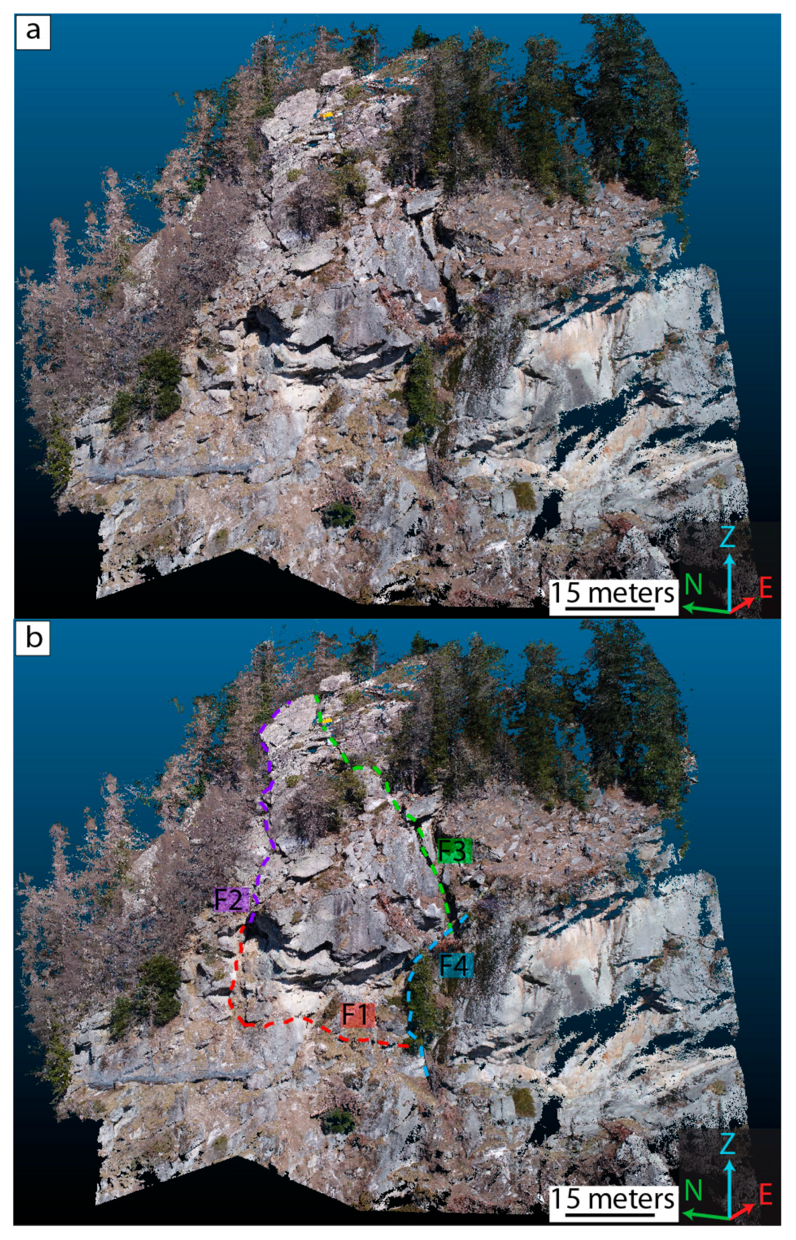
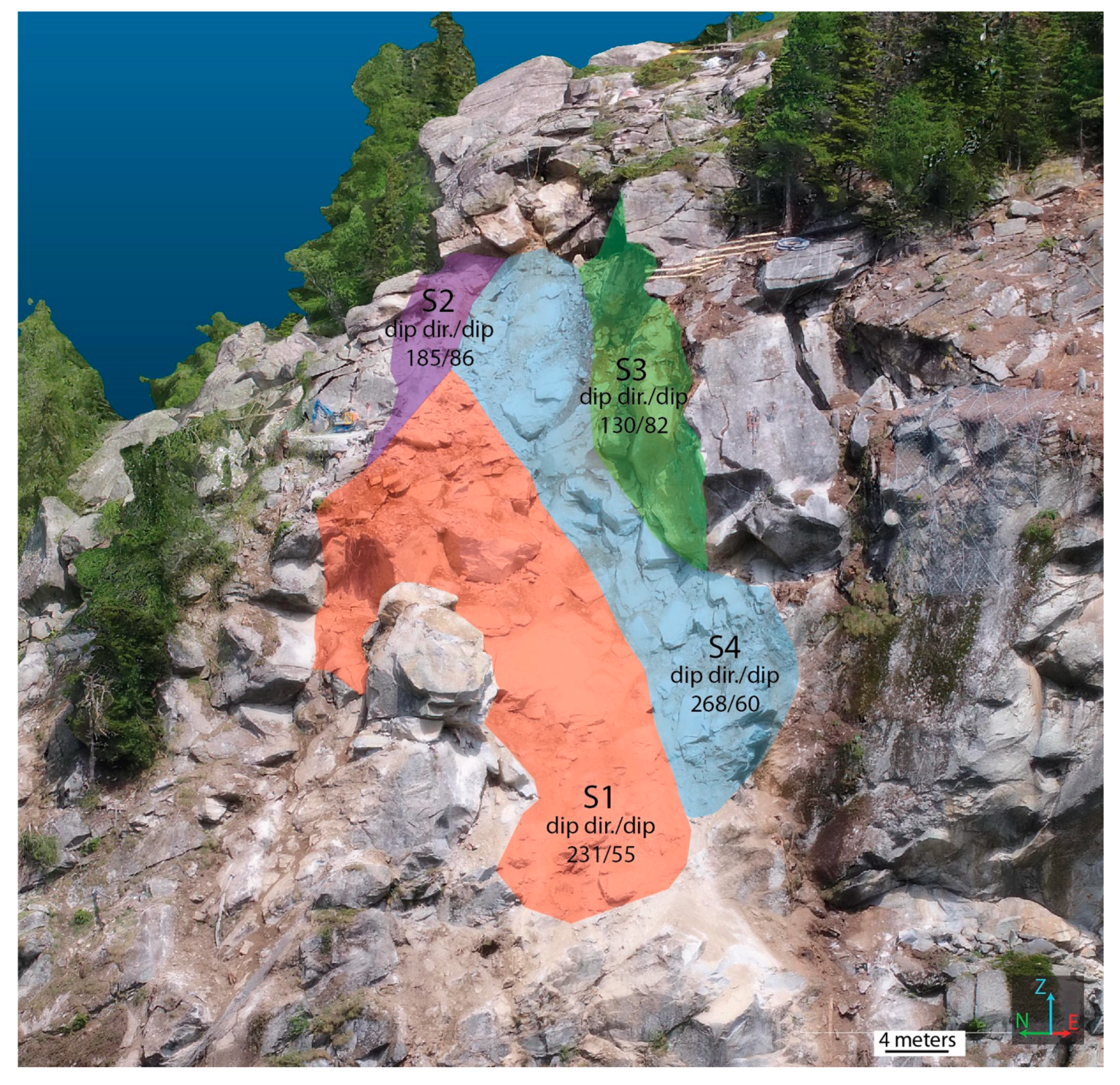
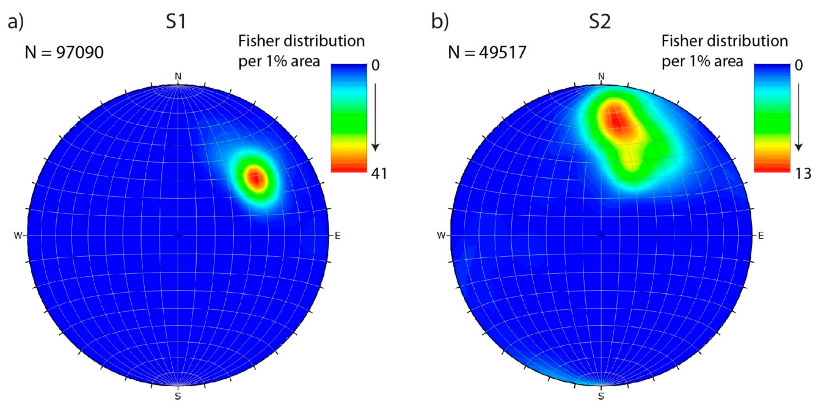
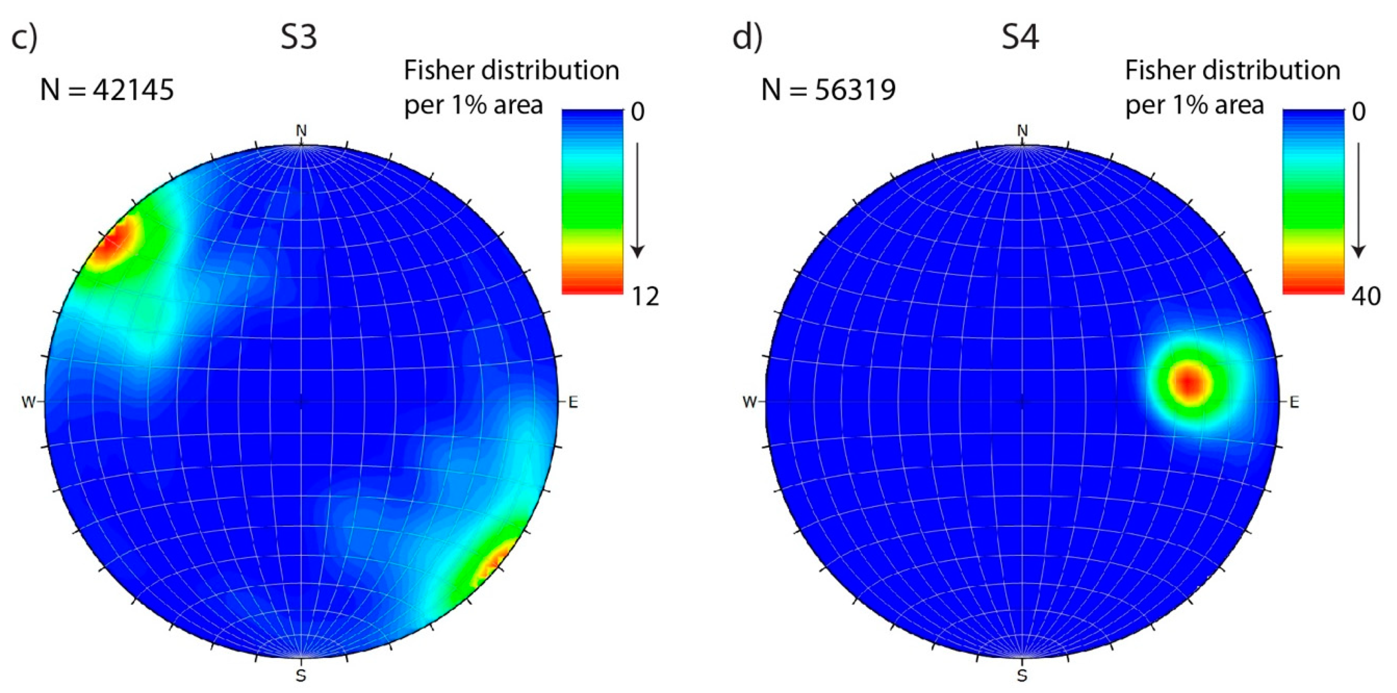
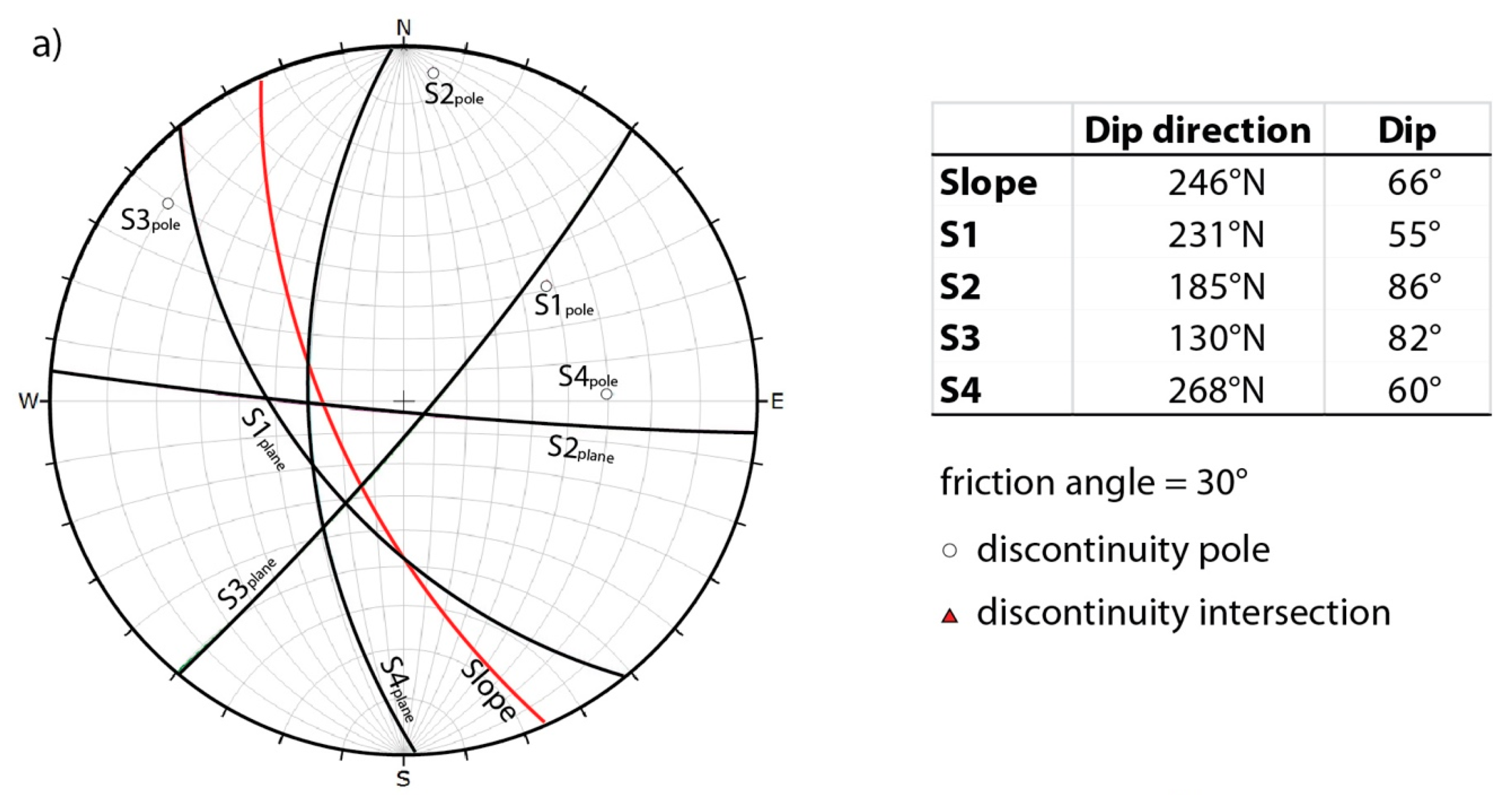
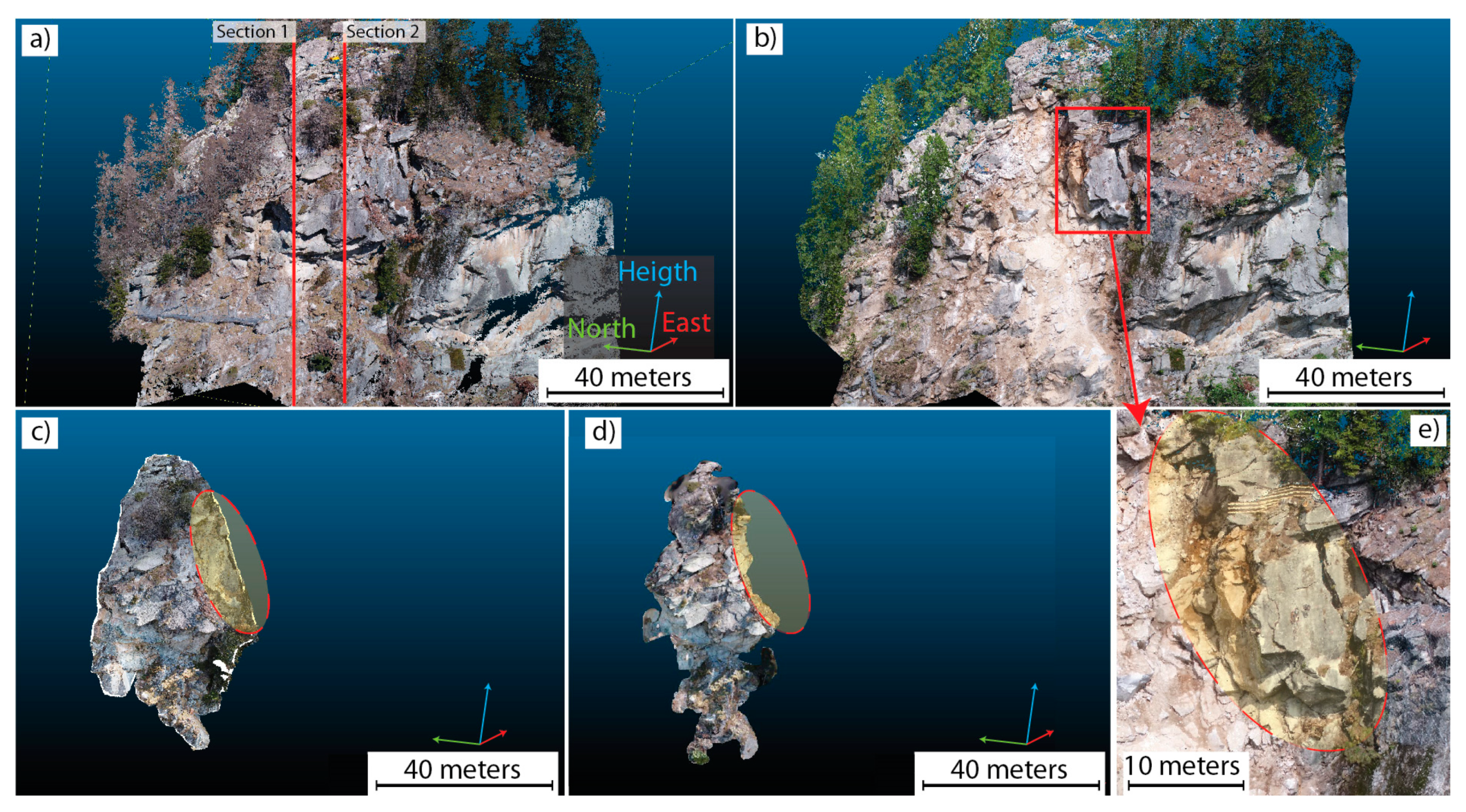
Identification and mapping of the discontinuity traces that delimit the unstable critical block and estimation of the potential sliding surfaces or intersections (Figure 5a,b);

(ii)

delimitation of the unstable portion of the slope (Figure 5c,d);

(iii)

calculation of the volume of the unstable portion of the slope (Figure 5e,f).

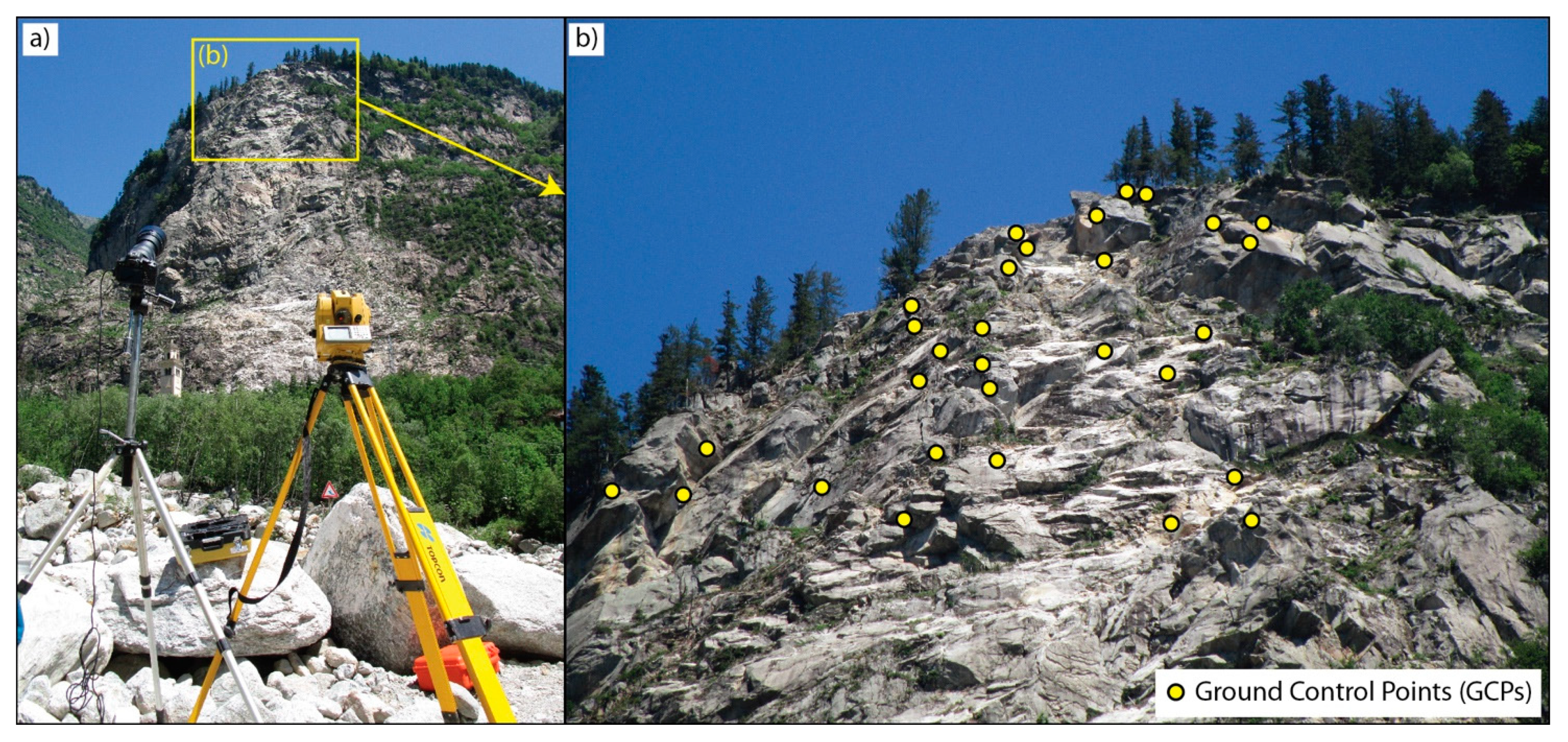
To determine the rock volume effectively involved in the landslide on May 29th 2018, the pre- and post-event DOMs were compared as described in Section 4.2.

3.4. GCP Survey

In the Gallivaggio case study, due to the emergency condition, the first evaluation of the unstable slope was done on the DOMs developed using the direct-georeferencing approach. Only some days after the collapse, the acquisition of GCPs allowed to develop DOMs with better absolute orientation and perform an uncertainty analysis (Figure 1).

The relative and absolute accuracy of the digital outcrop models were assessed using the 30 Ground Control Points (GCPs) measured in the field after the failure event of May 29th 2018 by a GPT-7001L reflector-less total station (Topcon, Tokyo, Japan) that has an accuracy of 2 + 2 × 10⁻⁶ mm (Figure 6).

We acquired 34 points, 30 on the rock wall and four benchmarks close to the total station. The position of four benchmarks has also been acquired using a 1200GPS RTK (Leica, Wetzlar, Germany). Considering the mean distance between the location of targets and the total station (900 m), and the use of reflector-less measurement mode, the accuracy can be conservatively estimated in 5 cm.

The acquired GCPs were used to develop GCP-referenced DOMs of the pre- and post-failure slopes. These DOMs were used to evaluate the accuracy of the direct-georeferenced 3D models (generated using only the positions recorded by the RPAS onboard GNSS/IMU instrumentation) and the consequent errors in estimating the volume of unstable rock.

According to [7,33], the accuracy of a DOM can be distinguished in absolute and relative accuracy. The first is represented by the error in the positioning of all 3D points of the DOM in an absolute coordinate system. In contrast, the second represents the difference in length and azimuth of the vectors that join two points on Earth, and the corresponding length and azimuth of the same vectors in the model. For example, a DOM with correct orientation and scale and an incorrect positioning in the 3D space has high relative accuracy and low absolute accuracy.

4. Results

4.1. Pre-Failure Analysis

The main goal of the pre-failure study was the identification of critical discontinuities in the most unstable sector and the estimation of the volume of the possible rockfall. From the stereoscopic inspection of the DOMs, it was possible to identify and map 134 discontinuities that can be subdivided into four different sets DS1, DS2, DS3 and DS4 (Figure 7).

However, many non-systematic fractures were observed and also the identified sets show a significant dispersion in the attitude. The mean length of the visible traces of the mapped discontinuities is 14.30 m, whereas the minimum and the maximum length are 2.40 and 60.60 m, respectively.

In addition to this fracture network, the traces of four main critical discontinuities, characterized by a high aperture (also more than 1 m) and signs of incipient instability, were identified. The combination of these fractures formed a highly unstable rock wedge (Figure 8).

The attribution of these fractures to the defined sets is problematic, especially as regards the F2 fracture, while the other three fractures can be roughly ascribed to sets DS1, DS3 and DS4. These opened fractures are rather irregular, and the measurement of their orientation is difficult (just because they are open) and show some variability. To minimize this drawback, the outcropping traces of the four fractures were sampled considering only the most reliable intersection points and four clouds of 37 (fracture F1), 66 (F2), 23 (F3), 32 (F4) points were obtained.

Then, the attitude of all the planes determined from the different possible combinations of the points of each cloud was calculated. Groups of a minimum of four points were chosen and only the planes calculated from groups with collinearity (K) < 0.8 and coplanarity (M) > 4 were considered (Figure 9), as proposed by [20].

This analysis (Figure 9) indicates that the distribution and the orientation of the fractures F1 and F4 are somewhat regular with a clear maximum of relative density with an attitude of 238°/41° and 270°/70°, respectively. On the contrary, fractures F2 and F3 show two different maxima of relative density (Figure 9b,c) suggesting that the traces of these fractures can be the envelope of two kinds of fractures with two different orientations: 227°/47° and 353°/88° for F2 and 306°/85° and 240/40° (which coincides with the orientation of F1) for F3.

According to these results, the presence of five critical discontinuities (Figure 10a) was considered (F1, F2a, F2b, F3 and F4) for the stability analysis (Figure 10c,d) and the volume calculation.

In particular, the stability analysis (Figure 10b) suggested that the discontinuity F1 and F2a could be critical for the planar sliding failure, and they can act as sliding surfaces of the rock wedge. Also, the fracture F4 has an attitude very close to being critical for planar sliding.

Moreover, four intersections between fractures could be considered critical for the wedge sliding (F1-F2a/b, F1-F3, F1-F4 and F3-F4) (Figure 10c).

Taking into account the large opening and the morphological characteristics of the potential sliding surfaces, the basic friction angle was prudently considered in the stability tests, which, in the absence of experimental data and analogy with similar lithologies [34] was deemed to be equal to 30°.

The same five fractures were used to reconstruct the geometry of the unstable rock wedge (Figure 11) except for the discontinuity F2a that plays a minor role because it does not influence the shape of the wedge, but only cuts the rock wedge in the middle.

The volume of the unstable rock wedge was estimated using the procedure described in the previous chapter, extending the potential sliding fractures visible as traces on the outcrop to delimit the internal part of the unstable block, and cutting the point cloud appropriately to delimit the external part (Figure 11).

After the selection of the points that delimit the unstable block both inside and outside the outcrop, a ‘watertight’ mesh was created using Poisson surface reconstruction plugin [32] of the CloudCompare software. The volume of the potentially unstable rock block represented by this mesh was of 8240 m³.

4.2. Post-Failure Analysis

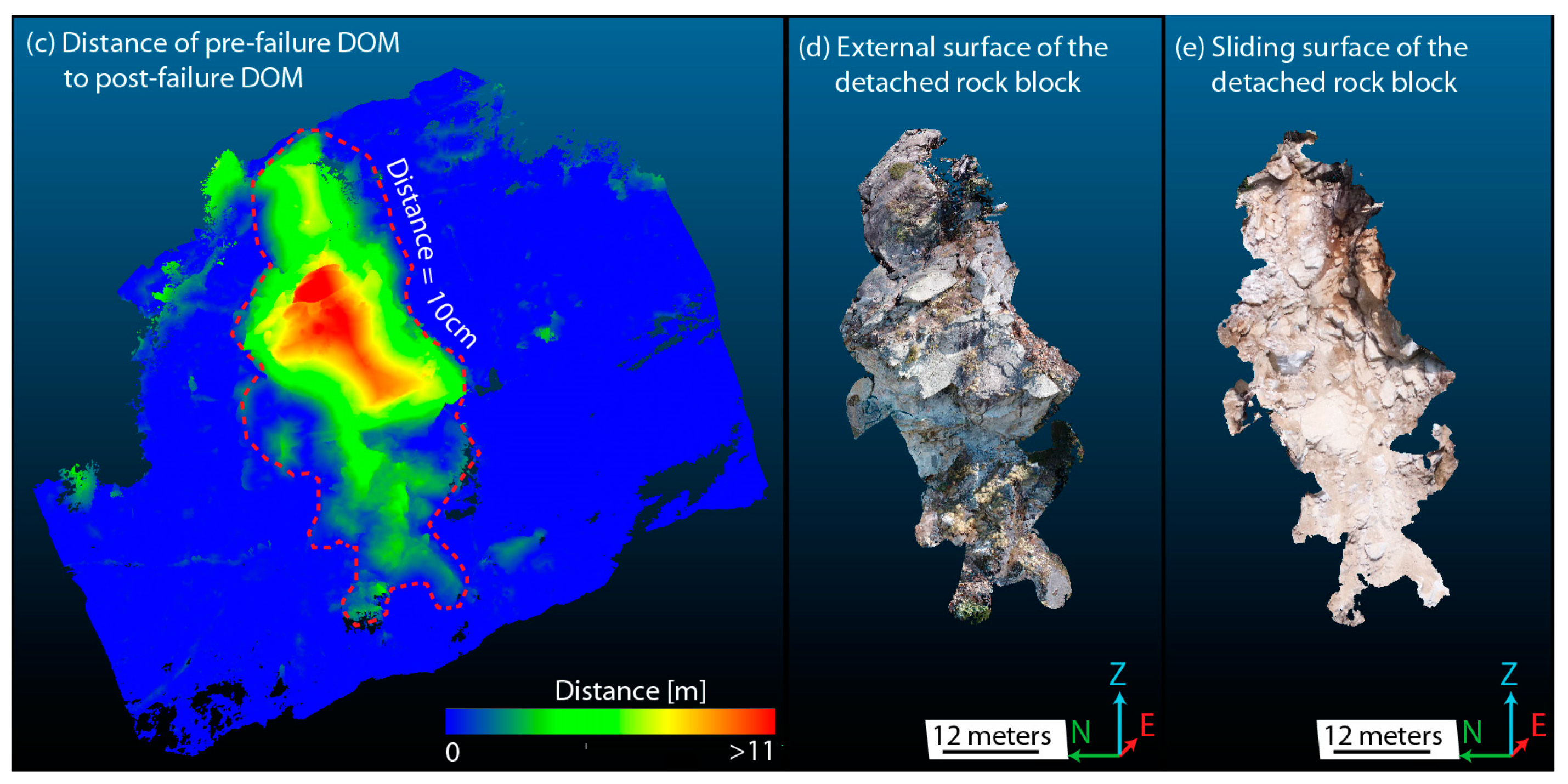
The DOMs created after the landslide of 29th May 2018 show what happened. In particular, the real mode of failure, and the rock volume effectively involved in the event and the actual failure surfaces were identified. Four principal sliding surfaces are visible (Figure 12). They are rather irregular and wavy, although with an orientation similar to that of the four fractures identified before the landslide (Figure 8 and Figure 10).

Their mean orientation was evaluated calculating the normal vectors of the points of the DOM that represent the different failure surfaces (Figure 13).

To determine the rock volume effectively involved in the landslide of May 29th 2018, it was decided to adopt a quantitative approach that minimizes the effect of the user-related bias (interpretation and manual delimitation of the sliding and the external surfaces of the rockfall), similar to those applied in [35,36,37].

The failure surfaces S2 (Figure 13b) and S3 (Figure 13c) show the higher orientation variability, and this observation confirms that they can only approximately considered as planes. Nevertheless, the comparison with the pre-event analysis confirms that the mode of failure of the landside (Figure 14) was controlled by planar sliding on S1 and S4 fractures (Figure 14b), and by wedge sliding (Figure 14c) of a complex rock wedge formed by the four discontinuity intersections (S1-S2, S1-S4, S2-S4 and S3-S4).

This approach uses the M3C2 algorithm, proposed by [38] and implemented in CloudCompare, and can be summarized in:

(a)

Selection of the portion of DOMs that represent the same rock slope area before and after the landslide (Figure 15a,b);

(b)

calculation of the distance between the pre- and post-event 3D models using the M3C2 plugin (Figure 15c), a tool that permits to calculate the distance between two DOMs and plot it onto the 3D model surfaces;

(c)

delimitation of the external and the sliding surfaces using a distance threshold of 10 cm (red lines in Figure 15d,e);

Reconstruction of a closed mesh that represents the rockfall using the Poisson surface reconstruction plugin of Cloud Compare [32] and volume calculation (Figure 16).

The distance threshold was set to 10 cm because it is the double of the uncertainty of the total station measurements. To avoid an overestimation of the rock volume, all the tall vegetation represented in the models was removed using both semi-automatic (RGB and density value of the points of the cloud) and manual procedures (point selection and elimination) proposed by [7].

At the end of this quantitative approach, the volume of the fallen rock mass thus calculated was of ca 6730 m³.

The comparison of the pre- and post-landslide 3D models shows as the estimated mode of failure (Figure 10b,c) was substantially correct, with four discontinuity intersections critical for the wedge sliding (F1-F2b, F1-F3, F1-F4, F3-F4 and S1-S2, S1-S3, S1-S4, S3-S4 onto the pre- and post-failure DOMs, respectively) (Figure 10c and Figure 14c) and two fractures (F1, F4 and S1, S4) acting as sliding surfaces (Figure 10b and Figure 14b). Nevertheless, the predicted volume of rock involved in the landslide was overestimated by around 1510 m³ (8240 vs. 6730 m³). However, accurate inspection of the post-failure 3D models shows that not all the unstable portions of the slope collapsed, as a block in precarious conditions of equilibrium is still in place (Figure 17). The volume of this block is about 809 m³. Therefore, the difference between the estimated and the real landslide volume is reduced to about 701 m³ (~10% of the real collapsed volume).

The longitudinal sections of Figure 18 indicate as the difference between the predicted and the real volume of the landslide is probably essentially influenced by the geometry of the discontinuities.

Whereas the estimated failure surfaces (D1, D2, D3 and D4) are considered planes, the real detected surfaces (S1, S2, S3 and S4) are, on the contrary, wavy and rather irregular and can be considered in many cases the envelope of discontinuities belonging to different sets.

4.3. Relative and Absolute Accuracy of the DOMs

The Direct-Georeferenced (DG) models are characterized by a low absolute accuracy with a high value of the mean errors of the coordinates (>1 m), but a low standard deviation (<0.45 m) that suggests a rigid translation (

Table 3. Statistics of the absolute accuracy of the Direct-Georeferenced DOMs. The X, Y and Z components are represented by the real value, whereas the planimetric component (XY) is represented by its absolute value.

	Easting (X)	Northing (Y)	Planar (XY)	Elevation (Z)
Mean error (m)	−2.510	−1.327	2.867	5.646
St. Deviation (m)	0.120	0.446	0.216	0.309

). On the other hand, GCP-georeferenced DOMs show a high level of absolute accuracy (

Table 4. Ground Control Points (GCPs) and ChecK Points (CKPs) errors of the GCP-georeferenced DOM. The values are expressed in centimetres.

		Easting (X)	Northing (Y)	Planar (XY)	Elevation (Z)
GCPs	Mean error (cm)	3.4	4.8	5.9	3.5
	St. Deviation (cm)	2.5	3.6	4.4	2.7
CKPs	Mean error (cm)	4.4	8.7	9.7	4.8
	St. Deviation (cm)	4.1	6.5	7.7	3.5

).

To analyze the relative accuracy of the DG DOMs, the length and the orientation (azimuth and plunge) of the 435 vectors that join all the possible couples of GCPs measured by the total station have been compared with those calculated from the DG models. The results are reported in

Table 5. Statistics of the differences between the 435 GCP-couples vector length and orientation (azimuth and plunge) measured by the total station and estimated from the direct georeferenced model.

	Length (m)	Length (‰)	Azimuth (°)	Plunge (°)
Mean	0.285	4.5‰	0.6	0.1
St. Deviation	0.358	5‰	0.6	0.6
Median	0.283	4.5‰	0.6	0.1

.

The maximum angular difference in attitude (Table 5) of the vectors is <1°, while their mean difference in length is about 4.5‰ (Figure 19).

It is essential to highlight that a 2D error of 5‰ on each axis corresponds to a 3D volumetric error of 1.5% that was confirmed by the difference of the volume of the landslide calculated in the direct-referenced and GCP-referenced models (6730 m³ vs. 6864 m³; ca. 1.7%).

These results confirm that the Direct-Georeferenced models are generally correctly oriented and usable for most geological and geoengineering purposes [7].

5. Discussion

The slope of Gallivaggio that is located along the left side of the Spluga Valley (Sondrio Province, Western Alps, Italy) was investigated by Remote Piloted Aerial System (RPAS) Digital Photogrammetric (DP) surveys before and after the 29th May 2018 rock landslide. Two pairs of 3D Digital Outcrop Models (DOMs) were realized. The Direct-Georeferenced models were developed during the emergency, before and after the event, in a relatively short time, without measuring Ground Control Points (GCPs), but using only the positions of the photographs registered by the RPAS onboard GPS. On the contrary, the GCP-georeferenced models were developed using the locations of 30 GCPs measured in the field by a total station.

The analysis of the pre-landslide models was aimed to define the fracture network affecting the slope, the potential sliding surfaces, the possible failure mechanism and the volume of rock possibly involved in the landslide. The analysis was particularly complex due to the irregular fracture network of the slope and the presence of potential sliding surfaces open, poorly exposed and challenging to measure.

5.1. Case Specific Evaluations

Four main discontinuity sets were recognized (see also [26]). Set DS1 is attributable to NW-SE and WNW-ESE sub- vertical shear fractures (as the main tectonic lineaments related to the Insubric line), set DS2 represents the fractures that dip ENE and are sub- parallel to the main foliation, set DS3 is NE-SW trending as the sub-vertical shear fractures related to the Engandine Line and set DS4 coincides with N-S tension fractures parallel to the principal valley. It is probably related to the post-glacial rebound of the area. Moreover, by the analysis of the pre-failure DOMs, four potential failure surfaces were identified (F1, F2, F3 and F4 – Figure 10), whose attitudes and intersections can induce both planar and wedge sliding. The measurement of these open and partially loose fractures was verified by sampling all the most reliable points of their traces on the outcrop. Finally, the volume of the unstable rock mass delimited by the intersection of these fractures was calculated in 8240 m³.

The comparison between these results with what happened after the landslide, and that was quantified analyzing the post-failure models allows to make the following considerations:

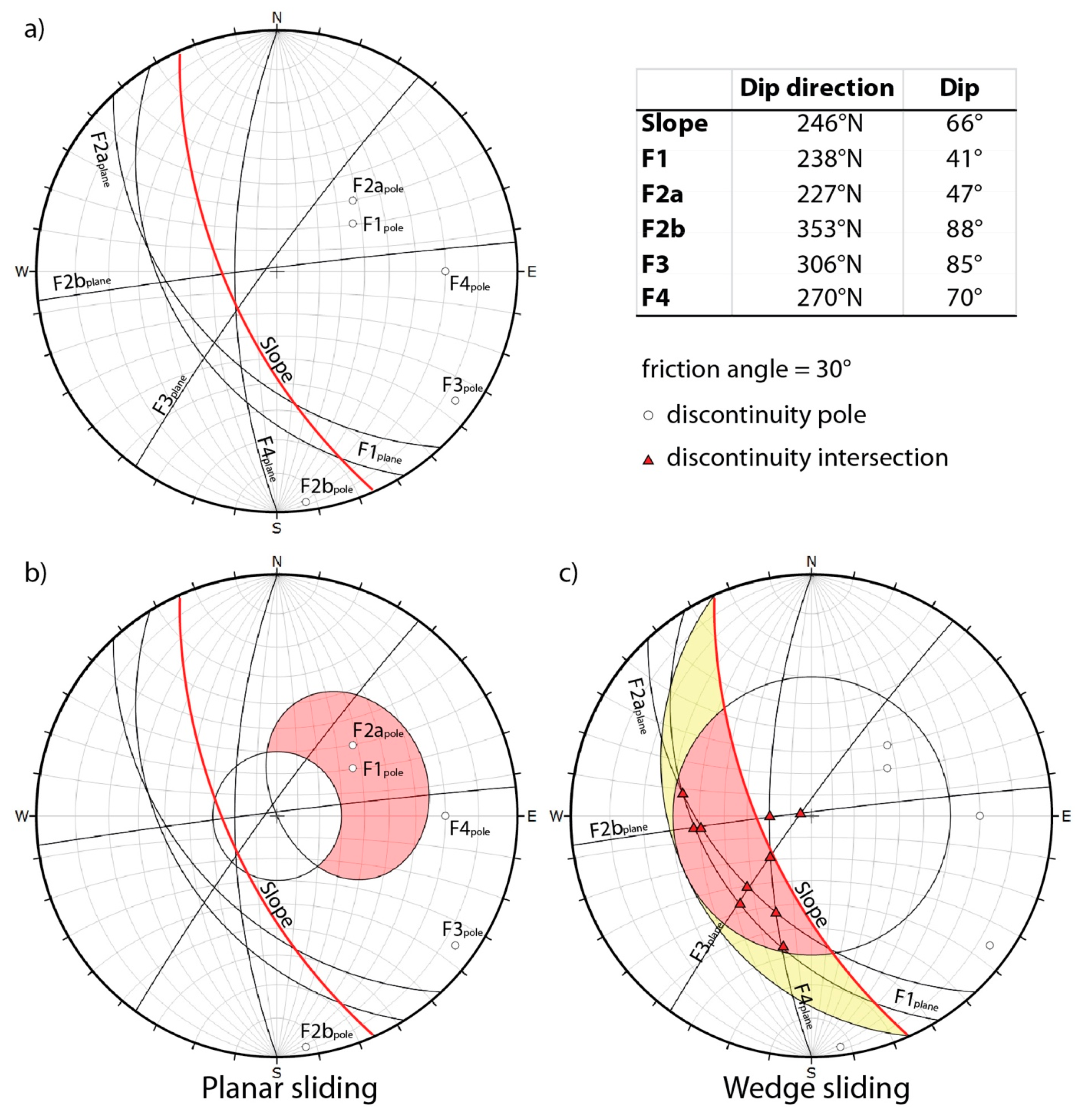
• The discontinuities really involved in the landside (S1, S2, S3 and S4 - Figure 12 and Figure 13) and detected in the post-failure DOMs have similar orientations, and the mechanism of failure of the landslide was correctly determined, with two fractures (F1, F4 and S1, S4 onto the pre- and post-failure DOMs, respectively) acting as sliding surfaces (Figure 10b and Figure 14b) and 4 discontinuity intersections critical for the wedge sliding (F1-F2b, F1-F3, F1-F4, F3-F4 and S1-S2, S1-S3, S1-S4, S3-S4) (Figure 10c and Figure 14c);
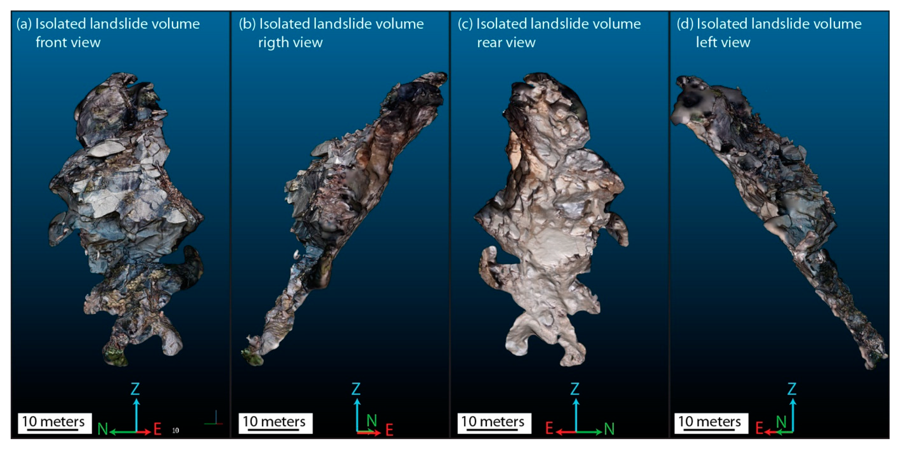
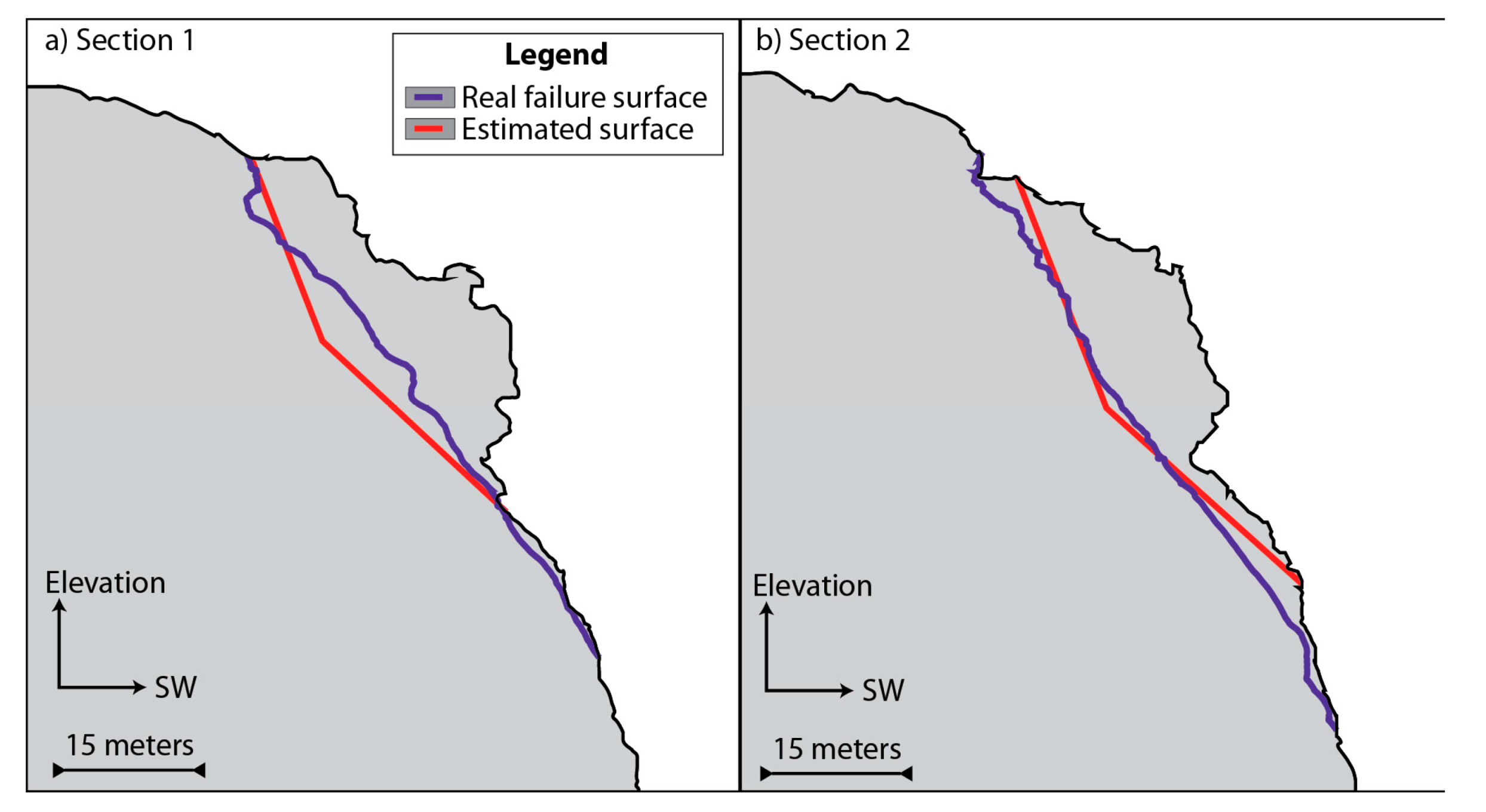
• the predicted volume of the landslide was overestimated by about 10% (~700 m³), considering that a rock block of about 809 m³ is in precarious conditions of equilibrium, but still in place (Figure 17). This difference seems due to the geometry of the effective failure surfaces that are wavy and rather irregular because probably they are the envelope of differently oriented fractures, while the sliding surfaces considered in the calculation were assumed to be planar;
• the differences in fracture measurements and the calculation of the volume of unstable rock performed on the Direct-Georeferenced (DG) and on the GCPs-georeferenced models are negligible from a geological point of view. This confirms the satisfying relative accuracy of the DG DOMs that shows an error in orientation <1°, and in the length of 4.5‰. Even the difference in the volume calculation was only 1.7% (134 m³). However, it must be considered that the absolute accuracy of these models is limited as they are affected by displacement errors of even a few meters (in this case around 2 m and 5 m of planar and vertical displacement, respectively), while the GCP-georeferenced models showed high absolute accuracy, with errors on the axes X, Y and Z always around 5 cm (similar to the total station accuracy).

5.2. Uncertainty Evaluation and Analysis

The main steps of the uncertainty analysis performed in this work, from the pre-failure estimation to the post-failure and GCP-based analysis, are shown in Figure 1.

In general, the RPAS photogrammetric survey gives the best results when coupled with GCP measurements by high-accuracy topographic instrumentation, allowing to obtain 3D models with a centimetric accuracy (Table 4) and, therefore, to map discontinuities, and to estimate and calculate the rockfall mechanisms and volume with high precision.

Notwithstanding, if the risk of a collapse of the monitored area is high, it is often difficult/impossible and extremely dangerous to perform a GCP-survey. Therefore, the 3D models must be directly-georeferenced using the RPAS position registered by the onboard instrumentation. In our research we demonstrate as the effects of the direct-georeferencing onto the absolute and relative accuracies of DOMs and therefore onto the reliability of the orientation and length measurements are in good agreement with the results obtained in other studies ([7,18]). We showed as whereas the absolute accuracy of these 3D models is low, the relative one is generally high: the length and orientation errors are equal or smaller than 5‰ and 1°, respectively, while the calculation of the rockfall volume can produce an error of 1.7%. This error can be considered as the instrumental error of direct-georeferencing RPAS photogrammetry approach and depends on the accuracy of the RPAS onboard instrumentation.

During the evaluation of the possible rockfall volume performed before the failure event onto a direct-georeferenced DOM, the instrumental error can be neglected in comparison to other kinds of uncertainties that are related to the procedures used to analyze and measure the features of the rock slope on the DOMs (methodological errors). In the literature, these errors are indicated as intrinsically connected to the discontinuity trace mapping [19], discontinuity attitude estimation ([20,21,22,23]) and interpolation of the mesh representing the unstable rock block whose volume is to be calculated [24].

Reference [19] claims that the discontinuity trace mapping based on DOMs can produce errors that are at least the double of the resolution of the digital models because of the ambiguity of the colours of the adjacent pixels. In our research, we tried to overcome this drawback realizing a high-resolution DOM (9 mm/pixel) and selecting only the most reliable outcrop-discontinuity intersection points, avoiding any type of automatic tracing of discontinuities.

Other possible sources of error lie in the orientation estimates produced by plane fitting that can be highly uncertain, especially when observed data are approximately collinear [21]. Some authors [20,21,22,23] have proposed different methods based on geometrical parameters and statistical analysis of the sampled points to minimize these possible errors and to evaluate the accuracy of the results. Our approach involved the accurate detection of the best points visible along the traces of the sliding surfaces and the calculation of all possible planes considering only groups of a minimum of four points characterized by collinearity (K) < 0,8 and coplanarity (M) > 4 (Figure 9), as proposed by [20]. This procedure proved to be effectively adequated because the predicted variability in the orientation of the discontinuities (Figure 9) was similar to the real variability detected onto the post-failure DOMs (Figure 13).

The reconstruction of the mesh that must represent the unstable or the fallen rock block is commonly realized by the conversion of a point cloud to a triangulated mesh. For accurate volume calculations, the triangulated mesh needs to be watertight (without missing triangles or surface holes), free of intersecting triangles and have consistent normal vectors, with correct topology. [24] claim that the accuracy of the mesh interpolation can be influenced by the density of points cloud representing the rock block and the algorithm chosen of reconstruction. Some reconstruction algorithms were implemented using a synthetic rockfall object and three natural rockfall events. The comparison shows that the calculated volume can also vary by 10%, even considering only meshes with a similar high density of points [24]. In our research to minimize this effect, we used very dense point clouds (10,000 pts/m²) representing the rock blocks, the Poisson surface reconstruction method that, as reported by [39,40], gives the best results for dense point cloud and closed geometry, as a rock block.

Nevertheless, the volume estimation of the unstable portion of the rock slope of Gallivaggio that is characterized by an irregular fracture network was affected by an error of 10%. This error is mainly influenced by the assumption that the potential sliding surfaces are planar. In contrast, the real ones are wavy and irregular because of the presence of rock bridge and minor discontinuities that can make the failure surface complex [41].

Therefore, it is essential to emphasize that, during the emergency condition, the GCP-survey can become superfluous because the major influence on the uncertainty of the rockfall volume is not due to the instrumental error (1.7%) but to the methodological one (10%). In particular, due to the consideration of the critical failure surfaces as planar (Figure 18).

Notwithstanding, it is important to consider that using the proposed methodology it is possible to correctly estimate the orientation variability of the critical fracture (Figure 9 and Figure 13) and, therefore, to accurately estimate the failure mechanisms (Figure 10 and Figure 14).

6. Conclusions

Digital Outcrop Models developed by photogrammetric surveys of RPAS equipped with onboard GNSS/IMU can be considered powerful tools to analyze the fracture network and the stability conditions of rock slopes, especially when slopes are inaccessible, highly unstable and dangerous. This methodology permits to acquire information from inaccessible areas in a short time, with a dramatic increase of the data principally due to the possibility to examine large portions of the slope using a safe methodology, and with substantial time-saving respect to the classic geomechanical field-based analyses. RPAS photogrammetric surveys, compared to Terrestrial Laser Scanner investigations also have the great advantage to avoid holes in the reconstruction of the point cloud and mesh of a DOM because the occlusion effect that can characterize slope with complex geometry and without optimal terrestrial viewpoints, like the case of Gallivaggio. Hole-filling procedures are one of the major problems for a correct mesh reconstruction and can produce errors in the volume estimations [24].

The DOMs developed by a direct-georeferencing procedure (i.e., without measuring ground control points, but using only the positions of the photographs registered by the RPAS onboard GPS) are generally correctly oriented and usable for most geological purposes [7]. In particular, it is possible to obtain information on unstable slopes and perform reliable stability analyses and volume estimations, especially during the emergency in a short time, also without programming a survey of acquisition of ground control points.

The procedure used in the study of Gallivaggio rockfall is aimed to estimate the volume of rock potentially involved in a landslide proved correct and substantially reliable also if applied to a slope affected by irregular and rather dispersed sets of fractures. It consists of five steps: (1) identification and mapping of the critical discontinuities; (2) fitting of 3D mean discontinuity planes after an evaluation of the uncertainties of their measurements; (3) delimitation of the surface of the unstable wedge; (4) creation and correction of the point cloud representing the unstable wedge; (5) creation and calculation of a closed 3D volume.

In this case study, the errors in the estimation of the volume are: 1.7% related to the use of direct approach and 10% linked to the uncertainty in the definition of the sliding surface due to the presence of irregularities. The uncertainty due to the direct approach can be avoided by the use of GCPs. The geological uncertainty is not entirely preventable. To evaluate the variability of the measurements of the discontinuities taken on the pre-failure DOMs, their outcropping traces were sampled and transformed into point clouds, and the attitude of all the planes determined from the different possible combinations of four points (characterized by a reduced coplanarity and collinearity) of each cloud was calculated. The analysis of the results allows determining the best-fit plane of every discontinuity and its representativeness and reliability. This procedure appears particularly necessary to establish the orientation of a single plane and characterized by a non-regular geometry or in the presence of a rock mass non-regularly fractured. However, the hardly predictable orientation and geometry of the not visible parts of the sliding surfaces, at least, in this case, prevent a more precise prediction of the volume of rock subject to failure.

References

1. Powers, P.S.; Chiarle, M.; Savage, W.Z. A digital photogrammetric method for measuring horizontal surficial movements on the Slumgullion earthflow, Hinsdale County, Colorado. Comput. Geosci. 1996, 22, 651–663. [Google Scholar] [CrossRef]
2. Jaboyedoff, M.; Oppikofer, T.; Abellán, A.; Derron, M.H.; Loye, A.; Metzger, R.; Pedrazzini, A. Use of LIDAR in landslide investigations: A review. Nat. Hazards 2012, 61, 5–28. [Google Scholar] [CrossRef] [Green Version]
3. Westoby, M.J.; Brasington, J.; Glasser, N.F.; Hambrey, M.J.; Reynolds, J.M. ‘Structure-from-Motion’ photogrammetry: A low-cost, effective tool for geoscience applications. Geomorphology 2012, 179, 300–314. [Google Scholar] [CrossRef] [Green Version]
4. Humair, F.; Pedrazzini, A.; Epard, J.L.; Froese, C.R.; Jaboyedoff, M. Structural characterization of Turtle mountain anticline (Alberta, Canada) and impact on rock slope failure. Tectonophysics 2013, 605, 133–148. [Google Scholar] [CrossRef]
5. Spreafico, M.C.; Francioni, M.; Cervi, F.; Stead, D.; Bitelli, G.; Ghirotti, M.; Girelli, V.A.; Lucente, C.C.; Tini, M.A.; Borgatti, L. Back Analysis of the 2014 San Leo landslide using combined terrestrial laser scanning and 3D distinct element modelling. Rock Mech. Rock Eng. 2016, 49, 2235–2251. [Google Scholar] [CrossRef] [Green Version]
6. Menegoni, N.; Meisina, C.; Perotti, C.; Crozi, M. Analysis by UAV Digital Photogrammetry of Folds and Related Fractures in the Monte Antola Flysch Formation (Ponte Organasco, Italy). Geosciences 2018, 8, 299. [Google Scholar] [CrossRef] [Green Version]
7. Menegoni, N.; Giordan, D.; Perotti, C.; Tannant, D.D. Detection and geometric characterization of rock mass discontinuities using a 3D high-resolution digital outcrop model generated from RPAS imagery–Ormea rock slope, Italy. Eng. Geol. 2019, 252, 145–163. [Google Scholar] [CrossRef]
8. Sturzenegger, M.; Stead, D. Close-range terrestrial digital photogrammetry and terrestrial laser scanning for discontinuity characterization on rock cuts. Eng. Geol. 2009, 106, 163–182. [Google Scholar] [CrossRef]
9. Colomina, I.; Molina, P. Unmanned aerial systems for photogrammetry and remote sensing: A review. ISPRS J. Photogramm. Remote Sens. 2014, 92, 79–97. [Google Scholar] [CrossRef] [Green Version]
10. Francioni, M.; Salvini, R.; Stead, D.; Coggan, J. Improvements in the integration of remote sensing and rock slope modelling. Nat. Hazards 2018, 90, 975–1004. [Google Scholar] [CrossRef] [Green Version]
11. Bemis, S.P.; Micklethwaite, S.; Turner, D.; James, M.R.; Akciz, S.; Thiele, S.T.; Bangash, H.A. Ground-based and UAV-based photogrammetry: A multi-scale, high-resolution mapping tool for structural geology and paleoseismology. J. Struct. Geol. 2014, 69, 163–178. [Google Scholar] [CrossRef]
12. Giordan, D.; Adams, M.; Aicardi, I.; Alicandro, M.; Allasia, P.; Baldo, M.; De Berardinis, P.; Dominici, D.; Godone, D.; Hobbs, P.; et al. The use of unmanned aerial vehicles (UAVs) for engineering geology applications. Bull. Eng. Geol. Environ. 2020, 1–45. [Google Scholar] [CrossRef] [Green Version]
13. Turner, D.; Lucieer, A.; Wallace, L. Direct georeferencing of ultrahigh-resolution UAV imagery. IEEE Trans. Geosci. Remote Sens. 2013, 52, 2738–2745. [Google Scholar] [CrossRef]
14. Nikolakopoulos, K.G.; Koukouvelas, I.; Argyropoulos, N.; Megalooikonomou, V. Quarry monitoring using GPS measurements and UAV photogrammetry. In Earth Resources and Environmental Remote Sensing/GIS Applications VI; International Society for Optics and Photonics: Toulouse, France, 2015; p. 96440J. [Google Scholar] [CrossRef]
15. James, M.R.; Robson, S.; Smith, M.W. 3-D uncertainty-based topographic change detection with structure-from-motion photogrammetry: Precision maps for ground control and directly georeferenced surveys. Earth Surf. Process. Landf. 2017, 42, 1769–1788. [Google Scholar] [CrossRef]
16. Forlani, G.; Dall’Asta, E.; Diotri, F.; Cella, U.M.D.; Roncella, R.; Santise, M. Quality assessment of DSMs produced from UAV flights georeferenced with onboard RTK positioning. Remote Sens. 2018, 10, 311. [Google Scholar] [CrossRef] [Green Version]
17. Carbonneau, P.E.; Dietrich, J.T. Cost-effective non-metric photogrammetry from consumer-grade sUAS: Implications for direct georeferencing of structure from motion photogrammetry. Earth Surf. Process. Landf. 2017, 42, 473–486. [Google Scholar] [CrossRef] [Green Version]
18. Cawood, A.J.; Bond, C.E.; Howell, J.A.; Butler, R.W.; Totake, Y. LiDAR, UAV or compass-clinometer? Accuracy, coverage and the effects on structural models. J. Struct. Geol. 2017, 98, 67–82. [Google Scholar] [CrossRef]
19. Tziavou, O.; Pytharouli, S.; Souter, J. Unmanned Aerial Vehicle (UAV) based mapping in engineering geological surveys: Considerations for optimum results. Eng. Geol. 2018, 232, 12–21. [Google Scholar] [CrossRef] [Green Version]
20. Fernández, O. Obtaining a best fitting plane through 3D georeferenced data. J. Struct. Geol. 2005, 27, 855–858. [Google Scholar] [CrossRef]
21. Seers, T.D.; Hodgetts, D. Probabilistic constraints on structural lineament best fit plane precision obtained through numerical analysis. J. Struct. Geol. 2016, 82, 37–47. [Google Scholar] [CrossRef]
22. Thiele, S.T.; Grose, L.; Cui, T.; Cruden, A.R.; Micklethwaite, S. Extraction of high-resolution structural orientations from digital data: A Bayesian approach. J. Struct. Geol. 2019, 122, 106–115. [Google Scholar] [CrossRef]
23. Quinn, D.P.; Ehlmann, B.L. A PCA-based framework for determining remotely sensed geological surface orientations and their statistical quality. Earth Space Sci. 2019, 6, 1378–1408. [Google Scholar] [CrossRef] [PubMed]
24. Bonneau, D.; DiFrancesco, P.M.; Hutchinson, D.J. Surface Reconstruction for Three-Dimensional Rockfall Volumetric Analysis. ISPRS Int. J. Geo-Inf. 2019, 8, 548. [Google Scholar] [CrossRef] [Green Version]
25. Marquer, D. Structures et cinématique des déformations alpines dans le granite de Truzzo (Nappe de Tambo: Alpes centrales suisses). Eclogae Geol. Helv. 1991, 84, 107. [Google Scholar]
26. Ferrari, F.; Apuani, T.; Giani, G.P. Applicazione di modelli cinematici per lo studio di frane di crollo in media Val San Giacomo (SO). Geoing. Ambient. Min. 2011, XLVIII, 55–64. [Google Scholar]
27. Ferrari, F.; Apuani, T.; Giani, G.P. Rock Mass Rating spatial estimation by geostatistical analysis. Int. J. Rock Mech. Min. Sci. 2014, 70, 162–176. [Google Scholar] [CrossRef] [Green Version]
28. Marquer, D.; Baudin, T.; Peucat, J.J.; Persoz, F. Rb-Sr mica ages in the Alpine shear zones of the Truzzo granite: Timing of the Tertiary alpine PT-deformations in the Tambo nappe (Central Alps, Switzerland). Eclogae Geol. Helv. 1994, 87, 225–229. [Google Scholar]
29. Baudin, T.; Marquer, D.; Persoz, F. Basement-cover relationships in the Tambo nappe (Central Alps, Switzerland): Geometry, structure and kinematics. J. Struct. Geol. 1993, 15, 543–553. [Google Scholar] [CrossRef]
30. Dei Cas, L.; Pastore, M.L.; Rivolta, C. Gallivaggio landslide: The geological monitoring, of a rock cliff, for early warning system. Ital. J. Eng. Geol. Environ. 2018, 18, 41–55. [Google Scholar] [CrossRef]
31. Carlà, T.; Nolesini, T.; Solari, L.; Rivolta, C.; Dei Cas, L.; Casagli, N. Rockfall forecasting and risk management along a major transportation corridor in the Alps through ground-based radar interferometry. Landslides 2019, 16, 1425–1435. [Google Scholar] [CrossRef] [Green Version]
32. Kazhdan, M.; Hoppe, H. Screened poisson surface reconstruction. ACM Trans. Graph. 2013, 32, 29. [Google Scholar] [CrossRef] [Green Version]
33. Chesley, J.T.; Leier, A.L.; White, S.; Torres, R. Using unmanned aerial vehicles and structure-from-motion photogrammetry to characterize sedimentary outcrops: An example from the Morrison Formation, Utah, USA. Sediment. Geol. 2017, 354, 1–8. [Google Scholar] [CrossRef]
34. Jang, H.S.; Zhang, Q.Z.; Kang, S.S.; Jang, B.A. Determination of the basic friction angle of rock surfaces by tilt tests. Rock Mech. Rock Eng. 2018, 51, 989–1004. [Google Scholar] [CrossRef]
35. Tonini, M.; Abellan, A. Rockfall detection from terrestrial LiDAR point clouds: A clustering approach using R. J. Spat. Inf. Sci. 2014, 8, 95–110. [Google Scholar] [CrossRef]
36. Van Veen, M.; Hutchinson, D.J.; Kromer, R.; Lato, M.; Edwards, T. Effects of sampling interval on the frequency-magnitude relationship of rockfalls detected from terrestrial laser scanning using semi-automated methods. Landslides 2017, 14, 1579–1592. [Google Scholar] [CrossRef]
37. Le Roy, G.; Helmstetter, A.; Amitrano, D.; Guyoton, F.; Le Roux-Mallouf, R. Seismic analysis of the detachment and impact phases of a rockfall and application for estimating rockfall volume and free-fall height. J. Geophys. Res. Earth Surf. 2019, 124, 2602–2622. [Google Scholar] [CrossRef]
38. Lague, D.; Brodu, N.; Leroux, J. Accurate 3D comparison of complex topography with terrestrial laser scanner: Application to the Rangitikei canyon (NZ). ISPRS J. Photogramm. Remote Sens. 2013, 82, 10–26. [Google Scholar] [CrossRef] [Green Version]
39. Wiemann, T.; Annuth, H.; Lingemann, K.; Hertzberg, J. An extended evaluation of open source surface reconstruction software for robotic applications. J. Intell. Robot. Syst. 2015, 77, 149–170. [Google Scholar] [CrossRef]
40. Zhu, L.; Kukko, A.; Virtanen, J.P.; Hyyppä, J.; Kaartinen, H.; Hyyppä, H.; Turppa, T. Multisource point clouds, point simplification and surface reconstruction. Remote Sens. 2019, 11, 2659. [Google Scholar] [CrossRef] [Green Version]
41. Jaboyedoff, M.; Carrea, D.; Derron, M.H.; Oppikofer, T.; Penna, I.M.; Rudaz, B. A review of methods used to estimate initial landslide failure surface depths and volumes. Eng. Geol. 2020, 267, 105478. [Google Scholar] [CrossRef]
Figure 1. Timeline of the uncertainty analysis performed in this study.
Remotesensing 12 01635 g001
Figure 2. Satellite images of (a) the Northern Italy and (b) Spulga Valley where the studied slope is marked with a yellow star. The Spluga Valley and its SS36 road is an important transport corridor linking Italy and Swiss.
Remotesensing 12 01635 g002
Figure 3. Geological map of the area surrounding the studied rock slope (modified after [31]). The map shows all the element at risk at the slope toe as the ancient sanctuary of Gallivaggio, the power line, the SS36 national road and some now evacuated buildings. At the slope toe is present a rockfall protection composed by an embankment and a catch dig.
Remotesensing 12 01635 g003
Figure 4. Point clouds representing the unstable portion of the rock slope (a) before (April 17th 2018) and (b) after (May 30th 2018) the landslide.
Remotesensing 12 01635 g004
Figure 5. Example of the procedure used to calculate the volume of the unstable rock block onto the pre-failure DOMs: (a) identification of the critical failure planes that delimitate the unstable rock wedge; (b) extension of the sliding surfaces until the creation of a closed surface that delimits the unstable block inside the outcrop; (c) delimitation of the external surface of the unstable block; (d) point sampling and (e) selection of the points that delimit the unstable block both inside the outcrop and on its surface; (f) ‘watertight’ mesh creation using Poisson surface reconstruction plugin [32] and its volume calculation.
Remotesensing 12 01635 g005
Figure 6. (a) Setting of the total station acquisition process. (b)The 30 GCPs distribution measured using the total station are marked onto a terrestrial image captured during the total station acquisition.
Remotesensing 12 01635 g006
Figure 7. Lower hemisphere and equal angle projection of the mean poles and planes of the discontinuity sets detected onto the DOM and contour plot of the poles of the 134 mapped discontinuities. The mean orientations of the discontinuity sets are reported as dip direction and dip.
Remotesensing 12 01635 g007
Figure 8. (a) Direct-georeferenced DOM representing the slope before the landslide and (b) critical discontinuity traces identified and mapped during the 3D inspection of the model.
Remotesensing 12 01635 g008
Figure 9. Contour plot (lower hemisphere and equal area) of the poles of the critical fractures F1(a), F2(b), F3(c) and F4(d) calculated by groups of a minimum of 4 points, with collinearity (K) < 0.8 and coplanarity (M) > 4, deriving from the sampling of their traces onto the DOMs.
Remotesensing 12 01635 g009
Figure 10. (a) Lower hemisphere and equal angle projection of the five identified critical discontinuities and the average orientation of the slope. Stability analysis for (b) planar sliding and (c) wedge sliding. (b) The F1 and F2a poles fall in the coloured area (daylight envelope) suggesting possible planar sliding failure along these surfaces. (c) All the discontinuity intersection, except for the F2b-F3 and F2b-F4 intersection, fall in the coloured area suggesting a possible wedge sliding failure. The friction angle is considered of 30°. The mean orientation of the five discontinuities and the slope are reported.
Remotesensing 12 01635 g010
Figure 11. (a) 3D model of the rock slope before the landslide; (b) identification of the critical discontinuities approximated as plane surfaces (see Figure 10 for the discontinuity orientation); (c) delimitation of the critical rock wedge; (d) front, (e) rear, (f) left and (g) right views of the instable rock wedge.
Remotesensing 12 01635 g011
Figure 12. Picture of the 3D DOM representing the slope after the landside. The four failure surfaces are highlighted, and the orientation of the best-fit planes are indicated.
Remotesensing 12 01635 g012
Figure 13. Contour plot (lower hemisphere and equal area) of the normal vectors of the points positioned onto the 4 different failure surfaces S1(a), S2(b), S3(c) and S4(d) identified on the post-failure DOMs (see Figure 12). The maximum density of the poles indicates the best-fitting fractures with their mean orientation.
Remotesensing 12 01635 g013aRemotesensing 12 01635 g013b
Figure 14. (a) Lower hemisphere, and equal angle projection of the four failure surfaces detected and mapped onto the post-landslide DOMs and the main attitude of the slope. Stability test for (b) planar sliding and (c) wedge sliding. (b) The S1 and S2 poles fall in the coloured area (daylight envelope) suggesting a planar sliding failure along these surfaces. (c) All the surface intersections (except for S2-S3) fall in the coloured area indicating wedge sliding failure along with them. The friction angle is considered respectively as 30°.
Remotesensing 12 01635 g014aRemotesensing 12 01635 g014b
Figure 15. Calculation of the volume of the landslide. Pre- (a) and post-failure (b) points clouds; (c) distance between the two point clouds (with a threshold of 10 cm); delimitation of the external (d) and sliding surfaces (e) of the landslide.
Remotesensing 12 01635 g015aRemotesensing 12 01635 g015b
Figure 16. (a) Front, (b) right, (c) rear and (d) left view of the collapsed portion of the slope delimitated by a watertight mesh. The mesh that was created connecting the parts of the pre-failure and post-failure DOMs representing the sliding and external surfaces of the fallen rock mass, respectively.
Remotesensing 12 01635 g016
Figure 17. (a) Pre-event and (b) post-event 3D models (the red rectangle indicates an unstable rock block not fallen during the landslide of the May 29th 2019. (c) Predicted unstable portion of the slope and (d) effectively fallen rock wedge; (e) The yellow area highlights the still not collapsed unstable portion of the slope. In picture (a) the traces of the longitudinal sections of Figure 18 are indicated.
Remotesensing 12 01635 g017
Figure 18. Longitudinal sections 1 (a) and 2 (b) of the pre-failure DOMs that compare the predicted and the real failure surfaces (for their position see Figure 17a).
Remotesensing 12 01635 g018
Figure 19. Diagrams illustrating the absolute (a) and percentage (b) difference between the vectors joining the GCPs and the corresponding points of the model in relation to their length.
Remotesensing 12 01635 g019