Multi-Parametric Climatological Analysis Reveals the Involvement of Fluids in the Preparation Phase of the 2008 Ms 8.0 Wenchuan and 2013 Ms 7.0 Lushan Earthquakes


 ,
,  and
and 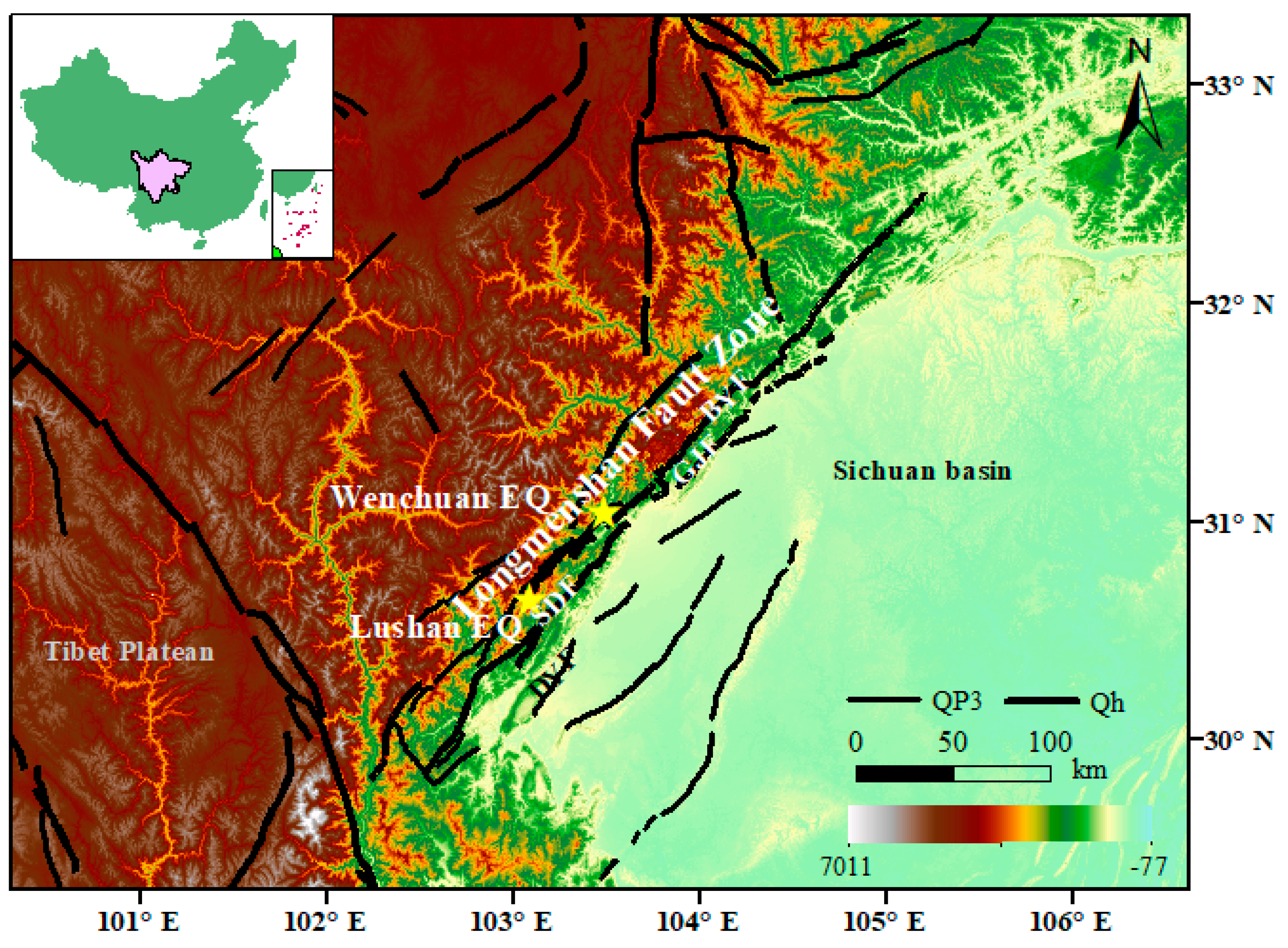
Abstract
:1. Introduction
2. Tectonic Setting
3. Materials and Methods
3.1. Climatological Data
3.2. Analysis Method

4. Result
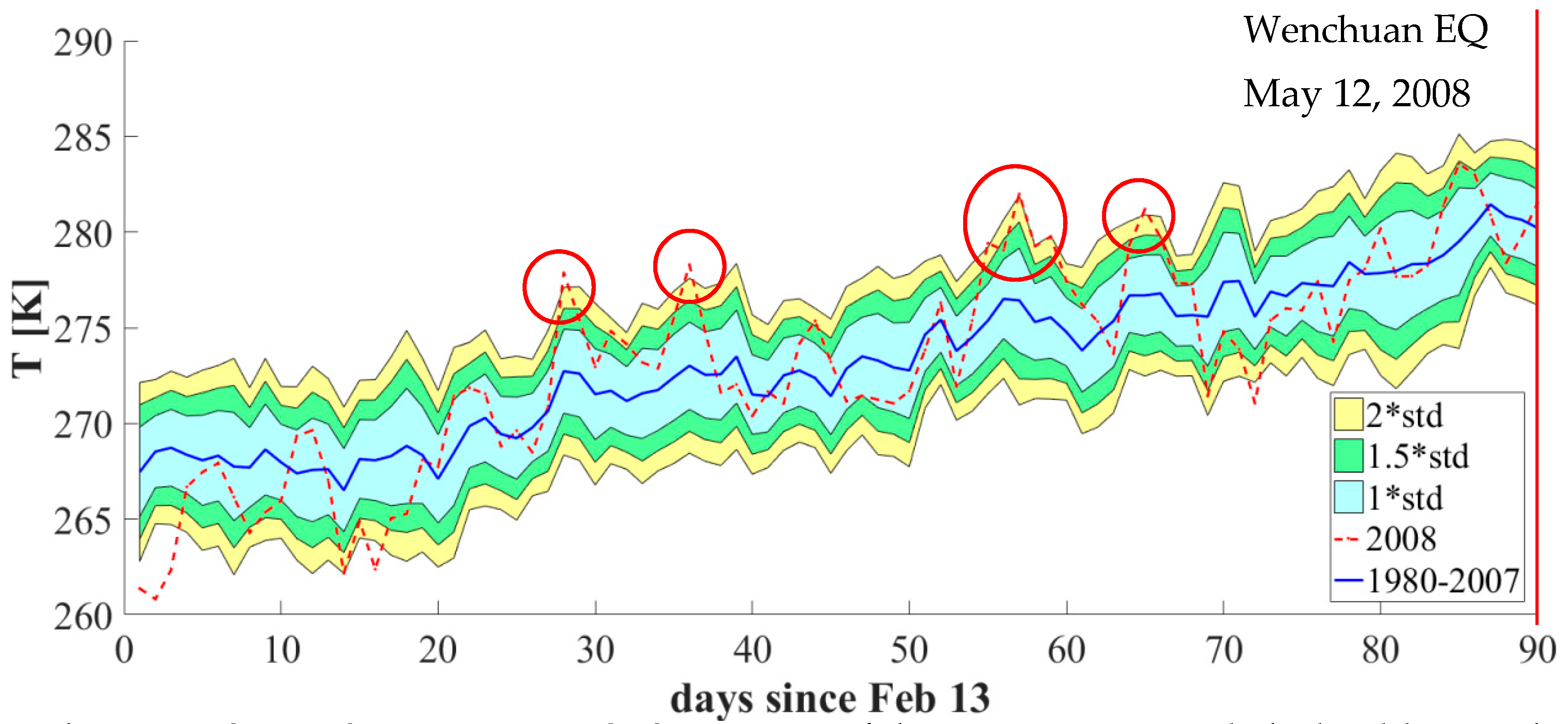
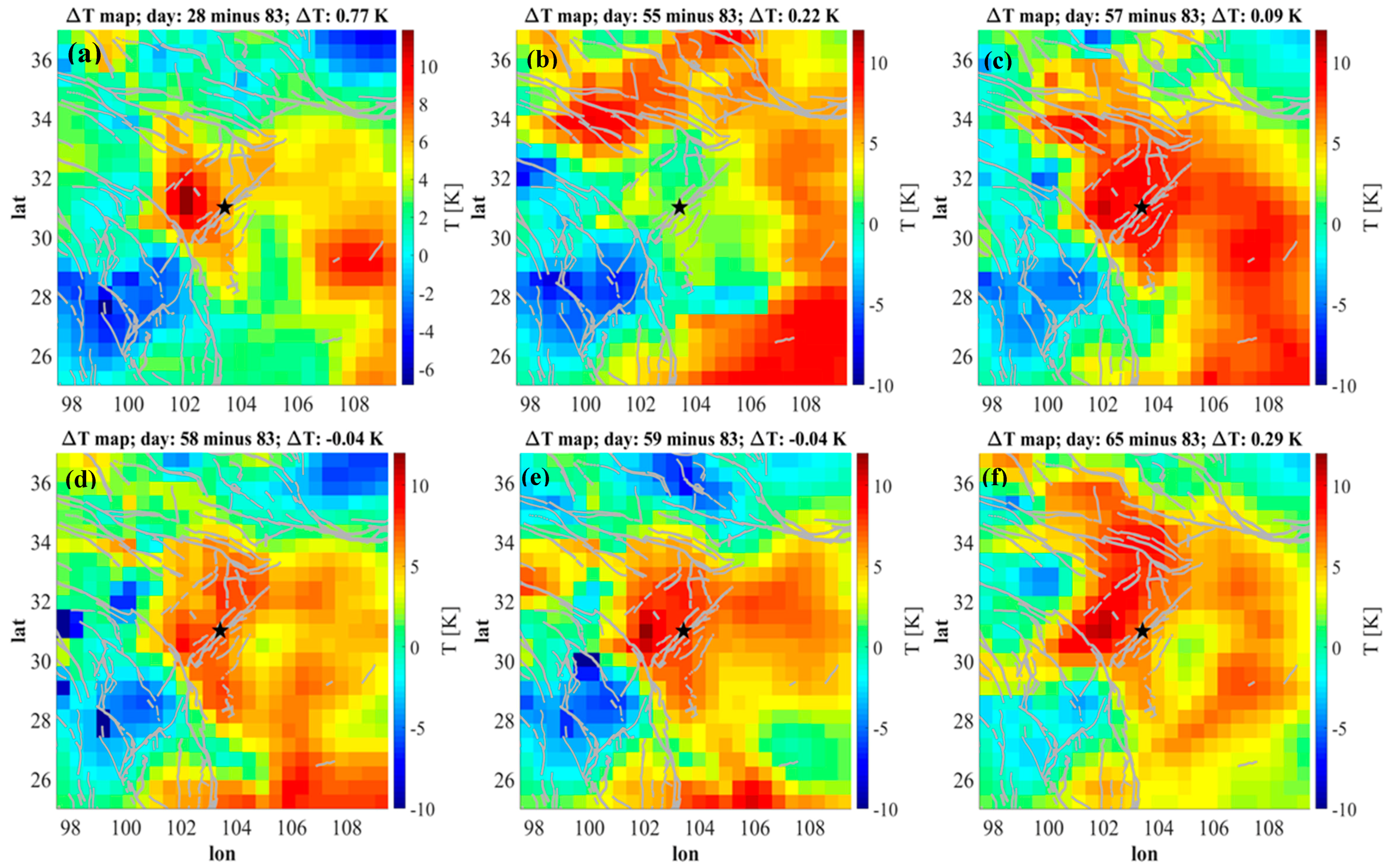
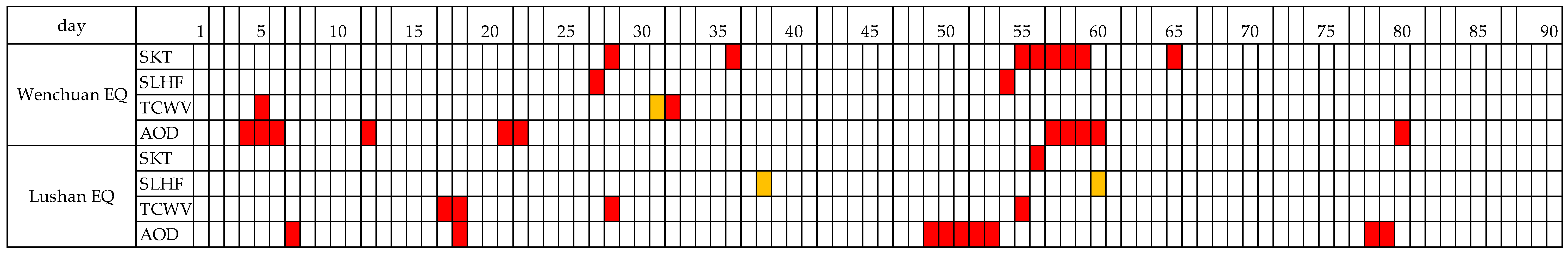
4.1. Case Study: Wenchuan EQ
4.1.1. SKT
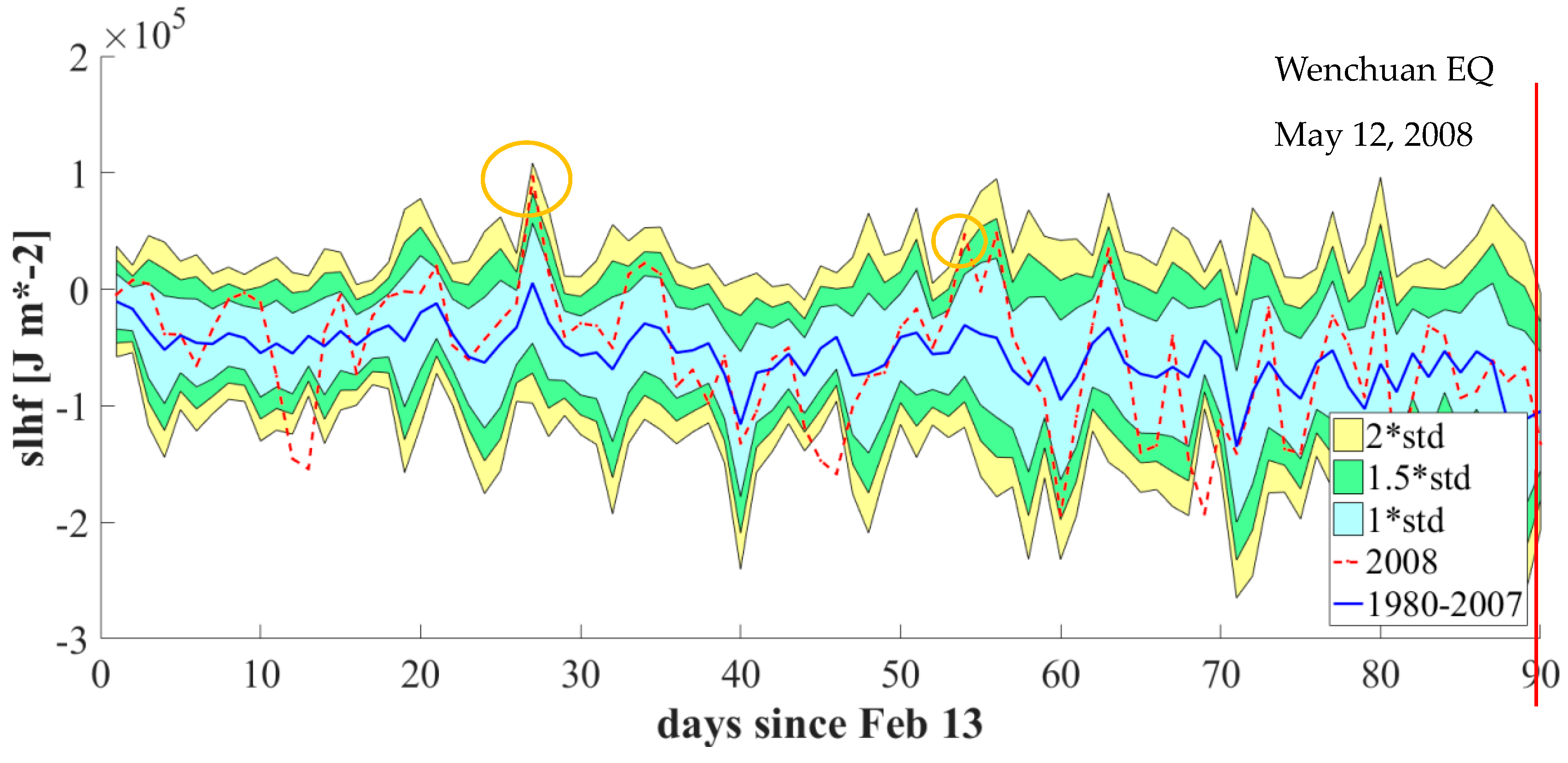
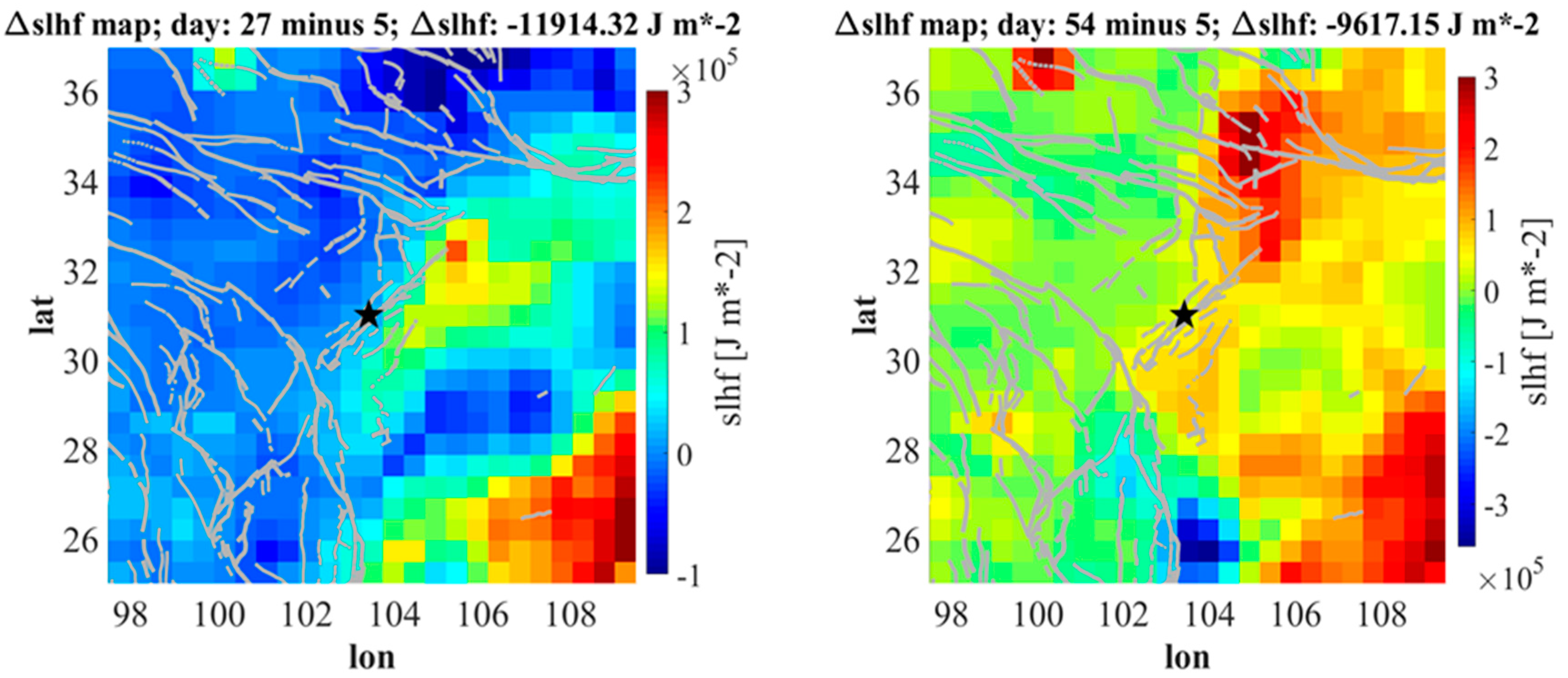
4.1.2. SLHF
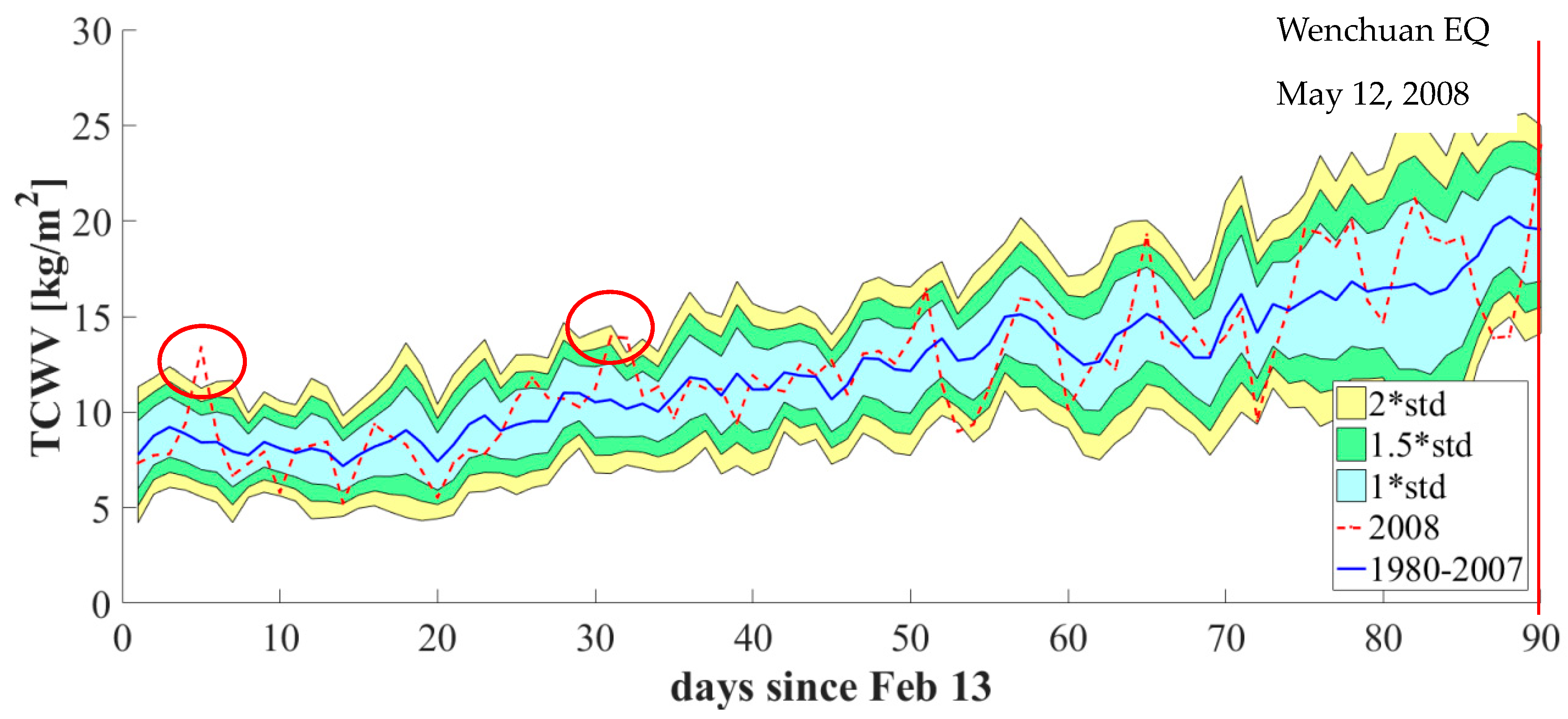
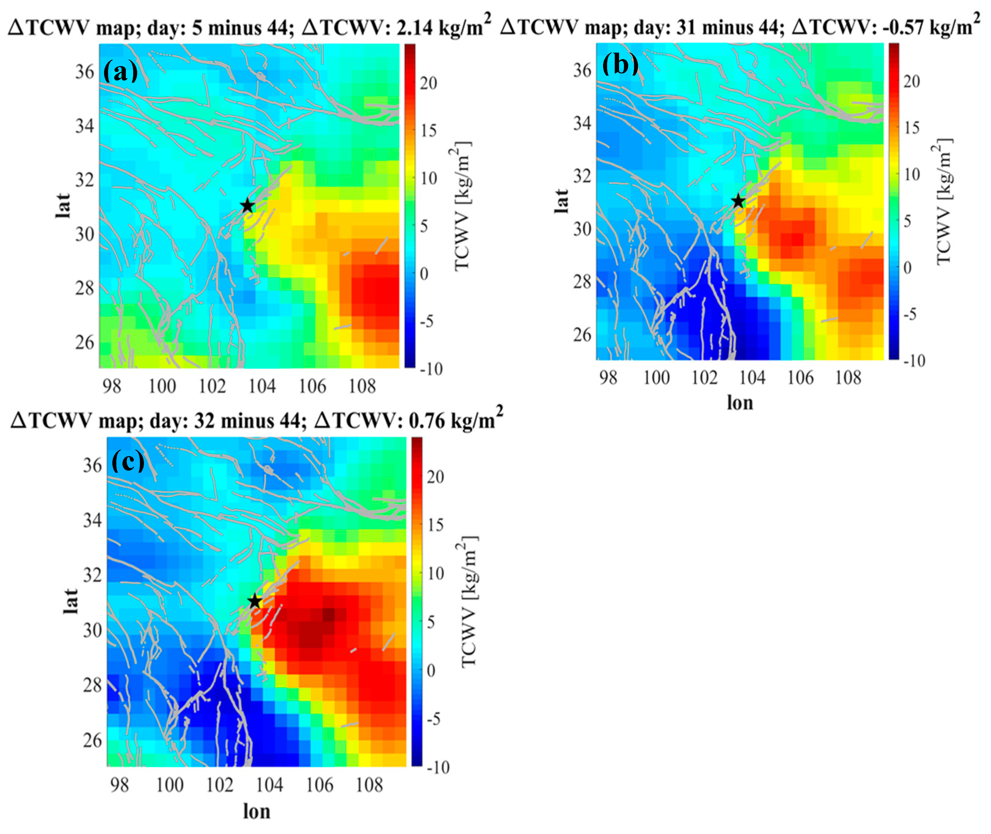
4.1.3. TCWV
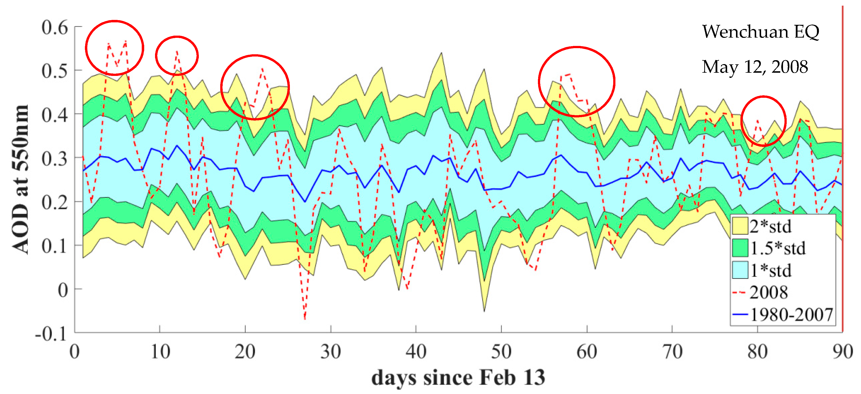
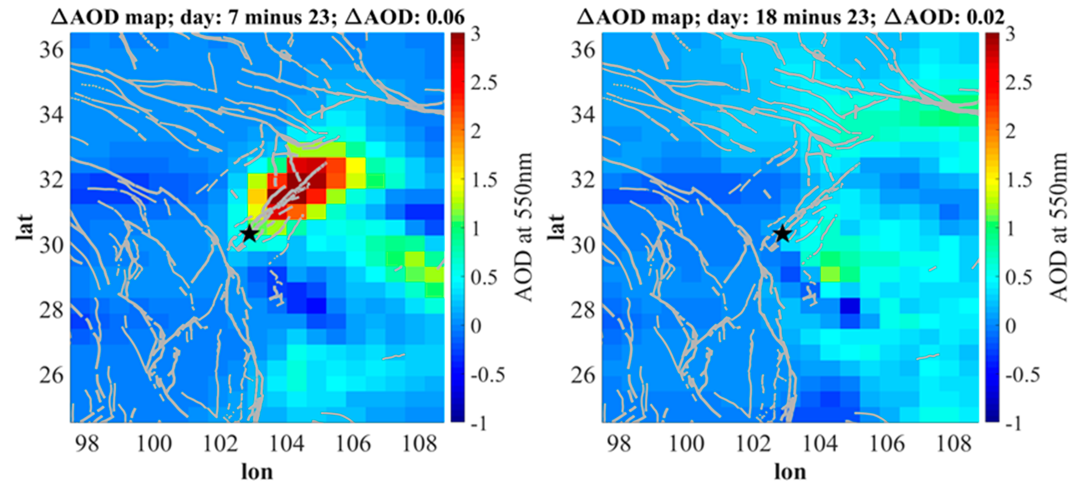
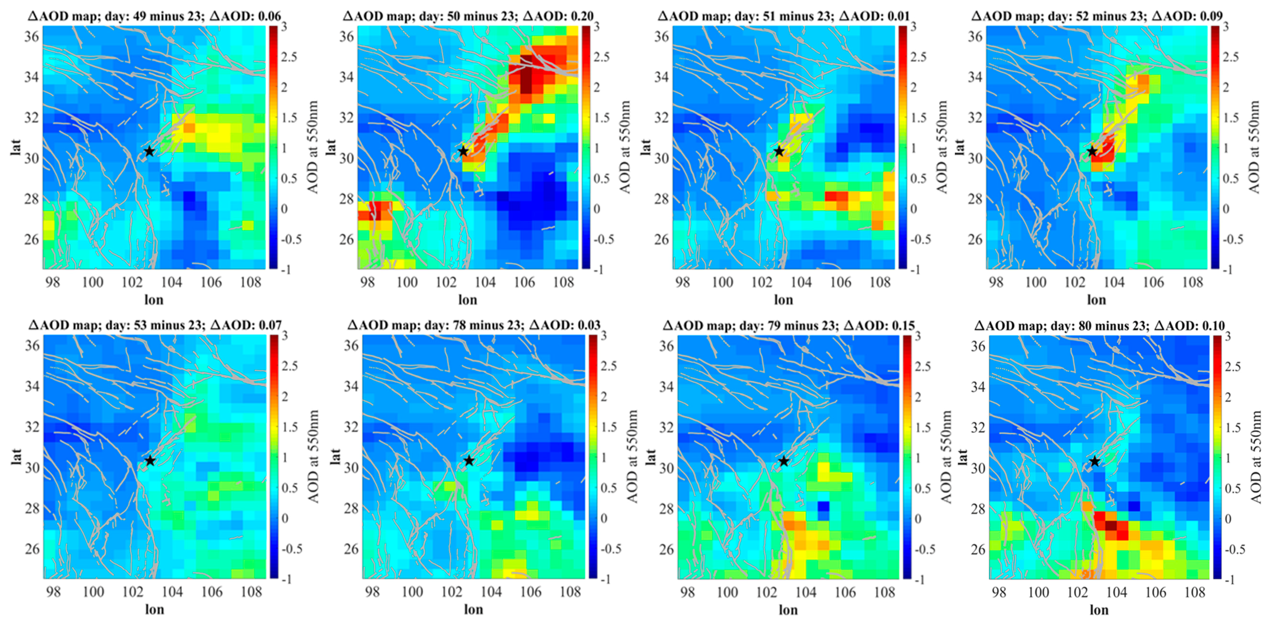
4.1.4. AOD
4.2. Case Study: Lushan EQ
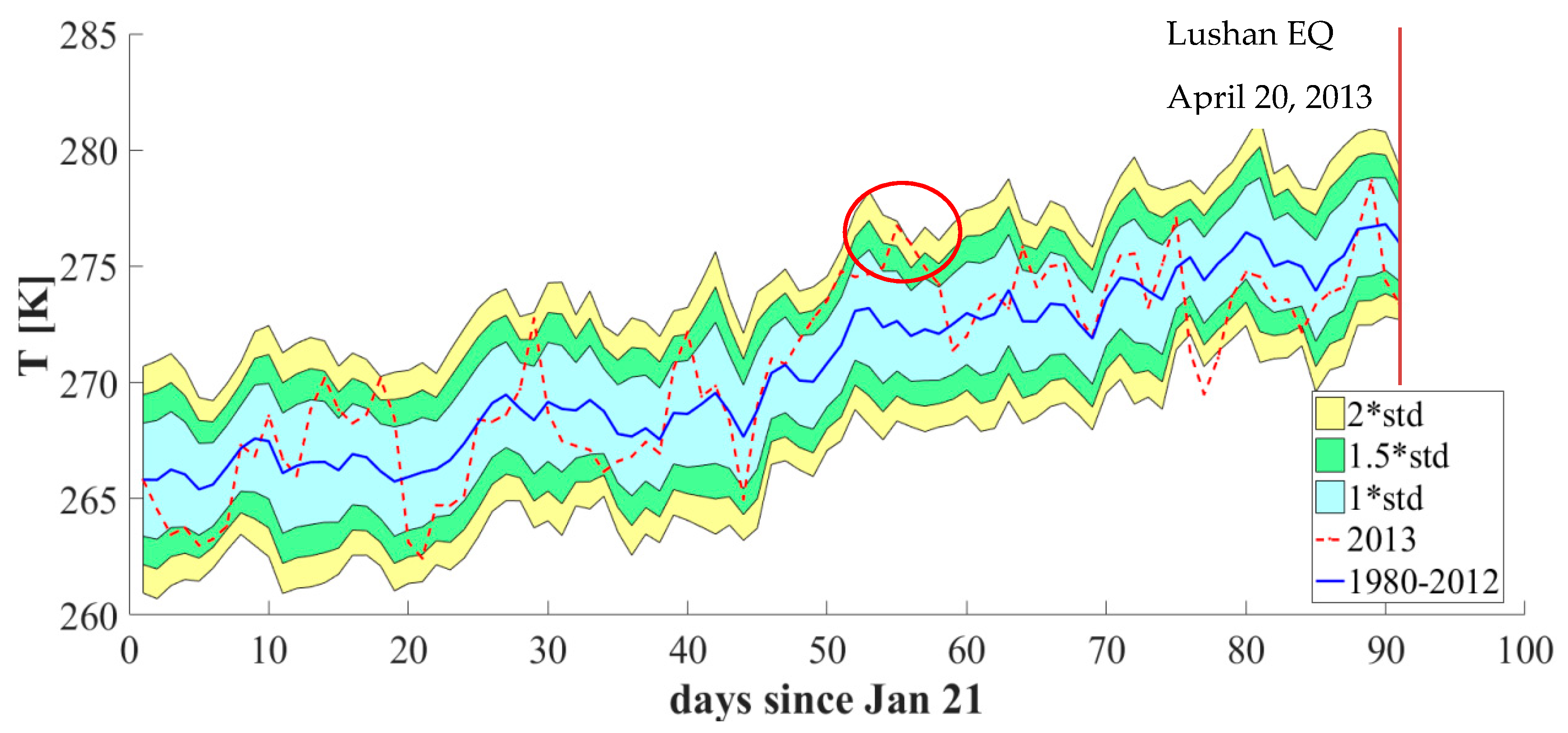
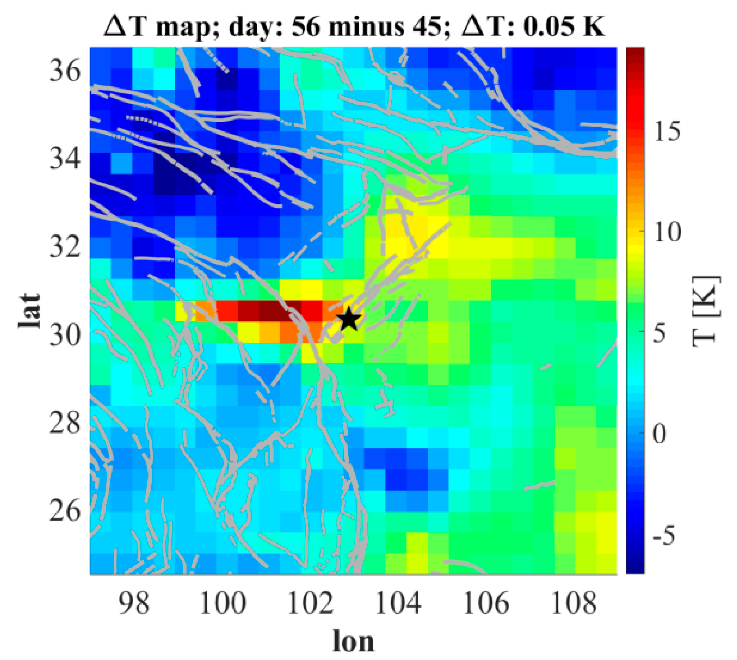
4.2.1. SKT
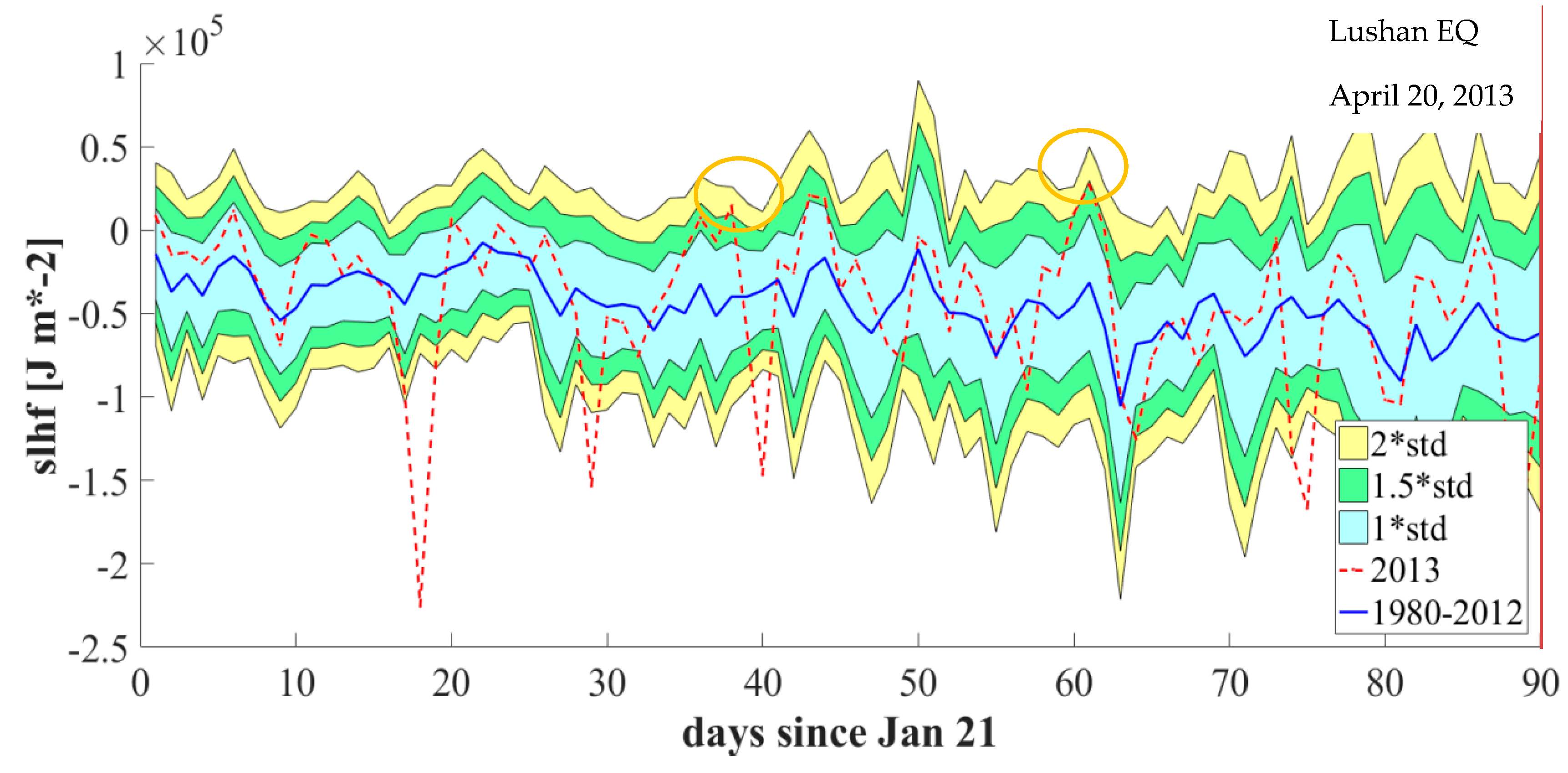
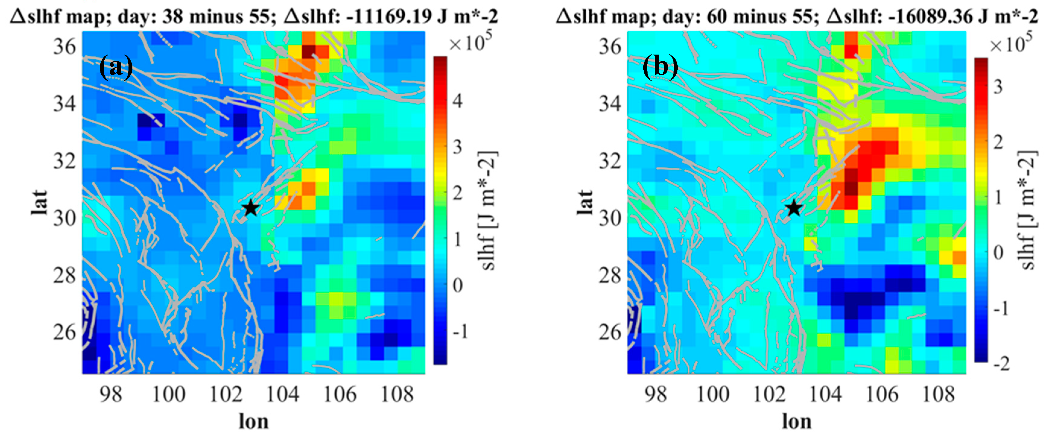
4.2.2. SLHF
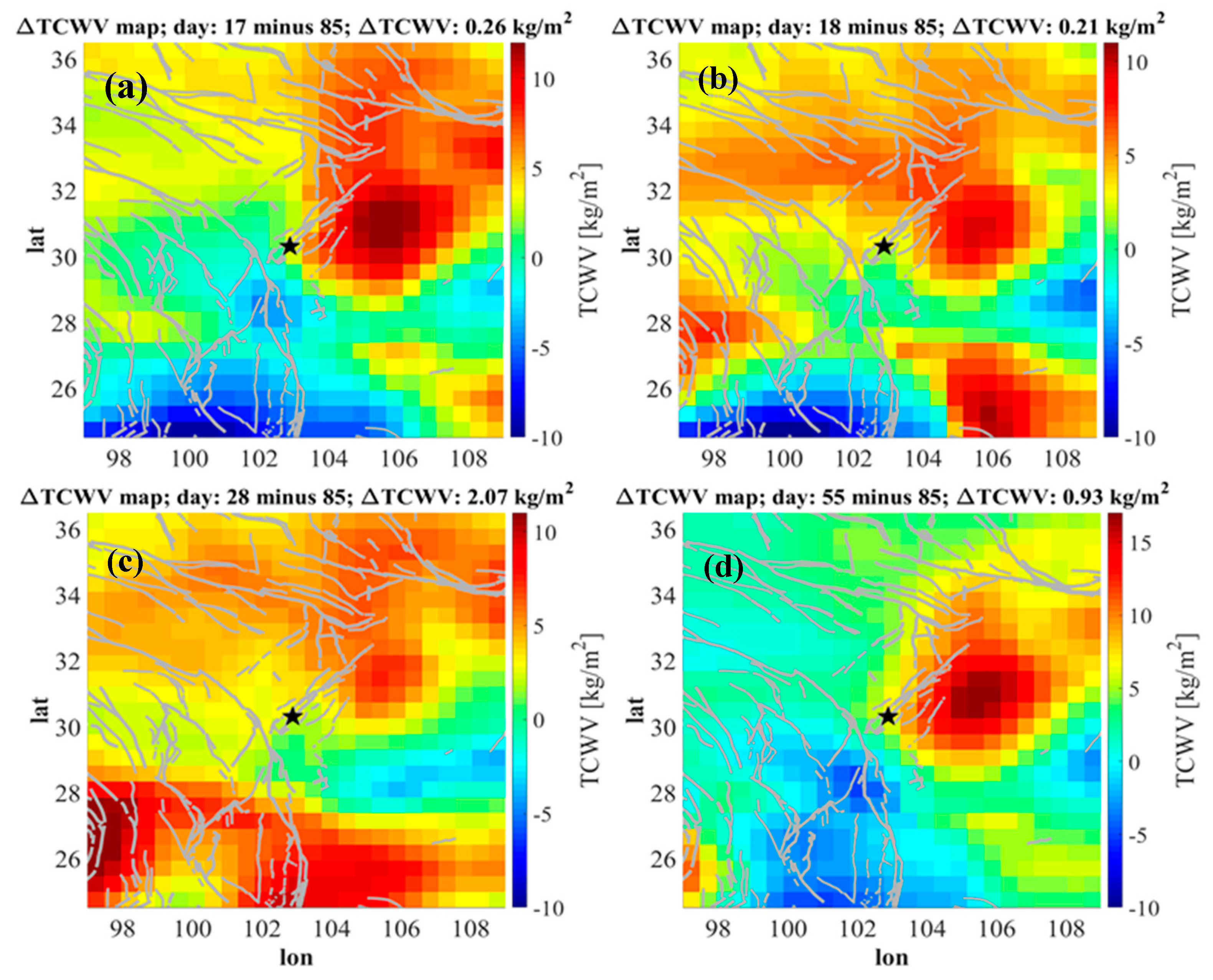
4.2.3. TCWV
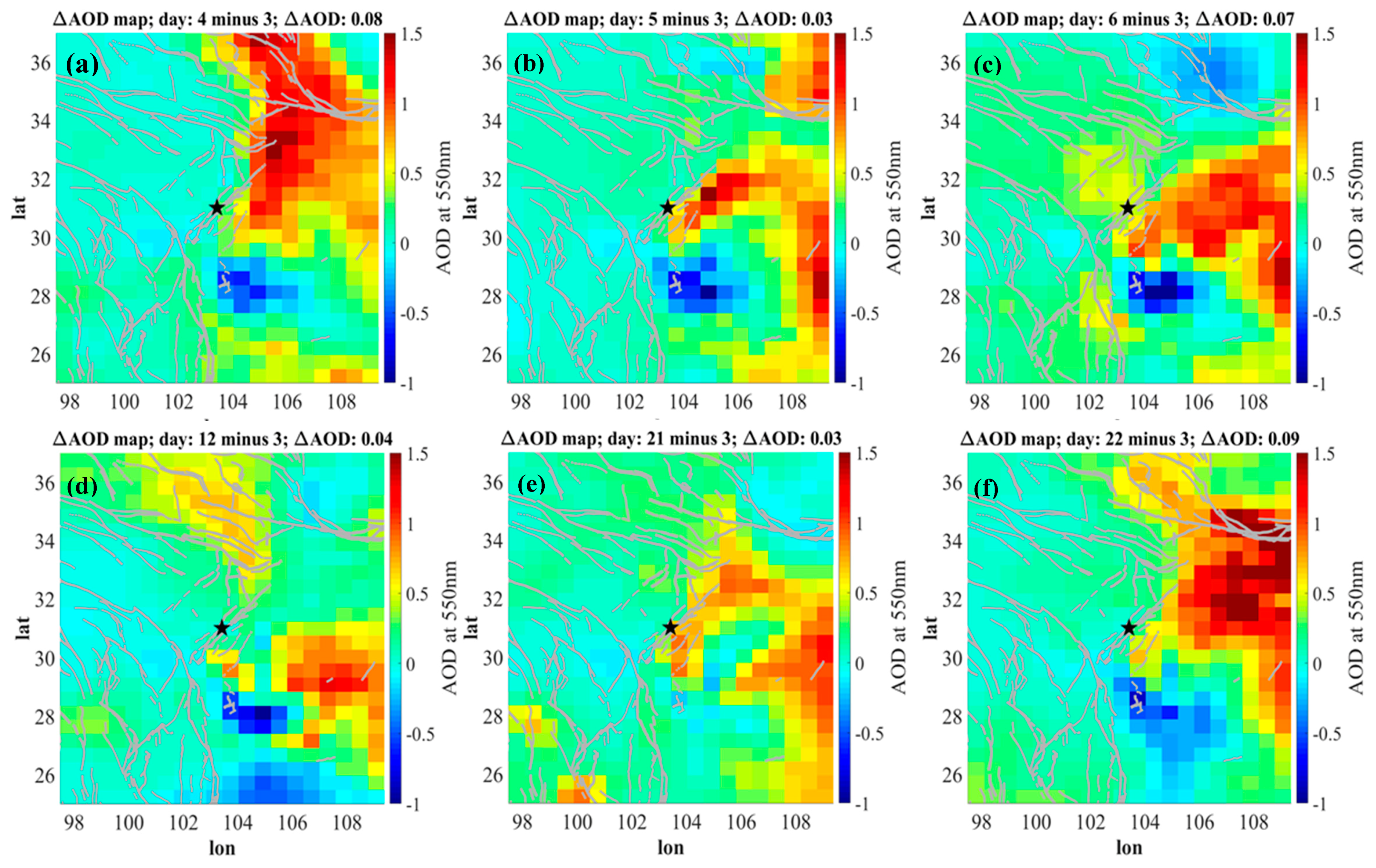
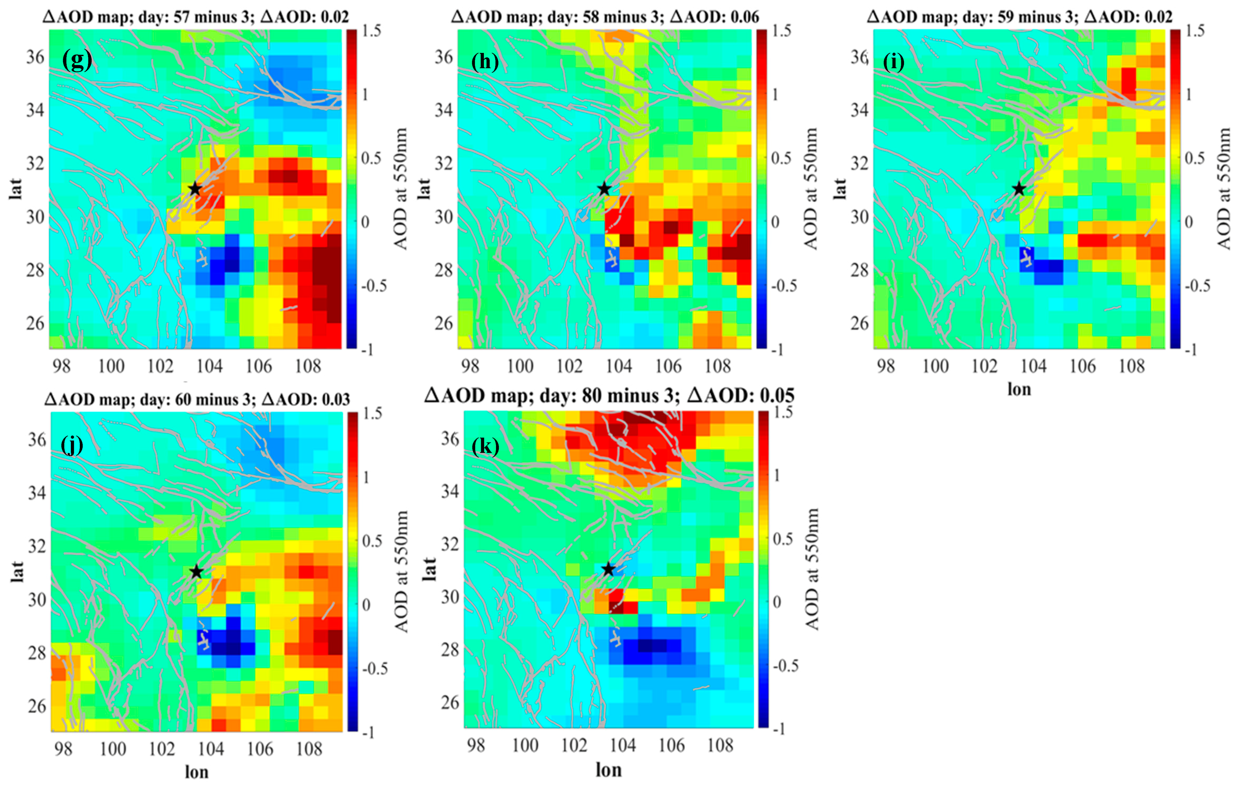
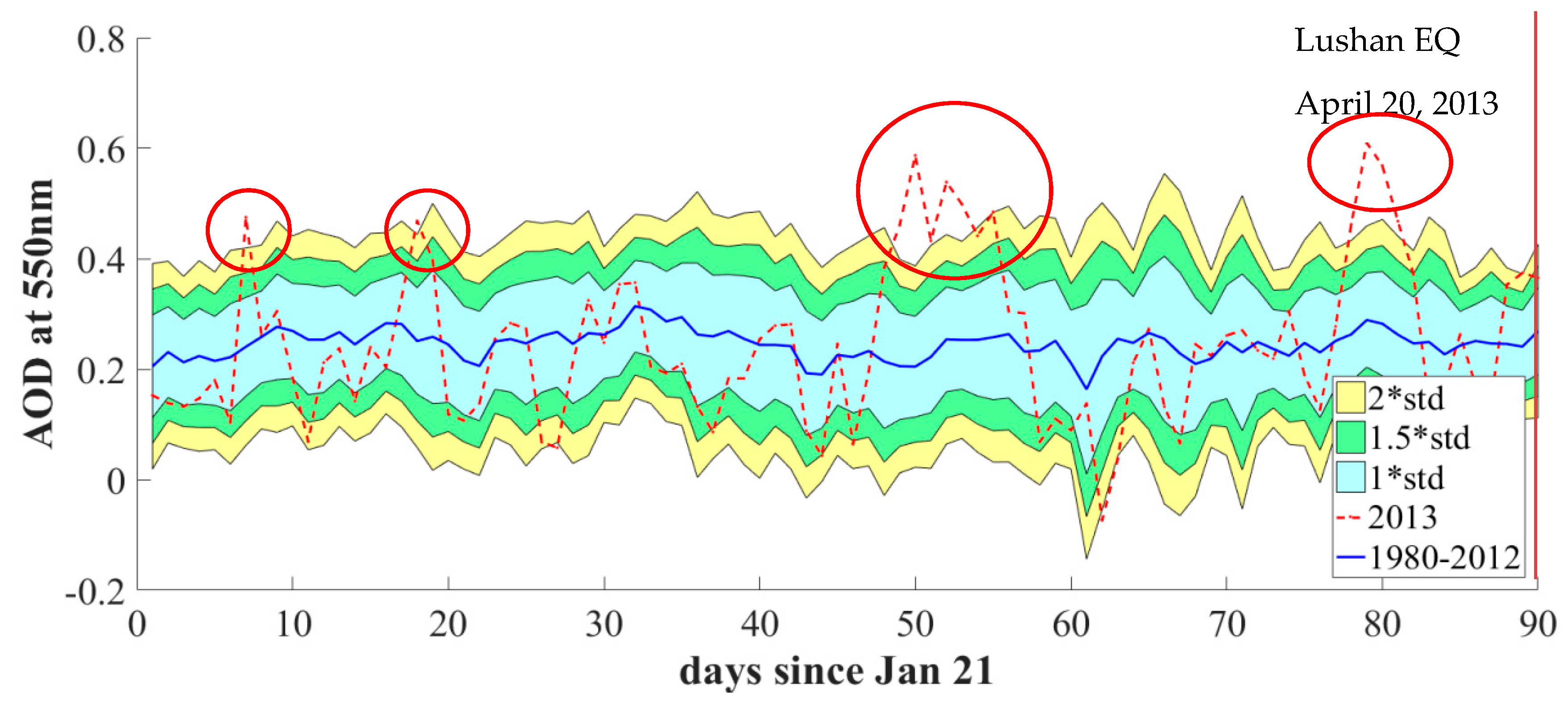
4.2.4. AOD
5. Discussion
6. Conclusions
Supplementary Materials
Supplementary File 1Author Contributions
Funding
Acknowledgments
Conflicts of Interest
References
- Tronin, A. Satellite Remote Sensing in Seismology. A Review. Remote Sens.-Basel 2010, 2, 124–150. [Google Scholar] [CrossRef] [Green Version]
- Carlson, J.M.; Langer, J.S. Mechanical model of an earthquake fault. Phys. Rev. A. 1989, 40, 6470–6484. [Google Scholar] [CrossRef] [PubMed] [Green Version]
- Bizzarri, A. What Does Control Earthquake Ruptures and Dynamic Faulting? A Review of Different Competing Mechanisms. Pure Appl. Geophys. 2009, 166, 741–776. [Google Scholar] [CrossRef]
- Miller, S.A. Chapter 1—The Role of Fluids in Tectonic and Earthquake Processes. In Advances in Geophysics; Dmowska, R., Ed.; Elsevier: Amsterdam, The Netherlands, 2013; Volume 54, pp. 1–46. [Google Scholar]
- Dobrovolsky, I.P.; Zubkov, S.I.; Miachkin, V.I. Estimation of the size of earthquake preparation zones. Pure Appl. Geophys. 1979, 117, 1025–1044. [Google Scholar] [CrossRef]
- Sobolev, G.A.; Huang, Q.; Nagao, T. Phases of earthquake’s preparation and by chance test of seismic quiescence anomaly. J. Geodyn. 2002, 33, 413–424. [Google Scholar] [CrossRef]
- Pulinets, S.; Ouzounov, D. Lithosphere–Atmosphere–Ionosphere Coupling (LAIC) model—An unified concept for earthquake precursors validation. J. Asian Earth Sci. 2011, 41, 371–382. [Google Scholar] [CrossRef]
- Roeloffs, E.A. Evidence for aseismic deformation rate changes prior to earthquakes. Annu. Rev. Earth Planet. Sci. 2006, 34, 591–627. [Google Scholar] [CrossRef] [Green Version]
- Cicerone, R.D.; Ebel, J.E.; Britton, J. A systematic compilation of earthquake precursors. Tectonophysics 2009, 476, 371–396. [Google Scholar] [CrossRef]
- Tramutoli, V.; Aliano, C.; Corrado, R.; Filizzola, C.; Genzano, N.; Lisi, M.; Martinelli, G.; Pergola, N. On the possible origin of thermal infrared radiation (TIR) anomalies in earthquake-prone areas observed using robust satellite techniques (RST). Chem. Geol. 2013, 339, 157–168. [Google Scholar] [CrossRef]
- Qin, K.; Wu, L.; Zheng, S.; Liu, S. A Deviation-Time-Space-Thermal (DTS-T) Method for Global Earth Observation System of Systems (GEOSS)-Based Earthquake Anomaly Recognition: Criterions and Quantify Indices. Remote Sens. Basel. 2013, 5, 5143–5151. [Google Scholar] [CrossRef] [Green Version]
- Dey, S.; Singh, R.P. Surface latent heat flux as an earthquake precursor. Nat. Hazards Earth Syst. Sci. 2003, 3, 749–755. [Google Scholar] [CrossRef]
- Xiong, P.; Shen, X.H.; Bi, Y.X.; Kang, C.L.; Chen, L.Z.; Jing, F.; Chen, Y. Study of outgoing longwave radiation anomalies associated with Haiti earthquake. Nat. Hazards Earth Syst. Sci. 2010, 10, 2169–2178. [Google Scholar] [CrossRef] [Green Version]
- Ganguly, N.D. Atmospheric changes observed during April 2015 Nepal earthquake. J. Atmos. Sol. Terr. Phys. 2016, 140, 16–22. [Google Scholar] [CrossRef]
- Akhoondzadeh, M.; De Santis, A.; Marchetti, D.; Piscini, A.; Cianchini, G. Multi precursors analysis associated with the powerful Ecuador (MW=7.8) earthquake of 16 April 2016 using Swarm satellites data in conjunction with other multi-platform satellite and ground data. Adv. Space Res. 2018, 61, 248–263. [Google Scholar] [CrossRef] [Green Version]
- Qin, K.; Wu, L.X.; Zheng, S.; Bai, Y.; Lv, X. Is there an abnormal enhancement of atmospheric aerosol before the 2008 Wenchuan earthquake? Adv. Space Res. 2014, 54, 1029–1034. [Google Scholar] [CrossRef]
- Akhoondzadeh, M.; De Santis, A.; Marchetti, D.; Piscini, A.; Jin, S. Anomalous seismo-LAI variations potentially associated with the 2017 Mw = 7.3 Sarpol-e Zahab (Iran) earthquake from Swarm satellites, GPS-TEC and climatological data. Adv. Space Res. 2019, 64, 143–158. [Google Scholar] [CrossRef]
- Li, C.; Wei, Z.; Ye, J.; Han, Y.; Zheng, W. Amounts and styles of coseismic deformation along the northern segment of surface rupture, of the 2008 Wenchuan Mw 7.9 earthquake, China. Tectonophysics 2010, 491, 35–58. [Google Scholar] [CrossRef]
- Liu-Zeng, J.; Zhang, Z.; Wen, L.; Tapponnier, P.; Sun, J.; Xing, X.; Hu, G.; Xu, Q.; Zeng, L.; Ding, L.; et al. Co-seismic ruptures of the 12 May 2008, Ms 8.0 Wenchuan earthquake, Sichuan: East–west crustal shortening on oblique, parallel thrusts along the eastern edge of Tibet. Earth Planet. Sci. Lett. 2009, 286, 355–370. [Google Scholar] [CrossRef]
- Chen, Q.; Liu, X.; Zhang, Y.; Zhao, J.; Xu, Q.; Yang, Y.; Liu, G. A nonlinear inversion of InSAR-observed coseismic surface deformation for estimating variable fault dips in the 2008 Wenchuan earthquake. Int. J. Appl. Earth Obs. 2019, 76, 179–192. [Google Scholar] [CrossRef]
- Dong, S.; Han, Z.; An, Y. Paleoseismological events in the “seismic gap” between the 2008 Wenchuan and the 2013 Lushan earthquakes and implications for future seismic potential. J. Asian Earth Sci. 2017, 135, 1–15. [Google Scholar] [CrossRef]
- Li, Z.; Wen, Y.; Zhang, P.; Liu, Y.; Zhang, Y. Joint Inversion of GPS, Leveling, and InSAR Data for The 2013 Lushan (China) Earthquake and Its Seismic Hazard Implications. Remote Sens. Basel. 2020, 12, 715. [Google Scholar] [CrossRef] [Green Version]
- Chen, L.; Ran, Y.; Wang, H.; Li, Y.; Ma, X. The Lushan M S7.0 earthquake and activity of the southern segment of the LMSF zone. Chin. Sci. Bull. 2013, 58, 3475–3482. [Google Scholar] [CrossRef] [Green Version]
- Fang, L.; Wu, J.; Wang, W.; Lü, Z.; Wang, C.; Yang, T.; Cai, Y. Relocation of the mainshock and aftershock sequences of M S7.0 Sichuan Lushan earthquake. Chin. Sci. Bull. 2013, 58, 3451–3459. [Google Scholar] [CrossRef] [Green Version]
- Li, Y.; Jia, D.; Wang, M.; Shaw, J.H.; He, J.; Lin, A.; Xiong, L.; Rao, G. Structural geometry of the source region for the 2013 Mw 6.6 Lushan earthquake: Implication for earthquake hazard assessment along the Longmen Shan. Earth Planet. Sci. Lett. 2014, 390, 275–286. [Google Scholar] [CrossRef]
- Piscini, A.; De Santis, A.; Marchetti, D.; Cianchini, G. A Multi-parametric Climatological Approach to Study the 2016 Amatrice–Norcia (Central Italy) Earthquake Preparatory Phase. Pure Appl. Geophys. 2017, 174, 3673–3688. [Google Scholar] [CrossRef]
- De Santis, A.; Abbattista, C.; Alfonsi, L.; Amoruso, L.; Campuzano, S.A.; Carbone, M.; Cesaroni, C.; Cianchini, G.; De Franceschi, G.; Di Giovambattista, R.; et al. Geosystemics view of Earthquakes. Entropy 2019, 21, 412. [Google Scholar] [CrossRef] [Green Version]
- Zhang, P.; Wen, X.; Shen, Z.; Chen, J. Oblique, High-Angle, Listric-Reverse Faulting and Associated Development of Strain: The Wenchuan Earthquake of May 12, 2008, Sichuan, China. Annu. Rev. Earth Planet. Sci. 2010, 38, 353–382. [Google Scholar] [CrossRef] [Green Version]
- Xu, X.; Wen, X.; Han, Z.; Chen, G.; Li, C.; Zheng, W.; Zhnag, S.; Ren, Z.; Xu, C.; Tan, X.; et al. Lushan M S7.0 earthquake: A blind reserve-fault event. Chin. Sci. Bull 2013, 58, 3437–3443. [Google Scholar] [CrossRef] [Green Version]
- Liang, W.; Zhao, Y.; Xu, Y.; Zhu, Y.; Guo, S.; Liu, F.; Liu, L. Gravity observations along the eastern margin of the Tibetan Plateau and an application to the Lushan MS7.0 earthquake. Earthq. Sci. 2013, 26, 251–257. [Google Scholar] [CrossRef] [Green Version]
- Wang, Z.; Su, J.; Liu, C.; Cai, X. New insights into the generation of the 2013 Lushan Earthquake (Ms 7.0), China. J. Geophys. Res. Solid Earth 2015, 120, 3507–3526. [Google Scholar] [CrossRef]
- Wang, Z.; Fukao, Y.; Pei, S. Structural control of rupturing of the Mw7.9 2008 Wenchuan Earthquake, China. Earth Planet. Sci. Lett. 2009, 279, 131–138. [Google Scholar] [CrossRef]
- Wei, W.; Unsworth, M.; Jones, A.; Booker, J.; Tan, H.; Nelson, D.; Chen, L.; Li, S.; Solon, K.; Bedrosian, P.; et al. Detection of Widespread Fluids in the Tibetan Crust by Magnetotelluric Studies. Science 2001, 292, 716. [Google Scholar] [CrossRef] [PubMed]
- Zhao, G.; Unsworth, M.J.; Zhan, Y.; Wang, L.; Chen, X.; Jones, A.G.; Tang, J.; Xiao, Q.; Wang, J.; Cai, J.; et al. Crustal structure and rheology of the Longmenshan and Wenchuan Mw 7.9 earthquake epicentral area from magnetotelluric data. Geology 2012, 40, 1139–1142. [Google Scholar] [CrossRef]
- Lei, J.; Zhao, D. Structural heterogeneity of the LMSF zone and the mechanism of the 2008 Wenchuan earthquake (Ms 8.0). Geochem. Geophys. Geosys. 2009, 10, 10. [Google Scholar] [CrossRef]
- Cui, Y.; Ouzounov, D.; Hatzopoulos, N.; Sun, K.; Zou, Z.; Du, J. Satellite observation of CH4 and CO anomalies associated with the Wenchuan MS 8.0 and Lushan MS 7.0 earthquakes in China. Chem. Geol. 2017, 469, 185–191. [Google Scholar] [CrossRef] [Green Version]
- Piscini, A.; Marchetti, D.; De Santis, A. Multi-Parametric Climatological Analysis Associated with Global Significant Volcanic Eruptions During 2002–2017. Pure Appl. Geophys. 2019, 176, 3629–3647. [Google Scholar] [CrossRef]
- Manney, G.L.; Hegglin, M.I.; Lawrence, Z.D.; Wargan, K.; Millán, L.F.; Schwartz, M.J.; Santee, M.L.; Lambert, A.; Pawson, S.; Knosp, B.W.; et al. Reanalysis comparisons of upper tropospheric–lower stratospheric jets and multiple tropopauses. Atmos. Chem. Phys. 2017, 17, 11541–11566. [Google Scholar] [CrossRef] [Green Version]
- Chen, Q.F.; Wang, K. The 2008 Wenchuan Earthquake and Earthquake Prediction in China. Bull. Seismol. Soc. Am. 2010, 100, 2840–2857. [Google Scholar] [CrossRef]
- Wu, J.; Yao, D.; Meng, X.; Peng, Z.; Su, J.; Long, F. Spatial-temporal evolutions of early aftershocks following the 2013 Mw6.6 Lushan earthquake in Sichuan, China. J. Geophys. Res. Solid Earth 2017, 122, 2873–2889. [Google Scholar] [CrossRef]
- Wang, X.; Zhang, G.; Fang, H.; Luo, W.; Zhang, W.; Zhong, Q.; Cai, X.; Luo, H. Crust and upper mantle resistivity structure at middle section of Longmenshan, eastern Tibetan plateau. Tectonophysics 2014, 619-620, 143–148. [Google Scholar] [CrossRef]
- Cui, J.; Shen, X.; Zhang, J.; Ma, W.; Chu, W. Analysis of spatiotemporal variations in middle-tropospheric to upper-tropospheric methane during the Wenchuan Ms=8.0 earthquake by three indices. Nat. Hazard. Earth Syst. Sci. 2019, 19, 2841–2854. [Google Scholar] [CrossRef] [Green Version]
- Ye, Q.; Singh, R.P.; He, A.; Ji, S.; Liu, C. Characteristic behavior of water radon associated with Wenchuan and Lushan earthquakes along LMSF. Radiat. Meas. 2015, 76, 44–53. [Google Scholar] [CrossRef]
- Shen, X.H.; Zhang, X.; Hong, S.; Jing, F.; Zhao, S. Progress and development on multi-parameters remote sensing application in earthquake monitoring in China. Earthq. Sci. 2013, 26, 427–437. [Google Scholar] [CrossRef] [Green Version]
- Liu, Q.Q.; Shen, X.H.; Zhang, J.; Li, M. Exploring the abnormal fluctuations of atmospheric aerosols before the 2008 Wenchuan and 2013 Lushan earthquakes. Adv. Space Res. 2019, 63, 3768–3776. [Google Scholar] [CrossRef]
- Dey, S.; Sarkar, S.; Singh, R.P. Anomalous changes in column water vapor after Gujarat earthquake. Adv. Space Res. 2004, 33, 274–278. [Google Scholar] [CrossRef]
- Boncio, P. Deep-crust strike-slip earthquake faulting in southern Italy aided by high fluid pressure: Insights from rheological analysis. Geol. Soc. Lond. Spec. Publ. 2008, 299, 195–210. [Google Scholar] [CrossRef] [Green Version]
- Cappa, F.; Rutqvist, J.; Yamamoto, K. Modeling crustal deformation and rupture processes related to upwelling of deep CO2-rich fluids during the 1965–1967 Matsushiro earthquake swarm in Japan. J. Geophys. Res. 2009, 114. [Google Scholar] [CrossRef] [Green Version]
- Miller, S.A.; Collettini, C.; Chiaraluce, L.; Cocco, M.; Barchi, M.; Kaus, B.J.P. Aftershocks driven by a high-pressure CO2 source at depth. Nature 2004, 427, 724–727. [Google Scholar] [CrossRef]
- Di Luccio, F.; Ventura, G.; Di Giovambattista, R.; Piscini, A.; Cinti, F.R. Normal faults and thrusts reactivated by deep fluids: The 6 April 2009 Mw 6.3 L’Aquila earthquake, central Italy. J. Geophys. Res. 2010, 115. [Google Scholar] [CrossRef]
- Cianchini, G.; De Santis, A.; Barraclough, D.R.; Wu, L.X.; Qin, K. Magnetic transfer function entropy and the 2009 Mw = 6.3 L’Aquila earthquake (Central Italy). Nonlinear Proc. Geoph. 2012, 19, 401–409. [Google Scholar] [CrossRef] [Green Version]
- Burchfiel, B.C.; Royden, L.H.; van der Hilst, R.D.; Hager, B.H.; Chen, Z.; King, R.W.; Li, C.; Lü, J.; Yao, H.; Kirby, E. A geological and geophysical context for the Wenchuan earthquake of 12 May 2008, Sichuan, People’s Republic of China. GSA Today 2008, 18, 4. [Google Scholar] [CrossRef]
- Xie, T.; Ma, W. Possible thermal brightness temperature anomalies associated with the Lushan (China) M S7.0 earthquake on 20 April 2013. Earthq. Sci. 2015, 28, 37–47. [Google Scholar] [CrossRef] [Green Version]
- Li, Y.; Zhang, G.; Shan, X.; Liu, Y.; Wu, Y.; Liang, H.; Qu, C.; Song, X. GPS-Derived Fault Coupling of the Longmenshan Fault Associated with the 2008 Mw Wenchuan 7.9 Earthquake and Its Tectonic Implications. Remote Sens. Basel. 2018, 10, 753. [Google Scholar] [CrossRef] [Green Version]


© 2020 by the authors. Licensee MDPI, Basel, Switzerland. This article is an open access article distributed under the terms and conditions of the Creative Commons Attribution (CC BY) license (http://creativecommons.org/licenses/by/4.0/).
Share and Cite
Liu, Q.; De Santis, A.; Piscini, A.; Cianchini, G.; Ventura, G.; Shen, X. Multi-Parametric Climatological Analysis Reveals the Involvement of Fluids in the Preparation Phase of the 2008 Ms 8.0 Wenchuan and 2013 Ms 7.0 Lushan Earthquakes. Remote Sens. 2020, 12, 1663. https://0-doi-org.brum.beds.ac.uk/10.3390/rs12101663
Liu Q, De Santis A, Piscini A, Cianchini G, Ventura G, Shen X. Multi-Parametric Climatological Analysis Reveals the Involvement of Fluids in the Preparation Phase of the 2008 Ms 8.0 Wenchuan and 2013 Ms 7.0 Lushan Earthquakes. Remote Sensing. 2020; 12(10):1663. https://0-doi-org.brum.beds.ac.uk/10.3390/rs12101663
Chicago/Turabian StyleLiu, Qinqin, Angelo De Santis, Alessandro Piscini, Gianfranco Cianchini, Guido Ventura, and Xuhui Shen. 2020. "Multi-Parametric Climatological Analysis Reveals the Involvement of Fluids in the Preparation Phase of the 2008 Ms 8.0 Wenchuan and 2013 Ms 7.0 Lushan Earthquakes" Remote Sensing 12, no. 10: 1663. https://0-doi-org.brum.beds.ac.uk/10.3390/rs12101663