Hyperspectral Image Classification Based on a Shuffled Group Convolutional Neural Network with Transfer Learning

Abstract

Convolutional neural networks (CNNs) have been widely applied in hyperspectral imagery (HSI) classification. However, their classification performance might be limited by the scarcity of labeled data to be used for training and validation. In this paper, we propose a novel lightweight shuffled group convolutional neural network (abbreviated as SG-CNN) to achieve efficient training with a limited training dataset in HSI classification. SG-CNN consists of SG conv units that employ conventional and atrous convolution in different groups, followed by channel shuffle operation and shortcut connection. In this way, SG-CNNs have less trainable parameters, whilst they can still be accurately and efficiently trained with fewer labeled samples. Transfer learning between different HSI datasets is also applied on the SG-CNN to further improve the classification accuracy. To evaluate the effectiveness of SG-CNNs for HSI classification, experiments have been conducted on three public HSI datasets pretrained on HSIs from different sensors. SG-CNNs with different levels of complexity were tested, and their classification results were compared with fine-tuned ShuffleNet2, ResNeXt, and their original counterparts. The experimental results demonstrate that SG-CNNs can achieve competitive classification performance when the amount of labeled data for training is poor, as well as efficiently providing satisfying classification results.

1. Introduction

Hyperspectral sensors are able to grasp detailed information of objects and phenomena on Earth’s surface by severing their spectral characteristics in a large number of channels (bands) over a wide portion of the electromagnetic spectrum. Such rich spectral information allows hyperspectral imagery (HSI) to be used for interpretation and analysis of surface materials in a more thorough way. Accordingly, hyperspectral remote sensing has been widely used in several research fields, such as environmental monitoring [1,2,3], land management [4,5,6], and agriculture [7,8,9].

Land cover classification is an important HSI analysis task that aims to label every pixel in the HSI image with its unique type [10]. In the past several decades, various classification methods have been developed based on spectral features [11,12] or spatial-spectral features [13,14,15]. Recently, deep-learning (DL)-based methods have attracted increasing attention for HSI classification [16]. Compared to traditional methods that require sophisticated feature extraction methods [17], DL methods allow models to automatically extract hidden features and learn parameters from labeled samples. Existing DL methods include fully connected feedforward neural networks [18,19,20], convolutional neural networks (CNNs) [21,22,23], recurrent neural networks (RNNs) [24,25], and so on. Among these networks, CNN has become the major deep learning framework applied for hyperspectral image classification, as it can maintain the local invariance of the image and has a relatively small number of coefficients to be tuned [26].

For HSI classification, the scarcity of labeled data to be used for training is a common problem [27]. Nonetheless, supervised DL methods require large training datasets to achieve accurate classification results [28]. Since data labeling is time-consuming and costly, many techniques have been developed to deal with HSI classification of small datasets, such as data augmentation [29,30,31] and transfer learning [32,33,34,35,36,37,38]. Data augmentation is an effective technique that artificially enlarges the size of a training dataset by creating its modified versions, e.g., by flipping and rotating the original sample image [30]. On the other hand, transfer learning reuses a trained model and adapts it to a related new task, alleviating the requirement on large-scale labeled samples for effective training. In [32,33], transfer learning has been employed between HSI records acquired by the same sensor. Recently, HSI classification based on cross-sensor transfer learning has become a hot topic within the scientific community, since it allows to achieve high accuracy by combining the information retrieved from multiple hyperspectral images [34,35,36,37,38]. In these studies, efficient network architecture was proposed with units that have only a few parameters to be tuned (e.g., separable convolutions [34], bottleneck unit [36]) and deeper layers that can accurately extract complex features (e.g., VGGNet in [35], ResNet in [36]). However, with tens of layers in these CNNs, the number of parameters can easily reach several hundred thousands, or even millions, and hyperparameters need to be carefully tuned for these networks to avoid overfitting. When labeled samples are scarce (either in terms of quality, reliability, or size), a simpler structure is suitable to avoid the risk of overfitting. Accordingly, we propose a new CNN called shuffled group convolutional neural network (SG-CNN). SG-CNN has efficient building blocks called SG conv units and does not contain a large number of parameters. In addition, we applied SG-CNN with transfer learning between HSI of different sensors to improve the classification performance with limited samples.

The main contributions of this study are summarized as follows.

(1) We propose a DL-based method that brings improvement to HSI classification with limited samples through transfer learning on the new proposed SG-CNN. The SG-CNN reduces the number of parameters and computation time whilst guaranteeing high classification accuracy.

(2) To conduct transfer learning, a simple dimensionality reduction strategy is put forward to keep the dimensions of input data consistent. This strategy is very easily and quickly performed and requires no labeled samples from the HSIs. The bands of original HSI datasets are selected according to this strategy to ensure both the source data and target data have the same number of bands to be the SG-CNN inputs.

The remainder of this paper is organized as follows. Section 2 gives a detailed illustration of the proposed framework for classification, including the structure of the network and the new proposed SG conv unit. Datasets, experimental setup, as well as classification results and analysis are given in Section 3. Finally, conclusions are presented in Section 4.

2. Proposed Method

As previously mentioned, DL models have been applied in HSI classification with satisfying performance. However, as a lack of sufficient samples is typical for HSI, there is still room for improvement of DL-based classification methods. Inspired by the lightweight networks [39,40] and the effects of atrous convolution in semantic segmentation tasks [41,42,43], we developed a new lightweight CNN for HSI classification. In this section, the structure of this new proposed network as well as how it is applied to transfer learning is given next.

2.1. A SG-CNN-Based Classification Framework

The framework of the proposed classification is shown in Figure 1. It consists of three parts: (1) dimensionality reduction (DR), (2) sample generation, and (3) SG-CNN for feature extraction and classification.

First, DR is conducted to ensure that the SG-CNN input data from both the source and target HSIs have the same dimensions. Considering that typical HSIs have 100–200 bands and generally require less than 20 bands to summarize the most informative spectral features [44], a simple band reduction strategy is implemented, and the number of bands is fixed to 64 for the CNN input data. These 64 bands are selected at equal intervals from the original HSI. Specifically, given HSI data with $N_b$ bands, the number of bands and intervals are determined as follows.

(1) Two intervals are used and respectively set to $\lfloor N_b/64\rfloor$ and $\lfloor N_b/64\rfloor +1$, where $\lfloor \rfloor$ represents the floor operation of its input.

(2) Assume x and y are the number of bands selected respectively at these two intervals. Then we can have equations as follows:

$$\{\begin{array}{c}x+y=64\\ \lfloor N_b/64\rfloor *x+(\lfloor N_b/64\rfloor +1)*y=N_b\end{array}$$

(1)

where x and y are solved using these linear equations. The 64 selected bands of both source and target data are thus determined. Compared with band selection methods, this DR strategy retains more bands but is very easy and fast to implement.

Second, a $S\times S\times 64$-sized cube is extracted as a sample from a window centered around a labeled pixel. S is the window size, and 64 is the number of bands. The label of the center pixel in the cube is used as the sample’s label. In addition, we used the mirroring preprocessing in [23] to ensure sample generation for pixels belonging to image borders.

Finally, samples are fed to the SG-CNN that mainly consists of two parts to achieve classification: (1) the input data are put through SG conv units for feature extraction; (2) the output of the last SG conv unit is subject to global average pooling and then fed to a fully connected (FC) layer, further predicting the sample class using the softmax activation function.

2.2. SG Conv Unit

Networks with a large number of training parameters can be prone to overfitting. To tackle this issue, we designed a lightweight SG conv unit inspired by the structure in ResNeXt [45]. In the SG conv units, group convolution is used to decrease the number of parameters. We used not only conventional convolution, but we also introduced atrous convolution into the group convolution, which was followed by a channel shuffle operation; this is a major difference with respect to the ResNeXt structure. To further boost the training efficiency, batch normalization [46] and short connection [47] were also included in this unit.

The details of this unit are displayed in Figure 2. From top to bottom, this unit mainly contains a 1 × 1 convolution, group convolution layers followed by channel shuffle, and another 1 × 1 convolution, which is added to the input of this unit and then fed to the next SG conv unit or global average pooling layer. Specifically, in the group convolution, half the groups perform conventional convolutions, while the other half employ subsequent convolutional layers that have different dilation rates. The inclusion of atrous convolution is motivated by its ability to enlarge the respective field without increasing the number of parameters. Moreover, atrous convolution has shown outstanding performance in semantic segmentation [41,42,43], whose task is similar to HSI classification, i.e., to label every pixel with a category. In addition, since stacked group convolutions only connect to a small fraction of input channels, channel shuffle (Figure 2b) is performed to make the group convolution layers more powerful through connections with different groups [39,40].

2.3. Transfer Learning between HSIs of Different Sensors

In order to improve the classification results for HSI data with limited samples, transfer learning was applied to the SG-CNN. As shown in Figure 3, this process consisted of two stages: pretraining and fine-tuning. Specifically, the SG-CNN was first trained on the source data that had a large number of samples, and then it was fine-tuned on the target data with fewer samples. In the fine-tuning stage, apart from parameters in the FC layer, all other parameters from the pretrained network were used in the initialization to train the SG-CNN; parameters in the FC layer were randomly initialized.

3. Experimental Results

Extensive experiments were conducted on public hyperspectral data to evaluate the classification performance of our proposed transfer learning method.

3.1. Datasets

Six widely known hyperspectral datasets were used in this experiment. These hyperspectral scenes included Indian Pines, Botswana, Salinas, DC Mall, Pavia University (i.e., PaviaU), and Houston from the 2013 IEEE Data Fusion Contest (referred as Houston 2013 hereafter). The Indian Pines and Salinas were collected by the 224-band Airborne Visible/Infrared Imaging Spectrometer (AVIRIS). Botswana was acquired by the Hyperion sensor onboard the EO-1 satellite, with the data acquisition ability of 242 bands covering the 0.4–2.5 μm. DC Mall was gathered by the Hyperspectral digital imagery collection experiment (HYDICE). PaviaU and Houston 2013 were acquired by the ROSIS and CASI sensor, respectively. Detailed information about these data are listed in

Table 1. Hyperspectral datasets used in the experiment.

No.	Data	Scene	Sensor	Image	Spectral	Number	Spatial	Number
	Usage			Size	Range (μm)	of Bands	Resolution (m)	of Classes
1	Source	Indian Pines	AVIRIS	145 × 145	0.4–2.5	200	20	9 *
	Target	Botswana	Hyperion	1476 × 256	0.4–2.5	145	30	14
2	Source	PaviaU	ROSIS	610 × 340	0.43–0.86	103	1.3	9
	Target	Houston 2013	CASI	1905 × 349	0.38–1.05	144	2.5	15
3	Source	Salinas	AVIRIS	512 × 217	0.4–2.5	204	3.7	16
	Target	DC Mall	HYDICE	280 × 307	0.4–2.5	191	3	6

* Only nine classes having most labeled samples were used from the Indian Pines data. Other classes with fewer training samples were excluded from the experiment.

: uncalibrated or noisy bands covering the region of water absorption have been removed from these datasets.

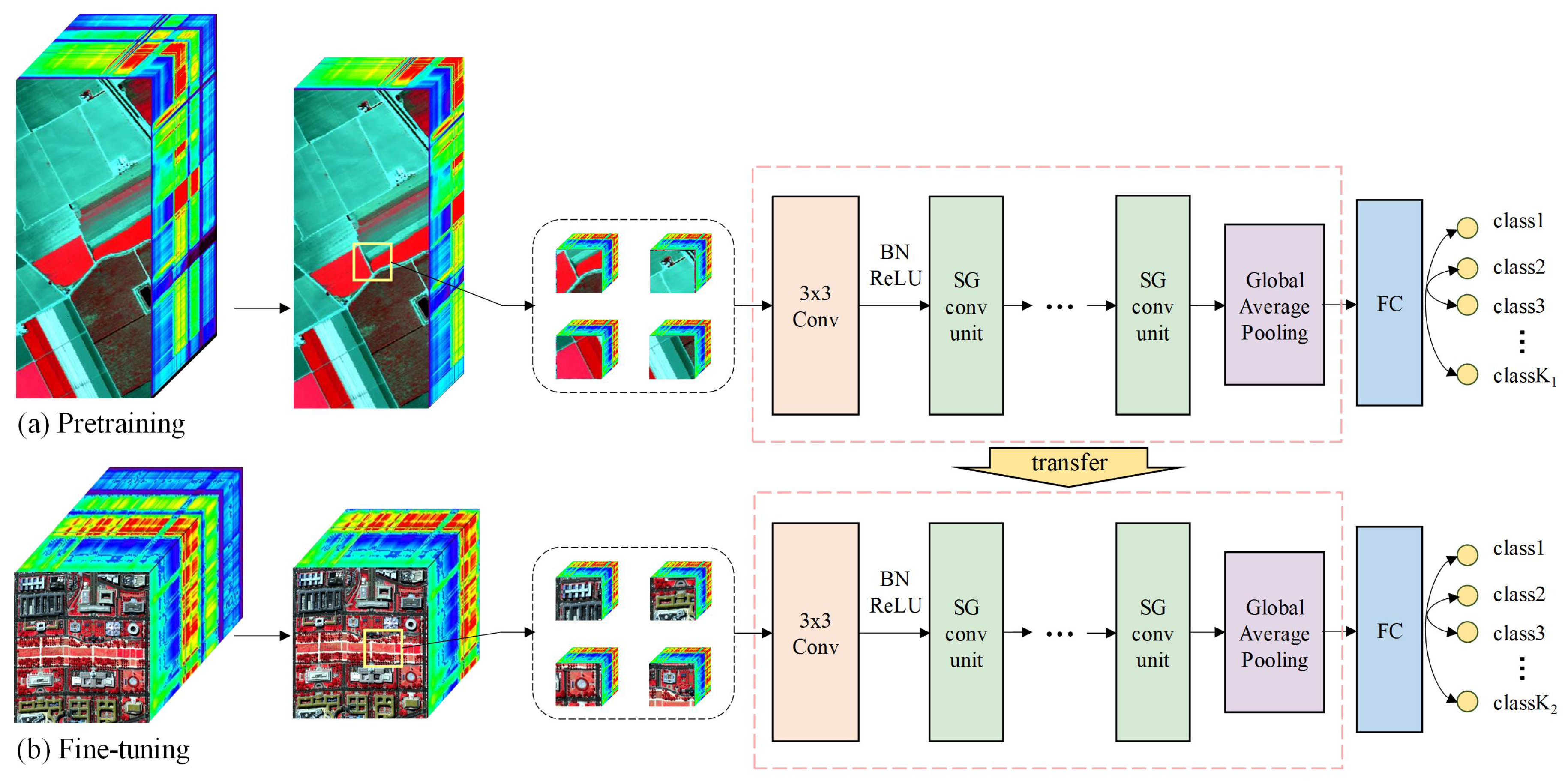
Three pairs of transfer learning experiments were designed using these six datasets: (1) pretrain on the Indian Pines, and fine-tune on the Botswana scene; (2) pretrain on the PaviaU scene, and fine-tune on the Houston 2013 scene; (3) pretrain on the Salinas scene, and fine-tune on the DC Mall scene. The experiments were designed as above for two reasons: (1) the source data and target data were collected by different sensors, but they were similar in terms of spatial resolution and the spectral range; (2) the source data have more labeled samples in each class than those of the target data. Despite that slight differences of band wavelengths may exist between the source and target data, SG-CNNs will automatically adapt its parameters to extract spectral features for the target data in the fine-tuning process.

3.2. Experimental Setup

To evaluate the performance of the proposed classification framework, classification results of three target datasets were compared with those predicted from two baseline models, i.e., ShuffleNet V2 (abbreviated as ShuffleNet2) [40] and ResNeXt [45]. ShuffleNet2 is well-known for its speed and accuracy tradeoff. ResNeXt consists of building blocks with group convolution and shortcut connections, which are also used in the SG-CNN. It is worth noting that we used ShuffleNet2 and ResNeXt with fewer building blocks rather than their original models, considering the limited samples of HSIs. Specifically, convolution layers in Stages 3 and 4 of ShuffleNet2 were removed, and output channels was set to 48 for Stage 2 layers; for the ResNeXt model, only one building block was retained. For further details on ShuffleNet2 and ResNeXt architectures, the reader is referred to [40,45]. In addition, simplified ShuffleNet2 and ResNeXt were both trained on the original target HSI data as well as fine-tuned on the 64-band target data using a corresponding pretrained network from the 64-band source data. Classification results obtained from the transfer learning of baseline models were referred to ShuffleNet2_T and ResNeXt_T, respectively. In addition, we performed transfer learning with SG-CNNs throughout the experiment.

Three SG-CNNs with three levels of complexity were tested for evaluation (see

Table 2. Overall SG-CNN architecture with different levels of complexity.

Basic Block	Channel Number	SG-CNN-7	SG-CNN-8	SG-CNN-12
Image	64	64	64	64
Conv	64	-	3 × 3, 64	-
SG conv unit 1	128	1 × 1, 64	1 × 1,64	1 × 1, 64
		3 × 3, 64, r = 1	3 × 3, 64, r = 1	3 × 3, 64, r = 1
		3 × 3, 64, r = 3	3 × 3, 64, r = 3	3 × 3, 64, r = 3
		3 × 3, 64, r = 5	3 × 3, 64, r = 5	3 × 3, 64, r = 5
		1 × 1, 128	1 × 1, 128	1 × 1, 128
SG conv unit 2	256			1 × 1,128
				3 × 3, 128, r = 1
				3 × 3, 128, r = 3
				3 × 3, 128, r = 5
				1 × 1, 256
FC	14/15/6
No. of trainable parameters		∼70,000	∼100,000	∼140,000

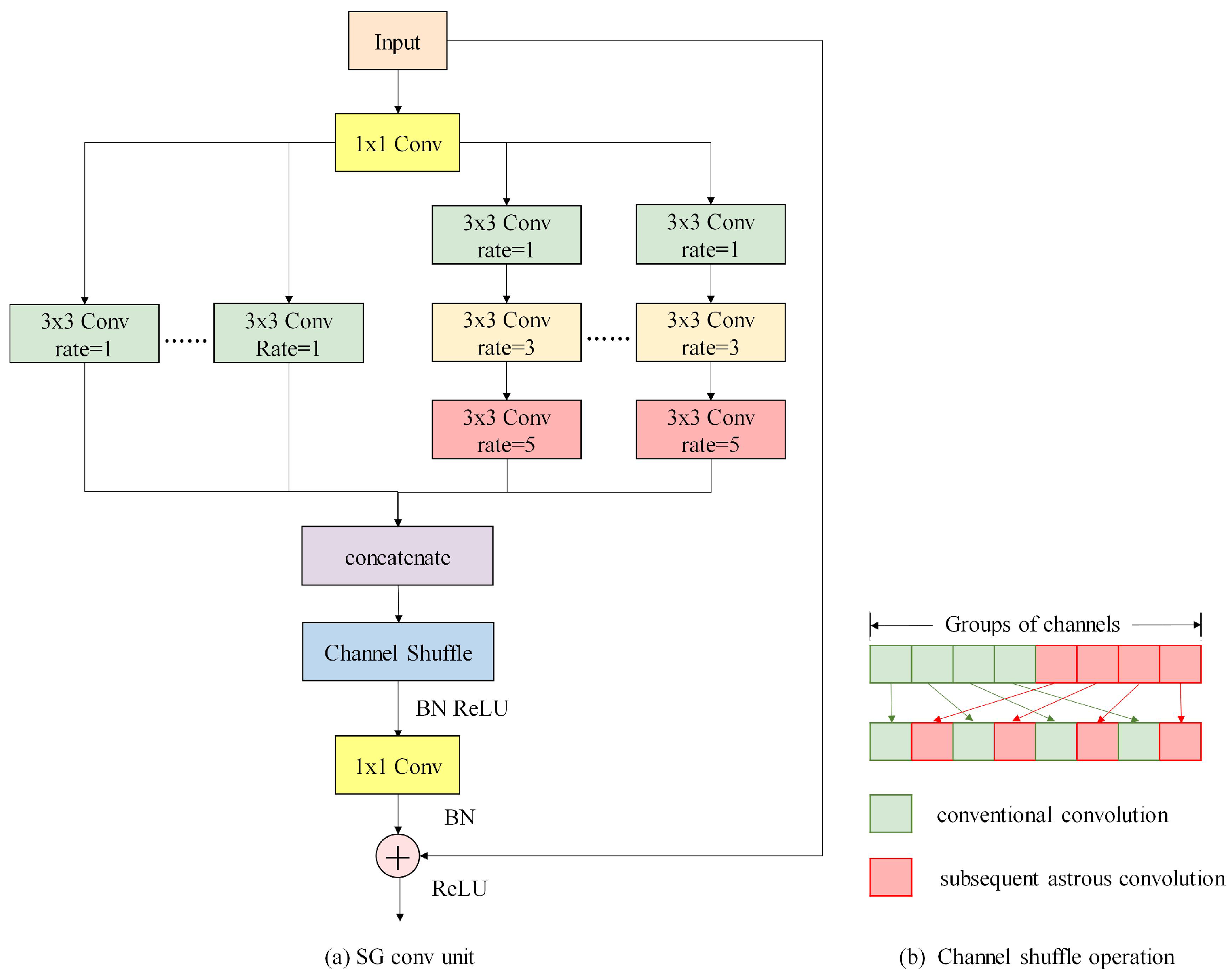
Groups that have conventional convolution in SG conv units are omitted in the table, as this operation is the same as the first layer of subsequent atrous convolution layers with a dilation rate of 1 (i.e., r = 1).

). SG-CNN-X represents the SG-CNN with X layers of convolution. It is worth noting that ResNeXt and SG-CNN-8 have the same number of layers, and the only difference between their structure is the introduction of atrous convolution for half the groups and shuffle operation in the SG-CNN-8 model. The number of groups was fixed to eight for both the SG-CNNs and ResNeXt, and the sample size was set to 19 × 19. In the SG conv unit, the dilation rates of three atrous convolutions were set to 1, 3, and 5 to get a receptive field of 19 (i.e., the full size of a sample).

Before network training, original data were normalized to guarantee input values within 0 to 1. Data augmentation techniques (including horizontal and vertical flip) were used to increase the training samples. All classification methods were implemented using python code with high-level APIs Tensorflow [48] and Keras. To further alleviate possible overfitting, the sum of multi-class cross entropy and L2 regularization term was taken as the loss function, and we set the weight decay to 5 × 10⁻⁴ in the L2 regularizer. The Adam optimizer [49] was adopted with an initial learning rate of 0.001, and the learning rate would be reduced to one-fifth of its value if the validation loss function did not decrease for 10 epochs. We used the Adam optimizer with a mini-batch size of 32 on a NVIDIA GEFORCE RTX 2080Ti GPU. The number of epochs was set to 150–250 for different datasets, and it is determined based on the number of training samples.

3.3. Experiments on Indian Pines and Botswana Scenes

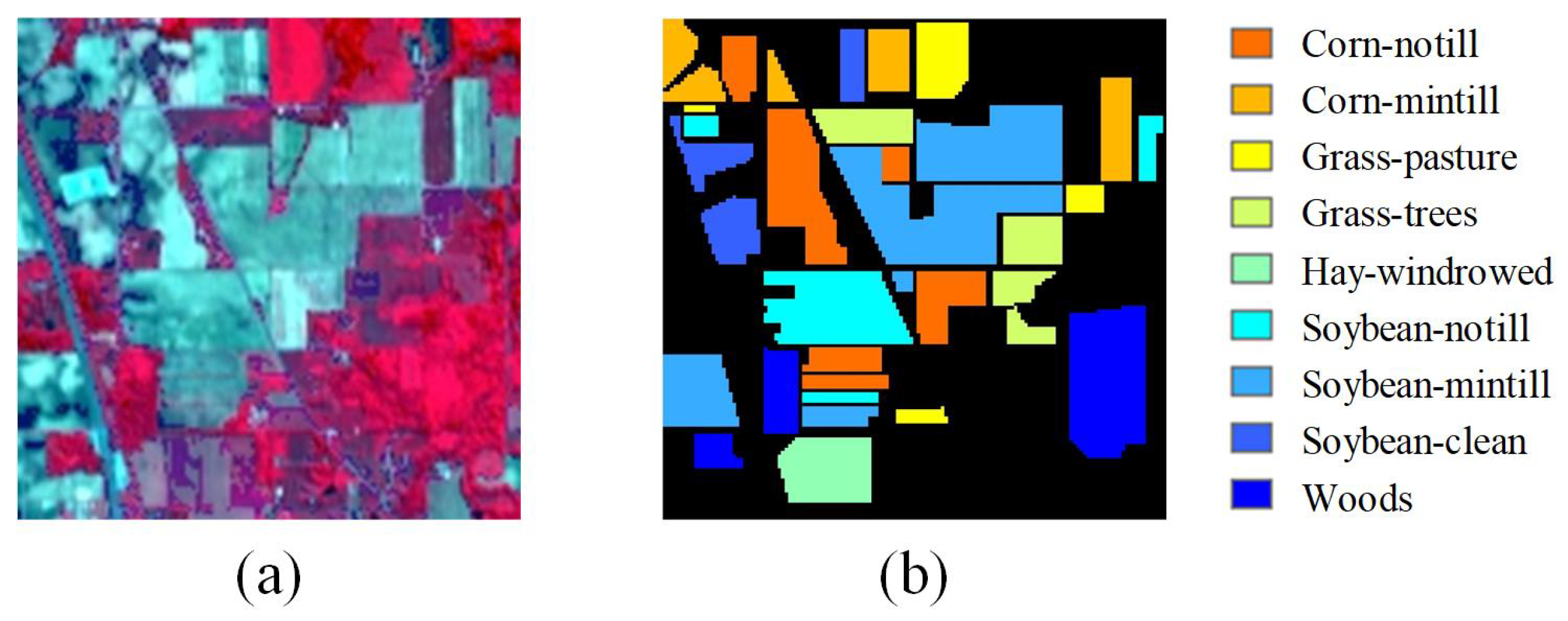
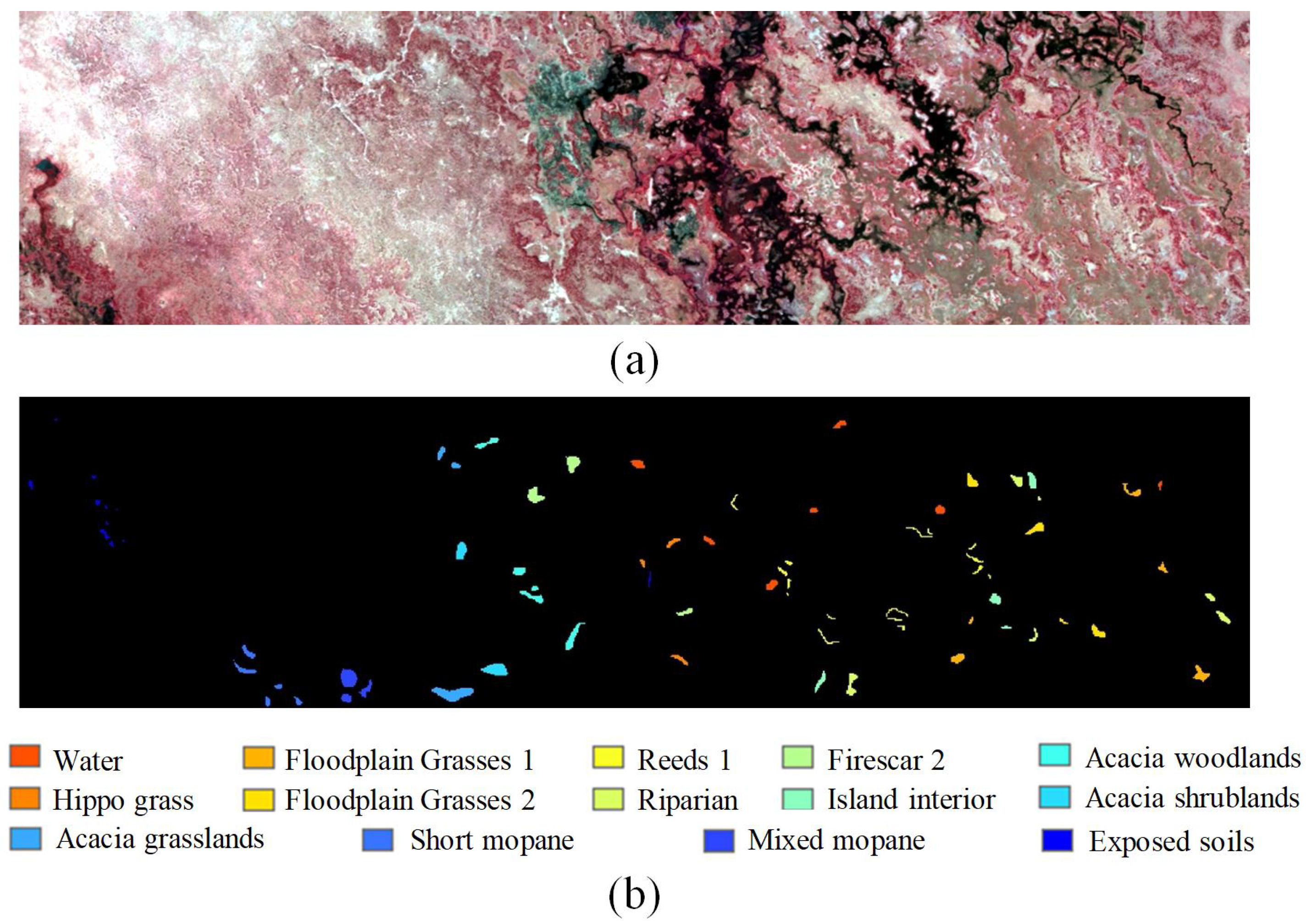
The false-color composites of the Indian Pines and Botswana scenes are displayed in Figure 4 and Figure 5, with their corresponding ground truth. In the pre-training and fine-tuning stage,

Table 3. The number of training and test samples used in Indiana Pines and Botswana datasets.

No.	Indian Pines			Botswana
	Class Name	Train	Test	Class Name	Train	Test
1	Corn-notill	200	1228	Water	30	240
2	Corn-mintill	200	630	Hippo grass	30	71
3	Grass-pasture	200	283	Floodplain Grasses 1	30	221
4	Grass-trees	200	530	Floodplain Grasses 2	30	185
5	Hay-windrowed	200	278	Reeds 1	30	239
6	Soybean-notill	200	772	Riparian	30	239
7	Soybean-mintill	200	2255	Firescar 2	30	229
8	Soybean-clean	200	393	Island interior	30	173
9	Woods	200	1065	Acacia woodlands	30	284
10				Acacia shrublands	30	218
11				Acacia grasslands	30	275
12				Short mopane	30	151
13				Mixed mopane	30	238
14				Exposed soils	30	65

gives the number of labeled pixels that were randomly selected for training, and the remaining labeled samples were used for the test.

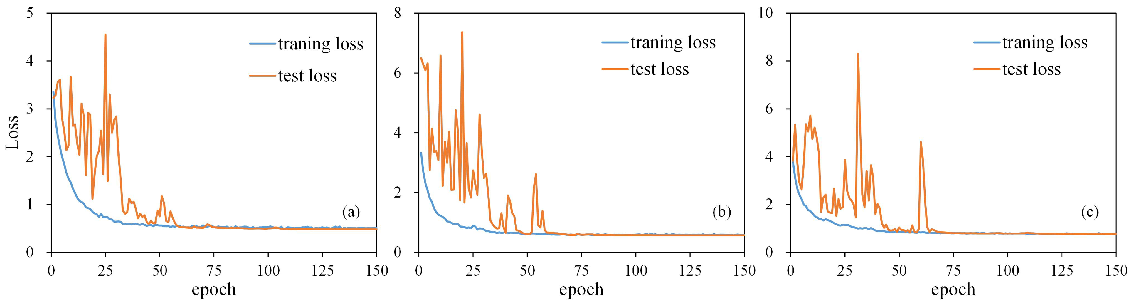
The loss function of SG-CNNs converged in the 150 epochs of training, indicating no overfitting during the fine-tuning process (see Figure 6). Classification results obtained by SG-CNNs were then compared with other methods in

Table 4. Classification accuracy (%) and computation time of the Botswana scene. A total of 420 labeled samples (30 per class) were used for fine-tuning. The No. column refers to the corresponding class in Table 3. The best results are in bold.

No.	ShuffleNet2	ShuffleNet2_T	ResNeXt	ResNeXt_T	SG-CNN-7	SG-CNN-8	SG-CNN-12
1	94.12	95.65	91.53	93.28	98.36	97.17	99.17
2	75.53	81.61	95.95	92.21	100.00	100.00	100.00
3	100.00	100.00	100.00	100.00	100.00	100.00	100.00
4	87.68	87.68	93.43	93.91	93.91	98.40	97.88
5	89.27	88.73	93.55	91.70	99.11	98.31	99.57
6	97.42	98.33	100.00	100.00	100.00	100.00	100.00
7	97.86	94.24	99.13	100.00	97.45	100.00	100.00
8	94.02	97.19	100.00	97.19	100.00	100.00	99.43
9	100.00	100.00	100.00	100.00	100.00	100.00	100.00
10	100.00	88.26	100.00	100.00	99.54	100.00	100.00
11	100.00	100.00	100.00	99.64	98.56	98.57	99.28
12	85.80	100.00	99.34	100.00	100.00	100.00	100.00
13	100.00	99.58	99.58	100.00	100.00	100.00	100.00
14	100.00	100.00	100.00	100.00	100.00	100.00	100.00
OA	95.33	95.44	98.06	97.91	98.97	99.36	99.65
AA	94.41	95.09	98.04	97.71	99.07	99.46	99.67
K	94.94	95.05	97.89	97.74	98.89	99.31	99.62
Time(s)	626.61	460.77	1591.27	375.60	524.25	389.06	1459.72

For the SG-CNNs, all classification results are obtained with fine-tuning on the target data based on a pretrained model using the source data.

for the Botswana scene. A range of criteria, including overall accuracy (OA), average accuracy (AA), and Kappa coefficient (K), were all reported as well as the classification accuracy of each class and training time. OA and AA are defined as below:

$$\begin{array}{c}\hfill OA=\frac{{\sum }_{i=1}^n{C}_i}{{\sum }_{i=1}^n{S}_i}\end{array}$$

(2)

$$\begin{array}{c}\hfill AA=\frac{1}{n}\sum _{i=1}^n\frac{C_i}{S_i}\end{array}$$

(3)

where $C_i$ is the number of correctly predicted samples out of $S_i$ samples in class i, and n is the number of classes.

Based on the results in Table 4, several preliminary conclusions can be drawn as follows.

(1) Compared with baseline models, SG-CNNs typically achieve better classification performance, providing higher accuracy and spending relatively less training time. Specifically, the overall accuracy of SG-CNNs was 98.97–99.65%, which was approximately ∼1% and ∼3.5% higher, on average, than ResNeXt and ShuffleNet2 models, respectively. In addition, SG-CNN-7 and SG-CNN-8 were shown to be quite efficient, as the execution time of their fine-tuning process was comparable to that of ShuffleNet2_T and ResNeXt_T. As an effect of its complicated structure with more trainable parameters, SG-CNN-12 required a longer period of time to fine-tune.

(2) As mentioned in Section 3.2, SG-CNN-8 can be seen as the baseline ResNeXt model that introduces atrous convolution and channel shuffle into its group convolution. Comparing the classification results of these two models, we can appreciate that the inclusion of atrous convolution and channel shuffle improved the classification.

(3) For the baseline models, both ShuffleNet2_T and ResNeXt_T, which were fine-tuned on the 64-band target data, obtained similar accuracy with much lower execution time, compared with their counterparts that were directly trained from original HSIs. This indicates that the simple band selection strategy applied in transfer learning can generally help to enhance the training efficiency.

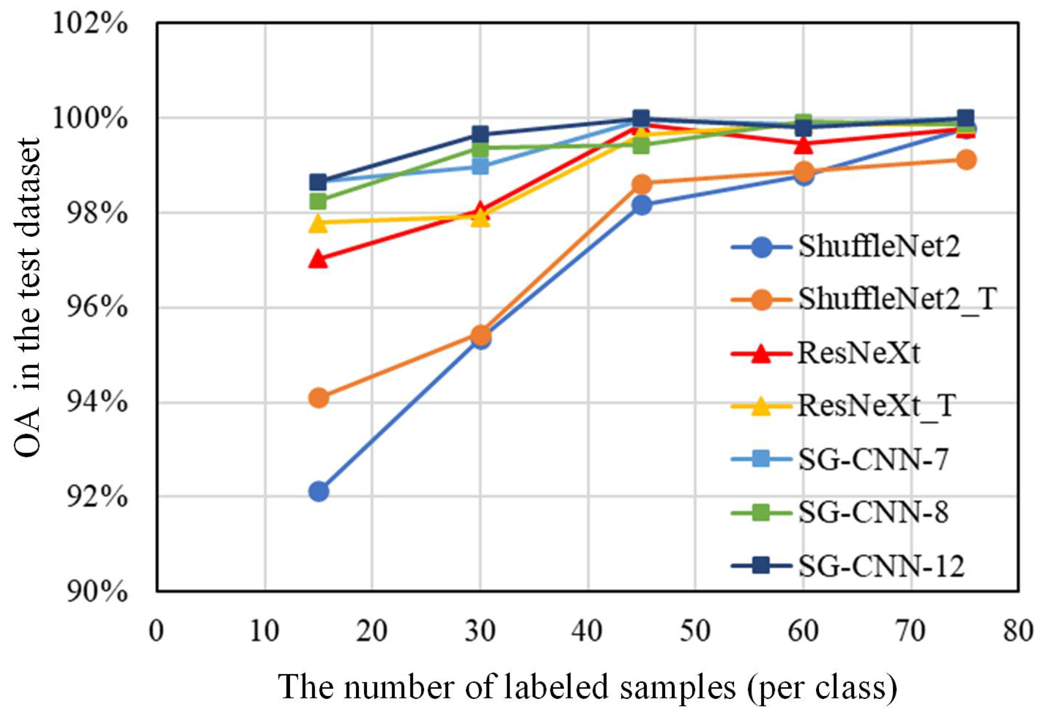
Our second test with the Botswana scene evaluated the classification performance of transfer learning with SG-CNNs using varying sizes of samples. Specifically, 15, 30, 45, 60, and 75 samples per class from the Botswana scene were used, respectively, to fine-tune the pretrained SG-CNNs, and their classification performances were evaluated from OAs of the corresponding remaining samples (i.e., the test samples). Meanwhile, the same samples used for fine-tuning SG-CNNs were utilized to train ShuffleNet2 and ResNext and fine-tune ShuffleNet2_T and ResNext_T. These models were also assessed with OA of test samples. Figure 7 displays OAs in the test dataset from different classification methods with different numbers of training samples. Several conclusions can be drawn:

(1) Compared with ShuffleNet2, ShuffleNet2_T, and ResNeXt, SG-CNNs showed a remarkable improvement for classification by providing a higher classification accuracy, especially when labeled samples were relatively small (i.e., 15–60 samples per class).

(2) Compared with ResNeXt_T, SG-CNNs generally yielded better classification results when the training samples were limited (i.e., 15–45 per class). As the number of samples increased to 60–75 for each class, ResNeXt_T provided comparable accuracy.

(3) Although SG-CNN-12 generally achieved the best performance, its classification accuracy was merely 0.1–0.7% higher than that of SG-CNN-7 and SG-CNN-8. However, the latter two showed smaller values of execution time for the fine-tuning than the former. In other words, SG-CNN-7 and SG-CNN-8 had better tradeoffs between classification accuracy and efficiency.

3.4. Experiments on PaviaU and Houston 2013 Scenes

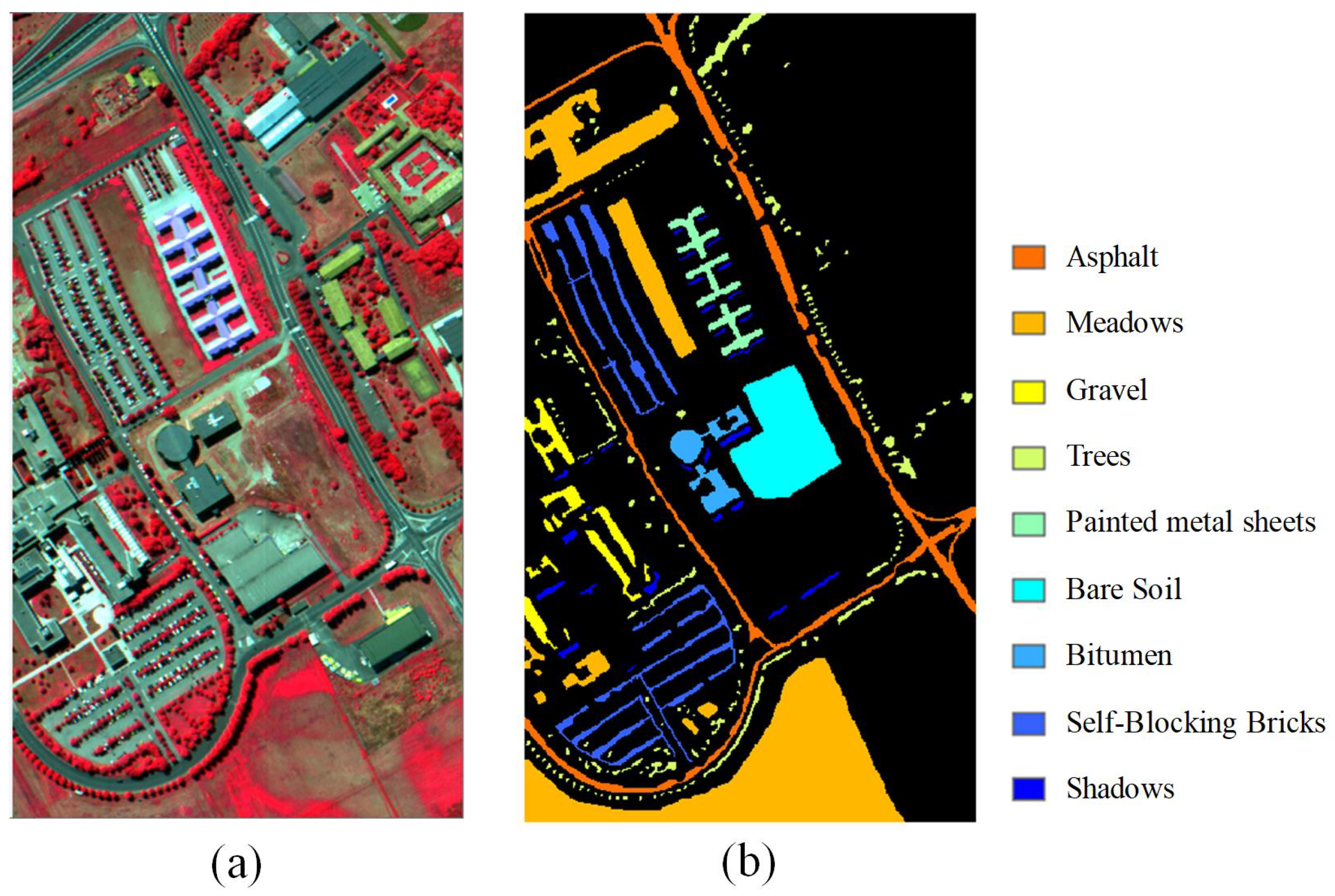
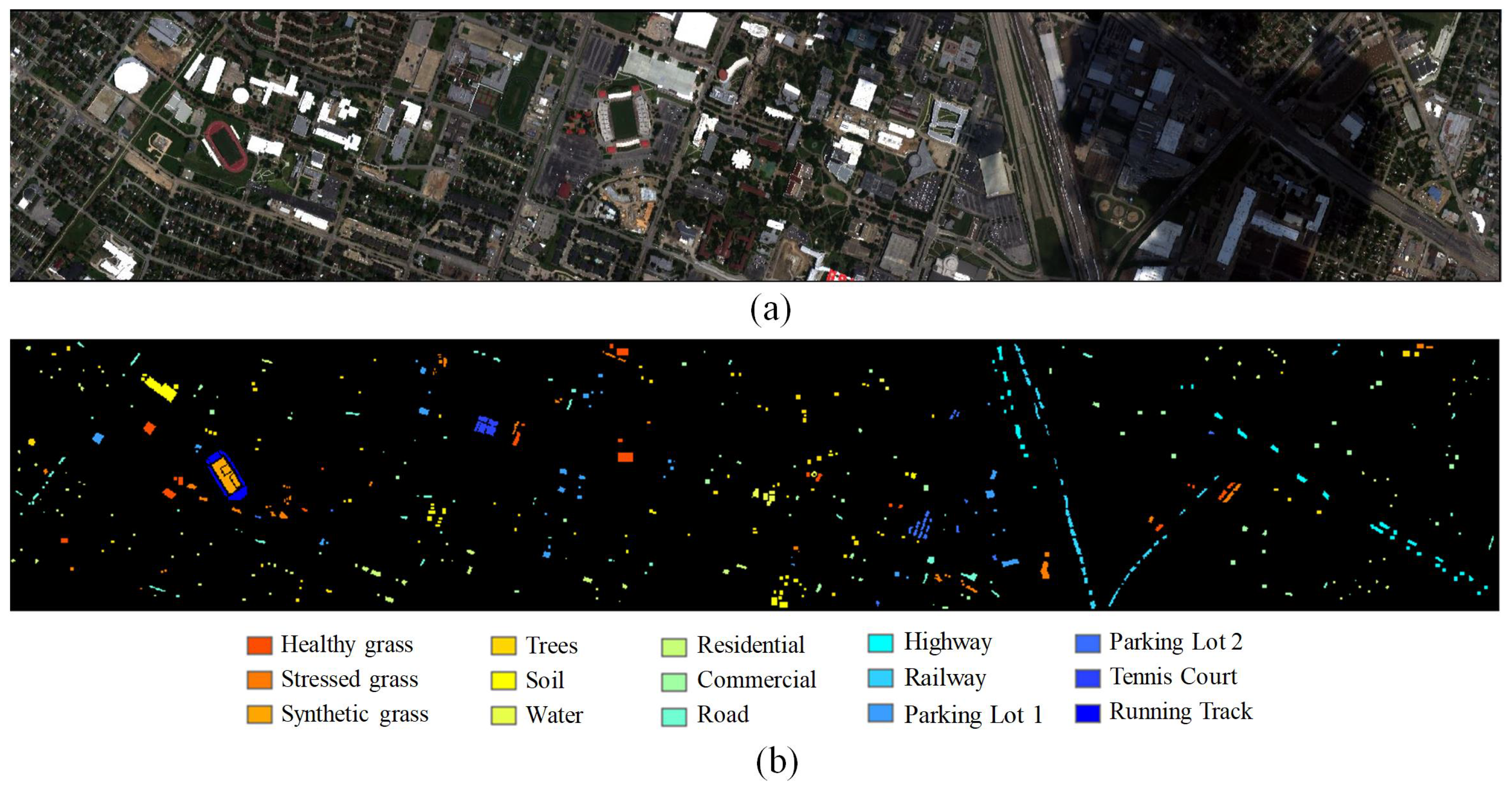
PaviaU and Houston 2013 datasets are displayed with their labeled sample distributions in Figure 8 and Figure 9. Figure 8 shows that the PaviaU scene contained five manmade types, two types of vegetation, and one type for soil and shadow. As shown in Figure 9, the Houston 2013 scene had nine manmade types, four types of vegetation, and one type for soil and water. Surface types distributions were similar in these two scenes. ShuffleNet2, ResNeXt, and SG-CNNs were fine-tuned on the Houston 2013 scene, with pretrained models acquired from training with the PaviaU dataset.

Table 5. The number of training and test samples for PaviaU and Houston 2013 datasets.

No.	PaviaU			Houston 2013
	Class Name	Train	Test	Class Name	Train	Test
1	Asphalt	600	6031	Healthy grass	100	1151
2	Meadows	600	18,049	Stressed grass	100	1154
3	Gravel	600	1499	Synthetic grass	100	597
4	Trees	600	2464	Trees	100	1144
5	Painted metal sheets	600	745	Soil	100	1142
6	Bare soil	600	4429	Water	100	225
7	Bitumen	600	730	Residential	100	1168
8	Self-Blocking Bricks	600	3082	Commercial	100	1144
9	Shadows	600	347	Road	100	1152
10				Highway	100	1127
11				Railway	100	1135
12				Parking Lot 1	100	1133
13				Parking Lot 2	100	369
14				Tennis Court	100	328
15				Running Track	100	560

displays the number of samples used in the experiment, respectively. Six hundred labeled samples per class in the PaviaU scene were utilized to pretrain the models, whereas 100 randomly selected samples per class in the Houston scene were used for fine-tuning.

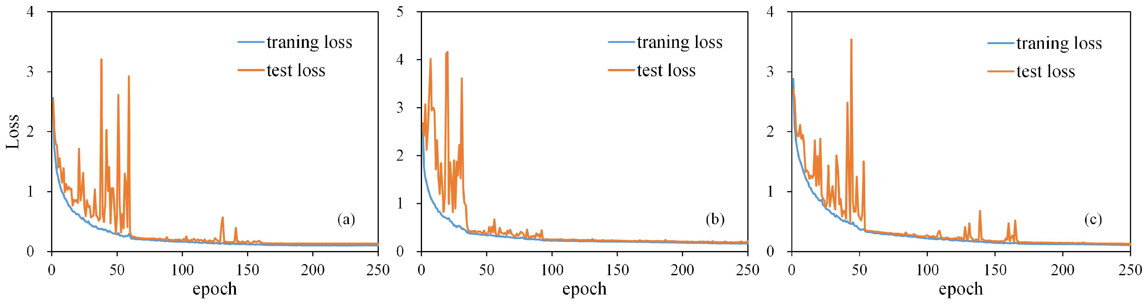
Convergence curves of the loss function are shown in Figure 10 for the fine-tuning of SG-CNNs applied to the Houston 2013 scene. Classification results acquired from SG-CNNs and baseline models are detailed in

Table 6. Classification accuracy (%) and computation time of the Houston 2013 scene. A total of 1500 labeled samples (100 per class) were used for fine-tuning. The No. column refers to the corresponding class in Table 5. The best results are in bold.

No.	ShuffleNet2	ShuffleNet2_T	ResNeXt	ResNeXt_T	SG-CNN-7	SG-CNN-8	SG-CNN-12
1	90.09	91.54	84.71	92.65	99.83	97.62	99.74
2	92.33	99.28	97.77	96.72	99.65	99.65	99.40
3	90.73	99.66	99.66	99.83	100.00	99.83	100.00
4	97.28	99.22	96.87	99.08	99.91	99.82	100.00
5	100.00	98.87	99.22	99.22	100.00	99.65	99.22
6	89.36	97.38	83.08	93.75	95.34	95.34	97.40
7	87.18	94.65	92.60	94.84	98.29	100.00	100.00
8	99.30	97.99	98.84	99.46	100.00	89.22	99.82
9	86.49	93.46	88.50	96.99	97.62	96.69	97.86
10	92.15	96.24	94.15	94.47	99.20	98.41	99.64
11	95.37	94.00	97.07	97.88	100.00	100.00	100.00
12	92.50	96.65	100.00	97.00	95.94	89.26	99.47
13	97.43	93.26	95.65	100.00	100.00	100.00	100.00
14	100.00	84.75	100.00	100.00	100.00	100.00	100.00
15	95.87	97.38	96.54	96.88	97.22	97.90	97.73
OA	93.27	95.92	94.95	97.02	98.98	97.18	99.45
AA	93.74	95.62	94.98	97.25	98.87	97.56	99.40
K	92.71	95.58	94.53	96.77	98.90	96.94	99.35
Time(s)	2068.42	1614.16	5120.20	2309.30	2088.32	1035.15	2957.94

. As shown in Table 6, SG-CNNs with different levels of complexity achieved higher classification accuracies than those of ShuffleNet2, ShuffleNet2_T, ResNeXt, and ResNeXt_T. Specifically, SG-CNN-12 provided the best classification results with the highest OA (99.45%), AA (99.40%), and Kappa coefficient (99.35%), and it also achieved the highest classification accuracy for eight classes in the test samples. Comparing the results from SG-CNN-8 and ResNeXt_T, the former obtained a slightly higher OA than the latter but spent less than half the training time, indicating the SG conv unit’s effectiveness for classification improvement. In addition, fine-tuned ResNeXt_T and ShuffleNet2_T yielded better results than the original ResNeXt and ShuffleNet2. Hence, this confirms the previous conclusion that our band selection strategy applied in transfer learning boosts the classification performance.

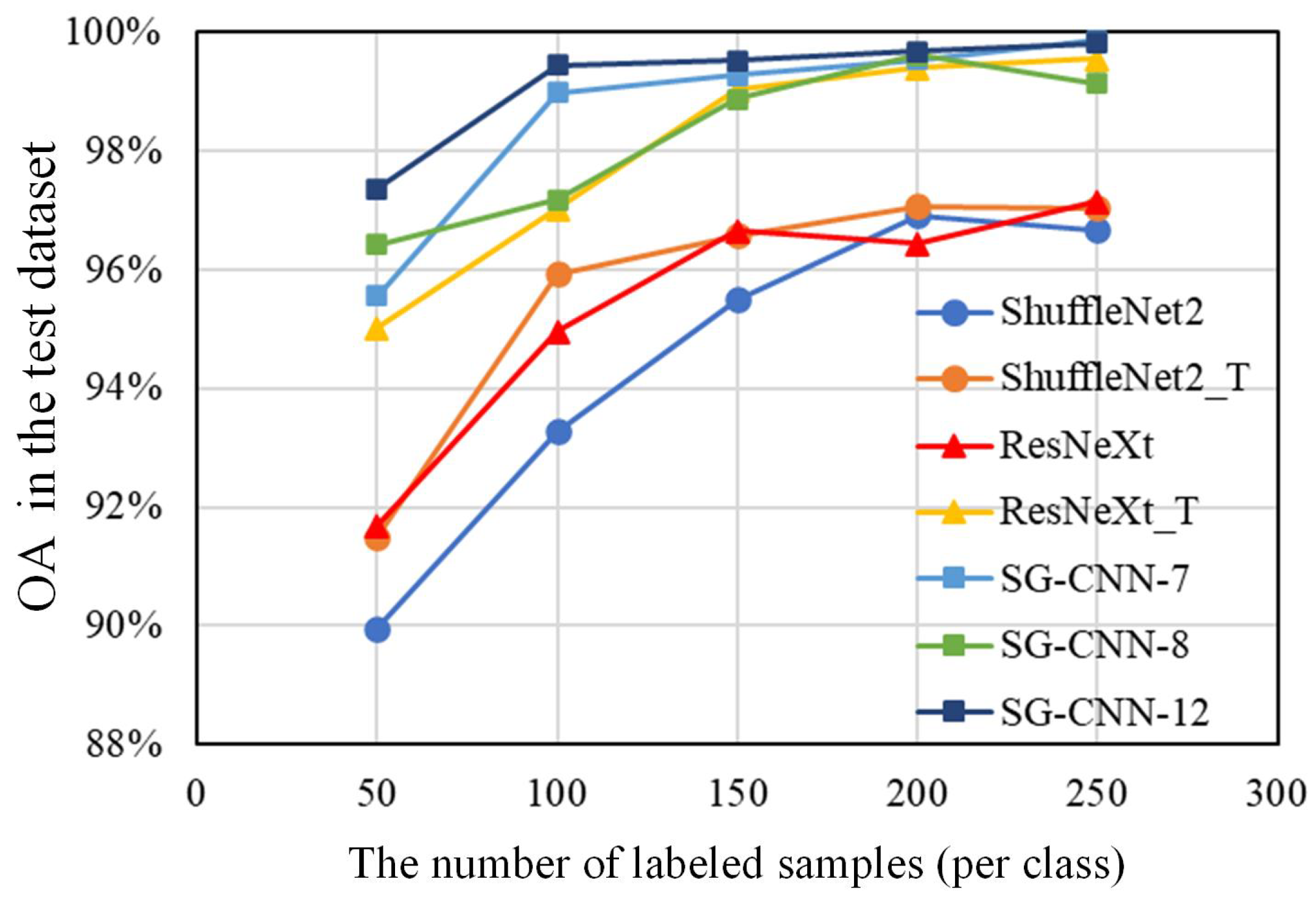
Classification experiments with varying numbers of training samples were also conducted. Specifically, 50–250 samples per class in the Houston scene were used for fine-tuning the SG-CNNs, as well as for training or fine-tuning the baseline networks. OAs of the remaining test samples are shown in Figure 11 for all the methods. Some conclusions can be reached from making comparisons between these results:

(1) As training samples varied from 50 to 250 per class, SG-CNNs outperformed ShuffleNet2, ShuffleNet2_T, and ResNeXt for the Houston 2013 scene classification. The accuracies of the fine-tuned SG-CNNs are ∼1.3–7.4% higher than that of the other three baseline networks, indicating that SG-CNNs greatly improved the classification performance with both limited and sufficient samples.

(2) Comparing with ResNeXt_T, SG-CNNs obtained better results when few samples were provided (i.e., 50–100 per class). As the number of samples increased to 150–250 per class, the ResNeXt_T and SG-CNNs achieved comparable accuracy. This suggests that SG-CNNs have better performance with limited samples.

(3) In general, SG-CNN-12 provided the highest classification accuracy among the three SG-CNNs. However, as the number of training samples increased, the performance of SG-CNN-12 showed no obvious improvement compared to SG-CNN-7 and SG-CNN-8, which are more efficient and require less computing time.

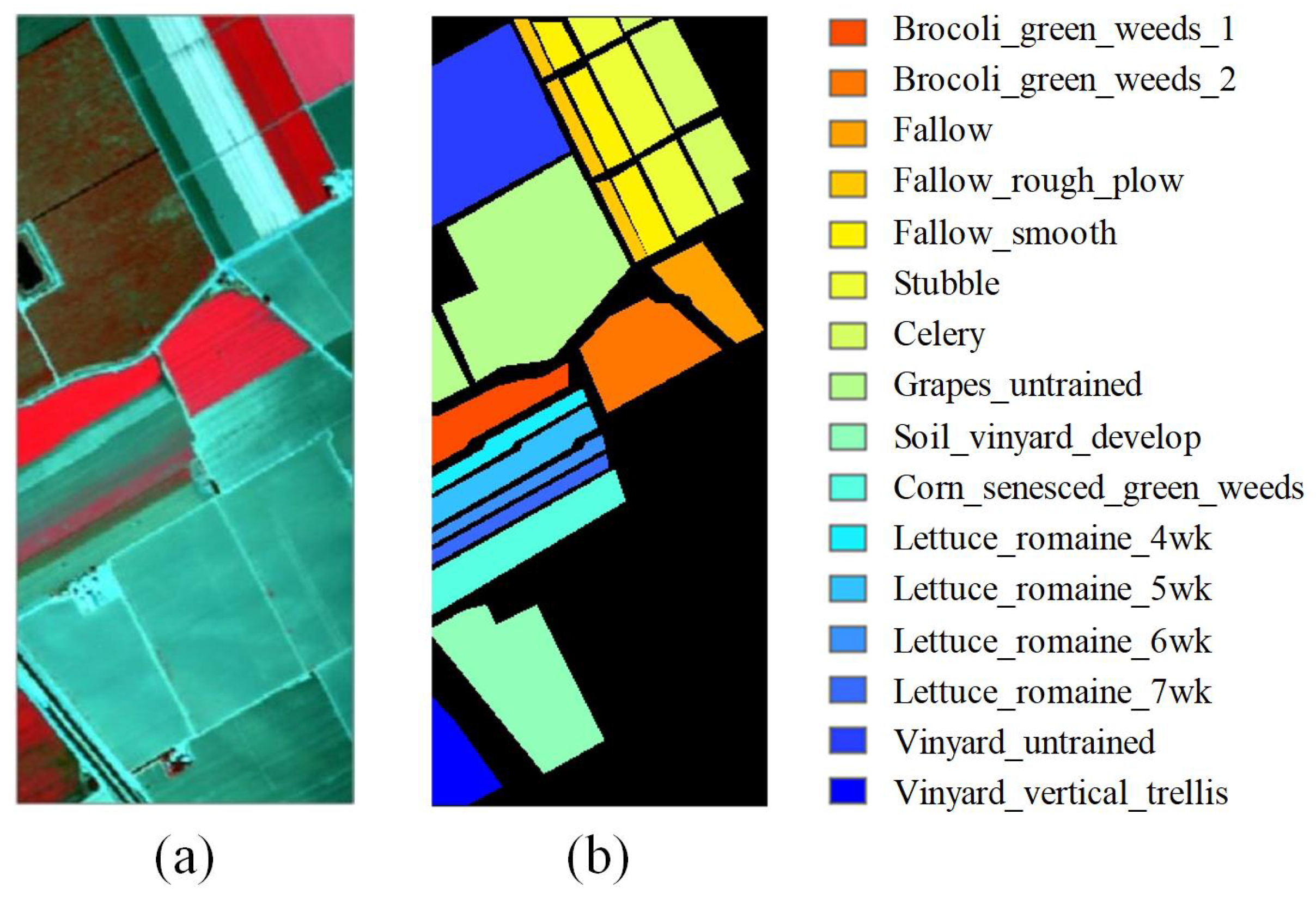
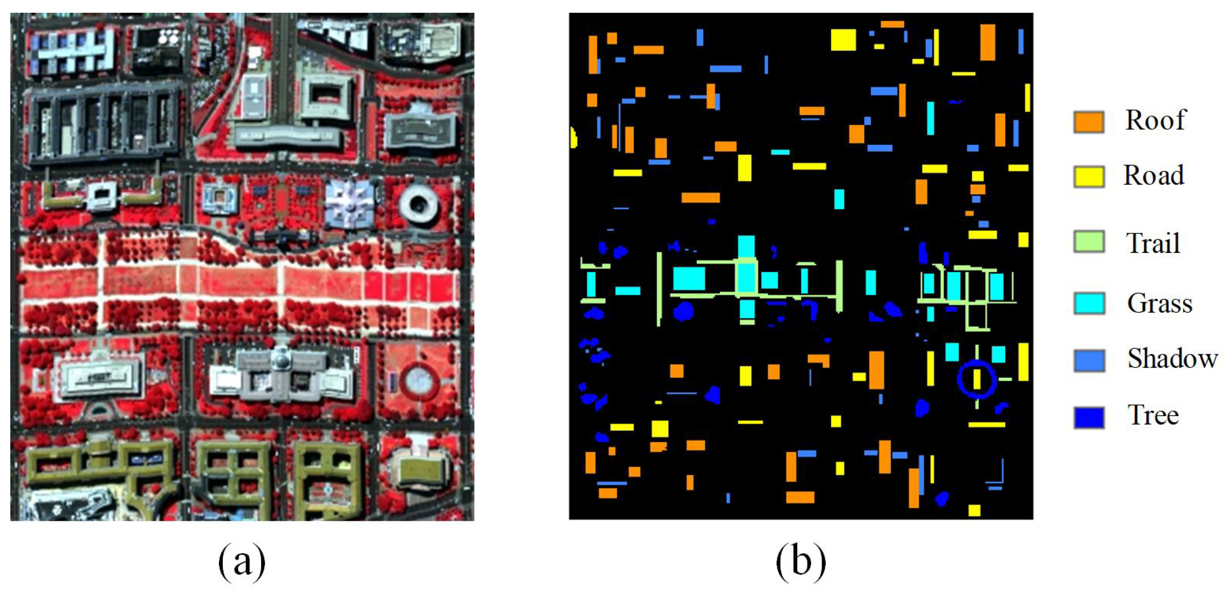
3.5. Experiments on Salinas and DC Mall Scenes

Salinas and DC Mall images and their labeled samples are shown in Figure 12 and Figure 13, respectively. It is important to note that surface types were quite different between these two scenes. The Salinas scene mainly consisted of natural materials (i.e., vegetation and three types of fallow), whereas the DC Mall scene included grass, trees, shadows, and three manmade materials.

Table 7. The number of training and test samples for Salinas and DC Mall datasets.

No.	Salinas			DC Mall
	Class Name	Train	Test	Class Name	Train	Test
1	Brocoli_green_weeds_1	500	1309	Roof	100	2816
2	Brocoli_green_weeds_2	500	3226	Grass	100	1719
3	Fallow	500	1476	Road	100	1164
4	Fallow_rough_plow	500	1194	Trail	100	1690
5	Fallow_smooth	500	2178	Tree	100	1020
6	Stubble	500	3459	Shadow	100	1181
7	Celery	500	3079
8	Grapes_untrained	500	10,771
9	Soil_vinyard_develop	500	5703
10	Corn_senesced_green_weeds	200	2778
11	Lettuce_romaine_4wk	500	568
12	Lettuce_romaine_5wk	500	1327
13	Lettuce_romaine_6wk	500	416
14	Lettuce_romaine_7wk	500	570
15	Vinyard_untrained	500	6768
16	Vinyard_vertical_trellis	500	1307

provides the number of samples used as training and test datasets. Five hundred samples of each class in the Salinas scene were randomly selected for base network training, whereas 100 samples of each class in the DC Mall scene were used for fine-tuning.

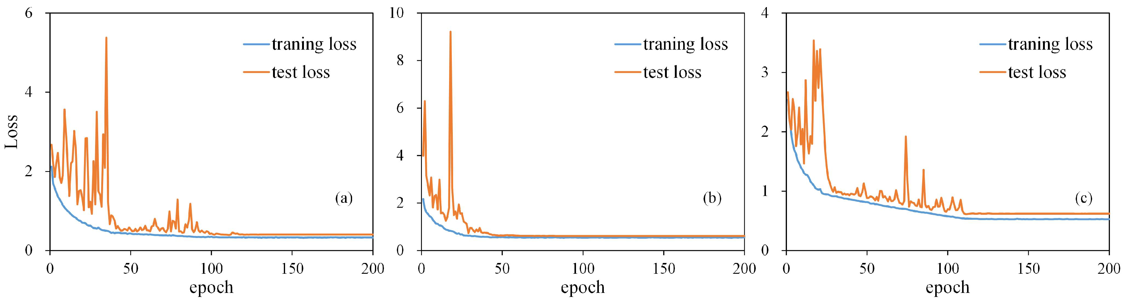
The loss function of SG-CNNs converged during the fine-tuning for the DC Mall scene (see Figure 14). The classification results of both baseline models and SG-CNNs are listed in

Table 8. Classification accuracy (%) and computation time of the DC Mall scene. A total of 600 labeled samples (100 per class) were used for fine-tuning. The No. column refers to the corresponding class in Table 7. The best results are in bold.

No.	ShuffleNet2	ShuffleNet2_T	ResNeXt	ResNeXt_T	SG-CNN-7	SG-CNN-8	SG-CNN-12
1	90.90	91.50	89.65	96.65	98.46	99.77	99.47
2	92.03	91.02	90.96	92.14	93.47	92.77	94.85
3	77.57	76.34	66.87	78.18	92.49	95.53	93.37
4	94.21	92.16	89.44	92.20	99.19	99.51	99.45
5	50.53	52.23	51.79	65.93	80.67	90.19	92.63
6	92.17	91.69	89.85	95.34	97.42	99.24	99.58
OA	83.89	83.22	80.67	88.18	94.60	96.68	97.06
AA	82.90	82.49	79.76	86.74	93.62	96.17	96.56
K	80.31	79.53	76.39	85.53	93.36	95.92	96.38
Time(s)	2535.16	1660.96	4310.51	2670.86	1133.61	885.03	2324.81

with their corresponding training time. As shown in Table 8, similar conclusions can be reached from the DC Mall experiment. First, SG-CNNs outperformed the baseline models in terms of classification results. Moreover, SG-CNN-8 had an OA nearly 10% higher than that of ResNeXt_T, indicating the improvement brought by the proposed SG conv unit. Furthermore, although the target data and source data had different surface types, transfer learning on the SG-CNNs led to major improvement in the classification accuracy.

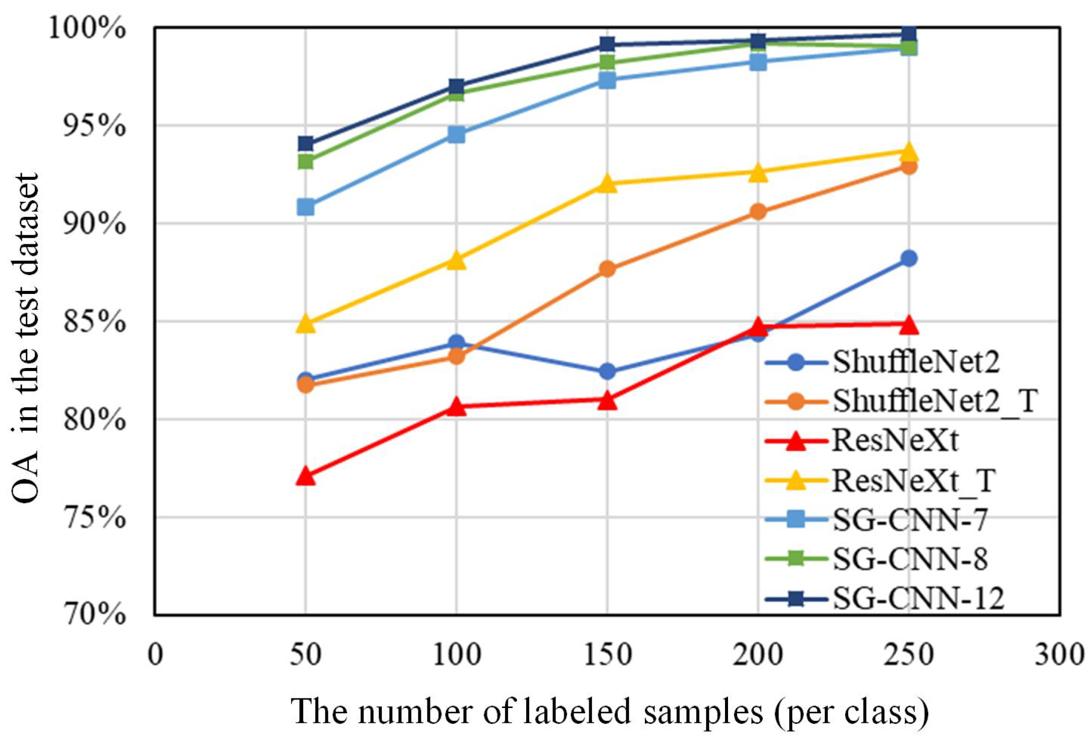
Analogously, our second test on the DC Mall scene evaluated the classification performance of the proposed method with varying sizes of labeled samples. We used 50–250 samples per class at an interval of 50 to train ShuffleNet2 and ResNeXt and to fine-tune SG-CNNs, ShuffleNet2_T, and ResNeXt_T. Figure 15 shows the OAs for the test samples from all methods. In the DC Mall experiment, SG-CNNs outperformed all baseline models, including the ResNeXt_T, when a large number of training samples (e.g., 250 samples per class) was provided. Specifically, the OA of SG-CNNs was higher than that of other methods by 5.3–18.2%, which confirmed the superiority of our proposed method. For the DC Mall dataset, SG-CNN-12 achieved better results when samples were relatively limited (i.e., 50–150 samples per class). With 200–250 training samples in each category, SG-CNN-7 and SG-CNN-8 required less time to obtain a comparable accuracy to that of SG-CNN-12.

4. Conclusions

Typically, only limited labeled samples are available for HSI classification. To improve the HSI classification for such conditions, we proposed a new CNN-based classification method that performed transfer learning between different HSI datasets on a proposed lightweight CNN. This scheme, named SG-CNN, consisted of SG conv units, which combined group convolution, atrous convolution, and channel shuffle operation. In the SG conv unit, group convolution was utilized to reduce the number of parameters, while channel shuffle was employed to connect information in different groups. Also, atrous convolution was introduced in addition to conventional convolution in the groups so that the receptive field was enlarged. To further improve the classification performance with limited samples, transfer learning was applied on SG-CNNs, with a simple dimensionality reduction implemented to keep the dimensions of input data consistent for both the source and target data.

To evaluate the classification performance of the proposed method, transfer learning experiments were performed on SG-CNNs between three pairs of public HSI scenes. Specifically, three SG-CNNs with different levels of complexity were tested. Compared with ShuffleNet-V2, ResNeXt, and their fine-tuned models, the proposed method considerably improved classification results when the training samples were limited, and it also enhanced model efficiency by reducing the computing cost for the training process. It suggests that the combination of atrous convolution with group convolution is effective for training with limited samples, and the band selection method can be helpful for transfer learning.

References

1. Zhang, B.; Wu, D.; Zhang, L.; Jiao, Q.; Li, Q. Application of hyperspectral remote sensing for environment monitoring in mining areas. Environ. Earth Sci. 2012, 65, 649–658. [Google Scholar] [CrossRef]
2. Kudela, R.M.; Palacios, S.L.; Austerberry, D.C.; Accorsi, E.K.; Guild, L.S.; Torres-Perez, J. Application of hyperspectral remote sensing to cyanobacterial blooms in inland waters. Remote Sens. Environ. 2015, 167, 196–205. [Google Scholar] [CrossRef] [Green Version]
3. Sankey, T.; Donager, J.; McVay, J.; Sankey, J.B. UAV lidar and hyperspectral fusion for forest monitoring in the southwestern USA. Remote Sens. Environ. 2017, 195, 30–43. [Google Scholar] [CrossRef]
4. Olmanson, L.G.; Brezonik, P.L.; Bauer, M.E. Airborne hyperspectral remote sensing to assess spatial distribution of water quality characteristics in large rivers: The Mississippi River and its tributaries in Minnesota. Remote Sens. Environ. 2013, 130, 254–265. [Google Scholar] [CrossRef]
5. Yokoya, N.; Chan, J.C.W.; Segl, K. Potential of resolution-enhanced hyperspectral data for mineral mapping using simulated EnMAP and Sentinel-2 images. Remote Sens. 2016, 8, 172. [Google Scholar] [CrossRef] [Green Version]
6. Makki, I.; Younes, R.; Francis, C.; Bianchi, T.; Zucchetti, M. A survey of landmine detection using hyperspectral imaging. ISPRS J. Photogramm. Remote Sens. 2017, 124, 40–53. [Google Scholar] [CrossRef]
7. Datt, B.; McVicar, T.R.; Van Niel, T.G.; Jupp, D.L.; Pearlman, J.S. Preprocessing EO-1 Hyperion hyperspectral data to support the application of agricultural indexes. IEEE Trans. Geosci. Remote Sens. 2003, 41, 1246–1259. [Google Scholar] [CrossRef] [Green Version]
8. Gevaert, C.M.; Suomalainen, J.; Tang, J.; Kooistra, L. Generation of spectral–temporal response surfaces by combining multispectral satellite and hyperspectral UAV imagery for precision agriculture applications. IEEE J. Sel. Top. Appl. Earth Obs. Remote Sens. 2015, 8, 3140–3146. [Google Scholar] [CrossRef]
9. Adão, T.; Hruška, J.; Pádua, L.; Bessa, J.; Peres, E.; Morais, R.; Sousa, J.J. Hyperspectral imaging: A review on UAV-based sensors, data processing and applications for agriculture and forestry. Remote Sens. 2017, 9, 1110. [Google Scholar] [CrossRef] [Green Version]
10. Gewali, U.B.; Monteiro, S.T.; Saber, E. Machine learning based hyperspectral image analysis: A survey. arXiv 2018, arXiv:1802.08701. [Google Scholar]
11. Melgani, F.; Bruzzone, L. Classification of hyperspectral remote sensing images with support vector machines. IEEE Trans. Geosci. Remote Sens. 2004, 42, 1778–1790. [Google Scholar] [CrossRef] [Green Version]
12. Kuching, S. The performance of maximum likelihood, spectral angle mapper, neural network and decision tree classifiers in hyperspectral image analysis. J. Comput. Sci. 2007, 3, 419–423. [Google Scholar]
13. Fauvel, M.; Tarabalka, Y.; Benediktsson, J.A.; Chanussot, J.; Tilton, J.C. Advances in spectral-spatial classification of hyperspectral images. Proc. IEEE 2012, 101, 652–675. [Google Scholar] [CrossRef] [Green Version]
14. Yu, H.; Gao, L.; Li, J.; Li, S.S.; Zhang, B.; Benediktsson, J.A. Spectral-spatial hyperspectral image classification using subspace-based support vector machines and adaptive markov random fields. Remote Sens. 2016, 8, 355. [Google Scholar] [CrossRef] [Green Version]
15. Yu, H.; Gao, L.; Liao, W.; Zhang, B.; Zhuang, L.; Song, M.; Chanussot, J. Global spatial and local spectral similarity-based manifold learning group sparse representation for hyperspectral imagery classification. IEEE Trans. Geosci. Remote Sens. 2020, 58, 3043–3056. [Google Scholar] [CrossRef]
16. Li, S.; Song, W.; Fang, L.; Chen, Y.; Ghamisi, P.; Benediktsson, J.A. Deep learning for hyperspectral image classification: An overview. IEEE Trans. Geosci. Remote Sens. 2019, 57, 6690–6709. [Google Scholar] [CrossRef] [Green Version]
17. Zhang, L.; Zhang, L.; Tao, D.; Huang, X. Tensor discriminative locality alignment for hyperspectral image spectral–spatial feature extraction. IEEE Trans. Geosci. Remote Sens. 2012, 51, 242–256. [Google Scholar] [CrossRef]
18. Chen, Y.; Lin, Z.; Zhao, X.; Wang, G.; Gu, Y. Deep learning-based classification of hyperspectral data. IEEE J. Sel. Top. Appl. Earth Obs. Remote Sens. 2014, 7, 2094–2107. [Google Scholar] [CrossRef]
19. Liu, Y.; Cao, G.; Sun, Q.; Siegel, M. Hyperspectral classification via deep networks and superpixel segmentation. Int. J. Remote Sens. 2015, 36, 3459–3482. [Google Scholar] [CrossRef]
20. Ma, X.; Wang, H.; Geng, J. Spectral–spatial classification of hyperspectral image based on deep auto-encoder. IEEE J. Sel. Top. Appl. Earth Obs. Remote Sens. 2016, 9, 4073–4085. [Google Scholar] [CrossRef]
21. Hu, W.; Huang, Y.; Wei, L.; Zhang, F.; Li, H. Deep convolutional neural networks for hyperspectral image classification. J. Sens. 2015, 2015, 1–12. [Google Scholar] [CrossRef] [Green Version]
22. Chen, Y.; Jiang, H.; Li, C.; Jia, X.; Ghamisi, P. Deep feature extraction and classification of hyperspectral images based on convolutional neural networks. IEEE Trans. Geosci. Remote Sens. 2016, 54, 6232–6251. [Google Scholar] [CrossRef] [Green Version]
23. Paoletti, M.E.; Haut, J.M.; Plaza, J.; Plaza, A. A new deep convolutional neural network for fast hyperspectral image classification. ISPRS J. Photogramm. Remote Sens. 2018, 145, 120–147. [Google Scholar] [CrossRef]
24. Mou, L.; Ghamisi, P.; Zhu, X.X. Deep recurrent neural networks for hyperspectral image classification. IEEE Trans. Geosci. Remote Sens. 2017, 55, 3639–3655. [Google Scholar] [CrossRef] [Green Version]
25. Liu, Q.; Zhou, F.; Hang, R.; Yuan, X. Bidirectional-convolutional LSTM based spectral-spatial feature learning for hyperspectral image classification. Remote Sens. 2017, 9, 1330. [Google Scholar] [CrossRef] [Green Version]
26. Krizhevsky, A.; Sutskever, I.; Hinton, G.E. ImageNet classification with deep convolutional neural networks. In Proceedings of the 26th Annual Conference on Neural Information Processing Systems (NIPS), Lake Tahoe, NV, USA, 3–6 December 2012; pp. 1097–1105. [Google Scholar]
27. Makantasis, K.; Karantzalos, K.; Doulamis, A.; Doulamis, N. Deep supervised learning for hyperspectral data classification through convolutional neural networks. In Proceedings of the 2015 IEEE International Geoscience and Remote Sensing Symposium (IGARSS), Milan, Italy, 26–31 July 2015; pp. 4959–4962. [Google Scholar]
28. Liu, B.; Wei, Y.; Zhang, Y.; Yang, Q. Deep neural networks for high dimension, low sample size data. In Proceedings of the 21 International Joint Conference on Artificial Intelligence (IJCAI), Melbourne, Australia, 19–25 August 2017; pp. 2287–2293. [Google Scholar]
29. Li, W.; Wu, G.; Zhang, F.; Du, Q. Hyperspectral image classification using deep pixel-pair features. IEEE Trans. Geosci. Remote Sens. 2016, 55, 844–853. [Google Scholar] [CrossRef]
30. Zhang, H.; Li, Y.; Zhang, Y.; Shen, Q. Spectral-spatial classification of hyperspectral imagery using a dual-channel convolutional neural network. Remote Sens. Lett. 2017, 8, 438–447. [Google Scholar] [CrossRef] [Green Version]
31. Li, W.; Chen, C.; Zhang, M.; Li, H.; Du, Q. Data augmentation for hyperspectral image classification with deep cnn. IEEE Geosci. Remote Sens. Lett. 2018, 16, 593–597. [Google Scholar] [CrossRef]
32. Yang, J.; Zhao, Y.Q.; Chan, J.C.W. Learning and transferring deep joint spectral–spatial features for hyperspectral classification. IEEE Trans. Geosci. Remote Sens. 2017, 55, 4729–4742. [Google Scholar] [CrossRef]
33. Liu, X.; Sun, Q.; Meng, Y.; Fu, M.; Bourennane, S. Hyperspectral image classification based on parameter-optimized 3D-CNNs combined with transfer learning and virtual samples. Remote Sens. 2018, 10, 1425. [Google Scholar] [CrossRef] [Green Version]
34. Jiang, Y.; Li, Y.; Zhang, H. Hyperspectral image classification based on 3-D separable ResNet and transfer learning. IEEE Geosci. Remote Sens. Lett. 2019, 16, 1949–1953. [Google Scholar] [CrossRef]
35. He, X.; Chen, Y.; Ghamisi, P. Heterogeneous transfer learning for hyperspectral image classification based on convolutional neural network. IEEE Trans. Geosci. Remote Sens. 2019, 58, 3246–3263. [Google Scholar] [CrossRef]
36. Zhang, H.; Li, Y.; Jiang, Y.; Wang, P.; Shen, Q.; Shen, C. Hyperspectral classification based on lightweight 3-D-CNN with transfer learning. IEEE Trans. Geosci. Remote Sens. 2019, 57, 5813–5828. [Google Scholar] [CrossRef] [Green Version]
37. Nalepa, J.; Myller, M.; Kawulok, M. Transfer learning for segmenting dimensionally reduced hyperspectral images. IEEE Geosci. Remote Sens. Lett. 2019. [Google Scholar] [CrossRef] [Green Version]
38. Zhao, X.; Liang, Y.; Guo, A.J.; Zhu, F. Classification of small-scale hyperspectral images with multi-source deep transfer learning. Remote Sens. Lett. 2020, 11, 303–312. [Google Scholar] [CrossRef]
39. Zhang, X.; Zhou, X.; Lin, M.; Sun, J. ShuffleNet: An extremely efficient convolutional neural network for mobile devices. In Proceedings of the IEEE Conference on Computer Vision and Pattern Recognition (CVPR), Salt Lake City, UT, USA, 18–22 June 2018; pp. 6848–6856. [Google Scholar]
40. Ma, N.; Zhang, X.; Zheng, H.T.; Sun, J. ShuffleNet v2: Practical guidelines for efficient CNN architecture design. In Proceedings of the European Conference on Computer Vision (ECCV), Munich, Germany, 8–14 September 2018; pp. 116–131. [Google Scholar]
41. Chen, L.C.; Papandreou, G.; Kokkinos, I.; Murphy, K.; Yuille, A.L. Semantic image segmentation with deep convolutional nets and fully connected CRFs. arXiv 2014, arXiv:1412.7062. [Google Scholar]
42. Chen, L.C.; Papandreou, G.; Kokkinos, I.; Murphy, K.; Yuille, A.L. Deeplab: Semantic image segmentation with deep convolutional nets, atrous convolution, and fully connected CRFs. IEEE Trans. Pattern Anal. Mach. Intell. 2017, 40, 834–848. [Google Scholar] [CrossRef]
43. Chen, L.C.; Papandreou, G.; Schroff, F.; Adam, H. Rethinking atrous convolution for semantic image segmentation. arXiv 2017, arXiv:1706.05587. [Google Scholar]
44. Gao, J.; Du, Q.; Gao, L.; Sun, X.; Zhang, B. Ant colony optimization-based supervised and unsupervised band selections for hyperspectral urban data classification. J. Appl. Remote Sens. 2014, 8, 085094. [Google Scholar] [CrossRef]
45. Xie, S.; Girshick, R.; Dollár, P.; Tu, Z.; He, K. Aggregated residual transformations for deep neural networks. In Proceedings of the IEEE Conference on Computer Vision and Pattern Recognition (CVPR), Honolulu, HI, USA, 21–26 July 2017; pp. 1492–1500. [Google Scholar]
46. Ioffe, S.; Szegedy, C. Batch Normalization: Accelerating deep network training by reducing internal covariate shift. arXiv 2015, arXiv:1502.03167. [Google Scholar]
47. He, K.; Zhang, X.; Ren, S.; Sun, J. Deep residual learning for image recognition. In Proceedings of the IEEE Conference on Computer Vision and Pattern Recognition (CVPR), Las Vegas, NV, USA, 26 June–1 July 2016; pp. 770–778. [Google Scholar]
48. Abadi, M.; Agarwal, A.; Barham, P.; Brevdo, E.; Chen, Z.; Citro, C.; Corrado, G.S.; Davis, A.; Dean, J.; Devin, M.; et al. Tensorflow: Large-scale machine learning on heterogeneous distributed systems. arXiv 2016, arXiv:1603.04467. [Google Scholar]
49. Kingma, D.P.; Ba, J. Adam: A method for stochastic optimization. arXiv 2014, arXiv:1412.6980. [Google Scholar]
Figure 1. Shuffled group convolutional neural network (SG-CNN)-based hyperspectral imagery (HSI) classification framework.
Remotesensing 12 01780 g001
Figure 2. SG conv unit: (a) A SG conv unit has a 1x1 convolution, group convolution layers followed by channel shuffle, another 1x1 convolution, and a shortcut connection. (b) Channel shuffle operation in the SG conv unit mixes groups that have conventional convolution and atrous convolution.
Remotesensing 12 01780 g002
Figure 3. Transfer learning process: (a) pretrain the SG-CNN with samples from source HSI data, (b) fine-tune the SG-CNN for target HSI data classification.
Remotesensing 12 01780 g003
Figure 4. The Indian Pines scene: (a) false-color composite image; (b) ground truth.
Remotesensing 12 01780 g004
Figure 5. The Botswana scene: (a) false-color composite image; (b) ground truth.
Remotesensing 12 01780 g005
Figure 6. Convergence curves during the fine-tuning process of the Botswana scene: (a) SG-CNN-7, (b) SG-CNN-8, (c) SG-CNN-12.
Remotesensing 12 01780 g006
Figure 7. Overall classification accuracies of the test samples based on various methods trained/fine-tuned with 15–75 labeled samples for the Botswana scene.
Remotesensing 12 01780 g007
Figure 8. The PaviaU scene: (a) false-color composite image; (b) ground truth.
Remotesensing 12 01780 g008
Figure 9. Houston 2013 scene: (a) true-color composite image; (b) ground truth.
Remotesensing 12 01780 g009
Figure 10. Convergence curves during the fine-tuning process of the Houston 2013 scene: (a) SG-CNN-7, (b) SG-CNN-8, and (c) SG-CNN-12.
Remotesensing 12 01780 g010
Figure 11. Overall classification accuracies of the test samples based on various methods trained/fine-tuned with 50–250 labeled samples for the Houston 2013 scene.
Remotesensing 12 01780 g011
Figure 12. The Salinas scene: (a) false-color composite image; (b) ground truth.
Remotesensing 12 01780 g012
Figure 13. The DC Mall scene: (a) false-color composite image; (b) ground truth.
Remotesensing 12 01780 g013
Figure 14. Convergence curves during the fine-tuning process for the DC Mall scene: (a) SG-CNN-7, (b) SG-CNN-8, and (c) SG-CNN-12.
Remotesensing 12 01780 g014
Figure 15. Overall classification accuracies of the test samples based on various methods trained/fine-tuned with 50–250 labeled samples for the DC Mall scene.
Remotesensing 12 01780 g015