Secchi Disk Depth Estimation from China’s New Generation of GF-5 Hyperspectral Observations Using a Semi-Analytical Scheme

Abstract

Water clarity, commonly measured as the Secchi disk depth ($Z_{sd}$), is an important parameter that depicts water quality in aquatic ecosystems. China’s new generation Advanced HyperSpectral Imager (AHSI) on board the GF-5 satellite has significant potential for applications of more accurate water clarity estimation compared with existing multispectral satellite imagery, considering its high spectral resolution with a 30-m spatial resolution. In this study, we validate the semi-analytical model with various Quasi-Analytical Algorithms (QAA), including $QA{A}_{V5}$, $QA{A}_{V6}$, $QA{A}_{L09}$ and $QA{A}_{M14}$, for the AHSI images with concurrent in situ measurements in four inland water bodies with a $Z_{sd}$ range of 0.3–4.5 m. The semi-analytical method with $QA{A}_{V5}$ can yield the most accurate $Z_{sd}$ predictions with approximated atmospheric-corrected remote sensing reflectance. For 84 concurrent sampling sites, the estimated $Z_{sd}$ had a mean absolute error (MAE) of 0.35 m, while the mean relative error (MRE) was 25.3%. Specifically, the MAEs of estimated $Z_{sd}$ were 0.22, 0.46, and 0.24 m for $Z_{sd}$ of 0.3–1, 1–3, and 3–4.5 m, respectively. The corresponding MREs were 33.1%, 29.1% and 6.3%, respectively. Although further validation is still required, especially in terms of highly turbid waters, this study indicates that AHSI is effective for water clarity monitoring.

1. Introduction

Inland water, including lakes, rivers and reservoirs, is an important component water resources for humankind and natural ecosystems. During previous decades, the water quality of many inland water bodies across China is becoming deteriorated due to intense human activity and environmental change [1,2]. Therefore, we must conduct accurate and consistent monitoring of water quality, to provide valuable information for water resources management and aquatic ecosystem restoration [3,4].

Water clarity (or water transparency) is a widely-used water quality parameter in limnology and oceanography studies, which is closely related to underwater light availability. Therefore, this parameter has important implications for the diversity and productivity of algae and aquatic vegetation [5]. The Secchi disk, a 30-cm diameter all-white or alternating black and white quadrants disk, has been used to measure water clarity for more than 100 years [6,7]. Water clarity is generally determined as the Secchi disk depth ($Z_{sd}$, in meters), that is, the depth at which the disk can no longer be seen from above the water. Although increasingly sophisticated optical-electro sensors are available for water clarity measurements, the Secchi disk is still extensively used due to its low cost and convenience [8,9,10].

However, implementing large-scale continuous monitoring of water clarity from ground stations or ship surveys is difficult. Remote sensing observations from satellites are likely the only feasible technique for the acquisition of large-scale and long-term water transparency data. Numerous empirical models have been developed to retrieve $Z_{sd}$, and are mostly established on linear regressions of a single band or band ratios [11,12,13,14,15]. Although empirical models are advantageous in terms of simple model-building and rapid data processing, they tend to fail if applied to other water bodies that have different concentrations or types of optically active components (OACs). Semi-analytical methods (SAM) can be applied to various water types with improved accuracy. Lee et al. [16] developed a new theoretical model that interprets $Z_{sd}$ as inversely proportional to the diffuse attenuation coefficient at the wavelength of maximum light penetration. They further established a semi-analytical $Z_{sd}$ estimation method based on the Quasi-Analytical Algorithms (QAA) [17]. This method can be applied to a wide range of water clarity retrieval from multiple sensors, such as MODIS and the Landsat-8 OLI, as it has been validated based on more than 300 in situ measurements from inland, coastal and oceanic waters, with a $Z_{sd}$ range of 0–30 m [16,18,19].

For inland water quality parameter retrieval, hyperspectral imagery is capable of providing numerous narrow bands for optimal spectral combinations, which is an important advantage over multi-spectral sensors that have a limited number of broadbands. However, the application of SAM is seldom validated on the satellite hyperspectral imagery due to a lack of data.

On 9 May 2018, China successfully launched the GF-5 satellite, which carries six payloads, including a new generation Advanced Hyperspectral Imager (AHSI) [20]. AHSI contains 330 bands covering a spectral range from 400–2500 nm. AHSI’s spectral resolution is 5 nm for the 150 visible to near-infrared (VNIR) bands and 10 nm for the 180 short-wave infrared (SWIR) bands. The AHSI is capable of collecting data at a 30-m resolution with a 60 km swath. AHSI’s radiometric quality was evaluated based on its on-orbit absolute radiometric calibration performance from two aspects: (1) the uncertainty of the on-orbit absolute radiometric calibration, and (2) the error of the absolute radiometric calibration [21]. The former is within 2.59% (VNIR) and 2.68% (SWIR), which is assessed from comparison between the in situ measured and simulated data. The latter is smaller than 5% for the VNIR bands (i.e., 390–1029 nm). Specifically, to determine the error in the absolute radiometric calibration, the radiometric calibration parameters acquired from the Baotou calibration field were applied on another image collected for the Dunhuang calibration field, and the calculated image radiance was then compared to the MODTRAN simulated values based on in situ measured spectra. Compared with the specifications of other instruments (e.g., MODIS, MERIS, and Landsat), AHSI also has the potential for applications of inland water quality monitoring, especially for small- or medium-sized waterbodies. In addition, AHSI’s numerous bands may allow its data to retrieve $Z_{sd}$ with a higher accuracy compared to that of multi-spectral sensors (e.g., Landsat). But corresponding studies have not yet discussed, in detail, on the AHSI data.

In this study, we aim to test the space-borne hyperspectral instrument AHSI’s ability in terms of $Z_{sd}$ retrieval and validate the semi-analytical method applied to AHSI imagery. Section 2 provides an introduction to the study area and datasets used here, as well as the necessary preprocessings associated with the AHSI images. We introduce the semi-analytical model with various QAAs in Section 3. Section 4 presents the experiments, including the testing of various $Z_{sd}$ methods using in situ and image AHSI band $R_{rs}$, as well as an accuracy analysis of the retrieved $Z_{sd}$ using the AHSI imagery. We discuss the experiments Section 5 and present our conclusions in Section 6.

2. Study Areas and Datasets

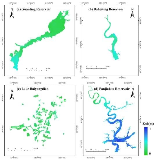
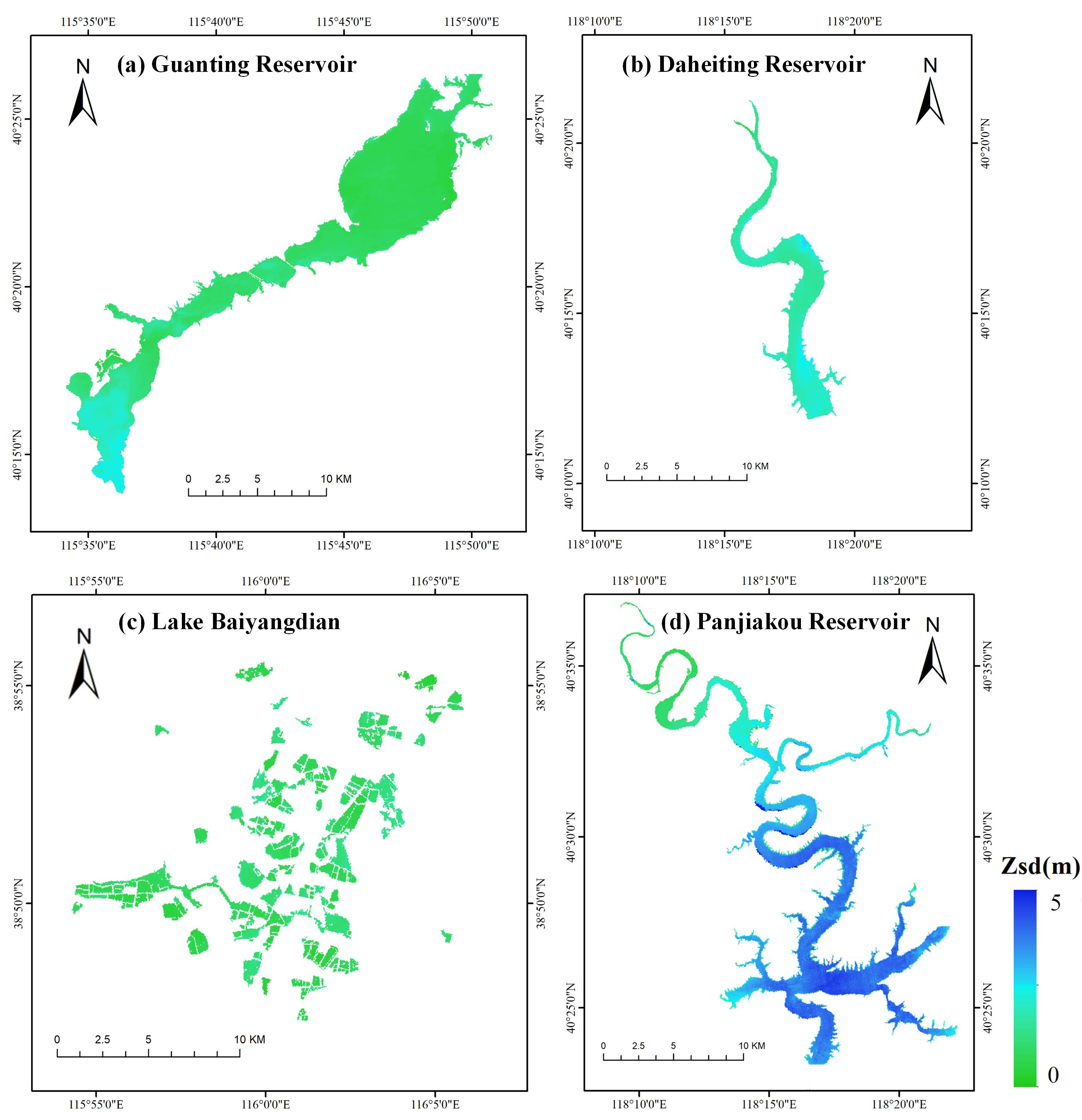
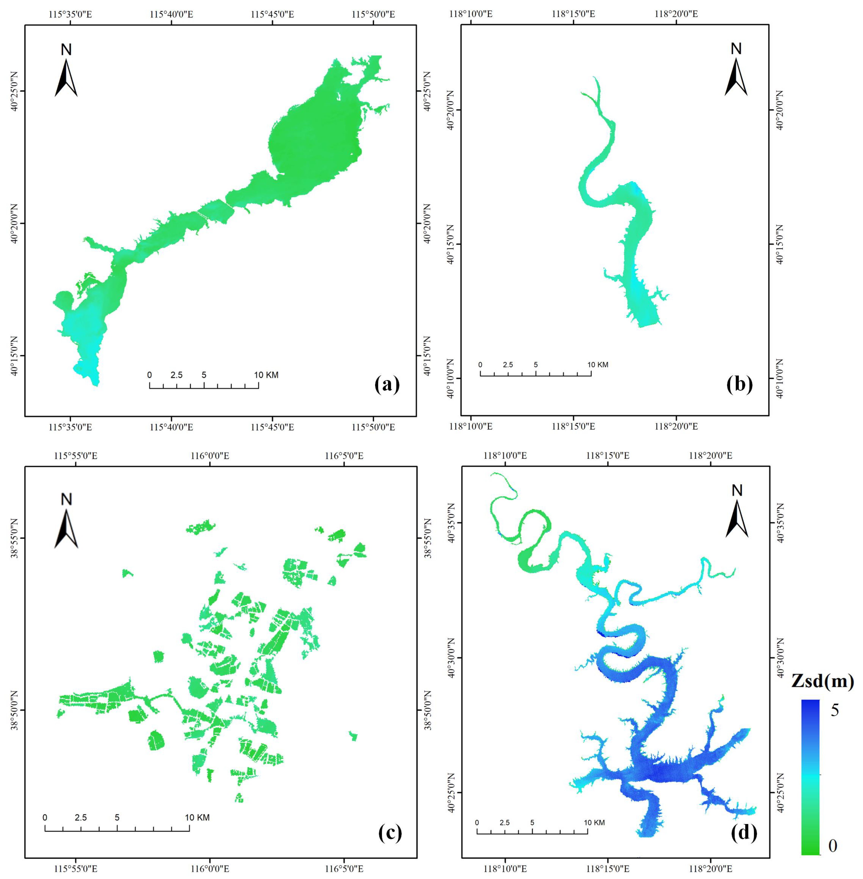
2.1. Study Areas and In Situ Measurements

Four inland lakes and reservoirs, including the Guanting Reservoir, Baiyangdian Lake, Panjiakou Reservoir and Daheiting Reservoir in the Hebei Province of China are selected as the study areas. In situ experiments were implemented to acquire match-up measurements of the GF-5 satellite (Figure 1). Guanting Reservoir is located in Huailai county with an area of 130 km${}^2$, which serves as one of the standby drinking water sources for Beijing. Baiyangdian Lake, the largest lake in North China, is situated in the Xiong’an New Area. Panjiakou Reservoir is located at the junction of Tangshan city and Chengde district, while Daheiting Reservoir is 30 km downstream of Panjiakou Reservoir.

Table 1. Waterbody names, the central longitude and latitude of the study areas, in situ data acquisition date, number of samplings (N), and $Z_{sd}$ values for the field measurements.

No.	Study Region	Longitude	Latitude	In Situ Data	N	${\mathit{Z}}_{\mathit{sd}}$ (m)
				Acquisition Date		Mean	Min	Max
1	Guanting Reservoir	115.73 E	40.35 N	5/22/2019	18	1.16	0.30	2.15
2	Lake Baiyangdian	116.01 E	38.82 N	5/21/2019	16	1.13	0.70	1.60
				5/22/2019	13	1.13	0.55	1.70
3	Panjiakou Reservoir	118.29 E	40.43 N	9/24/2019	25	3.41	1.20	4.50
4	Daheiting Reservoir	118.31 E	40.28 N	9/25/2019	12	1.38	0.85	2.10

lists the basic information for the collected in situ measurements of the study regions.

The $Z_{sd}$ values at the sampling sites were measured using a standard 30-cm diameter Secchi disk. Water surface spectra were collected with a FieldSpec HandHeld ASD spectroradiometer according to the above-water method [22,23,24], simultaneously with the $Z_{sd}$ measurement. The water surface radiance ($L_u\left(\lambda \right)$), as well as the downwelling radiance ($L_d\left(\lambda \right)$) and skylight radiance ($L_{sky}\left(\lambda \right)$) were measured using the ASD spectroradiometer in the range from 400–900 nm at 1-nm intervals. For the $L_u\left(\lambda \right)$ measurement, the viewing zenith angle was 40${}^{\circ }$ downward, and the azimuth angle was 135${}^{\circ }$ away from the sun’s azimuth; for the $L_{sky}\left(\lambda \right)$ measurement, the viewing zenith angle was 40${}^{\circ }$ upward, and the azimuth angle was the same as the $L_u\left(\lambda \right)$ measurement. To acquire the $L_u\left(\lambda \right)$, the ASD spectroradiometer was targeted vertically over a reference panel center to measure its reflected radiance $L_p\left(\lambda \right)$ at a zenith angle of 0${}^{\circ }$, and the $L_u\left(\lambda \right)$ were then calculated as $L_p\left(\lambda \right)/{\rho }_p$.

For each sampling site, we conducted spectra measurement in the following order: (1) five measures of $L_d\left(\lambda \right)$, (2) ten measures of $L_u\left(\lambda \right)$, (3) five measures of $L_{sky}\left(\lambda \right)$, and (4) five measures of $L_d\left(\lambda \right)$. As the single-channel-based above-water method requires stable sunlight, the difference among the five $L_u\left(\lambda \right)$ measurements cannot exceed 10% in both steps 1 and 4, and so does for the difference between averaged-$L_d\left(\lambda \right)$ in step 1 and 4. Measurements not meeting these criteria were discarded. In addition, for $L_u\left(\lambda \right)$, we check if unusually large spectra existed in the ten measurements. Unusually large spectra occur possibly due to random solar flares, and were discarded. The average of the remaining spectrum was then taken.

The above-water remote sensing reflectance ($R_{rs}$) was then calculated as follows:

$$\begin{array}{c}\hfill R_{rs}\left(\lambda \right)=\frac{L_u\left(\lambda \right)-{\rho }_{sky}\left(\lambda \right)L_{sky}\left(\lambda \right)}{\pi L_p/{\rho }_p},\end{array}$$

(1)

where ${\rho }_p$ is the reflectance of the reference panel calibrated in the laboratory; and ${\rho }_{sky}$ is the skylight reflectance determined from the look-up table in Reference [25]. ${\rho }_{sky}$ is affected by the wind speed, solar zenith angle, and the viewing geometry, and is thought to be independent of the wavelength. Though some studies [26,27] propose sophisticated approaches to compute ${\rho }_{sky}$ considering the spectral variations of skylight distribution, we choose the method in Reference [25], as it is widely used and easy to implement. Moreover, the error in $R_{rs}$ caused by small residual errors in ${\rho }_{sky}$ mainly exists in the dark blue wavelengths, and is smaller for turbid waters. Figure 2 shows the in situ collected $R_{rs}$ in the study areas.

2.2. Satellite Data Acquisition and Preprocessing

We included four AHSI images that have match-up in situ measurements with these study regions. Images of Guanting Reservoir and Baiyang Lake were collected on 22 May 2019, while images for the Panjiakou and Daheiting Reservoirs were acquired on 24 September 2019. All images were acquired at approximately 1 p.m. local time. For the in situ experiment, all field data at Guanting and Panjiakou Reservoirs were acquired within 3 h of the overpass time; but 16 of the 29 samples collected from Lake Baiyangdian and all 12 samples from Daheiting Reservoir were measured one day before and after GF-5 overpass, respectively.

Before $Z_{sd}$ estimation, the DN values from the original AHSI data should be corrected to $R_{rs}$, and water areas must be extracted. All scenes were corrected using the FLAASH module in the ENVI5.3 software. Specifically, the VNIR and SWIR images were first merged into one file due to separate storage. Second, DN values were rescaled to top-of-atmosphere radiance using the radiometric calibration coefficients in the metadata file. Third, surface reflectance ($\rho$) images were retrieved from the FLAASH module. We used the rural aerosol model in FLAASH for all AHSI images, since aerosols in the study areas were not strongly affected by urban or industrial sources. In addition, we chose the 2-band Kaufman-Tanre aerosol retrieval method (called 2-band (K-T) in the FLAASH interface). The 2-band (K-T) method is based on detecting forested or dense vegetation pixels as the darkest pixels over the land [28]. Since dense vegetation has relatively high reflectance that can be accurately calibrated in AHSI images, it is reasonable to apply the 2-band (K-T) method in AHSI atmospheric correction. A final remaining problem is the retrieval of $R_{rs}$ from $\rho$. According to Equation (1), $\rho$ is related to $R_{rs}$ as follows:

$$\begin{array}{cc}\hfill R_{rs}\left(\lambda \right)& =\frac{L_u\left(\lambda \right)}{\pi L_d\left(\lambda \right)}-\frac{{\rho }_{sky}\left(\lambda \right)L_{sky}\left(\lambda \right)}{\pi L_d\left(\lambda \right)}\hfill \\ \hfill & =\frac{\rho \left(\lambda \right)}{\pi }-\frac{{\rho }_{sky}\left(\lambda \right)L_{sky}\left(\lambda \right)}{\pi L_d\left(\lambda \right)},\hfill \end{array}$$

(2)

where $L_d$ is the downwelling radiance on the water surface. Here, the skylight effects involved in the surface reflectance should be removed for accurate $R_{rs}$ retrieval. However, as the AHSI radiometric calibration parameters were acquired based on bright land targets [21], the SWIR band data contain a relatively high level of noise and thus cannot be applied for skylight removal of water bodies. Therefore, $R_{rs}$ is approximately represented as $\rho /\pi$ in the AHSI images (hereafter referred to as $R_{rs}^0$), neglecting skylight effects.

For the water area delineation, the Normalized Difference Water Index (NDWI) was calculated using surface reflectance $\rho$ followed by the application of the modified histogram bimodal method (MHBM) [29] to NDWI images to automatically segment water areas from other land cover types.

3. Secchi Disk Depth Estimation Method

This study aims to validate the application of AHSI data for inland water clarity monitoring, as well as the validation of the accuracy of SAM for use in the routine $Z_{sd}$ image production of AHSI imagery. Considering the complex optical properties of inland water in China, the semi-analytical model developed by Lee et al. [16] was selected and tested for the $Z_{sd}$ of the AHSI imagery. This algorithm can be applied to hyperspectral or MODIS and SeaWiFS sensors, and has been modified to be successfully applied to Landsat-8 imagery [30]. There are three major steps required to retrieve $Z_{sd}$ with the semi-analytical model: (1) estimate the inherent optical properties (IOPs), that is, the total absorption coefficient, a, and backscattering coefficient, $b_b$; (2) retrieve the diffuse attenuation coefficient ($K_d$, $m^{-1}$) based on a and $b_b$; and (3) determine $Z_{sd}$ with $K_d$ and $R_{rs}$. These three steps are explained in the following sections.

3.1. IOPs Estimation Using the QAA Method

Lee et al. [17] developed a multi-band QAA algorithm to retrieve the absorption and backscattering coefficients from $R_{rs}$. QAA has six steps, including analytical and empirical approaches. Originally proposed and applied in optically deep waters, this method has received certain modifications to achieve better performance in turbid inland waters [31,32,33]. These modifications mainly include shifting the reference band to longer wavelengths and the alteration of the empirical equation in the algorithm.

Table 2. Steps to derive the absorption and backscattering coefficients from $QA{A}_{V5}$, $QA{A}_{L09}$ and $QA{A}_{M14}$.

Step	Property	${\mathit{QAA}}_{\mathit{V}5}$	${\mathit{QAA}}_{\mathit{L}09}$	${\mathit{QAA}}_{\mathit{M}14}$
0	$r_{rs}$	$=R_{rs}/(0.52+1.7R_{rs})$${}^1$	same as $QA{A}_{V5}$	same as $QA{A}_{V5}$
1	$u\left(\lambda \right)$	$=\frac{-g_0+\sqrt{g_0^2+4g_1{r}_{rs}\left(\lambda \right)}}{2g_1}$	same as $QA{A}_{V5}$	same as $QA{A}_{V5}$
		$g_0=0.089g_1=0.125$
2	$a\left({\lambda }_0\right)$	$=a_w\left({\lambda }_0\right)+{10}^{-1.146-1.366\chi -0.469{\chi }^2}$	$=a_w\left({\lambda }_0\right)$	$=a_w\left({\lambda }_0\right)+{10}^{-0.7153-2.054\chi -1.047{\chi }^2}$
		$\chi =log\left(\frac{r_{rs}\left(443\right)+r_{rs}\left(490\right)}{r_{rs}\left({\lambda }_0\right)+5\frac{r_{rs}\left(667\right)}{r_{rs}\left(490\right)}{r}_{rs}\left(667\right)}\right)$		$\chi =log\left(\frac{0.01r_{rs}\left(443\right)+r_{rs}\left(620\right)}{r_{rs}\left({\lambda }_0\right)+0.005\frac{r_{rs}\left(620\right)}{r_{rs}\left(443\right)}{r}_{rs}\left(620\right)}\right)$
		${\lambda }_0=555$	${\lambda }_0=710$	${\lambda }_0=708$
3	$b_{bp}\left({\lambda }_0\right)$	$=\frac{u\left({\lambda }_0\right)a\left({\lambda }_0\right)}{1-u\left({\lambda }_0\right)}-b_{bw}\left({\lambda }_0\right)$	$=\frac{u\left({\lambda }_0\right)a\left({\lambda }_0\right)}{1-u\left({\lambda }_0\right)}$	same as $QA{A}_{V5}$
4	$\eta$	$=2.0\left\{1-1.2exp\left[-0.9\frac{r_{rs}\left(443\right)}{r_{rs}\left(555\right)}\right]\right\}$	$=2.2\left\{1-1.2exp\left[-0.9\frac{r_{rs}\left(560\right)}{r_{rs}\left(750\right)}\right]\right\}$	same as $QA{A}_{V5}$
5	$b_{bp}\left(\lambda \right)$	$=b_{bp}\left({\lambda }_0\right){\left(\frac{{\lambda }_0}{\lambda }\right)}^{\eta }$	same as $QA{A}_{V5}$	same as $QA{A}_{V5}$
6	$a\left(\lambda \right)$	$=\frac{[1-u\left(\lambda \right)][b_{bp}\left(\lambda \right)+b_{bw}\left(\lambda \right)]}{u\left(\lambda \right)}$	same as $QA{A}_{V5}$	same as $QA{A}_{V5}$

${}^1$$R_{rs}$: above-surface remote-sensing reflectance, $r_{rs}$: below-surface remote-sensing reflectance, $u\left(\lambda \right)$: ratio of the backscattering coefficient to the sum of the absorption and backscattering coefficients ($b_b/(a+b_b$), ${\lambda }_0$: reference wavelength, $\eta$: spectral power of the particle scattering coefficient.

lists the steps of the fifth version of the QAA ($QA{A}_{V5}$), with modified QAA algorithm steps for turbid waters, referred to as $QA{A}_{L09}$ [31] and $QA{A}_{M14}$ [32], respectively. $QA{A}_{L09}$ uses 710 nm as its reference wavelength, at which point neglects the absorption of suspended solids and phytoplankton, where $a\left(710\right)$ is approximately equal to $a_w\left(710\right)$. The pure-water backscattering coefficient $b_{bw}\left(710\right)$ was also neglected in the $b_{bp}\left(710\right)$ calculation. In addition, the $r_{rs}$ wavelengths were assessed, with a selection of 560 and 750 nm. $QA{A}_{M14}$ used 708 nm as the reference wavelength, obtaining a new empirical relationship between $a\left(710\right)$ and $\chi$, which is an intermediate parameter for the derivation of $a\left(710\right)$ and calculated using a new equation based on the $r_{rs}$ at 443 and 620 nm.

In addition, QAA was updated to its sixth version ($QA{A}_{V6}$). In the $QA{A}_{V6}$ algorithm, the same steps in $QA{A}_{V5}$ [34] were used for both a and $b_{bp}$ estimation when $R_{rs}$ was less than 0.0015 $s{r}^{-1}$. Otherwise, the reference wavelength (${\lambda }_0$) is shifted to 670 nm, where $a\left({\lambda }_0\right)$ can be calculated using a different equation:

$$a\left({\lambda }_0\right)=a\left(670\right)=a_w\left(670\right)+0.39{\left(\frac{R_{rs}\left(670\right)}{R_{rs}\left(443\right)+R_{rs}\left(490\right)}\right)}^{1.14},$$

(3)

where $a_w$ is the absorption coefficient of pure water. In Section 4, we tested $QA{A}_{V5}$, $QA{A}_{V6}$, $QA{A}_{L09}$ and $QA{A}_{M14}$ on the AHSI band-equivalent in situ $R_{rs}$ for $Z_{sd}$ determination.

3.2. $K_d$ Retrieval Using IOPs

According to the radiative transfer theory, the diffuse attenuation coefficient, $K_d$, can be expressed as an analytical function of a and $b_b$. Lee et al. [35] updated the semi-analytical model of $K_d$ as follows:

$$K_d\left(\lambda \right)=(1+m_0\times {\theta }_s)a\left(\lambda \right)+(1-\gamma \frac{b_{bw}\left(\lambda \right)}{b_b\left(\lambda \right)})\times m_1\times (1-m_2\times e^{-m_3\times a\left(\lambda \right)})b_b\left(\lambda \right),$$

(4)

where $\lambda$ is the wavelength; ${\theta }_s$ is the solar zenith angle in degrees; $b_{bw}\left(\lambda \right)$ is the backscattering coefficient of pure water; $m_{0-3}$ and $\gamma$ are parameters with fixed values of 0.005, 4.26, 0.52, 10.8, and 0.265, respectively. Both $a\left(\lambda \right)$ and $b_b\left(\lambda \right)$ are retrieved from the QAA.

3.3. $Z_{sd}$ Estimation Based on $K_d$ and $R_{rs}$

The classic underwater visibility theory interprets that the $Z_{sd}$ is inversely proportional to the sum of the diffuse attenuation and beam attenuation coefficients (c, m${}^{-1}$) [36]. As c is generally 2–5-fold greater than $K_d$, this theory contradicts the fact that no universal connections exist between $Z_{sd}$ and c, which is corroborated by human experience with respect to the Secchi disk depth. To solve these problems, Lee et al. [16] developed a new underwater visibility theory, arguing that $Z_{sd}$ is only inversely proportional to $K_d$ and can be expressed as follows:

$$Z_{sd}=\frac{1}{2.5min\left(K_d^{tr}\right)}ln\left(\frac{|0.14-R_{rs}^{tr}|}{0.013}\right),$$

(5)

where $K_d^{tr}$ denotes the diffuse attenuation coefficient of the water body over the visible spectral range (410–665 nm), and $R_{rs}^{tr}$ represents the corresponding remote-sensing reflectance at this wavelength. Specifically, we must retrieve the $K_d$ at 443, 488, 532, 555, and 665 nm.

3.4. Accuracy Assessment Method

The performance of the semi-analytical models based on $QA{A}_{V5}$, $QA{A}_{V6}$, $QA{A}_{L09}$ and $QA{A}_{M14}$ was first evaluated using the AHSI band-equivalent in situ $R_{rs}$ datasets. The $Z_{sd}$ values derived from these models were compared with the in situ measured $Z_{sd}$. The mean absolute error (MAE), mean relative error (MRE), and coefficient of determination ($R^2$) values were calculated to assess the accuracy of these semi-analytical models applied to the AHSI $R_{rs}$. Furthermore, semi-analytical models that have achieved good performance using in situ spectra were then selected for implementation with the AHSI image $R_{rs}$. As with the in situ datasets, the MAE, MRE and $R^2$ of the image-retrieved $Z_{sd}$ values were used to assess these semi-analytical models applied to the AHSI data, as well as for an evaluation of the AHSI’s ability for inland water clarity monitoring.

4. Results

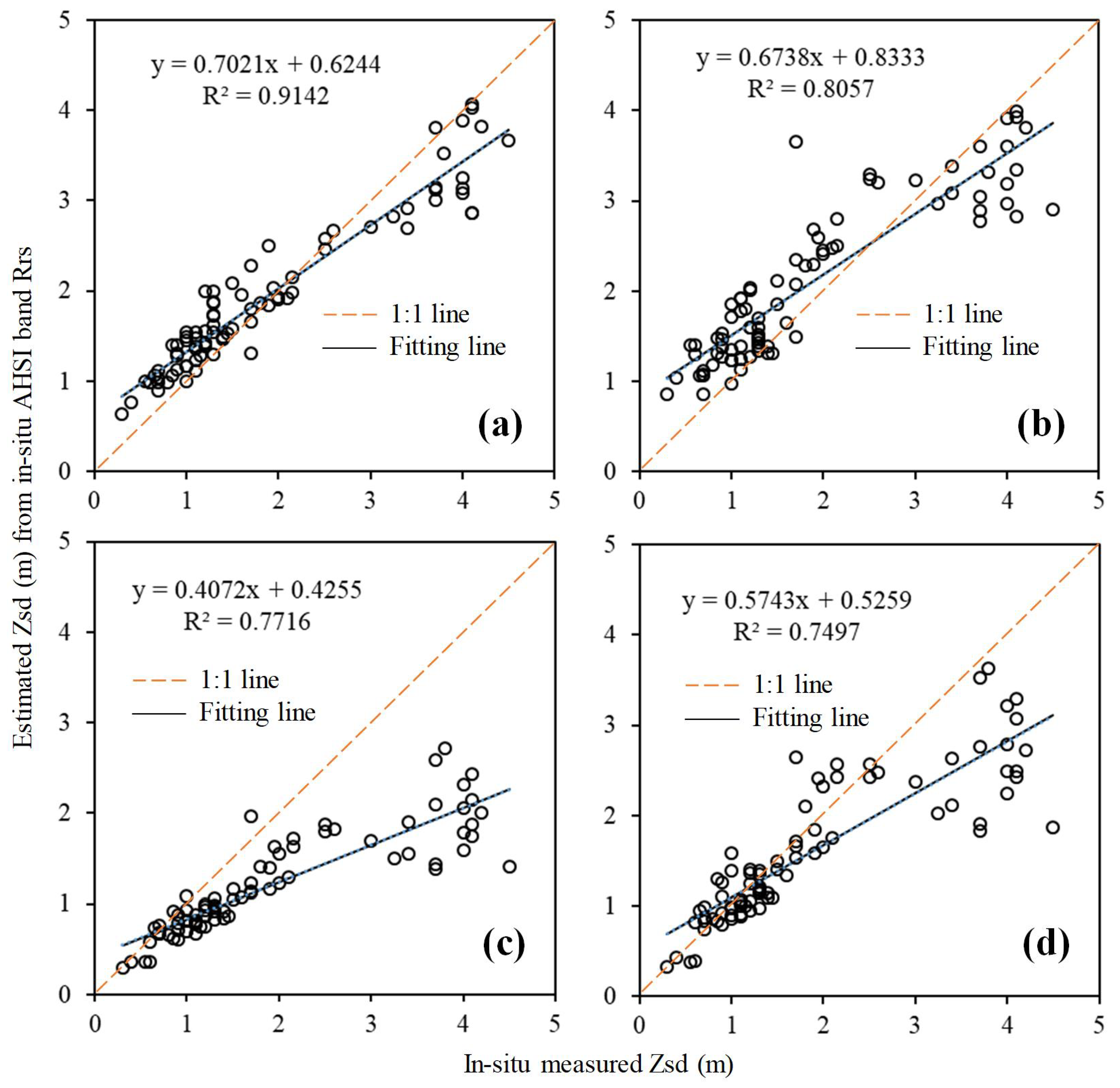
4.1. $Z_{sd}$ Estimation from In Situ Measurements

We first calculated the band-equivalent AHSI reflectance using field-measured $R_{rs}$. Following the steps in Section 3.3, the AHSI bands that have the most similar center wavelengths to the bands listed in Table 2 and Equation (3) were selected to calculate the $Z_{sd}$. Then, the MAEs of the derived $Z_{sd}$ were calculated, as well as the linear correlation analysis conducted between the estimated and measured $Z_{sd}$ values for all sampling points. The estimated $Z_{sd}$ values yielded MAE values of 0.35, 0.48, 0.69, and 0.42 m from SAMs based on $QA{A}_{V5}$, $QA{A}_{V6}$, $QA{A}_{L09}$, and $QA{A}_{M14}$, respectively. Figure 3 shows the estimation results with the in situ measured $Z_{sd}$ values.

Table 3. The MAEs and MREs of the estimated $Z_{sd}$ from the AHSI in situ $R_{rs}$ based on the semi-analytical methods using various QAA algorithms. Optimal results listed in bold.

	${\mathit{Z}}_{\mathit{sd}}$ Range (m)	N	${\mathit{QAA}}_{\mathit{V}5}$	${\mathit{QAA}}_{\mathit{V}6}$	${\mathit{QAA}}_{\mathit{L}09}$	${\mathit{QAA}}_{\mathit{M}14}$
MAE (m)	0.3–1.0	23	0.34	0.49	0.13	0.18
	1.0–3.0	43	0.25	0.44	0.46	0.21
	>3.0	18	0.57	0.56	1.96	1.26
	0.3–4.5	84	0.35	0.48	0.69	0.42
MRE	0.3–1.0	23	48.4%	72.1%	15.5%	22.8%
	1.0–3.0	43	18.2%	28.7%	28.7%	12.8%
	>3.0	18	14.7%	14.2%	50.3%	32.3%
	0.3–4.5	84	25.7%	37.5%	29.7%	19.7%

lists the MAEs and MREs for different $Z_{sd}$ ranges.

As shown in Figure 3, the $Z_{sd}$ values retrieved with $QA{A}_{V5}$ (Figure 3a) and $QA{A}_{V6}$ (Figure 3b) show better consistency with the in situ measurements, as their paired data in the study regions predominantly fall along a 1:1 line, also yielding a higher $R^2$ value (i.e., 0.9142 and 0.8057, respectively). The estimated $Z_{sd}$ using the modified $QA{A}_{L09}$ and $QA{A}_{M14}$ are characterized by weaker correlations with the field-measured $Z_{sd}$ ($R^2$ of 0.7716 and 0.7497, respectively). In addition, as shown by Figure 3c,d, the semi-analytical methods with $QA{A}_{L09}$ and $QA{A}_{M14}$ tend to underestimate the $Z_{sd}$ for relatively clear waters.

Based on Table 3, we can observe the performance of the $Z_{sd}$ estimations using the different QAA methods in various clarity ranges:

(1) Overall, the $QA{A}_{V5}$ and $QA{A}_{M14}$ yield desirable estimations with both small MAEs and MREs for the $Z_{sd}$ at all sampling sites. Specifically, $QA{A}_{V5}$ yields better predictions in clearer waters (i.e., $Z_{sd}$ > 3 m), whereas $QA{A}_{M14}$ performs better for more turbid waters ($Z_{sd}$ between 0.3 and 3 m). In addition, for a $Z_{sd}$ range from 1–3 m, both the MAEs and MREs of the $Z_{sd}$ estimated using the $QA{A}_{V5}$ are slightly bigger than those of the $Z_{sd}$ estimated from the $QA{A}_{M14}$.

(2) On the other hand, $QA{A}_{V6}$ and $QA{A}_{L09}$ have limitations for $Z_{sd}$ retrieval using AHSI data. Their overall MAEs and MREs are higher than the $Z_{sd}$ determined from two other algorithms. $QA{A}_{V6}$ tends to better estimate the $Z_{sd}$ for clearer waters (>3 m) and can induce larger errors in turbid areas (0.3–1 m). The opposite is true for $Z_{sd}$ values derived using the $QA{A}_{L09}$ method.

Taking into account the MAE, MRE, and correlation from the estimated $Z_{sd}$ values using the in situ dataset, we selected the $QA{A}_{V5}$- and $QA{A}_{M14}$-based semi-analytical methods for AHSI image testing.

4.2. $Z_{sd}$ Estimation Scheme for AHSI Imagery

Semi-analytical methods with $QA{A}_{V5}$ and $QA{A}_{M14}$ were both tested with the match-up pixels of the in situ sampling points using the image $R_{rs}^0$ described in Section 2.2. Figure 4 shows scatterplots of estimated and in situ measured $Z_{sd}$ with their corresponding $R^2$ values. As shown in Figure 4, the $Z_{sd}$ values generated from the $QA{A}_{V5}$-based method have a significantly higher correlation and better consistency with the in situ measurements than the SAM incorporating the $QA{A}_{M14}$ algorithm. An accuracy analysis (the same as in Section 4.1) was conducted for the imaged $Z_{sd}$ estimations.

Table 4. Mean absolute errors (MAEs) and mean relative errors (MREs) of the estimated Advanced HyperSpectral Imager (AHSI) image $Z_{sd}$ based on semi-analytical methods using various Quasi-Analytical Algorithm (QAA) algorithms. Optimal results listed in bold.

${\mathit{Z}}_{\mathit{sd}}$ Range (m)	N	MAE (m)		MRE
		${\mathit{QAA}}_{\mathit{V}\mathbf{5}}$	${\mathit{QAA}}_{\mathit{M}\mathbf{14}}$	${\mathit{QAA}}_{\mathit{V}\mathbf{5}}$	${\mathit{QAA}}_{\mathit{M}\mathbf{14}}$
0.3–1.0	23	0.22	0.39	33.1%	47.4%
1.0–3.0	43	0.46	0.98	29.1%	60.9%
>3.0	18	0.24	2.94	6.3%	75.6%
Total	84	0.35	1.24	25.3%	60.4%

lists the MAEs and MREs of 84 match-up pixels at different clarity ranges based on different methods using the AHSI image-estimated remote sensing reflectance. Only the $Z_{sd}$ determined from the $QA{A}_{V5}$-based semi-analytical method is acceptable for the AHSI data. For the 84 match-up measurements, the $Z_{sd}$ calculated with the $QA{A}_{V5}$ using $R_{rs}^0$ yields higher accuracy in terms of both the MAE and MRE. The $QA{A}_{V5}$-derived image $Z_{sd}$ is also more accurate than the $QA{A}_{M14}$ for $Z_{sd}$ at all ranges.

Furthermore, we compared the accuracies of image-derived $Z_{sd}$ based on MAE, MRE and $R^2$ (see

Table 5. AHSI image-derived $Z_{sd}$ accuracies for the 56 samples collected on the same day as the image acquisition, and 28 collected before/after one day.

Time Difference between	${\mathit{Z}}_{\mathit{sd}}$ Range (m)	N	MAE (m)	MRE	${\mathit{R}}^2$
In Situ Data and AHSI Image
Within 3 h	0.3–4.5	56	0.38	26.1%	0.871
Before/after 1 day	0.7–2.1	28	0.28	23.7%	0.502

) of in situ samples collected within 3 h and before/after 1 day of the AHSI image acquisition (see Table 1). From Table 5, it can be observed that:

(1)

Samples collected within 3 h and before/after 1 day both yielded $Z_{sd}$ with high accuracies on the AHSI images, which is likely owing to the stable weather conditions (i.e., no strong wind or rainfall) during the image acquisition and in situ measurement.

(2)

The $R^2$ from the samples collected within 3 h is higher than that the other group, indicating that the image-retrieved $Z_{sd}$ has better consistency with the in situ $Z_{sd}$ measured on the same day.

(3)

Samples collected before/after 1 day have smaller MAE and MRE than those collected on the same day. This is because highly turbid sampling sites (i.e., $Z_{sd}$ < 0.7 m) included in the latter have worse $Z_{sd}$ predictions, leading to greater MAE and MRE in this group of samples.

All of the above analyses indicate that only the SAM with the $QA{A}_{V5}$ can predict desirable $Z_{sd}$ values with an approximate remote sensing reflectance from the AHSI imagery. Therefore, based on the semi-analytical method with the $QA{A}_{V5}$, $Z_{sd}$ images were produced for the AHSI images of four study areas (see Figure 5). Retrieved $Z_{sd}$ from the study regions have consistent distributions with ground surveys: (1) in Guanting Reservoir, southwestern areas have higher water clarity than northeastern areas; (2) Lake Baiyangdian contains numerous small fish ponds, which have relative turbid waters in its most areas; and (3) Panjiakou Reservoir has better water quality than Daheiting Reservoir, such that it has higher water clarities.

5. Discussion

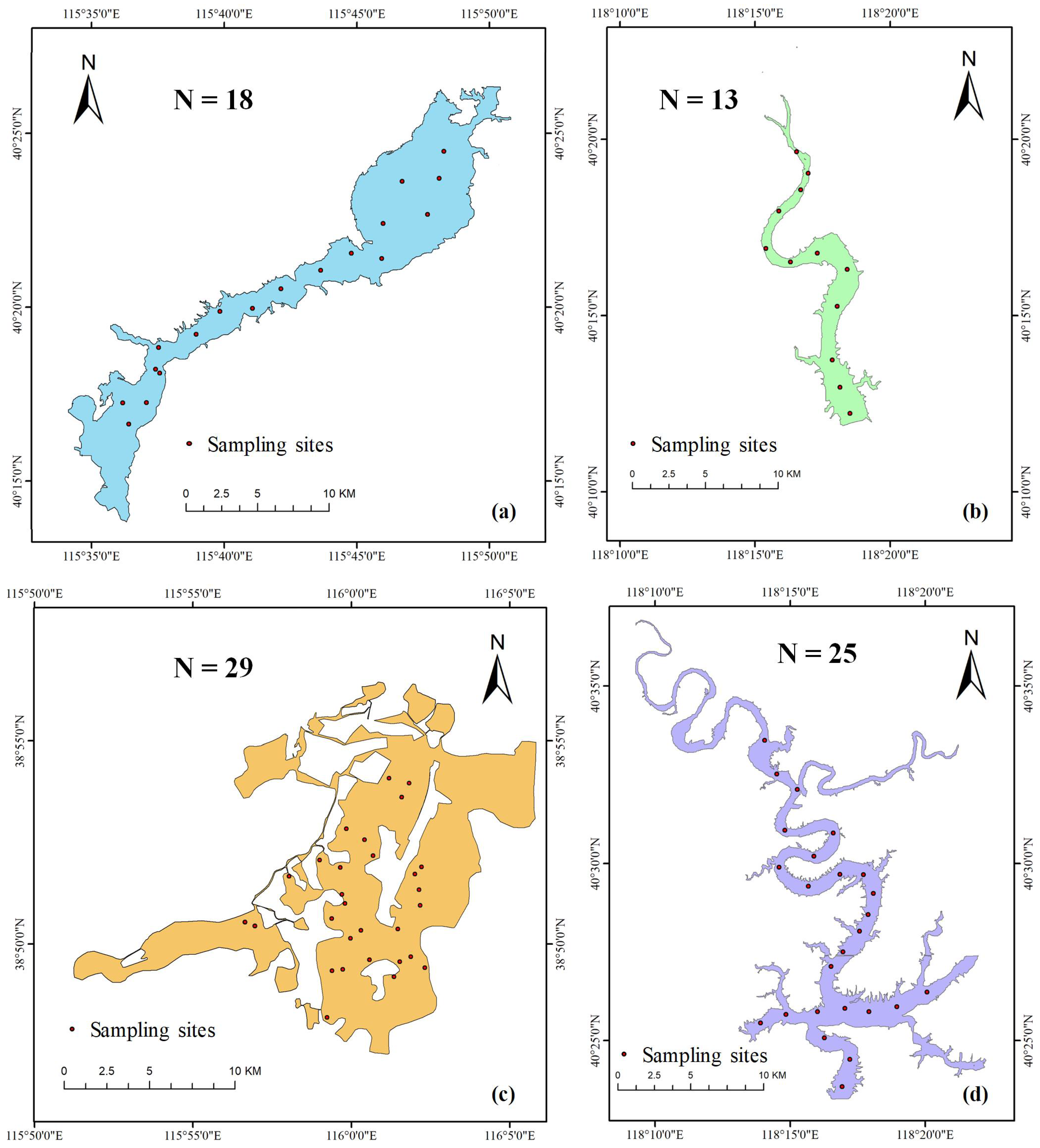
5.1. AHSI Atmospheric Correction Performance Evaluation

As the image $Z_{sd}$ is retrieved based on the $R_{rs}^0$, we made a comparison between the image $R_{rs}^0$ and the in situ $R_{rs}$ for the evaluation of the AHSI atmospheric correction results. $R_{rs}^0$ and in situ $R_{rs}$ of typical samples are shown in the Figure 6, and the average $R^2$ of all the 84 samples is 0.860 between $R_{rs}^0$ and $R_{rs}$ in the bands utilized in the QAA algorithms. Figure 6 shows that the $R_{rs}^0$ retrieved from AHSI images are generally slightly higher than the in-situ measured $R_{rs}$, but their spectral shapes are very similar. Since the $R_{rs}^0$ does not have skylight removal and is atmospherically corrected without accurate aerosol retrieval, the value of $R_{rs}^0$ on the AHSI image are considered as reasonable.

5.2. $Z_{sd}$ Estimation Methods Evaluation

Based on the $Z_{sd}$ values estimated from the AHSI band in situ $R_{rs}$, we can observe that the SAMs based on the $QA{A}_{V6}$ and $QA{A}_{L09}$ are unable to provide satisfactory predictions. In contrast, the SAMs with $QA{A}_{V5}$ and $QA{A}_{M14}$ gives good estimations for $Z_{sd}$ from the in situ measured spectra. Therefore, we applied the $QA{A}_{V5}$- and $QA{A}_{M14}$-based SAMs to the AHSI $R_{rs}$ images. Only $QA{A}_{V5}$ can generate $Z_{sd}$ with high accuracy from the AHSI data. The application of these SAMs to AHSI imagery were evaluated as follows.

(1)

$QA{A}_{V6}$-based SAM evaluation

Based on the in situ acquired AHSI $R_{rs}$, $QA{A}_{V6}$ yielded good predictions only for $Z_{sd}$ values higher than 3.0 m due to its limitations in turbid water. In addition, the semi-analytical method with $QA{A}_{V6}$ was evaluated as being capable of retrieving the $Z_{sd}$ for an oligo- to mesotrophic inland reservoir [37], but acquired an average relative error of 75.05%.

(2)

$QA{A}_{L09}$-based SAM evaluation

$QA{A}_{L09}$ was developed with limited samples collected from Lake Taihu, with sensitivity to water contents and optical properties as mentioned in Reference [31]. Specifically, the $Z_{sd}$ range of Lake Taihu is 0–0.9 m, which is distinct from the water clarity range of our study regions. This is likely the reason for poor performance in terms of the $Z_{sd}$ retrieval in our study regions.

(3)

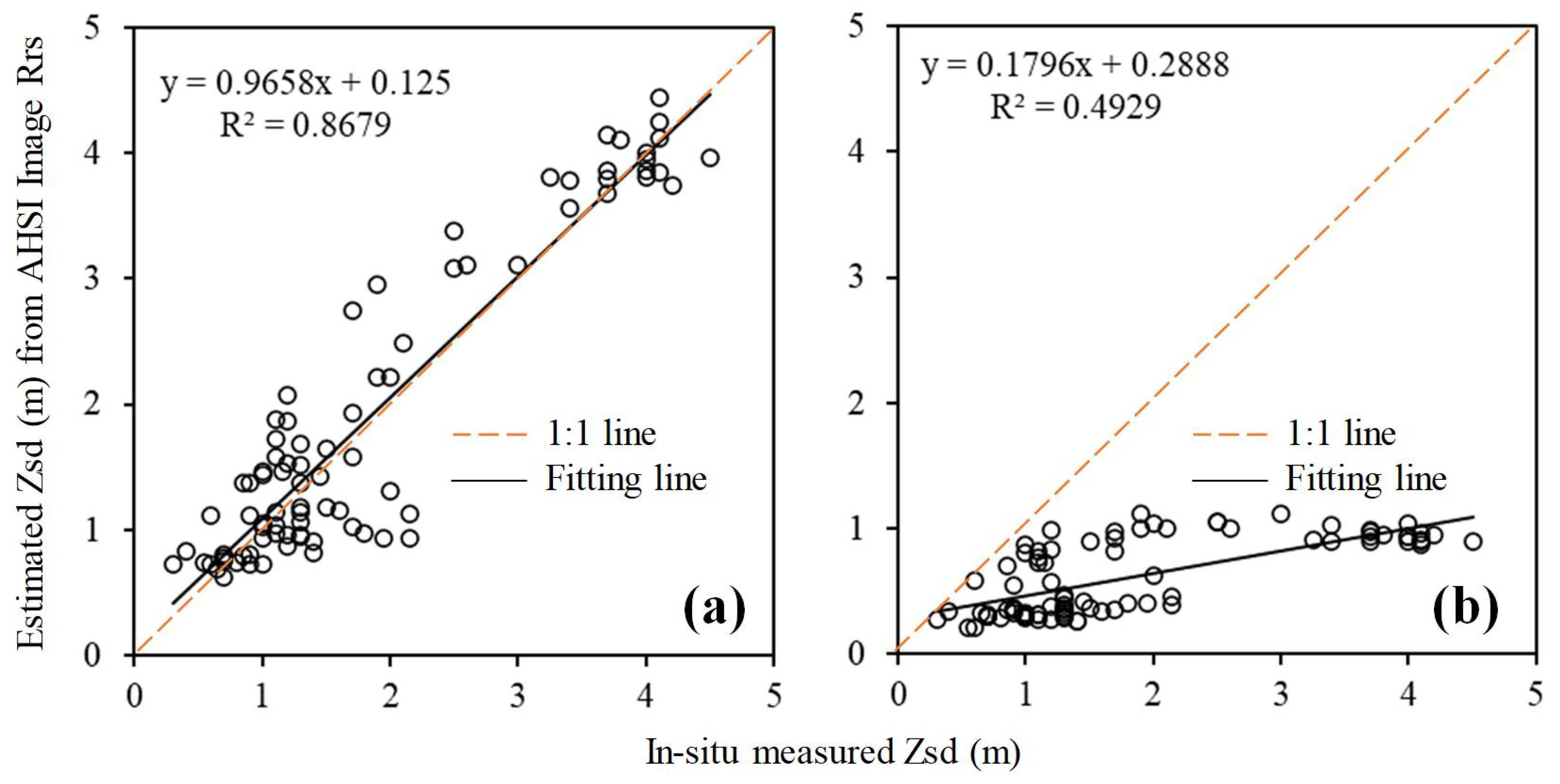
$QA{A}_{V5}$-based SAM evaluation

The estimated $Z_{sd}$ values based on the $QA{A}_{V5}$ using image $R_{rs}^0$ and AHSI in situ $R_{rs}$ have similar MAEs and MREs. In other words, the image $Z_{sd}$ with $R_{rs}^0$ is generally consistent with the AHSI in-situ $R_{rs}$ generated results when using the $QA{A}_{V5}$-based semi-analytical method, despite an approximated $R_{rs}^0$ for the image that is generally higher than the in situ measured reflectance due to insufficient atmospheric correction. Since $a\left(\lambda \right)$ and $b_b\left(\lambda \right)$ are mainly affected by the shape and magnitude of the $R_{rs}$, respectively [38], $a\left(\lambda \right)$ retrieved from the image is consistent with the in situ-derived values. In addition, $a\left(\lambda \right)$ affects $K_d$ and $Z_{sd}$ to a more extent than does $b_b\left(\lambda \right)$, and therefore, the image-retrieved $Z_{sd}$ values are comparable to the in situ-derived results. However, the estimation accuracies were different at various $Z_{sd}$ ranges between the image and in situ derived $Z_{sd}$. For the clarity range of 1–3 m, the estimated image $Z_{sd}$ has poorer accuracies (MRE of 29.1%) than the in situ determined $Z_{sd}$ (MRE of 18.2%). In contrast, the image-generated $Z_{sd}$ was better than that of the in situ values for <1 m and >3 m clarity conditions.

(4)

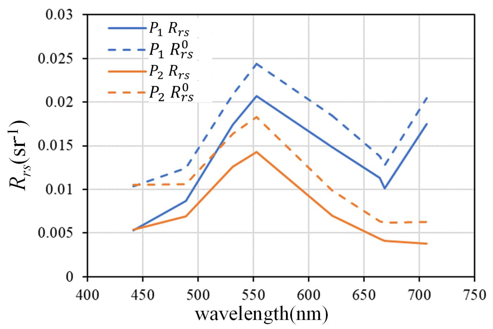
$QA{A}_{M14}$-based SAM evaluation

For the $QA{A}_{M14}$-based method, the image $R_{rs}^0$, however, acquired distinct $Z_{sd}$ results compared with those estimated from the AHSI band-equivalent in situ $R_{rs}$. Unlike the AHSI in situ $R_{rs}$ that generated desirable $Z_{sd}$ predictions using the $QA{A}_{M14}$, the $Z_{sd}$ values calculated from the image $R_{rs}^0$ have significantly poorer accuracies. Specifically, the MRE is 47.4% for a $Z_{sd}$ of less than 1 m, while the MRE increases to 60.9 and 75.6% for $Z_{sd}$ values ranging from 1–3 m and >3 m, respectively. Moreover, the absolute error also increases from 0.42 to 1.24 m. Such large errors are unacceptable when estimating the water clarity in ranges from 0.3 to 4.5 m. Figure 6 shows that image $R_{rs}^0$ is higher than in situ $R_{rs}$ but with similar spectral shapes. However, the ratio of image $R_{rs}^0$ and in-situ $R_{rs}$ at 708 nm is greater than that at 555 nm, since $R_{rs}$ is much lower in the 708 nm band. Therefore, the use of 708 nm in $QA{A}_{M14}$ algorithm leads to an overestimation of $b_b$ and $K_d$, which finally results in an underestimation for $Z_{sd}$ on AHSI images.

In addition to the above discussion, we discuss samples used in the development of semi-analytical methods applied in Section 4 from the available literature [16,31,32,34]. the $QA{A}_{V5}$ has been validated with the NOMAD dataset (>600 samples) [34], which has a wide range of $Z_{sd}$ values [16]. $QA{A}_{L09}$ was developed with 13 in situ measurements, and it exhibits good accuracy with a validation dataset of 33 samples [31]; The calibration and validation datasets for $QA{A}_{M14}$ contained 20 and 21 in situ measurement samples, respectively [32]. Therefore, $QA{A}_{V5}$ is likely to be more robust than other modified QAA algorithms.

5.3. Validation Limitations

The $Z_{sd}$ estimations were validated for the in situ dataset ranging from 0.3 to 4.5 m, with a lack of validations for highly turbid or clear waters. Considering that the semi-analytical method has been tested with $Z_{sd}$ values of 0.1–30 m in coastal and oceanic waters [16], we must further validate its applicability to AHSI data with more turbid waters (i.e., $Z_{sd}$ < 0.3 m) in the future.

5.4. GF-5 Applicability to $Z_{sd}$ Retrieval

The above experiments show the possibility of retrieving water clarity using GF-5 AHSI imagery. Compared with multispectral instruments (e.g., MODIS and MERIS), AHSI data has the following advantages for water clarity monitoring: (1) its high spectral resolution and continuous spectral range provides a selection of numerous bands; and (2) its spatial resolution is higher than most other instruments used for water monitoring, such that it can be used in small or medium-sized water bodies. In addition, as AHSI has the same spatial resolution as the Landsat series, its high spectral resolution may yield $Z_{sd}$ with higher accuracies. For example, the estimated $Z_{sd}$ using the $QA{A}_{V5}$-based SAM on the Landsat-8 imagery had MREs of 12.86%, 28.83%, and 31.17% for the Nav Reservoir in the in situ $Z_{sd}$ ranges of 2.29–4.80, 2.45–4.65, and 1.91–3.80 m, respectively [37]; the Ibitinga Reservoir received a MRE of 34.6% using the same method on the Landsat-8 image for a water clarity between 1.8–2.6 m [39]; and the MRE of derived $Z_{sd}$ from the Landsat-8 data was 64% for the Boston Harbor, which had a water clarity between 0.5 and 4 m [40]. For the comparable $Z_{sd}$ range (i.e., 0.3–4.5 m), AHSI achieved generally higher accuracy with a MRE of 25.3% despite its approximate $R_{rs}$ values.

However, the GF-5 satellite has a long revisit period due to its relatively narrow swath, which limits its implementation for dynamic monitoring. With planned launches of other hyperspectral satellites, a hyperspectral satellite constellation can be established to shorten the revisit time, thereby promoting the advantages of water clarity estimations using the GF-5 satellite, as well as monitoring for other water quality parameters.

6. Conclusions

The new generation Chinese hyperspectral imager AHSI on board the GF-5 satellite has the potential to retrieve accurate water clarity values, as it has continuous narrow spectral bands from 400–2500 $\mathsf{\mu }$m. Also, AHSI imagery is suitable for monitoring the lakes and reservoirs that are not very large, due to its relatively high spatial resolution. In this study, we tested the AHSI data for its ability to monitor inland water clarity, as well as a validation of the accuracy in terms of the semi-analytical methods used for the routine $Z_{sd}$ image production of AHSI imagery. Four inland lakes and reservoirs in China were selected as the study regions. Concurrent in situ measurements were conducted when AHSI had acquired images. An accuracy analysis of the retrieved $Z_{sd}$ from the AHSI images shows that only the semi-analytical method incorporating the $QA{A}_{V5}$ algorithm can yield relatively high accuracies. For 84 concurrent sampling sites in a $Z_{sd}$ range of 0.3–4.5 m, the MAE and MRE were 0.35 m and 25.3%, respectively. Experimental results also indicate that the AHSI has sufficient bands for the implementation of the semi-analytical method, which can achieve desirable $Z_{sd}$ estimations with roughly estimated $R_{rs}$ AHSI images. Although further validation is still required for highly turbid and clear waters, our results indicate that the AHSI is effective to retrieve accurate water clarity data at different levels of transparency.

References

- Le, C.; Zha, Y.; Li, Y.; Sun, D.; Lu, H.; Yin, B. Eutrophication of lake waters in China: Cost, causes, and control. Environ. Manag. 2010, 45, 662–668. [Google Scholar] [CrossRef] [PubMed]
- Zhang, K.; Shi, H.; Peng, J.; Wang, Y.; Xiong, X.; Wu, C.; Lam, P.K. Microplastic pollution in China’s inland water systems: A review of findings, methods, characteristics, effects, and management. Sci. Total Environ. 2018, 630, 1641–1653. [Google Scholar] [CrossRef] [PubMed]
- Behmel, S.; Damour, M.; Ludwig, R.; Rodriguez, M.J. Water quality monitoring strategies—A review and future perspectives. Sci. Total Environ. 2016, 571, 1312–1329. [Google Scholar] [CrossRef] [PubMed]
- Becker, R.H.; Sayers, M.; Dehm, D.; Shuchman, R.; Quintero, K.; Bosse, K.; Sawtell, R. Unmanned aerial system based spectroradiometer for monitoring harmful algal blooms: A new paradigm in water quality monitoring. J. Great Lakes Res. 2019, 45, 444–453. [Google Scholar] [CrossRef]
- Shi, K.; Zhang, Y.; Zhu, G.; Qin, B.; Pan, D. Deteriorating water clarity in shallow waters: Evidence from long term MODIS and in-situ observations. Int. J. Appl. Earth Obs. Geoinf. 2018, 68, 287–297. [Google Scholar] [CrossRef]
- Holmes, R.W. The Secchi disk in turbid coastal waters 1. Limnol. Oceanogr. 1970, 15, 688–694. [Google Scholar] [CrossRef]
- Boyce, D.G.; Lewis, M.; Worm, B. Integrating global chlorophyll data from 1890 to 2010. Limnol. Oceanogr. Methods 2012, 10, 840–852. [Google Scholar] [CrossRef]
- Swift, T.J.; Perez-Losada, J.; Schladow, S.G.; Reuter, J.E.; Jassby, A.D.; Goldman, C.R. Water clarity modeling in lake Tahoe: Linking suspended matter characteristics to Secchi depth. Aquat. Sci. 2006, 68, 1–15. [Google Scholar] [CrossRef]
- Doron, M.; Babin, M.; Hembise, O.; Mangin, A.; Garnesson, P. Ocean transparency from space: Validation of algorithms estimating Secchi depth using MERIS, MODIS and SeaWiFS data. Remote Sens. Environ. 2011, 115, 2986–3001. [Google Scholar] [CrossRef]
- Alikas, K.; Kratzer, S. Improved retrieval of Secchi depth for optically-complex waters using remote sensing data. Ecol. Indic. 2017, 77, 218–227. [Google Scholar] [CrossRef]
- Olmanson, L.G.; Bauer, M.E.; Brezonik, P.L. A 20-year Landsat water clarity census of Minnesota’s 10,000 lakes. Remote Sens. Environ. 2008, 112, 4086–4097. [Google Scholar] [CrossRef]
- McCullough, I.M.; Loftin, C.S.; Sader, S.A. Combining lake and watershed characteristics with Landsat TM data for remote estimation of regional lake clarity. Remote Sens. Environ. 2012, 123, 109–115. [Google Scholar] [CrossRef]
- Mancino, G.; Nolè, A.; Urbano, V.; Amato, M.; Ferrara, A. Assessing water quality by remote sensing in small lakes: The case study of Monticchio lakes in southern Italy. iFor.-Biogeosci. For. 2009, 2, 154. [Google Scholar] [CrossRef] [Green Version]
- Thiemann, S.; Kaufmann, H. Lake water quality monitoring using hyperspectral airborne data—A semiempirical multisensor and multitemporal approach for the Mecklenburg Lake District, Germany. Remote Sens. Environ. 2002, 81, 228–237. [Google Scholar] [CrossRef]
- Binding, C.E.; Greenberg, T.A.; Watson, S.B.; Rastin, S.; Gould, J. Long term water clarity changes in north America’s Great Lakes from multi-sensor satellite observations. Limnol. Oceanogr. 2015, 60, 1976–1995. [Google Scholar] [CrossRef]
- Lee, Z.; Shang, S.; Hu, C.; Du, K.; Weidemann, A.; Hou, W.; Lin, J.; Lin, G. Secchi disk depth: A new theory and mechanistic model for underwater visibility. Remote Sens. Environ. 2015, 169, 139–149. [Google Scholar] [CrossRef] [Green Version]
- Lee, Z.; Carder, K.L.; Arnone, R.A. Deriving inherent optical properties from water color: A multiband quasi-analytical algorithm for optically deep waters. Appl. Opt. 2002, 41, 5755–5772. [Google Scholar] [CrossRef]
- Shang, S.; Lee, Z.; Shi, L.; Lin, G.; Wei, G.; Li, X. Changes in water clarity of the Bohai Sea: Observations from MODIS. Remote Sens. Environ. 2016, 186, 22–31. [Google Scholar] [CrossRef] [Green Version]
- Feng, L.; Hou, X.; Zheng, Y. Monitoring and understanding the water transparency changes of fifty large lakes on the Yangtze Plain based on long-term MODIS observations. Remote Sens. Environ. 2019, 221, 675–686. [Google Scholar] [CrossRef]
- Liu, Y.N.; Sun, D.X.; Hu, X.N.; Ye, X.; Li, Y.D.; Liu, S.F.; Cao, K.Q.; Chai, M.Y.; Zhou, W.Y.N.; Zhang, L.; et al. The Advanced Hyperspectral Imager: Aboard China’s Gaofen-5 satellite. IEEE Geosci. Remote Sens. Mag. 2019, 7, 23–32. [Google Scholar] [CrossRef]
- Liu, Y.N.; Sun, D.X.; Cao, K.Q.; Liu, S.F.; Chai, M.Y.; Liang, J.; Yuan, J. Evaluation of GF-5 AHSI on-orbit instrument radiometric performance. J. Remote Sens. 2020, 24, 352–359. (In Chinese) [Google Scholar]
- Tang, J.W.; Tian, G.L.; Wang, X.Y.; Wang, X.M.; Song, Q.J. The methods of water spectra measurement and analysis I: Above-water method. J. Remote Sens. 2004, 8, 37–44. [Google Scholar]
- Mueller, J.L.; Morel, A.; Frouin, R.; Davis, C.; Arnone, R.; Carder, K.; Lee, Z.P.; Steward, R.G.; Hooker, S.; Mobley, C.D.; et al. Ocean Optics Protocols for Satellite Ocean Color Sensor Validation, Revision 4. Volume III: Radiometric Measurements and Data Analysis Protocols; Goddard Space Flight Space Center: Greenbelt, MD, USA, 2003. [Google Scholar]
- Ruddick, K.G.; Voss, K.; Banks, A.C.; Boss, E.; Castagna, A.; Frouin, R.; Hieronymi, M.; Jamet, C.; Johnson, B.C.; Kuusk, J.; et al. A review of protocols for fiducial reference measurements of downwelling irradiance for the validation of satellite remote sensing data over water. Remote Sens. 2019, 11, 1742. [Google Scholar] [CrossRef] [Green Version]
- Mobley, C.D. Estimation of the remote-sensing reflectance from above-surface measurements. Appl. Opt. 1999, 38, 7442–7455. [Google Scholar] [CrossRef]
- Lee, Z.; Ahn, Y.H.; Mobley, C.; Arnone, R. Removal of surface-reflected light for the measurement of remote-sensing reflectance from an above-surface platform. Opt. Express 2010, 18, 26313–26324. [Google Scholar] [CrossRef]
- Zhang, X.; He, S.; Shabani, A.; Zhai, P.W.; Du, K. Spectral sea surface reflectance of skylight. Opt. Express 2017, 25, A1–A13. [Google Scholar] [CrossRef]
- Kaufman, Y.J.; Wald, A.E.; Remer, L.A.; Gao, B.C.; Li, R.R.; Flynn, L. The MODIS 2.1-μm channel-correlation with visible reflectance for use in remote sensing of aerosol. IEEE Trans. Geosci. Remote Sens. 1997, 35, 1286–1298. [Google Scholar] [CrossRef]
- Zhang, F.; Li, J.; Zhang, B.; Shen, Q.; Ye, H.; Wang, S.; Lu, Z. A simple automated dynamic threshold extraction method for the classification of large water bodies from Landsat-8 OLI water index images. Int. J. Remote Sens. 2018, 39, 3429–3451. [Google Scholar] [CrossRef]
- Lee, Z.; Shang, S.; Qi, L.; Yan, J.; Lin, G. A semi-analytical scheme to estimate Secchi-disk depth from Landsat-8 measurements. Remote Sens. Environ. 2016, 177, 101–106. [Google Scholar] [CrossRef]
- Le, C.F.; Li, Y.M.; Zha, Y.; Sun, D.; Yin, B. Validation of a quasi-analytical algorithm for highly turbid eutrophic water of Meiliang Bay in Taihu Lake, China. IEEE Trans. Geosci. Remote Sens. 2009, 47, 2492–2500. [Google Scholar]
- Mishra, S.; Mishra, D.R.; Lee, Z. Bio-optical inversion in highly turbid and cyanobacteria-dominated waters. IEEE Trans. Geosci. Remote Sens. 2013, 52, 375–388. [Google Scholar] [CrossRef]
- Yang, W.; Matsushita, B.; Chen, J.; Yoshimura, K.; Fukushima, T. Retrieval of inherent optical properties for turbid inland waters from remote-sensing reflectance. IEEE Trans. Geosci. Remote Sens. 2012, 51, 3761–3773. [Google Scholar] [CrossRef]
- Lee, Z.; Lubac, B.; Werdell, J.; Arnone, R. An Update of the Quasi-Analytical Algorithm (QAA_v5). International Ocean Color Group Software Report. 2009, pp. 1–9. Available online: http://www.ioccg.org/groups/Software_OCA/QAA_v5.pdf (accessed on 1 January 2020).
- Lee, Z.; Hu, C.; Shang, S.; Du, K.; Lewis, M.; Arnone, R.; Brewin, R. Penetration of uv-visible solar radiation in the global oceans: Insights from ocean color remote sensing. J. Geophys. Res. Ocean. 2013, 118, 4241–4255. [Google Scholar] [CrossRef] [Green Version]
- Preisendorfer, R.W. Secchi disk science: Visual optics of natural waters 1. Limnol. Oceanogr. 1986, 31, 909–926. [Google Scholar] [CrossRef] [Green Version]
- Rodrigues, T.; Alcântara, E.; Watanabe, F.; Imai, N. Retrieval of Secchi disk depth from a reservoir using a semi-analytical scheme. Remote Sens. Environ. 2017, 198, 213–228. [Google Scholar] [CrossRef] [Green Version]
- Shang, S.; Lee, Z.; Lin, G.; Hu, C.; Shi, L.; Zhang, Y.; Li, X.; Wu, J.; Yan, J. Sensing an intense phytoplankton bloom in the western Taiwan Strait from radiometric measurements on a UAV. Remote Sens. Environ. 2017, 198, 85–94. [Google Scholar] [CrossRef]
- Rodrigues, T.; Alcântara, E.; Mishra, D.R.; Watanabe, F.; Bernardo, N.; Rotta, L.; Imai, N.; Astuti, I. Performance of existing QAAs in Secchi disk depth retrieval in phytoplankton and dissolved organic matter dominated inland waters. J. Appl. Remote Sens. 2018, 12, 036017. [Google Scholar] [CrossRef]
- Luis, K.M.; Rheuban, J.E.; Kavanaugh, M.T.; Glover, D.M.; Wei, J.; Lee, Z.; Doney, S.C. Capturing coastal water clarity variability with Landsat 8. Mar. Pollut. Bull. 2019, 145, 96–104. [Google Scholar] [CrossRef]