Mapping, Monitoring, and Prediction of Floods Due to Ice Jam and Snowmelt with Operational Weather Satellites

 and
and
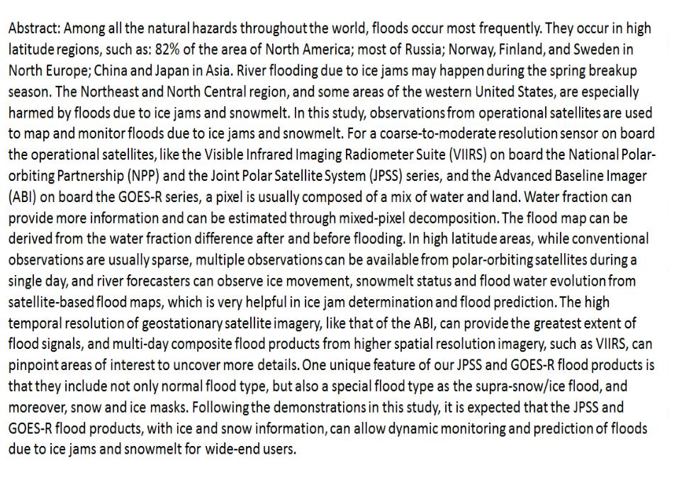
Abstract
:
1. Introduction
2. Data and Methods
2.1. Study Sites
2.2. Data Used
- Calibrated VIIRS level 1b data at imagery channel 1 (red: 600–680 nm), channel 2 (near-infrared: 850–880 nm), channel 3 (shortwave infrared: 1610 nm), and thermal infrared channel 5 (1050–1240 nm) with 375-m spatial resolution.
- The calibrated level 1b GOES-16 ABI near real-time data
- GOES-R and VIIRS geolocation data, including longitude, latitude, solar zenith angles, solar azimuth angles, sensor zenith angles and sensor azimuth angles.
- S-NPP/VIIRS cloud mask Intermediate Product at 750-m resolution
- M-band terrain-corrected geolocation data (GMTCO).
- The National Land Cover Database 2006 (NLCD) of the United States Geological Survey (USGS) [27].
- Linear hydrographic feature data, including major rivers, streams and canals, and area hydrographic feature data, including major lakes and reservoirs.
2.3. Methods
2.3.1. Flooding Water Detection
2.3.2. Cloud Shadow Removal
2.3.3. Terrain Shadow Removal
2.3.4. Flooding Water Fraction Derivation
3. Results
4. Discussion
5. Conclusions
Author Contributions
Funding
Acknowledgments
Conflicts of Interest
References
- Sun, Z.; Sui, J. Calculation of water level in a river reach with frazil ice jam. In Proceedings of the 10th IAHR Symposium on Ice Problems, Espoo, Finland, 20–23 August 1990; Volume II, pp. 756–765. [Google Scholar]
- Tropeano, D.; Turconi, L. Geomorphic classification of alpine catchments for debris-flow hazard reduction. In Proceedings of the International Conference on Debris-Flow Hazards Mitigation: Mechanics, Prediction and Assessment, Davos, Switzerland, 10–12 September 2003; Millpress Science Pub: Rotterdam, Switzerland, 2003; Volume 2, pp. 1221–1232. [Google Scholar]
- Goldberg, M.D.; Cikanec, H.A.; Zhou, L.; Price, J. The join polar satellite system. In Comprehensive Remote Sensing; Liang, S., Ed.; Elsevier: New York, NY, USA, 2017; p. 108. ISBN 9780128032206. [Google Scholar]
- Wang, C. Numerical Modelling of Ice Floods in the Ning-Meng Reach of the Yellow River Basin. Dissertation, 2017. Available online: https://www.un-ihe.org/sites/default/files/2017_unesco-ihe_phd_thesis_wang_i.pdf (accessed on 4 June 2020).
- Marchil, L.; Chiarle, M.; Mortara, G. Climate changes and debris flows in periglacial areas in the Italian Alps. In From Headwaters to the Ocean: Hydrological Changes and Watershed Management; Taniguchi, M., Burnett, W.C., Fukushima, Y., Haigh, M., Umezawa, Y., Eds.; Taylor and Francis: London, UK, 2009; pp. 111–113. [Google Scholar]
- Nigrelli, G.; Fratianni, S.; Zampollo, A.; Turconi, L.; Chiarle, M. The altitudinal temperature lapse rates applied to high elevation rockfalls studies in the Western European Alps. Theor. Appl. Climatol. 2018, 131, 1479–1491. [Google Scholar] [CrossRef]
- Turconi, L.; De, S.K.; Tropeano, D.; Savio, G. Slope failure and related processes in the Mt. Rocciamelone area (Cenischia valley, Western Italian). Geomorphology 2010, 114, 115–128. [Google Scholar] [CrossRef]
- Thériault, I.; Saucet, J.-P.; Taha, W. Validation of the mike-ice model simulating river flows in presence of ice and forecast of changes to the ice regime of the romaine river due to hydroelectric project. In Proceedings of the 20th IAHR International Symposium on Ice, Lahti, Finland, 14–17 June 2010. [Google Scholar]
- Chen, F.; Shen, H.T.; Jayasundara, N. A one-dimensional comprehensive river ice model. In Proceedings of the 18th International Association of Hydraulic Research Symposium on ice, Sapporo, Japan, 28 August–1 September 2006. [Google Scholar]
- Blackburn, J.; She, Y. A comprehensive public-domain river ice process model and its application to a complex natural river. Cold Reg. Sci. Technol. 2019, 163, 44–58. [Google Scholar] [CrossRef]
- Lindenschmidt, K.-E. RIVICE—A non-proprietary, open-source, one-dimensional river-ice and water-quality model. Water 2017, 9, 314. [Google Scholar] [CrossRef]
- Yu, K.X.; Zhang, X.; Li, L.; Zhan, B.; Qin, Y.; Su, Q. Probability prediction of peak breakup water level through vine copulas. Hydrol. Process. 2019, 33, 962–977. [Google Scholar] [CrossRef]
- Sheng, Y.; Gong, P.; Xiao, Q. Quantitative dynamic flood monitoring with NOAA AVHRR. Int. J. Remote Sens. 2001, 22, 1709–1724. [Google Scholar] [CrossRef]
- Sun, D.; Yu, Y.; Goldberg, M. Deriving water fraction and flood maps from MODIS images using a decision tree approach. IEEE J. Sel. Top. Appl. Earth Observ. Remote Sens. 2011, 4, 814–825. [Google Scholar] [CrossRef]
- Sun, D.; Yu, Y.; Zhang, R.; Li, S.; Goldberg, M. Towards operational automatic flood detection using EOS/MODIS data. Photogramm. Eng. Rem. Sens. 2012, 78, 637–646. [Google Scholar] [CrossRef]
- Li, S.; Sun, D.; Yu, Y.; Csiszar, I.; Stefanidis, A.; Goldberg, M. A New Shortwave Infrared (SWIR) Method for Quantitative Water Fraction Derivation and Evaluation with EOS/MODIS and Landsat/TM data. IEEE Trans. Geosci. Remote Sens. 2012, 51, 1852–1862. [Google Scholar] [CrossRef]
- Bates, P.D.; Wilson, M.D.; Horritt, M.S.; Mason, D.C.; Holden, N.; Currie, A. Reach scale flood plain inundation dynamics observed using airborne synthetic aperture radar imagery: Data analysis and modeling. J. Hydrol. 2006, 328, 306–318. [Google Scholar] [CrossRef]
- Sippel, S.J.; Hamilton, S.K.; Melack, J.M.; Choudhury, B.J. Determination of inundation area in the Amazon river floodplain using the SMMR 37 GHz polarization difference. Remote Sens. Environ. 1994, 48, 70–76. [Google Scholar] [CrossRef]
- Jin, Y.Q. Flooding index and its regional threshold value for monitoring floods in China from SSM/I data. Int. J. Remote Sens. 1999, 20, 1025–1030. [Google Scholar] [CrossRef]
- Tanaka, M.; Sugimura, T.; Tanaka, S.; Tamai, N. Flood drought cycle of Tonle Sap and Mekong Delta area observed by DMSP-SSM/I. Int. J. Remote Sens. 2003, 24, 1487–1504. [Google Scholar] [CrossRef]
- Temimi, M.; Leconte, R.; Brissette, F.; Chaouch, N. Flood and soil wetness monitoring over the Mackenzie River Basin using AMSR-E 37 GHz brightness temperature. J. Hydrol. 2007, 333, 317–328. [Google Scholar] [CrossRef]
- Zheng, W.; Liu, C.; Wang, Z.X.; Xin, Z.B. Flood and waterlogging monitoring over Huaihe River Basin by AMSR-E data analysis. Chin. Geogr. Sci. 2008, 18, 262–267. [Google Scholar] [CrossRef] [Green Version]
- Beaton, A.; Whaley, R.; Corston, K.; Kenny, F. Identifying historic river ice breakup timing using MODIS and Google earth engine in support of operational flood monitoring in northern Ontario. Remote Sens. Environ. 2019, 224, 352–364. [Google Scholar] [CrossRef]
- Lindenschmidt, K.E.; Li, Z. Radar scatter decomposition to differentiate between running ice accumulations and intact ice covers along rivers. Remote Sens. 2019, 11, 307. [Google Scholar] [CrossRef] [Green Version]
- Lindenschmidt, K.E.; Rokaya, P.; Das, A.; Li, Z.; Richard, D. A novel stochastic modelling approach for operational real-time ice-jam flood forecasting. J. Hydrol. 2019, 575, 381–394. [Google Scholar] [CrossRef]
- JPSS Proving Ground Portfolio, 2018–2021. Available online: https://www.jpss.noaa.gov/assets/pdfs/2018%20JPSS%20PGRR%20Portfolio.pdf (accessed on 4 June 2020).
- Xian, G.; Homer, C.; Dewitz, J.; Fry, J.; Hossain, N.; Wickham, J. The change of impervious surface area between 2001 and 2006 in the conterminous United States. Photogramm. Eng. Remote Sens. 2011, 77, 758–762. [Google Scholar]
- Rabus, B.; Eineder, M.; Roth, A.; Bamler, R. The shuttle radar topography mission—A new class of digital elevation models acquired by spaceborne radar. Photogramm. Remote Sens. 2003, 57, 241–262. [Google Scholar] [CrossRef]
- Carroll, M.; Townshend, J.; DiMiceli, C.; Noojipady, P.; Sohlberg, R. A New Global Raster Water Mask at 250 Meter Resolution. Int. J. Dig. Earth 2009, 2, 291–308. [Google Scholar] [CrossRef]
- Liang, Y.-L.; Colgan, W.; Lv, Q.; Steffen, K.; Abdalati, W.; Stroeve, J.; Gallaherb, D.; Bayou, N. A decadal investigation of supraglacial lakes in West Greenland using a fully automatic detection and tracking algorithm. Remote Sens. Environ. 2012, 123, 127–138. [Google Scholar] [CrossRef] [Green Version]
- Johansson, A.M.; Brown, I.A. Adaptive classification of supraglacial lakes on the West Greenland ice sheet. IEEE J. Sel. Top. Appl. Earth Obs. Remote Sens. 2013, 6, 1998–2007. [Google Scholar] [CrossRef]
- Lesson, A.; Leeson, A.; Shepherd, A.; Sundal, A.V.; Johansson, A.M.; Selmes, N.; Briggs, K.; Hogg, A.E.; Fettweis, X. A comparison of supraglacial lake observations derived from MODIS imagery at the western margin of the Greenland ice sheet. J. Glaciol. 2013, 59, 1179–1188. [Google Scholar] [CrossRef] [Green Version]
- Li, S.; Sun, D.; Goldberg, M.D.; Sjoberg, B.; Santek, D.; Hoffman, J.P.; DeWeese, M.; Restrepo, P.; Lindsey, S.; Holloway, E. Automatic near real-time flood detection using Suomi-NPP/VIIRS data. Remote Sens. Environ. 2017, 204, 672–689. [Google Scholar] [CrossRef]
- Li, S.; Sun, D.; Yu, Y. Automatic cloud-shadow removal from flood/standing water maps using MSG/SEVIRI imagery. Int. J. Remote Sens. 2013, 34, 5487–5502. [Google Scholar] [CrossRef]
- Li, S.; Sun, D.; Goldberg, M.D.; Sjoberg, W. Object-based automatic terrain shadow removal from SNPP/VIIRS flood maps. Int. J. Remote Sens. 2015, 36, 5504–5522. [Google Scholar] [CrossRef]
- Shepard, M.K.; Campbell, B.A.; Bulmer, M.H.; Farr, T.G.; Gaddis, L.R.; Plaut, J.J. The roughness of natural terrain: A planetary and remote sensing perspective. J. Geophys. Res. 2001, 106, 32777–32795. [Google Scholar] [CrossRef]
- Goldberg, M.; Li, S.; Goodman, S.; Lindsey, D.; Sjoberg, D.; Sun, D. Contributions of Operational Satellites in Monitoring the Catastrophic Floodwaters Due to Hurricane Harvey. Remote Sens. 2018, 10, 1256. [Google Scholar] [CrossRef] [Green Version]
- The Sentinel-Hub EO Browser. Available online: https://apps.sentinel-hub.com/eo-browser (accessed on 4 June 2020).
- VIIRS Flood Products in Near Real Time. Available online: http://wms.ssec.wisc.edu/s/A8LT (accessed on 4 June 2020).
- JPSS Proving Ground Global Flood Products Archive. Available online: https://jpssflood.gmu.edu/ (accessed on 4 June 2020).
- Rokaya, P.; Morales-Marin, L.; Lindenschmidt, K.E. A physically-based modelling framework for operational forecasting of river ice breakup. Adv. Water Resour. 2020, 139, 103554. [Google Scholar] [CrossRef]
- Morales-Marín, L.A.; Sanyal, P.R.; Kadowaki, H.; Li, Z.; Rokaya, P.; Lindenschmidt, K.E. A hydrological and water temperature modelling framework to simulate the timing of river freeze-up and ice-cover breakup in large-scale catchments. Environ. Model. Softw. 2019, 114, 49–63. [Google Scholar] [CrossRef]


© 2020 by the authors. Licensee MDPI, Basel, Switzerland. This article is an open access article distributed under the terms and conditions of the Creative Commons Attribution (CC BY) license (http://creativecommons.org/licenses/by/4.0/).
Share and Cite
Goldberg, M.D.; Li, S.; Lindsey, D.T.; Sjoberg, W.; Zhou, L.; Sun, D. Mapping, Monitoring, and Prediction of Floods Due to Ice Jam and Snowmelt with Operational Weather Satellites. Remote Sens. 2020, 12, 1865. https://0-doi-org.brum.beds.ac.uk/10.3390/rs12111865
Goldberg MD, Li S, Lindsey DT, Sjoberg W, Zhou L, Sun D. Mapping, Monitoring, and Prediction of Floods Due to Ice Jam and Snowmelt with Operational Weather Satellites. Remote Sensing. 2020; 12(11):1865. https://0-doi-org.brum.beds.ac.uk/10.3390/rs12111865
Chicago/Turabian StyleGoldberg, Mitchell D., Sanmei Li, Daniel T. Lindsey, William Sjoberg, Lihang Zhou, and Donglian Sun. 2020. "Mapping, Monitoring, and Prediction of Floods Due to Ice Jam and Snowmelt with Operational Weather Satellites" Remote Sensing 12, no. 11: 1865. https://0-doi-org.brum.beds.ac.uk/10.3390/rs12111865