Evaluation of Two Global Land Surface Albedo Datasets Distributed by the Copernicus Climate Change Service and the EUMETSAT LSA-SAF

Abstract

The present paper is devoted to the quality assessment of two global land surface albedo products developed by Meteo France in the frame of the Copernicus Climate Change Service (C3S) and the LSA-SAF (Satellite Application Facility on Land Surface Analysis), herein called, respectively, VGT (VeGeTation) (the C3Sv1 dataset, derived from VGT sensors onboard Satellites for the Observation of the Earth, also called SPOT) and ETAL (European polar system Ten-day surface ALbedo, derived from Advanced Very High Resolution Radiometers (AVHRR) onboard METeorological OPerational (METOP) satellites). The evaluation study inter-compared these products with measurements at 33 ground stations and two independent operational products, MTAL-R/NRT (Meteosat second generation Ten-day ALbedo Reprocessed/Near Real-Time) and MODIS (MODerate resolution Imaging Spectroradiometer), over two distinct four-year periods. In accordance with the prescription from the Land Product Validation group of the joint Committee on Earth Observation Satellites (LPV/CEOS), the evaluation was addressed per land cover; furthermore, two albedo regimes were considered throughout the evaluation to distinguish between high (over 0.15) and low (below 0.15) surface albedo behaviors. First, we show that both VGT and ETAL products agree well with the measurements and the other satellite products at the ground stations. Second, when inter-compared with MODIS, the results are noteworthy for ETAL as opposed to VGT, with 11 out of 13 land cover types passing the Global Climate Observing System (GCOS) requirements for more than 80% of the sites for albedo values less than 0.15 (compared with none for VGT) and 10 out of 14 land cover types passing the GCOS requirements for more than 50% of the sites for albedo values greater than 0.15 (compared with 5 for VGT). Finally, a pixel-by-pixel analysis reveals that VGT overestimates the surface albedo as compared with MODIS by about 0.02 in absolute value for albedo values less than 0.15 and by about 22% in relative value for albedo values greater than 0.15. The root-mean-square-deviation (RMSD) in absolute value is about 0.015 for albedo values less than 0.15 and 51.5% in relative value for albedo values greater than 0.15. In contrast, the bias for ETAL when compared with MODIS remains very small. Over the four-year period, ETAL overestimates the surface albedo as compared with MODIS by 0.001 in absolute value for the regime of surface albedo less than 0.15 and by about 5.8% in relative value for albedo values greater than 0.15. The RMSD in absolute value is about 0.014 for albedo values less than 0.15 and 19.4% in relative value for albedo values greater than 0.15. Assuming that the MODIS product is a good reference, a relative bias of around 6% can be judged satisfactory for ETAL surface albedo. The lower performance of the VGT (C3Sv1) product is currently the subject of investigation. Work is ongoing to upgrade it further towards the final C3S product.

1. Introduction

Climate monitoring is of paramount importance in the context of climate change [1]. Long-term monitoring of Essential Climate Variables (ECV) through observatories from Earth Observation (EO) instruments onboard geostationary and polar-orbiting satellite systems is a key infrastructure addressing this challenge [2,3].

Land surface albedo is one such ECV and it is defined as the ratio of the upward and downward radiation at the Earth’s surface [4,5]. A decrease in surface albedo (which is observed, for example, when ice is melting) can induce prejudicial consequences to the Earth’s energy balance [6,7]. Admittedly, climate model surface albedos and other related variables will be improved with satellite measurements (e.g., [8]), but the high sensitivity of the Earth’s climate in terms of surface albedo calls for highly accurate surface albedo products [9]. Other benefits of accurate surface albedo products include weather forecasting [10] and land cover monitoring; more particularly, land surface albedo can significantly contribute to the analysis of desertification processes or the identification of trends in vegetation variability [3].

In the frame of the Copernicus Climate Change Service (C3S, https://climate.copernicus.eu), the C3Sv1 VeGeTation (VGT) surface albedo product has been recently derived from data collected by the VGT1 instrument onboard the SPOT-4 (Satellite for the Observation of the Earth) satellite during the period 1998–2003 and the VGT2 sensor onboard SPOT-5 during the period 2003–2014. This dataset is currently available from the Copernicus Climate Data Store (CDS) at https://cds.climate.copernicus.eu/cdsapp#!/dataset/satellite-albedo?tab=overview. In 2019, the Copernicus/C3S program produced a continuous and homogeneous time series for a 40-year period, from 1981 until now, by merging observations from VGT and Advanced Very High Resolution Radiometers (AVHRR) sensors.

The European polar system Ten-day ALbedo (ETAL, https://landsaf.ipma.pt/en/products/albedo/etal/) surface albedo product derived from AVHRR sensors onboard the European polar satellite series (METeorological OPerational, METOP A/B/C) is another global product that has been made available recently via the European Organization for the Exploitation of Meteorological Satellites (EUMETSAT) Satellite Application Facility (SAF) on Land Surface Analysis (LSA) [11].

Both VGT and ETAL products supplement other surface albedo satellite products [12] derived, in the last two decades, from different spaceborne instruments, including Advanced Very High Resolution Radiometers (AVHRR) [13,14], POLarization and Directionality of the Earth’s Reflectances (POLDER) [15], MODerate resolution Imaging Spectroradiometers (MODIS) [16], Meteosat Visible and InfraRed Imagers (MVIRI) [17], Airborne Visible-InfraRed Imaging Spectrometer (AVIRIS) [18], VEGETATION (VGT) [19,20], PROBA-VEGETATION (PROBA-V) [20], Visible Infrared Imaging Radiometer Suite (VIIRS) [21], Geostationary Operational Environmental Satellites (GOES-R) [22] and Spinning Enhanced Visible and Infrared Imagers (SEVIRI) [23]. Several initiatives, such as GlobAlbedo [24,25] or Global LAnd Surface Satellites (GLASS) [26], have provided long-term albedo products from these satellite data.

Although MODIS surface albedo products are widely used, the MODIS sensors onboard the Terra and Aqua satellites have been operating for a period of time that far exceeds their expected life duration (orbiting since 1999 and 2002, respectively). Hence, surface albedo products already available from other satellite missions, such as the National Oceanic and Atmospheric Administration (NOAA) VIIRS [21], SPOT/VGT [20,27] and METOP/AVHRR for the ETAL product [28], could offer service continuity to the scientific community.

A general framework for the Evaluation and Quality Control (EQC) of climate data products derived from satellite observations aimed to be released by the Copernicus CDS has been proposed [29]. The validation and the quality assessment of the products by independent means are pinpointed. To this end, two different approaches are identified: direct and indirect assessments. On the one hand, direct point-to-pixel comparisons shall be performed with respect to ground measurements from tower-based instruments, in the case of surface albedo. Here, the spatial representativeness of the site is critical, as explained by Roman et al. [30,31]. On the other hand, an indirect validation based on exhaustive inter-comparisons with heritage satellite products needs to be considered. The latter can reveal spatial disagreements between albedo products over large areas and for a wide range of cover types. For the case of surface albedo, the Land Product Validation group of the joint Committee on Earth Observation Satellites (LPV/CEOS) issued recommendations on how to address both direct and indirect validations [32], based on a number of metrics that can be analytically calculated.

This paper aims to evaluate the two new VGT and ETAL surface albedo products developed by Meteo France in the Framework of Copernicus/C3S and LSA-SAF programs, respectively, following those prescriptions. Because the products were not available for the same period of time, two distinct four-year periods for VGT (2009–2012) and ETAL (2015–2018) were considered. A time extent of four years is deemed long enough for the analysis. The shortwave directional-hemispherical (SW-DH) surface albedo was used for the evaluation. This approach follows from past evaluation studies [33,34] of surface albedo products retrieved from MODIS [16] and the Multiangle Imaging SpectroRadiometer (MISR) [35] sensors onboard polar satellites and other products retrieved from sensors onboard geostationary satellites [23,36,37,38,39].

In earlier attempts to validate satellite-derived surface albedo products [23,36], root-mean-square deviation (RMSD) values under 0.04 were found when inter-comparing Meteosat Second Generation (MSG) surface albedo data, including products acquired in the presence of snow, with other satellite products, such as MODIS and SPOT-VGT. Furthermore, in a recent study [40], RMSD values under 0.04 were also found for MODIS MCD43A3, Global Land Surface Satellite (GLASS) and the forthcoming Multi-source Data Synergized Quantitative Remote Sensing Production system (MuSyQ) albedos using ground observations and Huan Jing (HJ) data.

This paper is organised as follows. Section 2 presents the two datasets under test, the evaluation protocol, the applicable requirements and the validation datasets used. In Section 3, results from three different analyses both direct and indirect are provided and discussed. Finally, conclusions are drawn in Section 4.

2. Data and Protocol

2.1. Satellite Data

2.1.1. Surface Albedo Characteristics

Because the surface albedo retrieved from spacecraft uses observations over few spectral bands (in the visible and near-infrared range), conversions are needed to transform spectral albedo values into broadband albedos [41].

Admittedly, the shortwave broadband albedo ([0.3–4.0 $\mathsf{\mu }$m]) that encompasses all spectral bands of the solar spectrum (the visible and near-infrared bands) is the preferred candidate for evaluation studies [3].

Alongside the spectral aspect, two surface albedo concepts have been proposed that differ depending on whether the illumination is considered a point source or a full half-hemisphere while the view is assumed to be a full half-hemisphere [42,43]. Both cases correspond to extreme situations in which a sunny, cloud-free sky or a full cloudy sky would occur. Over the past two decades, there has been considerable progress in the inversion of satellite measurements into those values and many more [41,43,44]. The first case is referred to as directional-hemispherical (DH), and the second case is referred to as bi-hemispherical (BH).

For the sake of our analyses, the DH surface albedo is evaluated. In reality, the true surface albedo is a mix of both albedo types and is usually referred to as blue surface albedo. The shortwave directional-hemispherical (SW-DH) surface albedo is evaluated throughout this paper. Without further indication, all surface albedo quantities refer to SW-DH quantities.

2.1.2. VGT and ETAL Surface Albedo

The surface albedo retrievals are generated by VITO (the Flemish institute for technological research) for VGT and by IPMA (Portuguese Institute of the Sea and the Atmosphere) for ETAL. At the input of the operational chains, one finds radiance measurements acquired in four (respectively, three) channels of the VGT (respectively, AVHRR) sensor for VGT (respectively, ETAL), whose spectral characteristics are recalled in

Table 1. Spectral characteristics of VGT, ETAL, MTAL and MODIS.

	VGT			ETAL			MTAL			MODIS
	Name	Center (nm)	Width (nm)	Name	Center (nm)	Width (nm)	Name	Center (nm)	Width (nm)	Name	Center (nm)	Width (nm)
Blue	B0	458	37	n.a.	n.a.	n.a.	n.a.	n.a.	n.a.	Band3	469	20
Red	B2	653	74	Ch.1	630	100	VIS0.6	635	150	Band1	645	50
NIR	B3	838	109	Ch.2	865	275	VIS0.8	810	140	Band2	858.5	35
SWIR	MIR	1635	101	Ch.3a	1610	60	NIR1.6	1600	280	Band6	1640	24

(http://www.spot-vegetation.com/pages/SPOT_VGT_PUM_v1.0.pdf for VGT and http://www.eumetsat.int/website/wcm/idc/idcplg?IdcService=GET_FILE&dDocName=PDF_AVHRR_L1B_PRODUCT_GUIDE&RevisionSelectionMethod=LatestReleased&Rendition=Web for ETAL, last access: May 2020). The retrieval methods follow the same methodology with slight differences. First, the top-of-atmosphere (TOA) data from the different spectral channels are processed in order to obtain cloud-free top-of-canopy (TOC) reflectances. While this atmospheric correction step uses MERRA-2 (the Modern-Era Retrospective analysis for Research and Applications, Version 2) reanalyses for VGT, one relies on a climatology (on the basis of the Copernicus Atmosphere Monitoring Service, CAMS) for the aerosol contribution in ETAL. Then, the spectral TOC reflectances acquired under different solar-viewing configurations during the synthesis period are normalised by inverting a linear kernel-driven model. Both products rely on the Ross Thick kernel for volumetric scattering and Li Sparse-Reciprocal kernel for geometrical scattering (RTLSR) [44]. Either products have a 20-day synthesis period with the maximum weight on the last observation of the period. The spectral albedos are then computed by means of angular integrations of the kernel functions with the retrieved parameters for each pixel. Finally, the broadband surface albedo is defined as a linear combination of the spectral albedo values in the available spectral channels. The narrow-to-broadband conversion coefficients are applied both for the DH and for the BH albedos. The algorithm includes uncertainty estimation at different levels of the processing starting from the TOA reflectance and a Kalman filter approach is taken in order to propagate those uncertainties so as to avoid gaps in the product due to persistent cloudy conditions. More details about the data generation can be found within the documentation [27] for VGT and in here [23,45] for ETAL.

The characteristics in terms of spectral properties, coverage, spatial resolution and frequency of production are similar for both products. They are summarized in

Table 2. SPOT-VGT Copernicus Climate Change Service (VGT-C3S)-based Ten-day and Land Surface Analysis Satellite Application Facility (LSA-SAF) European Polar System (EPS) Metop-based Ten-day Albedo (ETAL) surface albedo product characteristics.

Product Variable	Product Key	Product ID	Product Name	Coverage	Spatial Resolution	Composite Period	Frequency of Production
Total shortwave directional-hemispherical broadband albedo [0.3–4.0 $\mathsf{\mu }$m]	SW-DH	SA	VGT	Full globe	∼1 km × 1 km	20 days	10 days (10th, 20th and last day of each month)
Total shortwave directional-hemispherical broadband albedo [0.3–4.0 $\mathsf{\mu }$m]	SW-DH	LSA-103	ETAL	Full globe	∼1 km × 1 km	20 days	10 days (5th, 15th and 25th of each month)

. Because the products were not available for the same period of time (1998–2014 for VGT and 2015–2018 for ETAL), two different time windows were considered throughout our analysis, as discussed in Section 2.3.

2.1.3. MODIS Surface Albedo

MODIS land surface albedo data are widely used by the satellite and modeling communities for evaluating other satellite albedo data (e.g., [46]) and also for refining models. Data from both Terra and Aqua satellites are used in the generation of this product. For the current evaluation exercise, MODIS collection 6 products that achieved CEOS LPV stage 3 validation are used. Besides, published research indicates that the accuracy of the MODIS shortwave broadband albedo meets the GCOS [3] accuracy requirements (≤5%) for both snow-free and snow-covered surfaces [47,48].

Land surface albedo (Directional-Hemispherical product ref. MCD43D51) and associated quality flags (ref. MCD43D31) are provided as full-globe datasets projected on an equirectangular grid (approximately 1 km of spatial resolution). These two products are made available on a daily basis and are computed by integrating a 16-day sliding window. Unlike VGT and ETAL, MODIS uses its own daily aerosol product [49], but like the other two products it applies the same parametric Bidirectional Reflectance Distribution Function (BRDF) model, viz. the RTLSR [44]. Its spectral channels relevant for the calculation of the surface albedo are recalled in Table 1 (https://modis.gsfc.nasa.gov/about/specifications.php, last access: May 2020). MODIS broadband surface albedo spectral extent is slightly greater ([0.3–5.0 $\mathsf{\mu }$m] for the shortwave) than that of ETAL and VGT (refer to Table 2). Nonetheless, the solar energy between 4 and 5 $\mathsf{\mu }$ m is not significant compared with the rest of the solar spectral domain; hence, the inter-comparison remains relevant. More information with respect to the surface albedo retrieval algorithm implemented in MODIS is found here: https://modis.gsfc.nasa.gov/data/atbd/atbd_mod09.pdf. Aspects concerning the preprocessing and re-projection of MODIS data are discussed in Section 2.5.

2.1.4. MTAL (R/NRT) Surface Albedo Products

MTAL (Meteosat second generation Ten-day ALbedo) is the geostationnary counterpart of ETAL and another LSA-SAF albedo product. It is derived from data acquired by the SEVIRI sensor onboard MSG satellites, whose channels have similar spectral properties as VGT and ETAL (see Table 1) [50]. The spatial coverage of the MSG disk includes Europe, Africa and South America. It exists in the form of a reprocessed (MTAL-R) or near real-time (MTAL-NRT) product. The retrieval methodology is again similar to that of ETAL and VGT since all rely on the same heritage algorithm. The difference between the climate data record CDR (MTAL-R) and NRT albedo products is the different input data used for the atmospheric correction. For the CDR MTAL-R product, atmospheric reanalyses from the European Center for Medium-Range Weather Forecasts (ECMWF) are used instead of forecasted fields. Other input data are the same as those for the MSG daily albedo product, as described in Geiger [41]. The periods of availability of both products differ, as presented in Section 2.3. In fact, the evaluation of VGT includes MTAL-R, while the evaluation of ETAL includes MTAL-R (for 2015) and MTAL-NRT (available for the three-year period from 2016 to 2018). More information concerning MTAL R/NRT is available in [45] and an exhaustive validation exercise over MTAL-R is accessible in [23]. It was shown that MTAL-R meets the users requirements (≤5%).

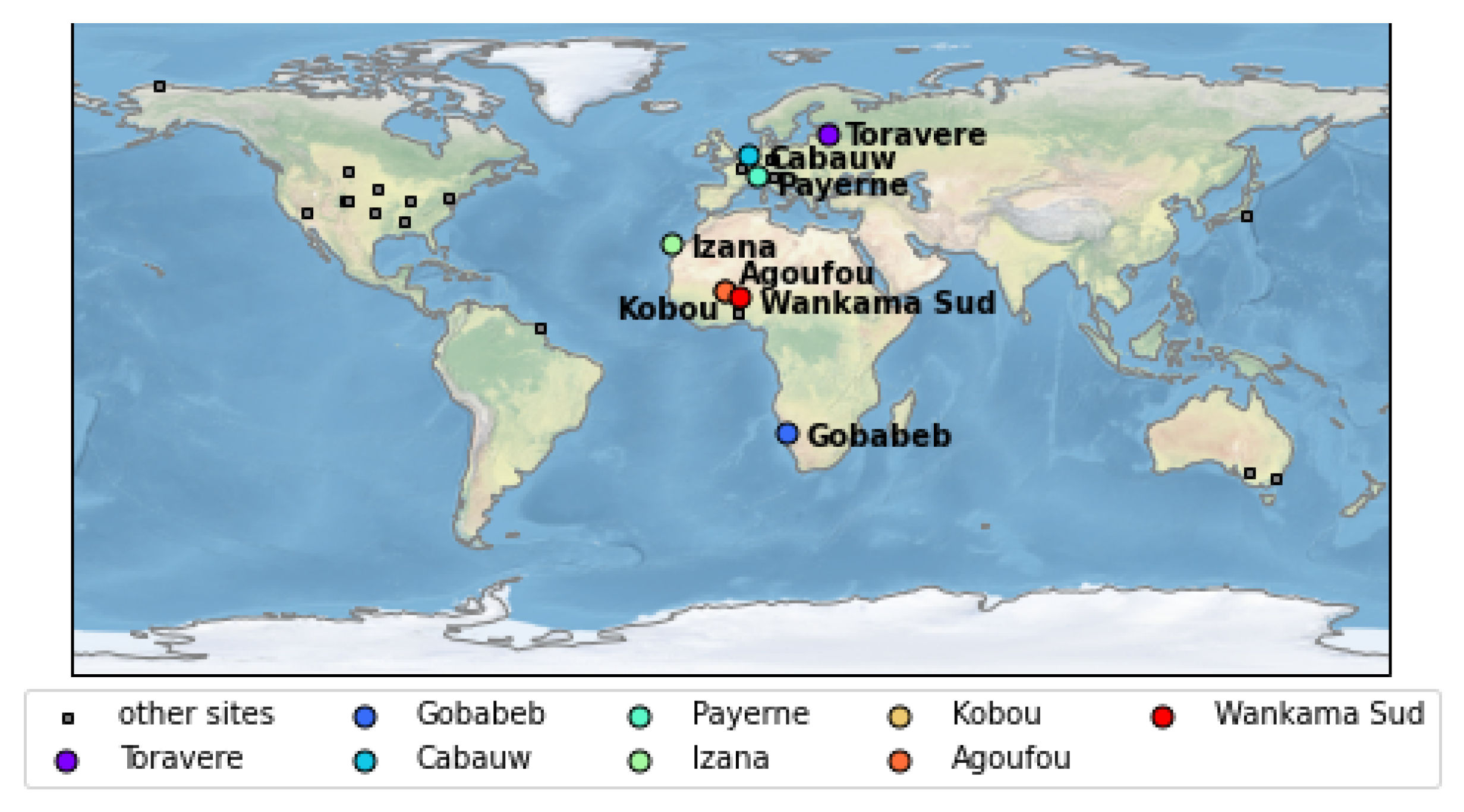
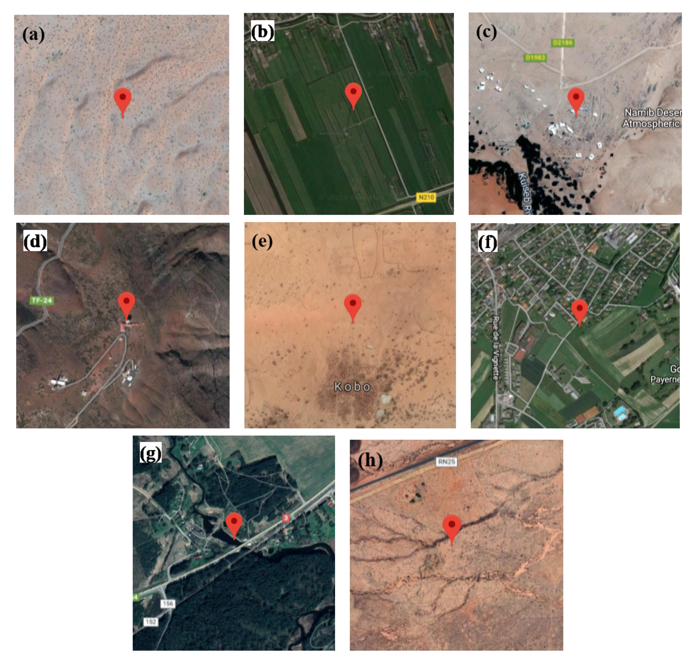
2.2. Ground Observations

Thirty-three ground stations were considered for the direct evaluation of the satellite-derived albedos (

Table 3. List of all ground stations used for the accuracy analyses.

Station	Lon (°E)	Lat (°N)	Country	Data Source	Availability (Start)	Availability (End)	Land Classification (IGBP)	In MSG Disk?	Available on VGT (2009–2012); ETAL (2015–2018)
Wankama flux sud	26,298	13,644	Niger	AMMA CATCH	01/2005	2014	Grasslands	Y	VGT (4 years)
Bamba	−14,018	17,099	Mali	AMMA CATCH	01/2005	2010	Barren or sparsely vegetated	Y	VGT (2 years)
Agoufou	−14,791	153,445	Mali	AMMA CATCH	01/2005	2011	Grasslands	Y	VGT (3 years)
Kobou	−15,021	147,284	Mali	AMMA CATCH	01/2008	2011	Grasslands	Y	VGT (3 years)
Wankama flux nord	26,337	136,476	Niger	AMMA CATCH	01/2005	2014	Grasslands	Y	VGT (4 years)
Bira flux	17,167	98,267	Benin	AMMA CATCH	01/2005	31/12/2015	Savannas	Y	VGT (4 years) + ETAL (1 year)
Djougou	16,615	9692	Benin	AMMA CATCH	01/2011	05/06/2016	Savannas	Y	VGT (2 years) + ETAL (1.5 years)
Nalohou flux	16,046	97,448	Benin	AMMA CATCH	01/2005	31/12/2015	Savannas	Y	VGT (4 years) + ETAL (1 year)
Gobabeb	15,042	−235,614	Namibia	BSRN	15/05/2012	current	Barren or sparsely vegetated	Y	VGT (0.5 year) + ETAL (4 years)
Cabauw	49,267	519,711	The Netherlands	BSRN	01/12/2005	current	Cropland and natural vegetation mosaic	Y	VGT (4 years) + ETAL (4 years)
Payerne	6944	46,815	Switzerland	BSRN	01/09/1992	2014	Cropland and natural vegetation mosaic	Y	VGT (4 years)
Tateno	1,401,258	360,581	Japan	BSRN	01/02/1996	current	Croplands	N	VGT (4 years) + ETAL (4 years)
Toravere	26,462	58,254	Estonia	BSRN	01/01/1999	current	Mixed forest	Y	VGT (4 years) + ETAL (4 years)
Izana	−164,993	283,093	Canarias Spain	BSRN	01/12/2016	current	Open shrublands	Y	ETAL (2 years)
GoodwinCreek	−898,729	342,547	USA	GBOV	03/01/2013	24/12/2016	Deciduous broadleaf forest	N	ETAL (2 years)
Hainich	10,453	510,792	Germany	GBOV	03/01/2012	24/12/2015	Mixed forest	Y	VGT (1 year) + ETAL (1 year)
Bondville	−883,731	400,519	USA	GBOV	03/01/2013	24/12/2016	Croplands	N	ETAL (2 years)
Gebesee	109,143	511,001	Germany	GBOV	03/01/2012	24/12/2015	Croplands	Y	VGT (1 year) + ETAL (1 year)
Grignon	195,191	488,442	France	GBOV	03/01/2012	24/12/2015	Croplands	Y	VGT (1 year) + ETAL (1 year)
SiouxFallsSurfRad	−966,233	43,734	USA	GBOV	03/01/2013	24/12/2016	Croplands	N	ETAL (2 years)
SouthernGreatPlains	−97,485	36,605	USA	GBOV	03/01/2012	24/12/2016	Croplands	N	VGT (1 year) + ETAL (2 years)
RockSprings	−779,308	407,201	USA	GBOV	03/01/2013	24/12/2016	Deciduous broadleaf forest	N	ETAL (2 years)
Guyaflux	−529,249	52,788	French Guyana	GBOV	03/01/2012	24/12/2015	Evergreen broadleaf forest	N	VGT (1 year) + ETAL (1 year)
Tumbarumba	148,152	−356,566	Australia	GBOV	03/01/2013	24/12/2016	Evergreen broadleaf forest	N	ETAL (2 years)
NiwotRidgeForest	−105,546	400,329	USA	GBOV	03/01/2013	24/12/2016	Evergreen needleleaf forest	N	ETAL (2years)
Barrow	−156,611	71,323	USA	GBOV	03/03/2013	13/10/2016	Snow and ice	N	ETAL (2 years)
Boulder	−105,007	4005	USA	GBOV	03/01/2012	24/12/2015	Cropland and natural vegetation mosaic	N	VGT (1 year) + ETAL (1year)
FortPeck	−105,102	483,078	USA	GBOV	03/01/2013	24/12/2016	Grasslands	N	ETAL (2years)
Renon	114,337	465,869	Italy	GBOV	03/01/2012	24/12/2015	Evergreen needleleaf forest	Y	VGT (1 year) + ETAL (1 year)
TableMountain	−105,237	40,125	USA	GBOV	03/01/2013	24/12/2016	Barren or sparsely vegetated	N	ETAL (2years)
Brasschaat	45,206	513,092	Belgium	GBOV	03/01/2013	24/12/2016	Mixed forest	Y	ETAL (2 years)
Calperum	140,588	−340,027	Australia	GBOV	03/01/2013	24/12/2016	Closed shrublands	N	ETAL (2 years)
DesertRock	−116,019	366,237	USA	GBOV	03/01/2013	24/12/2016	Open shrublands	N	ETAL (2 years)

). Their positions are displayed in Figure 1.

Following the prescription from the Land Product Validation (LPV) group of the joint CEOS [32], these ground stations were chosen because they cover a large range of land covers (12 of the 17 International Geosphere-Biosphere Programme IGBP classes). Even though the representativeness of each individual station in agreement to Roman criteria [30,31] could not be assessed, they are deemed reasonable for the level of qualitative analysis at stake in this work, similar to what was done by Carrer et al. [23]. More details upon representativeness aspects of the measurement sites can be gathered from http://savs.eumetsat.int/ [51].

The generation of the ground albedo equivalent values is described as follows:

• Baseline Surface Radiation Network (BSRN, https://bsrn.awi.de/) [52,53]: Radiation data are acquired every 1–3 min. Measurements acquired with a solar zenith angle larger than 80 are discarded. The downward and upward measurements are divided to estimate the surface albedo at a high temporal frequency. Finally, all values obtained over a given day are averaged to produce a daily surface albedo value. This method is similar to what was done by Carrer et al. [23]. The resulting surface albedo is a blue albedo.
• African Monsoon Multidisciplinary Analysis—Coupling the Tropical Atmosphere and the Hydrological Cycle (AMMA-CATCH): The same process as that used for BSRN data are applied.
• GBOV (https://gbov.acri.fr/): The Ground-Based Observations for Validation of Copernicus Global Land Products (GBOV) project aims to facilitate access and comparison of EO products with in situ measurements. In particular, specific processing is foreseen to create in situ-derived albedo datasets consistent with a 10-day bi-hemispherical (BH) or directional-hemispherical (DH) albedo dataset with a 1 km × 1 km spatial resolution. The GBOV products rely on a series of ground station measurements selected for their representativeness of the variety of conditions available across the globe. More details regarding the method used to derive GBOV products are given in the Algorithm Theoretical Basis Document (ATBD) (see https://gbov.acri.fr/public/docs/products/GBOV-ATBD-RM1-LP1-LP2_v1.2-Energy.pdf). The albedo validation data collected from GBOV and exploited here correspond to the GBOV DH albedo products (LP2). These are derived from raw radiation fluxes measured at a number of stations from the BSRN, FLUXNET, Surface Radiation Budget (SURFRAD), Integrated Carbon Observation System (ICOS), OzFlux, Ameriflux and the National Oceanic and Atmospheric Administration’s (NOAA) Earth System Research Laboratory Global Monitoring Division (ESRL-GMD) networks. They are therefore averaged temporally consistently to match the VGT surface albedo distributed by the Copernicus Global Land Service (CGLS), and raw ground station measurements were selected to correspond to DH albedos (instead of blue-sky albedos). However, at the time of our analysis, the first version of the Land Product 2 (LP2) products was not yet spatially upscaled to the SPOT-VGT satellite pixel scale (1 km). Nevertheless, we still chose to use these non-upscaled LP2 measurements instead of directly using the raw measurements, as LP2 data are much closer to the satellite-derived albedos that we validated (DH albedos, temporally averaged over a 10-day period).

Thorough information regarding the availability of these ground data is provided in Table 3. A subset of eight stations was chosen to display the time series of both in situ data and satellite retrievals. They are highlighted in Figure 1, and their corresponding aerial views, approximately of the satellite pixel size, are given in Figure 2. They were chosen because they cover a large domain of latitudes (between 58°N and 24°S) and represent different land cover types. In addition, accuracy assessment analyses per land cover type were also performed and included all stations (Section 3.1).

2.3. Evaluation Protocol

Evaluating the quality of a satellite product is not easy, especially when the value retrieved has no exact equivalent on the ground. The CEOS-LPV (https://lpvs.gsfc.nasa.gov/) group has been defining a framework for product inter-comparison and validation [32] that we applied to our land surface albedo datasets.

The surface albedo retrievals were thus inter-compared with other satellite products, namely MODIS collection 6 (MODISv6, https://lpdaac.usgs.gov/products/mcd43d51v006/) products and MTAL (MTAL-NRT, https://landsaf.ipma.pt/en/products/albedo/10-day-surface-albedo/ or MTAL-R, https://landsaf.ipma.pt/en/products/albedo/10-day-surface-albedo-dr/) products. Whenever available, ground measurements were also considered.

Table 4. Evaluation protocol.

Analysis	Area	Period	Albedo Products
(Phase 1) Temporal and local at ground stations	Nearest pixel	2009–2012	Ground measurements VGT MODIS MTAL-R
		2015–2018	Ground measurements ETAL MODIS MTAL-R (2015) MTAL-NRT (2016–2018)
(Phase 2) Temporal	10 km × 10 km boxes centered over Aerosol Robotic Network (AERONET) sites	2009–2012	VGT MODIS
		2015–2018	ETAL MODIS
(Phase 3) Spatial	Full globe	2009–2012	VGT MODIS
		2015–2018	ETAL MODIS

summarizes the evaluation protocol, composed of three phases, and the datasets considered in each phase. As explained above, because the products were not available over the same period of time, two distinct four-year periods were considered for VGT (2009–2012) and ETAL (2015–2018).

More details regarding the three phases of the evaluation exercise are provided as follows.

• Temporal and local at ground stations: In Section 3.1, a set of ground stations are considered that either belong to the AMMA-CATCH (http://www.amma-catch.org/), BSRN (https://bsrn.awi.de/) networks or are exploited within the GBOV project (details in Section 2.2). The data collected at these stations were used to qualitatively assess the VGT and ETAL products. For the sake of comparison, MODIS and MTAL-R (or NRT) surface albedo data were also included in the analyses. The strategy employed to calculate comparable albedo values for the satellite-based products is discussed in Section 2.5.
• Temporal: The evaluation of VGT and ETAL was extended by using concomitant satellite albedo data from MODIS. For both satellite products, the temporal analysis was done for a four-year period on spatially averaged albedo extracted over a large number (1019) of 10 km × 10 km areas. This allows for the retrieval of statistics that are representative of all regions of the world. This comparison strategy is further described in Section 2.5.
• Spatial: A full-globe pixel-to-pixel analysis was also performed to assess both satellite products globally over the four-year period.

Results from the first and second phases were gathered by land cover type. For this, we used the information provided by the IGBP landcover (https://climatedataguide.ucar.edu/climate-data/ceres-igbp-land-classification) (Last modified on 2 October 2017 and last accessed on 10 June 2020) shown in Figure 3, which defines 17 different land cover types worldwide with a spatial resolution of 5 km × 5 km. The map from 2010 was used.

2.4. Product Requirements and Metrics

For the evaluation, we relied on the requirements set within the LSA-SAF project that take into account users’ needs. They are more relaxed than the GCOS accuracy requirements [3] (5% accuracy), which, today, appear difficult to achieve for surface albedos derived from spaceborne observations. Three requirement levels were considered, viz., optimal, target and threshold, in order of decreasing constraint (

Table 5. LSA-SAF-based product requirements for ETAL and VGT SW-DH surface albedo products.

Product Name		Accuracy
		Threshold	Target	Optimal
VGT and ETAL	AL ≤ 0.15	0.03	0.015	0.0075
	AL > 0.15	20%	10%	5%

).

They are intended for the specific metric (

Table 6. Uncertainty metrics to assess the requirements.

MBE (mean bias error)	AL ≤ 0.15	Mean of the difference values between x and y. It also gives an indication of the accuracy and possible offset.
rMBE (relative mean bias error)	AL > 0.15	Mean of the relative difference values between x and y.

) of the mean bias error between the dataset under test and a reference dataset. Admittedly, a distinction is made between albedo values less or greater than 0.15 (Table 5); hence, we looked at the absolute mean bias error (MBE) for low albedo values, whereas we looked at the relative mean bias error (rMBE) for high albedo values.

In Section 3.1, Section 3.2 and Section 3.3, we report so-called pass rates in order to better grasp the quality of our data. They are calculated on the basis of the above requirements by following two different approaches. The two regimes of albedo values (≤0.15 and >0.15) are accounted for.

In Section 3.1 and Section 3.3, the bias (respectively, relative bias) is calculated for a pair of satellite products for all pixels and all dates for the scatter plots and for each pixel and all dates for the pass rate maps. For each date, the bias (respectively, relative bias) is then compared with the requirement. The pass rate, in this case, corresponds to the rate of success of either all pixels (scatter plots) or each pixel (pass rate maps) over the period considered in both albedo regimes (albedo above or below 0.15). In Section 3.3, additionally, data rate maps are provided to indicate the spatiotemporal completeness of the satellite product. In Section 3.2, the MBE (respectively, rMBE) is calculated for a pair of satellite products (for example, VGT-MODIS) and compared with the requirement value for all sites of a similar land cover type. The pass rate, in this other case, is calculated such that it indicates the rate of successful sites for this land cover type in both albedo regimes (albedo above or below 0.15).

These pass rate and data rate metrics are complemented by other uncertainty metrics throughout the paper, as listed in

Table 7. Other uncertainty metrics used to evaluate the products.

N: number of samples	Representative of the power of the validation.
RMSD (root-mean-square deviation)	Square root of the mean of the squared errors between two sets of samples x and y. It gives an indication of the accuracy.
RMSD relative (in Phase 3, scatter plots)	Square root of the mean of the squared relative errors between two sets of samples x and y. It gives an indication of the accuracy (in percentage).
STD (standard deviation)	Square root of the mean of the squared errors between the set of samples x and its mean $\overline{\mathrm{x}}$. It gives an indication of the precision.
R (correlation coefficient)	Indicates the link between two sets of variables. The Pearson coefficient was used.
Regression line (slope and offset)	Indicates some possible bias.
% Data rate
(in Phase 3, data rate maps)	Product completeness.
% Pass rate
(in Phase 1 and 3, scatter plots)	Rate of success over all pixels and all dates on the basis of the predefined levels of accuracy: optimal, target or threshold (Table 5).
% Pass rate (in Phase 2)	Percentage of sites matching the predefined levels of accuracy: optimal, target or threshold (Table 5) per land cover type.
% Pass rate
(in Phase 3, pass rate maps)	Rate of success per pixel on the basis of the predefined levels of accuracy: optimal, target or threshold (Table 5).

.

2.5. Preprocessing Of Data

The intermediate steps required to construct the multiple albedo datasets used in the inter-comparisons are explained here.

• Data selection based on quality information

  -

  Ground measurements: Data collected at ground stations go through a filtering process (which is executed by the data providers) prior to being released. Data that are contaminated or affected for any reason (e.g., sensor failure) are assigned to missing values.

  -

  VGT: Once VGT albedo pixels corresponding to unwanted surfaces (ocean, continental water, and space) are dropped, more filtering can be applied on the basis of the quality information. First, the age (Z_age parameter) of the observations (provided together with the data) used to retrieve the surface albedo is considered. When the age is greater than 10 days, the surface albedo data are filtered out. Note here that the date of the data file is the last day of the 20-day composite period, as explained in a later paragraph. Second, the error of covariance $C_k$ (also provided together with the data) is considered in the filtering process using the following rule (the same as the approach taken in [23]): if $C_k$ is greater than 10% of the corresponding albedo value, then the surface albedo data are discarded.

  -

  ETAL: It follows the same procedure as that applied to VGT.

  -

  MODIS: MODIS surface albedo pixels can be filtered out by keeping only pixels with good BRDF quality (BRDF Quality = 0, in MCD43D31).

  -

  MTAL (R/NRT): It follows the same procedure as that applied to VGT and ETAL.

• Temporal matching

  -

  Ground measurements: While VGT and ETAL are 10-day products, ground stations mostly produce albedo data on a daily basis. Hence, for the computation of the statistics, only ground measurement dates that coincide with a VGT (respectively, ETAL) date are considered. VGT and ETAL surface albedo calculations are performed by using the recursive method described in Geiger et al. [41] and Carrer et al. [23]. This recursive method (Kalman filter with a characteristic timescale of 10 days) delivers the best estimate of the state of the land surface at the time of the product generation by giving the largest weight to the most recent observations over a composite window of 20 days. For example, given a 10-day characteristic timescale, this recursive method assigns a 50% weight to 10-day-old observations and only 10% to 20-day-old observations. The more recent are the observations, the higher are their weights (more details are available in the work of Geiger et al. [41]).

  -

  Satellite products: VGT (respectively, ETAL) dates of production (see Table 2) are used as a reference for the inter-comparison with MODIS. In collection 6, MODIS surface albedo products are released every day on the basis of a 16-day algorithm. The name given to the file includes the date that corresponds to the 9th day of the 16-day period (e.g., the MODIS filename that refers to 5 May 2015, used observations acquired during the composite period from 27 April 2015 to 13 May 2015). In the case of VGT and ETAL, the date in the file name corresponds to the end of the 20-day composite period (e.g., the ETAL file that corresponds to 5 May 2015, was constructed with observations acquired prior to this day, viz., from 16 April 2015 to 5 May 2015, instead). Because we are matching both VGT and ETAL with MODIS files on the basis of the date given in their names, we expect to observe the time of surface albedo changes to be captured by MODIS slightly earlier than by VGT and ETAL.

• Strategy for spatially matching the satellite surface albedo products
  Once the quality criteria and the temporal matching aspects have been defined, the strategy for constructing equivalent spatial albedo values can be addressed.

  -

  MODIS for ETAL: ETAL comes on a sinusoidal grid, while MODIS is produced on an equirectangular grid; hence, resampling is first performed onto MODIS data so that they match the ETAL grid as well as the data structure (36,000 columns × 18,001 rows). To this end, the Pyresample Python package is used. This resampling issue seems simple, but in fact, preprocessing with a very high computational cost is required if one wants to be very accurate. Hence, a nearest-neighbor, computationally efficient interpolation method is used. Because the sinusoidal projection leads to fewer pixels than those in the equirectangular projection at high latitudes, some information contained in MODIS pixels at high latitudes is lost. However, since the sampling is very high (in terms of the number of pixels), the impact on the statistics at the global scale is deemed insignificant.

  -

  MODIS for VGT: In contrast, VGT comes on an equirectangular grid with a spatial resolution that is slightly different from that of MODIS (1/112° as compared with 1/120° for MODIS in terms of spatial resolution). A similar reprojection strategy as that used in the case of ETAL is thus applied to match MODIS onto the VGT equirectangular grid.

• Strategy for constructing equivalent spatial albedo values

  -

  VGT or ETAL versus ground measurements (temporal and local), indirect comparison with MODIS and MTAL (Phase 1). For comparisons with ground observations, the satellite pixel (of the native grid) closest to the ground station is selected for either product, and the albedo value stored in this pixel is considered. This strategy is described in Section 3.1.

  -

  VGT or ETAL versus MODIS: temporal domain (Phase 2). For inter-comparisons between VGT and MODIS (respectively, ETAL and MODIS) in the temporal domain, another strategy is applied, as described in Section 3.2. Once resampling is performed onto MODIS, both VGT and MODIS (respectively, ETAL and MODIS) have the same spatial resolution on the full globe; 0.1° × 0.1° boxes (refer to Section 2.3) (approximately 10 km × 10 km) are defined around each site. Valid surface albedo values of the selected pixels are averaged to infer one VGT (respectively, ETAL) and one MODIS measurement. Statistics are then drawn to assess the quality of the data under test (ETAL or VGT) with respect to the reference data (MODIS). Land cover information is used to compile the statistics per land cover type. The requirements given in Table 5 are used to infer pass rate information per land cover type.

  -

  VGT or ETAL versus MODIS: spatial domain (Phase 3). The spatial inter-comparison is considered in Section 3.3. Here, again, pairs of products are spatially matched. A pixel-by-pixel analysis is applied over the full globe. Density scatter plots are first produced to assess the similarity between both the test and reference datasets. When the overall similarity between both the test and reference datasets is high, seasonal mean bias maps and seasonal pass rate maps (with respect to the requirements from Table 5) are given to infer further temporal and spatial discrepancies.

3. Results

3.1. Local-Scale Analysis: Phase 1

To assess the behavior of our datasets under test (VGT and ETAL), a first inspection was performed. We used ground measurements collected at those stations listed in Table 3. The aim here is to provide a qualitative rather than a quantitative evaluation between the ground measurement (footprint diameter between 40 and 900 m, depending on the tower height and instrument field of view; see details in [54]) and the satellite measurement (grid-cell size of around 1 km × 1 km).

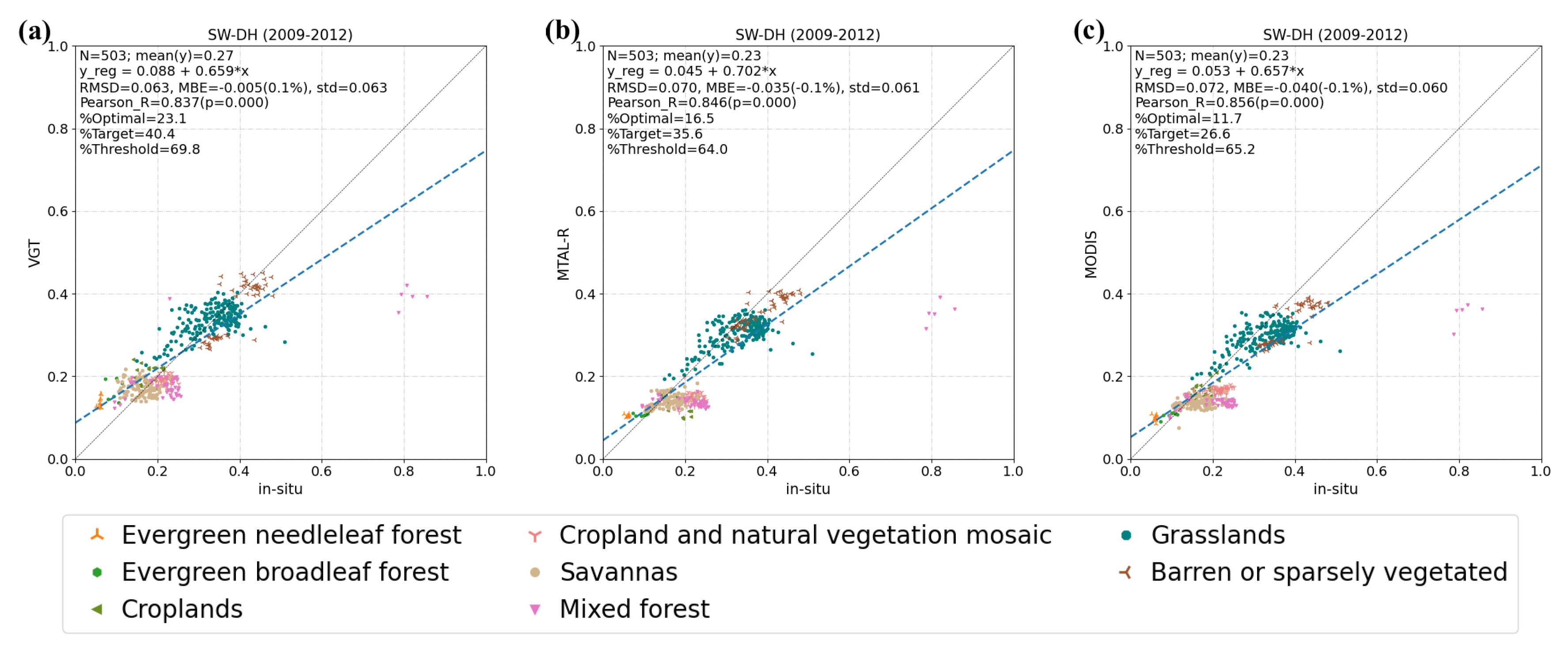
3.1.1. VGT versus Ground Measurements, Indirect Comparison with MODIS and MTAL

In Figure 4, time series are displayed for four stations that were chosen because they produced ground measurements over the full four-year period. One observes that VGT agrees well with the ground data and even provides the best scores in terms of the RMSD as compared with MODIS and MTAL-R except for Agoufou. The seasonality is also captured by the satellite products reasonably well. For these plots, only those dates that provided concomitant data for all three satellites products and ground measurements were considered. Other plots that included all data available were produced and are displayed in Appendix A. Similar conclusions can be drawn.

The more exhaustive time series presented in Figure A1a show that not only satellite albedo products can be contaminated by residual clouds but ground measurements can also be contaminated by artifacts (see the high values in September 2011). Note that the seasonality is much better characterised by the satellite products.

Further accuracy analyses were done by combining all ground measurements available. The scatter plots presented in Figure 5 were produced using ground measurements from the stations listed in Table 3 with measurements available throughout the study period (2009–2012). Again, only those dates that provided concomitant data for all three satellites products and ground measurements were considered. The counterpart plots featuring all data available over the same period are provided in Appendix A. Including all these stations allowed us to widen the range of the land cover types considered, with a total of eight IGBP classes (among the 17 possible categories) represented. Figure 5 reveals similar distribution patterns for the three satellite products. In particular, data that are tagged mixed forest are well off the 1:1 line (especially when they are covered by snow), while those tagged barren or sparsely vegetated show good agreement between ground measurements and satellite data. The discrepancies between ground measurements and satellite estimates for mixed forest covered by snow (pink triangles with in situ albedo larger than 0.5) are potentially due to representativeness issues (footprints are between 40 and 900 m in diameter, depending on the tower height for ground measurements, while they are around 1 km for satellite estimates), which could explain part of the overestimation of ground measurements compared with satellite estimates. All results displayed in Figure 5 and Figure A2 are summarized in

Table 8. Accuracy assessment of VGT, MTAL-R and MODIS surface albedo satellite products versus ground measurements coming from GBOV, AMMA and BSRN stations during the 1 January 2009–31 December 2012 period when those dates that provided concomitant data for all three satellites products and ground measurements were considered (left) or simply using all data available (right). Absolute MBE are calculated over albedo values less 0.15 while relative MBE (in %) are calculated over albedo values greater than 0.15.

		Only Concomitant Data			All Available Data
		VGT	MTAL-R	MODIS	VGT	MTAL-R	MODIS
N		503	503	503	784	1199	922
mean(y)		0.27	0.23	0.23	0.25	0.23	0.22
RMSD		0.063	0.070	0.072	0.068	0.085	0.090
MBE	AL ≤ 0.15	−0.005	−0.035	−0.040	−0.002	−0.029	−0.044
	AL > 0.15	(0.1%)	(−0.1%)	(−0.1%)	(0.1%)	(0.0%)	(−0.1%)
STD		0.063	0.061	0.060	0.068	0.080	0.078
R		0.837	0.846	0.856	0.799	0.784	0.766
Regression line	offset	0.088	0.045	0.053	0.089	0.083	0.074
	slope	0.659	0.702	0.657	0.636	0.566	0.561
Pass rates	%optimal	23.1	16.5	11.7	20.4	17.2	11.0
	%target	40.4	35.6	26.6	35.8	34.9	24.3
	%threshold	69.8	64.0	65.2	62.2	64.5	60.0

.

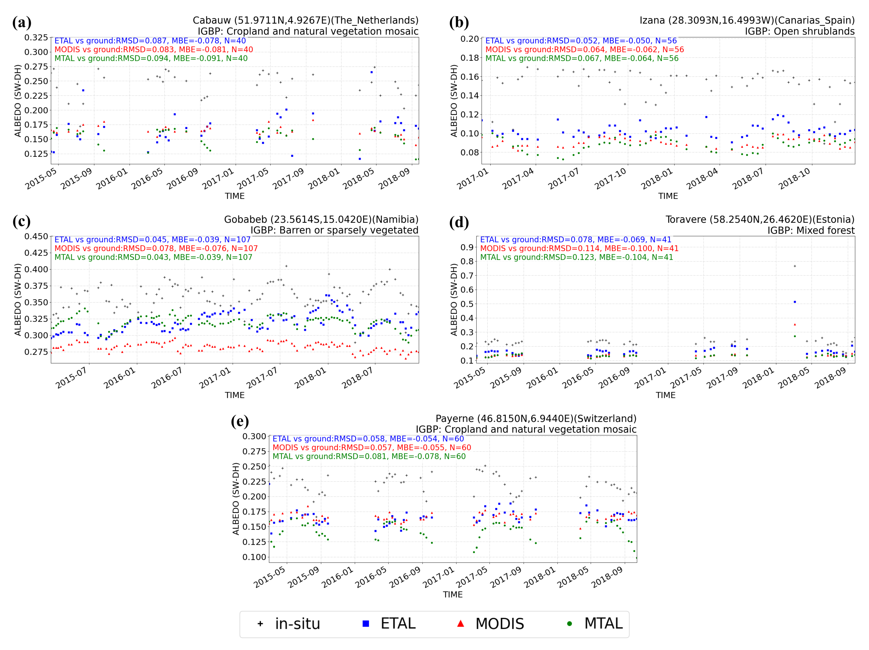
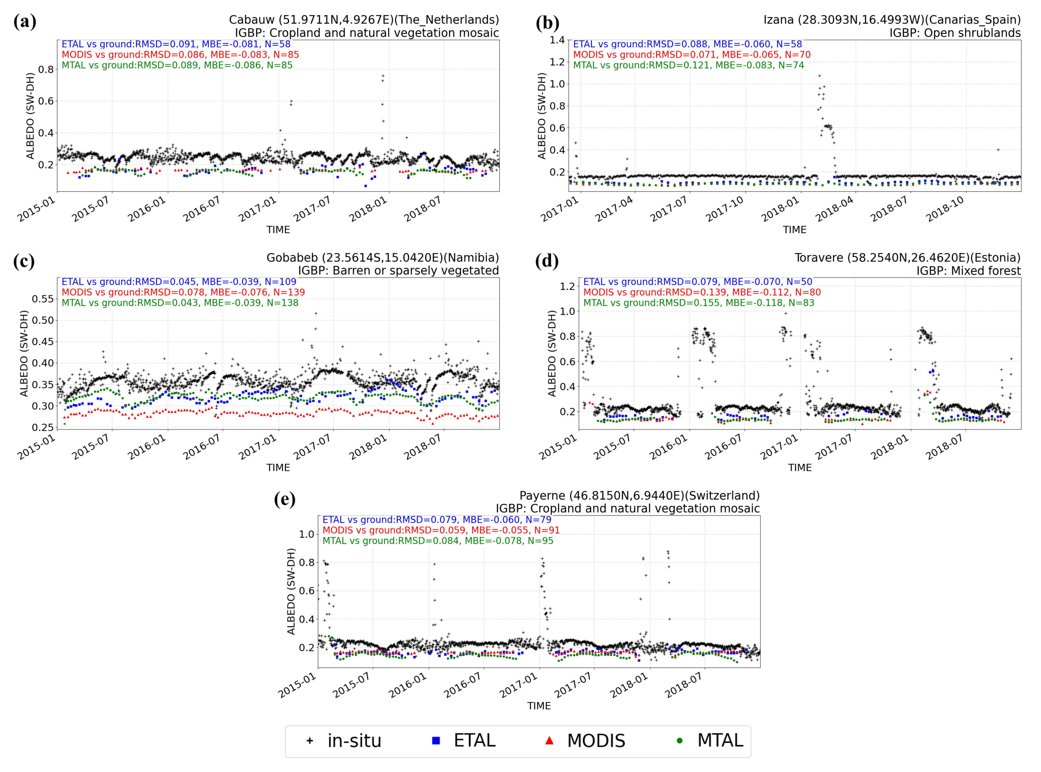
3.1.2. ETAL versus Ground Measurements, Indirect Comparison with MODIS and MTAL

The exercise in Section 3.1.1 was similarly applied to ETAL. In Figure 6, time series are displayed for five stations that were also chosen because they produced ground measurements throughout the full four-year period. ETAL agrees well with ground measurements and provides the best scores in terms of the MBE as compared with MODIS and MTAL-R. The seasonal cycle is not as marked as that in Figure 4. For these plots, only those dates that provided concomitant data for all three satellites products and ground measurements were considered. Other plots that included all data available were produced and are displayed in Appendix B. With the exception of Payerne, ETAL shows better MBE scores as compared with MODIS and MTAL.

The scatter plots displayed in Figure 7 were also produced using ground measurements from the stations listed in Table 3 with measurements available throughout the evaluation period (2015–2018). Again, only those dates that provided concomitant data for all three satellites products and ground measurements were considered. The counterpart plots featuring all data available over the same period are provided in Appendix B. A variety of land covers are therefore represented (8 in Figure 7 and 12 in Figure A4 IGBP classes among the 17 possible). Figure 7 reveals an agreement between ETAL and ground measurements, and the correspondence is comparable to the case of VGT in terms of RMSD (0.057 for ETAL and 0.063 for VGT). The patterns remain very similar for the three satellite products. The lower number of points in Figure A4b results from the lower number of stations available within the MSG disk (which covers only Europe, Africa and South America) during the period 2015–2018. All results displayed in Figure 7 and Figure A4 are summarized in

Table 9. Accuracy assessment of ETAL, MTAL and MODIS surface albedo satellite products versus ground measurements coming from GBOV, AMMA and BSRN stations during the 1 January 2015–31 December 2018 period when those dates that provided concomitant data for all three satellites products and ground measurements were considered (left) or simply using all data available (right). Absolute MBE are calculated over albedo values less 0.15 while relative MBE (in %) are calculated over albedo values greater than 0.15.

		Only Concomitant Data			All Available Data
		ETAL	MTAL	MODIS	ETAL	MTAL	MODIS
N		406	406	406	1135	732	1284
mean(y)		0.19	0.18	0.18	0.17	0.17	0.16
RMSD		0.057	0.070	0.070	0.073	0.083	0.073
MBE	AL ≤ 0.15	−0.035	−0.050	−0.053	−0.031	−0.047	−0.042
	AL > 0.15	(−0.1%)	(−0.2%)	(−0.2%)	(−0.1%)	(−0.1%)	(−0.1%)
STD		0.046	0.048	0.047	0.067	0.069	0.060
R		0.885	0.867	0.896	0.680	0.752	0.753
Regression line	offset	0.023	−0.001	0.030	0.065	0.048	0.049
	slope	0.746	0.784	0.640	0.528	0.560	0.556
Pass rates	%optimal	7.6	5.7	3.4	8.5	6.7	8.3
	%target	20.7	20.7	8.1	19.8	19.4	19.9
	%threshold	43.6	43.1	31.3	44.2	39.5	45.1

.

3.2. Temporal Analysis Per Land Cover Type: Phase 2

In the second phase of the evaluation, both products under test were inter-compared with MODIS over a large number of sites scattered around the world (Section 2.3) to cover a multitude of climate and land cover types. The strategy applied to derive surface albedo values at each site is presented in Section 2.5. After associating each site with a specific land cover, we were able to summarize our observations per land cover type. Here, we simply took the land cover type of the pixel closest to the site in the MODIS Land Cover product (5 km × 5 km of spatial resolution). The map represents the land cover condition in the year 2010.

3.2.1. VGT versus MODIS

Figure 8a,c,e presents time series of the mean surface albedo for both VGT and MODIS for three land cover types, viz. evergreen needleleaf forest, croplands and open shrublands, during the first time period (2009–2012). Hence, they concern three subsets of the 1019 sites. For each date, all VGT and MODIS surface albedo values associated with sites of the same land cover type are averaged. MBE and STD values of the differences (VGT-MODIS) are also calculated per land cover type and displayed in Figure 8b,d,f. The times series on the left-hand side show all the data available from each dataset, while the bias graphs on the right-hand side show only the bias for the matching dates. We observe a positive bias of VGT over MODIS (e.g., a mean MBE of 0.024 for Croplands) and higher standard deviations (std) over the winter months in the northern hemisphere. These higher std values are caused by the presence of increased biases for snowy events (bigger differences with higher albedo values), which, in our analyses, are visible during the November–February period since most of the analyzed stations are located in the northern hemisphere (winter months). We also note that smaller seasonal variations coincide with smaller standard deviation values (open shrublands as compared with the other two land cover types). Here, the seasonal patterns are more linked to the vegetation seasonal cycles. The results for the other land covers are presented in Appendix C.

One way to expand this quantitative approach is to look at the MBE (respectively, rMBE) for each site and compare it to the requirements in Table 5 to draw statistics per land cover type, which is the same approach taken in [23]. We obtained the results displayed in Figure 9 for all land covers. Both surface albedo regimes (above or below 0.15) are considered. Note that, while we only looked at the target requirement for surface albedo values lower than 0.15, we looked at both the target and threshold requirements for the other case since the more relaxed requirement substantially improves the results. Interestingly, some of the qualitative observations in Figure 5 are confirmed, viz. the high scores for barren or sparsely vegetated and the more moderate scores for mixed forest.

3.2.2. ETAL versus MODIS

The same strategy was applied for the inter-comparison of ETAL with respect to MODIS over the second time period, 2015–2018. Time series of the mean surface albedo values, as well as the MBE and STD of the differences (ETAL-MODIS) for the same three land cover types, as in Section 3.2.1, are displayed in Figure 10. For all three cases, we observe very low values for the mean MBE (values between 0 and −0.006), in agreement with the behavior of the mean ETAL and MODIS surface albedo values (see left-hand-side figures). The mean STD value retrieved for ETAL is also significantly smaller as compared with VGT for the type evergreen needleleaf forest (0.033 as compared with 0.048). Other land cover types are considered in Appendix D.

Similar to what was done for Figure 9, we summarize all results per land cover type in Figure 11. For the case with surface albedo lower than 0.15 (Figure 11a), we see that 11 out of 13 land cover types present pass rates beyond 80%. For the regime of surface albedo greater than 0.15, 10 out of 14 land cover types have pass rates beyond 50% for the threshold requirement. Overall, all land cover types give better results than those for VGT regardless of the albedo regime, except snow and ice, which concerns only two stations. Land covers of the type barren or sparsely vegetated, grasslands or open shrublands that often characterise desertic areas (Figure 2) have very high pass rates (beyond 80% for the target requirements).

3.3. Global-Scale Analysis: Phase 3

In Phase 3, the products were evaluated following a full-globe analysis. Density scatter plots are first examined to characterise the correlation globally between the test datasets (VGT or ETAL) and the reference dataset (MODIS).

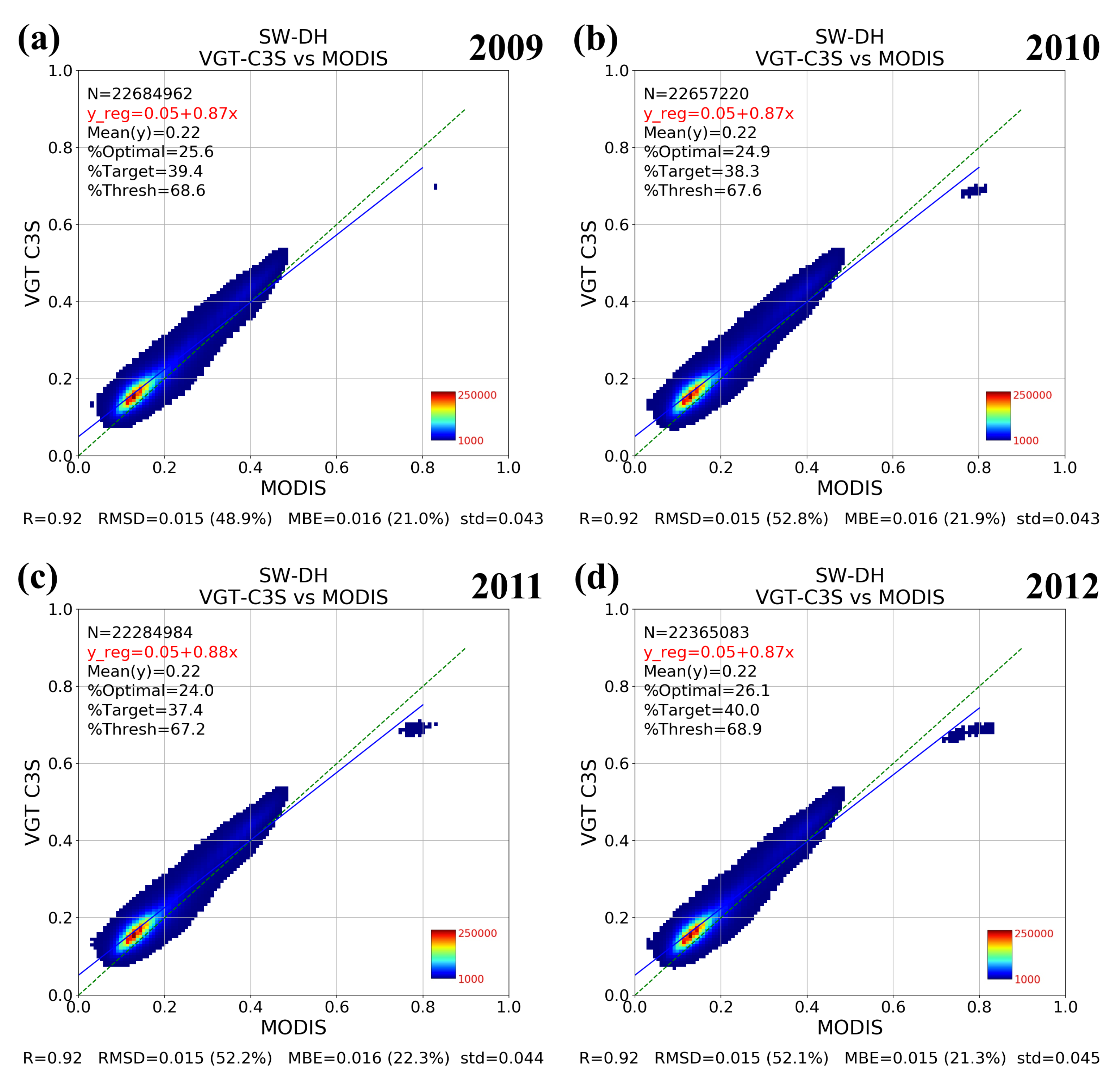
3.3.1. VGT versus MODIS

As expected from the prior analysis in Section 3.2.1, VGT overestimates the snow-free surface albedo as compared with MODIS, while it underestimates the snow surface albedo (patches with AL ≃ 0.8), as seen in Figure 12. In addition, we see no annual evolution in the VGT versus MODIS performances since the results from the four-year period are almost identical. On the one hand, the Pearson correlation coefficients are high (above 0.9 for all years), which indicates that both VGT and MODIS have the same seasonal pattern. On the other hand, the pass rates remain poor because of the bias between the two products. At best, the threshold requirement reaches 68.9% in 2018. These rates are simply calculated by comparing the bias (respectively, relative bias) between VGT and MODIS surface albedos for all the pixels tested and for all dates with respect to the requirements in Table 5. The performance statistics are compiled in

Table 10. Performance statistics between VGT versus MODIS products during the overlap period (2009–2012). Absolute MBE and RMSD are calculated over albedo values less 0.15 while relative MBE and RMSD (in %) are calculated over albedo values greater than 0.15.

		VGT vs. MODIS
		2009	2010	2011	2012
Correlation (R)		0.92	0.92	0.92	0.92
Root-mean-square deviation (RMSD)	AL ≤ 0.15	0.015	0.015	0.015	0.015
	AL > 0.15	(48.9%)	(52.8%)	(52.2%)	(52.1%)
Mean bias error (MBE)	AL ≤ 0.15	0.016	0.016	0.016	0.015
	AL > 0.15	(21.0%)	(21.9%)	(22.3%)	(21.3%)
Standard deviation (STD)		0.043	0.043	0.044	0.045
Linear regression line	offset	0.05	0.05	0.05	0.05
	slope	0.87	0.87	0.88	0.87
Pass rates	%optimal	25.6	24.9	24.0	26.1
	%target	39.4	38.3	37.4	40.0
	%threshold	68.6	67.6	67.2	68.9

.

3.3.2. ETAL versus MODIS

Similar to the approach in Section 3.3.1, the correlation between ETAL and MODIS is assessed over the full globe for the corresponding four-year period.

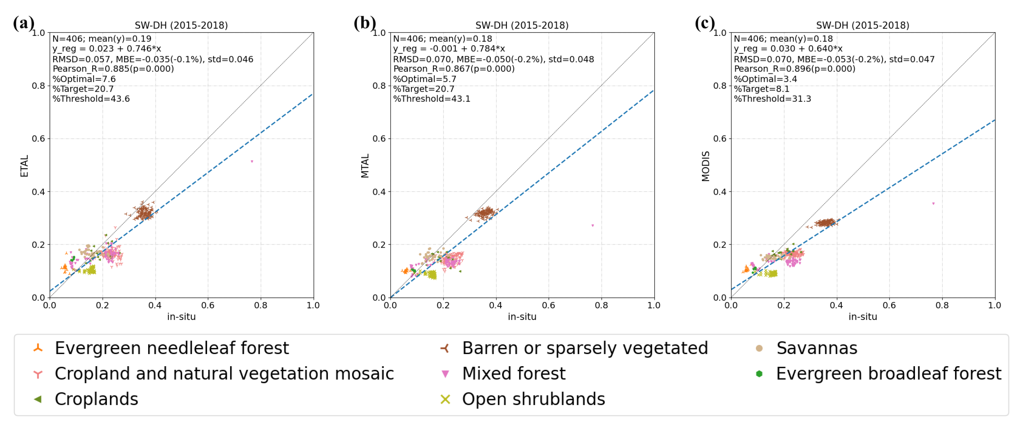
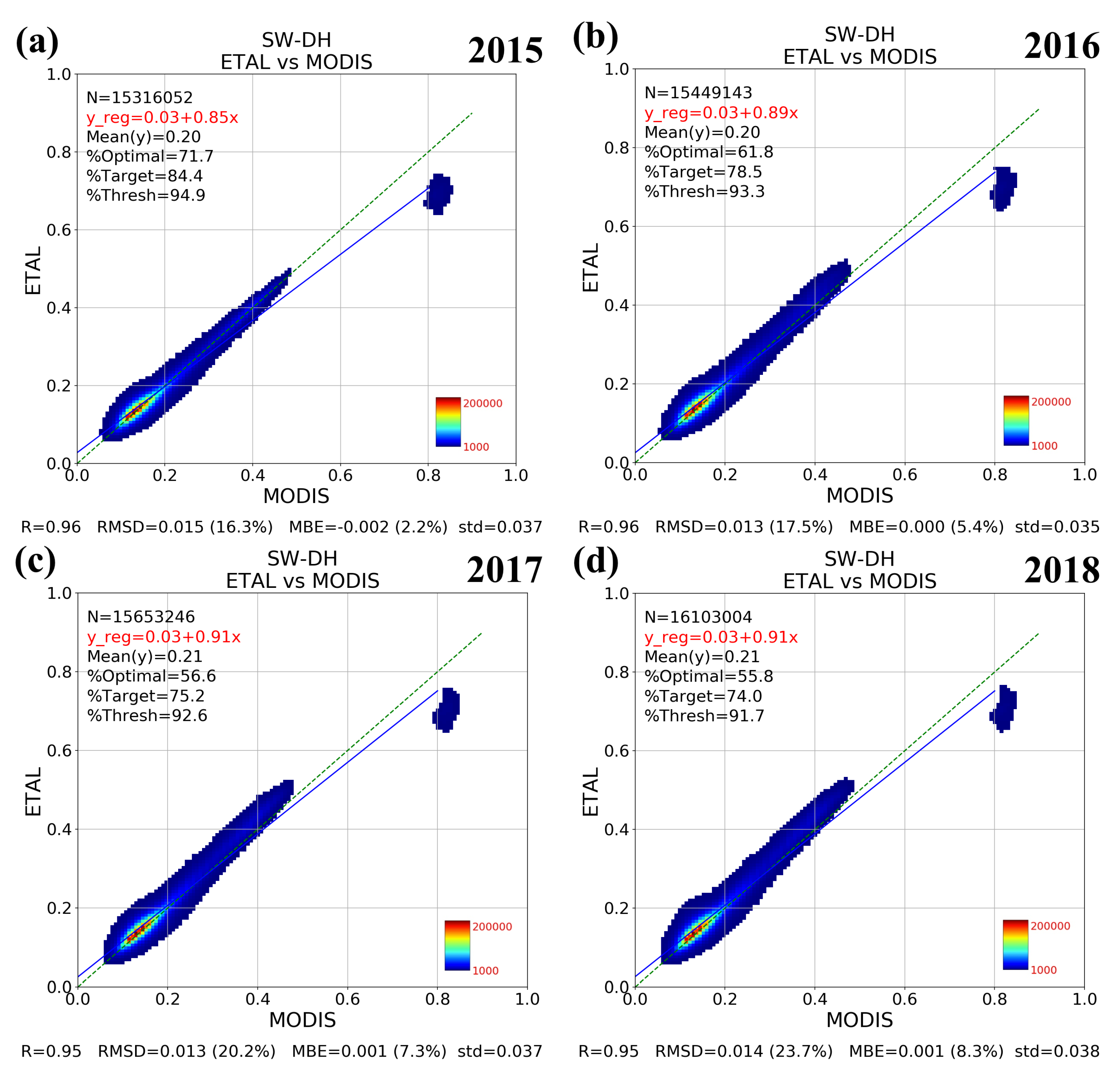
• Statistics of the differences
  Density scatter plots for each year are displayed in Figure 13. As expected from the observations in Section 3.2.2, ETAL and MODIS are very well correlated, with threshold pass rates beyond 90%, and the optimal pass rates for ETAL are also more than twice those of VGT. Standard deviation values of the differences are also substantially lower than in the VGT case. For the years 2016–2018, ETAL albedo values of around 0.3–0.4 are slightly higher compared with MODIS albedo values. Again, ETAL underestimates the snow albedo (AL ≃ 0.8) compared with MODIS, but, overall, there is a very good match between the two datasets. This can be seen from the weaker scattering of the pixels along the regression line compared with Figure 12. The performance statistics are compiled in

  Table 11. Performance statistics between ETAL versus MODIS products during the overlap period (2015–2018). Absolute MBE and RMSD are calculated over albedo values less 0.15 while relative MBE and RMSD (in %) are calculated over albedo values greater than 0.15.

  		ETAL vs. MODIS
  		2015	2016	2017	2018
  Correlation (R)		0.96	0.96	0.95	0.95
  Root-mean-square deviation (RMSD)	AL ≤ 0.15	0.015	0.013	0.013	0.014
  	AL > 0.15	(16.3%)	(17.5%)	(20.2%)	(23.7%)
  Mean bias error (MBE)	AL ≤ 0.15	−0.002	0.000	0.001	0.001
  	AL > 0.15	(2.2%)	(5.4%)	(7.3%)	(8.3%)
  Standard deviation (STD)		0.037	0.035	0.037	0.038
  Linear regression line	offset	0.03	0.03	0.03	0.03
  	slope	0.85	0.89	0.91	0.91
  Pass rates	%optimal	71.7	61.8	56.6	55.8
  	%target	84.4	78.5	75.2	74.0
  	%threshold	94.9	93.3	92.6	91.7

  .

  Figure 13. Density scatter plots for the inter-comparison of ETAL versus MODIS for: (a) 2015; (b) 2016; (c) 2017; and (d) 2018. To maintain a reasonable number of samples, a spatial subsampling of 1:10 is considered. The green dashed line is the 1:1 line, and the blue line is the regression line. Absolute MBE and RMSD are calculated over albedo values less 0.15 while relative MBE and RMSD (in %) are calculated over albedo values greater than 0.15.

  Figure 13. Density scatter plots for the inter-comparison of ETAL versus MODIS for: (a) 2015; (b) 2016; (c) 2017; and (d) 2018. To maintain a reasonable number of samples, a spatial subsampling of 1:10 is considered. The green dashed line is the 1:1 line, and the blue line is the regression line. Absolute MBE and RMSD are calculated over albedo values less 0.15 while relative MBE and RMSD (in %) are calculated over albedo values greater than 0.15.
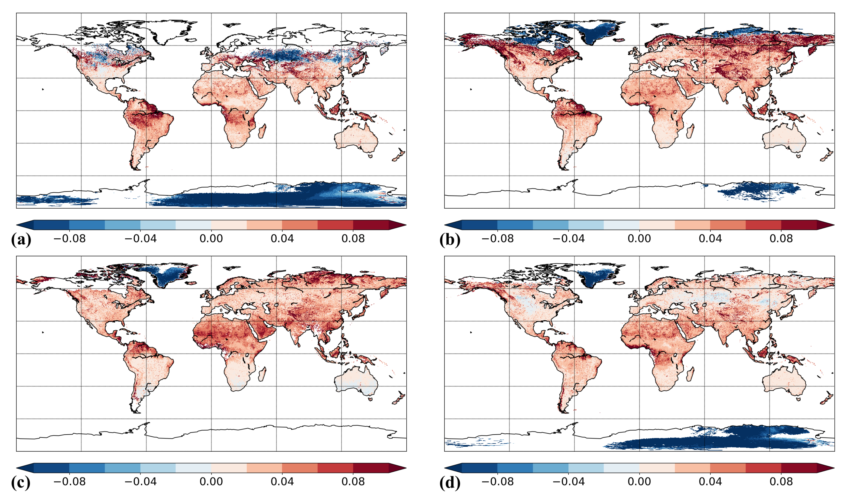
• Global seasonal bias
  As indicated in Section 2.5, seasonal maps of the mean differences can be produced to infer temporal and spatial differences between both the test and reference products. The results for ETAL are provided in Figure 14. Overall, one sees that the bias is relatively stable over the seasons. However, a few interesting observations can be mentioned here:

  -

  Regions affected by snow have a strong negative bias in winter (underestimation of the snow surface albedo by ETAL in comparison with MODIS, as previously observed) and a positive bias otherwise (e.g., Canada).

  -

  In agreement with our observations in Figure 13, desertic areas (for example, the Sahara) where surface albedo values range around 0.3 experience strong positive biases.

  -

  Over South America, the positive bias is greater during December-January-February (DJF) (southern hemisphere summer) in comparison with June-July-August (JJA) (southern hemisphere winter). Furthermore, the positive bias over rainforests is in agreement with Figure 11, which shows lower performances for evergreen forests, potentially because of persistent cloudiness over these regions.

  -

  Over northern Africa, the positive bias is greater during JJA (northern hemisphere summer) in comparison with DJF (northern hemisphere winter).

  -

  Over north-eastern Siberia, the positive bias is minimal during September-October-November (SON) (northern hemisphere fall).

  -

  Several regions experience low bias throughout the year including the southern part of South America, southern Africa, Australia as well as the southern part of the United States of America and Western Europe.

  Figure 14. Mean bias of the surface albedo (ETAL-MODIS) for the period from January 2015 to December 2018 for: (a) December-January-February; (b) March-April-May; (c) June-July-August; and (d) September-October-November periods. The white color indicates the absence of data (either missing or filtered at the preprocessing step).

  Figure 14. Mean bias of the surface albedo (ETAL-MODIS) for the period from January 2015 to December 2018 for: (a) December-January-February; (b) March-April-May; (c) June-July-August; and (d) September-October-November periods. The white color indicates the absence of data (either missing or filtered at the preprocessing step).

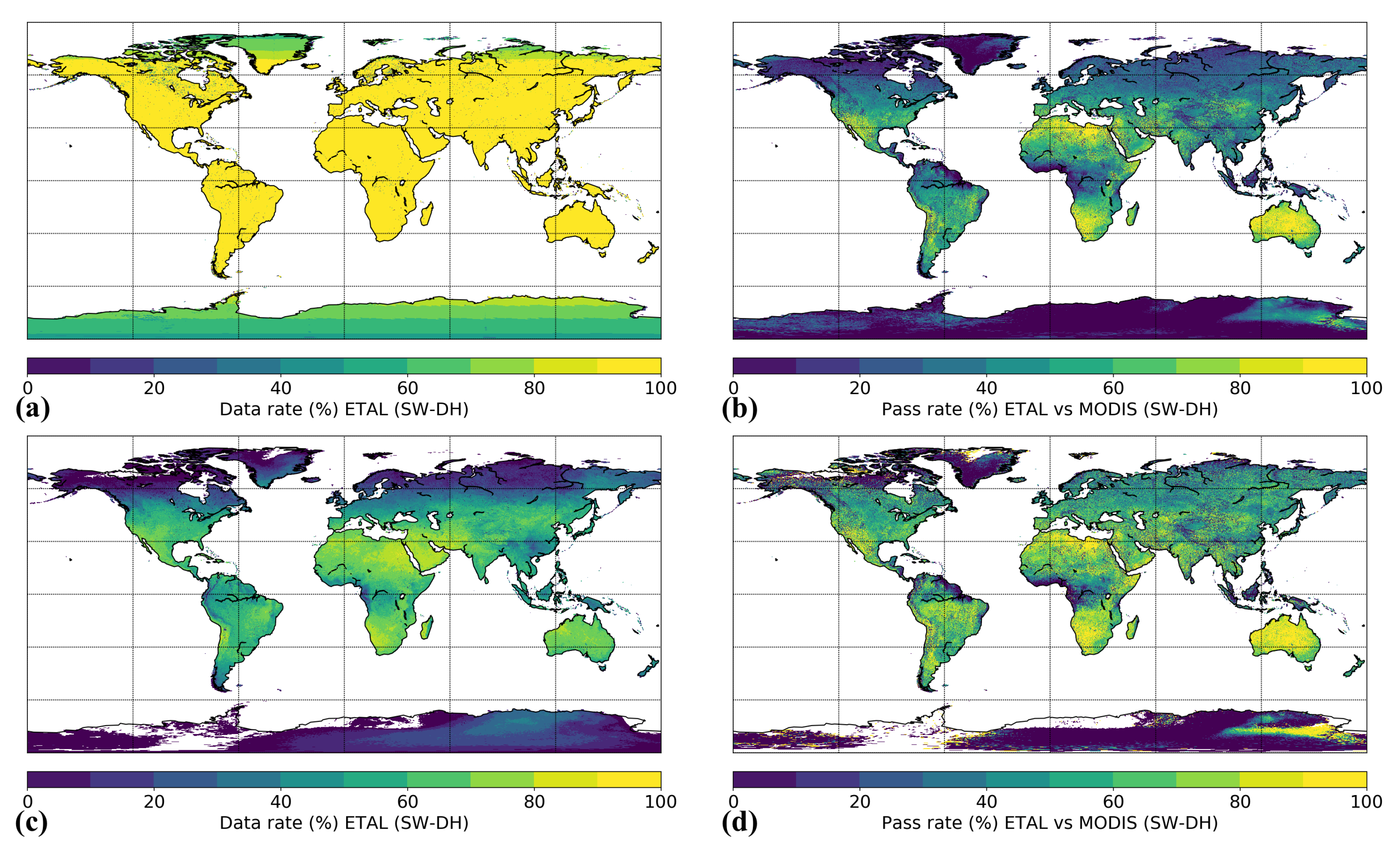
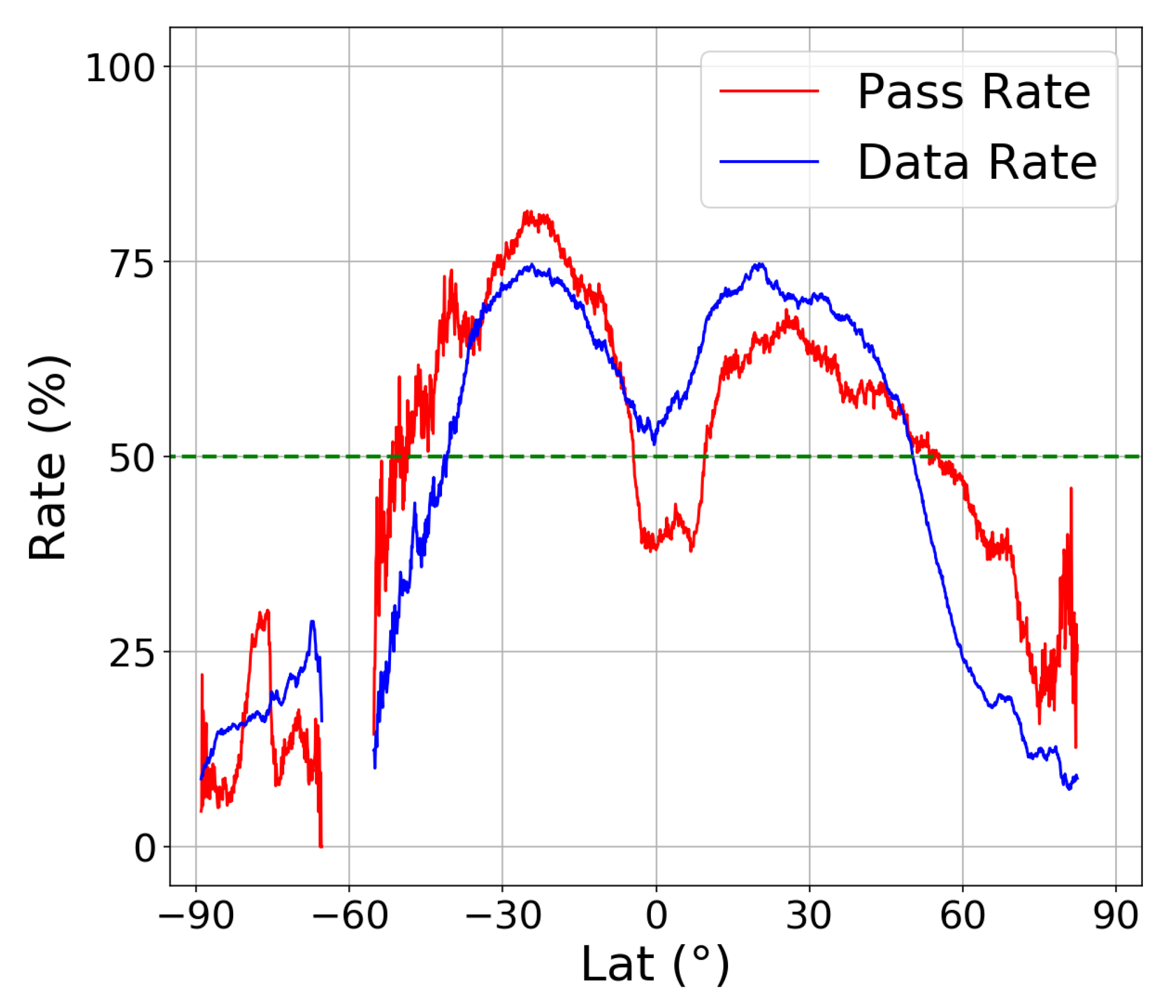
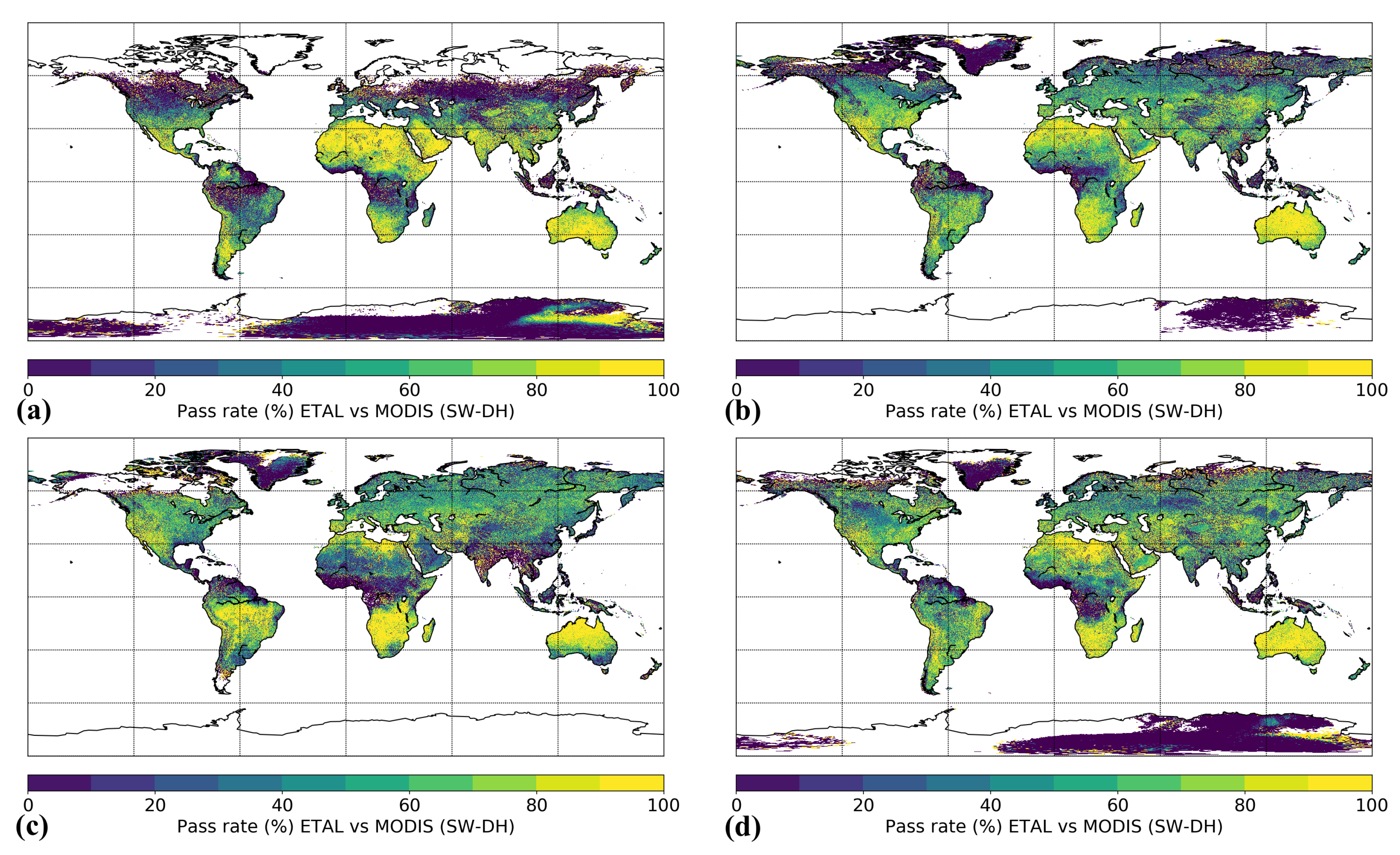
• Pass rate maps
  Another approach to quantifying the quality of ETAL (with respect to MODIS) over the full globe consists of assessing, on the one hand, its data rate (%) (or product temporal coverage) and, on the other hand, its pass rate (on the basis of the threshold requirement in Table 5) (%) for all pixels. The pass rate is defined as in Section 2.4. Figure 15 shows both the data rate and the pass rate for ETAL versus MODIS prior to filtering bad-quality surface albedo values and after filtering (referring to Section 2.5). Comparing Figure 15c and Figure 15a, one sees that many data are lost in the filtering process, particularly over tropical areas that belong to the inter-tropical convergence zone (ITCZ). In return, pass rates are substantially improved when good values (filtered data) are kept, as revealed by the differences over Siberia, Mexico and South America, among others (Figure 15d versus Figure 15b). This observation stresses the importance of the information distributed together with the albedo variables (quality flag, information about the age and uncertainties).
  Averaging the observations of both the data rates and pass rates (after filtering, Figure 15c,d) over the longitudes (for a given latitude) enables the construction of the rate profiles in Figure 16. It shows two maxima for the pass rate at about 25°S and 25°N, with a higher value of around 82% for the southern hemisphere one, unsurprisingly caused by the large high-pass-rate areas, viz., Australia and Southern Africa. We can also observe that from about 52°S to 52°N, the pass rate is over 50% on average, with a small band coinciding with the ITCZ zone (about 5°S to 10°N), where it falls to lower values of around 40%. The ETAL data rate, also shown in Figure 16, presents two peaks, both at about 75% roughly at 27°S and 20°N. After filtering (Section 2.5); more than 50% of ETAL data, on average, remain between 42°S and 50°N.

  Figure 15. Mean yearly ETAL data rate and ETAL pass rate with respect to MODIS over the period 2015–2018: (a,b) before pre-processing the data (filtering on the quality flag and other criteria); and (c,d) after filtering. The white color indicates the absence of data (either missing in (a,b) or filtered at the preprocessing step in (c,d)).

  Figure 15. Mean yearly ETAL data rate and ETAL pass rate with respect to MODIS over the period 2015–2018: (a,b) before pre-processing the data (filtering on the quality flag and other criteria); and (c,d) after filtering. The white color indicates the absence of data (either missing in (a,b) or filtered at the preprocessing step in (c,d)).

  Figure 16. Mean yearly ETAL data rate and ETAL versus MODIS pass rate averaged per latitude (after filtering with the preprocessing). Any latitude that did not have a minimum number of 10 pass rate values was discarded.

  Figure 16. Mean yearly ETAL data rate and ETAL versus MODIS pass rate averaged per latitude (after filtering with the preprocessing). Any latitude that did not have a minimum number of 10 pass rate values was discarded.
• Seasonal pass rate maps

Similar to the bias maps that were produced per season (Figure 14, where each season is composed of three consecutive months), seasonal pass rate maps were calculated. All four maps are presented in Figure 17. Unsurprisingly, areas with low bias values also present high pass rates, as is the case for Australia or Southern Africa over all periods. Over desertic areas (e.g., the Sahara) that have high surface albedo values (regimes, surface albedo above 0.15), the pass rate is also very high throughout the seasons. Overall, these maps reveal some spatial and temporal variabilities, including the surface albedo itself.

4. Discussion

This paper presents an evaluation exercise of VGT (C3Sv1) and ETAL surface albedo products, which were released recently. The evaluation was performed in three phases including direct point-to-pixel comparisons (Phase 1) and indirect validations (Phases 1–3). It consisted of inter-comparisons of VGT and ETAL surface albedo data both at a local scale over 33 ground measurement stations and worldwide with two independent operational satellite products (MTAL-NRT plus MTAL-R and MODIS).

In accordance with the prescription from the joint Committee on Earth Observation Satellites (CEOS), shortwave directional-hemispherical (SW-DH) quantities were used for satellite-based surface albedo data since they cover the full solar spectrum. To cope with the spatial and temporal variabilities in surface albedo, our inter-comparisons were performed at local and global scales for data from two distinct four-year periods, for which we had the maximum amount of satellite data available (2009–2012 for VGT and 2015–2018 for ETAL). Information about the land cover type in 2010 (from the MODIS Land Cover product) was also considered in our analyses.

In Phase 1, VGT and ETAL satellite data were compared with ground measurements collected at 33 ground stations from different networks (with worldwide coverage) that cover different climate zones. The nearest-neighbor satellite pixel, as seen from the station, was used to infer satellite surface albedo values. In this way, one could derive equivalent time series for both the satellite products and the ground measurements. Furthermore, other accuracy analyses could be performed per land cover type using the land cover information of the ground station. Our qualitative inspections revealed that both the VGT and ETAL satellite data agree well with the other satellite data, as well as the ground measurements. The seasonal cycles are faithfully reproduced (e.g., Figure 4). Our further accuracy analyses revealed that both VGT and ETAL agree well with the behavior of other satellite products when assessed per land cover type.

In Phase 2, VGT and ETAL products were tested against MODIS over a large number of sites (1019), chosen for the sake of spatial coverage as the AERONET stations. Having resampled MODIS to cope with the VGT grid (equirectangular projection with 1/112° × 1/112° spatial resolution) and the ETAL grid (sinusoidal projection with 0.01° × 0.01° spatial resolution), we calculated equivalent surface albedo values for all satellite products to infer time series. Visual inspections revealed a systematic overestimation of the surface albedo by VGT as compared with MODIS by approximately 0.02, while the match between ETAL and MODIS is a lot stronger (mean MBE below 0.01). Including two accuracy indications prescribed (in the frame of the LSA-SAF project) for two regimes of surface albedo values (see Table 5) and information about the land cover type enabled us to derive pass rates per land cover type for both satellite products. The results were significant for ETAL (Figure 11) as compared with VGT (Figure 9), with 11 out 13 land cover types giving pass rates beyond 80% for the regime of surface albedo less than 0.15 (compared with none for VGT) and 10 out 14 land cover types giving pass rates beyond 50% for the regime of surface albedo more than 0.15 (compared with 5 for VGT).

In Phase 3, a global (pixel-by-pixel) analysis was performed for both four-year periods. The observations from Phase 1 and 2 were confirmed. We observe that, despite high (Pearson) correlation coefficients (beyond 0.9), VGT overestimates the surface albedo as compared with MODIS by about 0.02 in absolute value for the regime of surface albedo less than 0.15 and by about 22% in relative value for albedo values greater than 0.15. The RMSD in absolute value is about 0.015 for albedo values less than 0.15, and 51.5% in relative value for albedo values greater than 0.15. In contrast, the bias for ETAL when compared with MODIS remains very small. Over the other four-year period, one finds that ETAL overestimates the surface albedo as compared with MODIS by 0.001 in absolute value for the regime of surface albedo less than 0.15 and by about 5.8% in relative value for albedo values greater than 0.15. The RMSD in absolute value is about 0.014 for albedo values less than 0.15 and 19.4% in relative value for albedo values greater than 0.15. Spatially, we observe an overestimation of the surface albedo by ETAL as opposed to MODIS, except in polar regions (snow pixels), where it is the opposite. The discrepancy between ETAL and MODIS products increases over mountainous areas (Himalaya) and other regions, such as the Amazon basin and the Congo basin. Moreover, we show that full characterization (completeness and accuracy) of the product quality (with respect to MODIS) is elegantly done by joining full-globe data rate maps and full-globe pass rate maps. After filtering the data on the basis of quality information, we observe lower data rates over cloudy areas (such as those on the ITCZ mentioned above) and higher pass rates. Averaging the pass rates over the longitudes, we observe that, from about 52°S to 52°N, the pass rate is over 50% on average, with a small band coinciding with the ITCZ zone (about 5°S to 10°N), where it falls to lower values of around 40% and average values as high as 82% around 25°S. The use of seasonal pass rate maps reveals the spatial and temporal variability of ETAL quality (as compared with MODIS). For example, over northern Europe and Siberia, pass rates are higher in JJA than any other season while at the same time southeastern Australia experiences its lowest pass rate values.

Different elements in the retrieval methodology contribute to the mismatches between the three satellite products under study (C3Sv1 VGT, ETAL and MODIS MCD43D51 C6). First, atmospheric correction is performed with a climatology (on the basis of the Copernicus Atmosphere Monitoring Service, CAMS) for the aerosol contribution in ETAL, while MODIS uses its own daily aerosol product ([49]) and VGT uses MERRA-2 (the Modern-Era Retrospective analysis for Research and Applications, Version 2) reanalyses. This can result in important mismatches wherever important concentrations of aerosols are found.

In addition, the performance of the BRDF model for good clear-sky observations is dependent on the number of available looks during the synthesis period as well as the distribution of the angular sampling. Besides, large BRDF uncertainties are associated to snow targets, for which the RTLSR model [44] used by all three products is not well suited [55].

The different compositing periods (20 days for C3Sv1 VGT and ETAL and 16 days for MODIS) could also induce mismatches between the products especially in places with fast-varying environments (polar regions, mountains and forests).

Concerning the main input data, it should be noted that three sensors have different spectral bands (see Table 1). While both C3Sv1 VGT and MODIS albedo products ingest blue channels (both of them similar), this band is not available in AVHRR used by ETAL. Besides, ETAL red and NIR channels are wider than the other sensors with MODIS presenting the most narrow bandwidth. In either case, all three products have comparable central wavelengths. Lastly, C3Sv1 VGT SWIR channel is the widest of all three and MODIS is again the most narrow while positioned over larger wavelengths as compared to ETAL. These differences could translate into reflectance mismatches in regions with high absorption features where large uncertainty values were found between pair of products.

Other factors include the field of view of the satellite, calibration errors and the spectral-to-broadband albedo conversion since the DH broadband albedos are defined using slightly different spectral regions (C3Sv1 VGT and ETAL both cover the band [0.3–4.0 $\mathsf{\mu }$ m] while the range is slightly wider for MODIS, [0.3–5.0 $\mathsf{\mu }$ m]) [36].

5. Conclusions

This paper presents an exhaustive validation for two new surface albedo datasets. The worldwide coverage and the long time span of the analyses contribute to the novelty of this work.

The methodology applied throughout the paper complies with the best practices for validation of global albedo satellite products of the CEOS/LPV group [32], whereby direct and indirect validation steps are needed.

In the direct validation part, it appeared that both VGT and ETAL agree well with the ground measurements considered as well as the other satellite products for either types of biome.

When addressing the indirect aspect of the validation, one confronted the results to requirements derived from users’ needs; viz., for VGT and ETAL albedo values below 0.15, we expect an MBE of less than 0.015 with respect to the reference data (MTAL-R plus MTAL-NRT and MODIS), while for VGT and ETAL albedo values above 0.15, the relative bias error should be less than 10%. The validation exercise presented here shows that these target requirements are almost achieved for VGT (0.02 of MBE and 22% of relative MBE with respect to MODIS) and exceeded for ETAL (0.001 of MBE and 5.8% of relative MBE with respect to MODIS) on a pixel-by-pixel basis over the two four-year periods considered.

Because the scientific algorithms for the retrieval of the surface albedo are similar for both products, two reasons can explain the lower performance of VGT: (1) the difference in the atmospheric correction between VGT, ETAL and MODIS products; and (2) the bias in the calibration of the VGT sensor, which would explain the degradation in product performance. This will require further investigations. With a retrieval method that is close to the MODIS algorithm, the ETAL albedo dataset demonstrates a very good correspondence with MODIS albedo products. This makes ETAL a good candidate for ensuring service continuity after the end of operation of the MODIS sensors.

References

- Pachauri, R.K.; Allen, M.R.; Barros, V.R.; Broome, J.; Cramer, W.; Christ, R.; Church, J.A.; Clarke, L.; Dahe, Q.; Dasgupta, P.; et al. Climate Change 2014: Synthesis Report. Contribution of Working Groups I, II and III to the Fifth Assessment Report of the Intergovernmental Panel on Climate Change; IPCC: Geneva, Switzerland, 2014. [Google Scholar]
- Bojinski, S.; Verstraete, M.; Peterson, T.C.; Richter, C.; Simmons, A.; Zemp, M. The Concept of Essential Climate Variables in Support of Climate Research, Applications, and Policy. Bull. Am. Meteorol. Soc. 2014, 95, 1431–1443. [Google Scholar] [CrossRef]
- GCOS-154. Systematic Observation Requirements for Satellite-Based Data Products for Climate: Supplemental Details to the Satellite-Based Component of the “Implementation Plan for the Global Observing System for Climate in Support of the UNFCCC (2010 Update); GCOS Rep. 154; WMO: Geneva, Switzerland, 2011; 138p, Available online: www.wmo.int/pages/prog/gcos/Publications/gcos-154.pdf (accessed on 10 June 2020).
- Coakley, J. Reflectance and Albedo, Surface in Encyclopedia of Atmospheric Sciences; Holton, J., Pyle, J., Curry, J., Eds.; Elsevier: Amsterdam, The Netherlands, 2003. [Google Scholar]
- Liang, S. Quantitative Remote Sensing of Land Surfaces; John Wiley & Sons: Hoboken, NJ, USA, 2005; Volume 30. [Google Scholar]
- Dickinson, R.E. Land processes in climate models. Remote Sens. Environ. 1995, 51, 27–38. [Google Scholar] [CrossRef]
- Dickinson, R.E. Land Surface Processes and Climate—Surface Albedos and Energy Balance. Adv. Geophys. 1983, 25, 305–353. [Google Scholar] [CrossRef]
- Wei, X.; Hahmann, A.N.; Dickinson, R.E.; Yang, Z.L.; Zeng, X.; Schaudt, K.J.; Schaaf, C.B.; Strugnell, N. Comparison of albedos computed by land surface models and evaluation against remotely sensed data. J. Geophys. Res. Atmos. 2001, 106, 20687–20702. [Google Scholar] [CrossRef]
- Ramanathan, V.; Barkstrom, B.R.; Harrison, E.F. Climate and the Earth’s radiation budget. AIP Conf. Proc. 1992, 247, 55–77. [Google Scholar] [CrossRef]
- Ferranti, L.; Viterbo, P. The European Summer of 2003: Sensitivity to Soil Water Initial Conditions. J. Clim. 2006, 19, 3659–3680. [Google Scholar] [CrossRef] [Green Version]
- Trigo, I.F.; Dacamara, C.C.; Viterbo, P.; Roujean, J.L.; Olesen, F.; Barroso, C.; Camacho-de Coca, F.; Carrer, D.; Freitas, S.C.; Garcia-Haro, J.; et al. The satellite application facility for land surface analysis. Int. J. Remote Sens. 2011, 32, 2725–2744. [Google Scholar] [CrossRef]
- Gueymard, C.A.; Lara-Fanego, V.; Sengupta, M.; Xie, Y. Surface albedo and reflectance: Review of definitions, angular and spectral effects, and intercomparison of major data sources in support of advanced solar irradiance modeling over the Americas. Sol. Energy 2019, 182, 194–212. [Google Scholar] [CrossRef]
- Csiszar, I.; Gutman, G. Mapping global land surface albedo from NOAA AVHRR. J. Geophys. Res. Atmos. 1999, 104, 6215–6228. [Google Scholar] [CrossRef]
- Strugnell, N.C.; Lucht, W. An algorithm to infer continental-scale albedo from AVHRR data, land cover class, and field observations of typical BRDFs. J. Clim. 2001, 14, 1360–1376. [Google Scholar] [CrossRef]
- Leroy, M.; Deuzé, J.; Bréon, F.; Hautecoeur, O.; Herman, M.; Buriez, J.; Tanré, D.; Bouffies, S.; Chazette, P.; Roujean, J. Retrieval of atmospheric properties and surface bidirectional reflectances over land from POLDER/ADEOS. J. Geophys. Res. Atmos. 1997, 102, 17023–17037. [Google Scholar] [CrossRef]
- Schaaf, C.B.; Gao, F.; Strahler, A.H.; Lucht, W.; Li, X.; Tsang, T.; Strugnell, N.C.; Zhang, X.; Jin, Y.; Muller, J.P.; et al. First operational BRDF, albedo nadir reflectance products from MODIS. Remote Sens. Environ. 2002, 83, 135–148. [Google Scholar] [CrossRef] [Green Version]
- Ba, M.B.; Nicholson, S.E.; Frouin, R. Satellite-derived surface radiation budget over the African continent. Part II: Climatologies of the various components. J. Clim. 2001, 14, 60–76. [Google Scholar] [CrossRef]
- He, T.; Liang, S.; Wang, D.; Shi, Q.; Tao, X. Estimation of high-resolution land surface shortwave albedo from AVIRIS data. IEEE J. Sel. Top. Appl. Earth Obs. Remote Sens. 2014, 7, 4919–4928. [Google Scholar] [CrossRef]
- Franchistéguy, L.; Geiger, B.; Roujean, J.L.; Samain, O. Retrieval of land surface albedo over France using SPOT4/VEGETATION data. In Proceedings of the 2nd International VEGETATION User Conference, Antwerp, Belgium, 24–26 March 2004; EUR 21552 EN. Antwerp, F., Veroustraete, E., Bartholomé, W., Verstraeten, W., Eds.; Office for Official Publications of the European Communities: Luxembourg, 2005; pp. 57–62. [Google Scholar]
- Dominique, C.; Bruno, S.; Xavier, C.; Jean-Louis, R.; Roselyne, L. Copernicus Global Land Operations Vegetation and Energy CGLOPS-1, Framework Service Contract 199494; Algorithm Theoretical Basis Document, Issue 2.11. 2018. Available online: https://land.copernicus.eu/global/sites/cgls.vito.be/files/products/CGLOPS1_ATBD_SA1km-V1_I2.11.pdf (accessed on 10 June 2020).
- Wang, D.; Liang, S.; He, T.; Yu, Y. Direct estimation of land surface albedo from VIIRS data: Algorithm improvement and preliminary validation. J. Geophys. Res. Atmos. 2013, 118, 12577–12586. [Google Scholar] [CrossRef]
- He, T.; Liang, S.; Wu, H.; Wang, D. Prototyping GOES-R albedo algorithm based on modis data. In Proceedings of the 2011 IEEE International Geoscience and Remote Sensing Symposium, Vancouver, BC, Canada, 24–29 July 2011; pp. 4261–4264. [Google Scholar] [CrossRef]
- Carrer, D.; Moparthy, S.; Lellouch, G.; Ceamanos, X.; Pinault, F.; Freitas, S.C.; Trigo, I.F. Land Surface Albedo Derived on a Ten Daily Basis from Meteosat Second Generation Observations: The NRT and Climate Data Record Collections from the EUMETSAT LSA SAF. Remote Sens. 2018, 10, 1262. [Google Scholar] [CrossRef] [Green Version]
- Muller, J.P.; López, G.; Watson, G.; Shane, N.; Kennedy, T.; Yuen, P.; Lewis, P.; Fischer, J.; Guanter, L.; Domench, C.; et al. The ESA GlobAlbedo project for mapping the Earth’s land surface albedo for 15 years from European sensors. In Proceedings of the IEEE Geoscience and Remote Sensing Symposium (IGARSS), Munich, Germany, 22–27 July 2012. [Google Scholar]
- Muller, J.P. GlobAlbedo Final Validation Report; University College London: London, UK, 2013; Available online: http://www.globalbedo.org/docs/GlobAlbedo_FVR_V1_2_web.pdf (accessed on 10 June 2020).
- Liang, S.; Zhao, X.; Liu, S.; Yuan, W.; Cheng, X.; Xiao, Z.; Zhang, X.; Liu, Q.; Cheng, J.; Tang, H.; et al. A long-term Global LAnd Surface Satellite (GLASS) data-set for environmental studies. Int. J. Digit. Earth 2013, 6, 5–33. [Google Scholar] [CrossRef]
- VGT Surface Albedo 10-Daily Gridded Data from 1981 to Present. Available online: https://cds.climate.copernicus.eu/cdsapp#!/dataset/satellite-albedo?tab=doc (accessed on 10 June 2020).
- Carrer, D.; Lellouch, G.; Pinault, F. ATBD for Ten-Day Surface Albedo from EPS/Metop/AVHRR (ETAL). 2018. Available online: https://landsaf.ipma.pt/GetDocument.do?id=756 (accessed on 10 June 2020).
- Nightingale, J.; Mittaz, J.P.; Douglas, S.; Dee, D.; Ryder, J.; Taylor, M.; Old, C.; Dieval, C.; Fouron, C.; Duveau, G.; et al. Ten priority science gaps in assessing climate data record quality. Remote Sens. 2019, 11, 986. [Google Scholar] [CrossRef] [Green Version]
- Román, M.O.; Schaaf, C.B.; Woodcock, C.E.; Strahler, A.H.; Yang, X.; Braswell, R.H.; Curtis, P.S.; Davis, K.J.; Dragoni, D.; Goulden, M.L.; et al. The MODIS (Collection V005) BRDF/albedo product: Assessment of spatial representativeness over forested landscapes. Remote Sens. Environ. 2009, 113, 2476–2498. [Google Scholar] [CrossRef] [Green Version]
- Román, M.O.; Schaaf, C.B.; Lewis, P.; Gao, F.; Anderson, G.P.; Privette, J.L.; Strahler, A.H.; Woodcock, C.E.; Barnsley, M. Assessing the coupling between surface albedo derived from MODIS and the fraction of diffuse skylight over spatially-characterized landscapes. Remote Sens. Environ. 2010, 114, 738–760. [Google Scholar] [CrossRef]
- Wang, Z.; Schaaf, C.; Lattanzio, A.; Carrer, D.; Grant, I.; Román, M.; Camacho, F.; Yu, Y.; Sánchez-Zapero, J.; Nickeson, J. Global Surface Albedo Product Validation Best Practices Protocol. Version 1.0. In Best Practice for Satellite Derived Land Product Validation: Land Product Validation Subgroup (WGCV/CEOS); Wang, Z., Nickeson, J., Román, M., Eds.; Land Product: Božice, Czech Republic, 2019; p. 45. [Google Scholar] [CrossRef]
- Taberner, M.; Pinty, B.; Govaerts, Y.; Liang, S.; Verstraete, M.M.; Gobron, N.; Widlowski, J.L. Comparison of MISR and MODIS land surface albedos: Methodology. J. Geophys. Res. Atmos. 2010, 115. [Google Scholar] [CrossRef] [Green Version]
- Pinty, B.; Taberner, M.; Haemmerle, V.R.; Paradise, S.R.; Vermote, E.; Verstraete, M.M.; Gobron, N.; Widlowski, J.L. Global-Scale Comparison of MISR and MODIS Land Surface Albedos. J. Clim. 2011, 24, 732–749. [Google Scholar] [CrossRef] [Green Version]
- Martonchik, J.V.; Diner, D.J.; Pinty, B.; Verstraete, M.M.; Myneni, R.B.; Knyazikhin, Y.; Gordon, H.R. Determination of land and ocean reflective, radiative, and biophysical properties using multiangle imaging. IEEE Trans. Geosci. Remote Sens. 1998, 36, 1266–1281. [Google Scholar] [CrossRef]
- Carrer, D.; Roujean, J.; Meurey, C. Comparing Operational MSG/SEVIRI Land Surface Albedo Products From Land SAF With Ground Measurements and MODIS. IEEE Trans. Geosci. Remote Sens. 2010, 48, 1714–1728. [Google Scholar] [CrossRef]
- Lattanzio, A.; Fell, F.; Bennartz, R.; Trigo, I.F.; Schulz, J. Quality assessment and improvement of the EUMETSAT Meteosat Surface Albedo Climate Data Record. Atmos. Meas. Tech. 2015, 8, 4561–4571. [Google Scholar] [CrossRef] [Green Version]
- Fell, F.; Bennartz, R.; Cahill, B.; Lattanzio, A.; Muller, J.P.; Schulz, J.; Shane, N.; Trigo, I.; Watson, G. Evaluation of the Meteosat Surface Albedo Climate Data Record (ALBEDOVAL). Final Report. 2012. Available online: http://www.eumetsat.int/website/home/Data/ClimateService/index.html (accessed on 10 June 2020).
- Fell, F.; Bennartz, R.; Loew, A. Validation of the EUMETSAT Geostationary Surface Albedo Climate Data Record-2- (ALBEDOVAL-2). Final Report. 2015. Available online: https://www.eumetsat.int/website/home/Data/TechnicalDocuments/index.html (accessed on 10 June 2020).
- Wu, X.; Wen, J.; Xiao, Q.; You, D.; Dou, B.; Lin, X.; Hueni, A. Accuracy Assessment on MODIS (V006), GLASS and MuSyQ Land-Surface Albedo Products: A Case Study in the Heihe River Basin, China. Remote Sens. 2018, 10, 45. [Google Scholar] [CrossRef] [Green Version]
- Geiger, B.; Carrer, D.; Franchisteguy, L.; Roujean, J.; Meurey, C. Land Surface Albedo Derived on a Daily Basis From Meteosat Second Generation Observations. IEEE Trans. Geosci. Remote Sens. 2008, 46, 3841–3856. [Google Scholar] [CrossRef]
- Nicodemus, F.; Richmond, J.; Hsia, J.; Ginsberg, I.; Limperis, T. Geometrical Considerations and Nomenclature for Reflectance; NBS Monograph 160; U.S. Department of Commerce: Washington, DC, USA, 1977.
- Schaepman-Strub, G.; Schaepman, M.; Painter, T.; Dangel, S.; Martonchik, J. Reflectance quantities in optical remote sensing—Definitions and case studies. Remote Sens. Environ. 2006, 103, 27–42. [Google Scholar] [CrossRef]
- Lucht, W.; Schaaf, C.B.; Strahler, A.H. An algorithm for the retrieval of albedo from space using semiempirical BRDF models. IEEE Trans. Geosci. Remote Sens. 2000, 38, 977–998. [Google Scholar] [CrossRef] [Green Version]
- ETAL Surface Albedo. Available online: https://www.eumetsat.int/website/home/Satellites/GroundSegment/Safs/LandSurfaceAnalysis/index.html (accessed on 10 June 2020).
- Song, R.; Muller, J.P.; Kharbouche, S.; Woodgate, W. Intercomparison of Surface Albedo Retrievals from MISR, MODIS, CGLS Using Tower and Upscaled Tower Measurements. Remote Sens. 2019, 11, 644. [Google Scholar] [CrossRef] [Green Version]
- Wang, Z.; Schaaf, C.B.; Chopping, M.J.; Strahler, A.H.; Wang, J.; Román, M.O.; Rocha, A.V.; Woodcock, C.E.; Shuai, Y. Evaluation of Moderate-resolution Imaging Spectroradiometer (MODIS) snow albedo product (MCD43A) over tundra. Remote Sens. Environ. 2012, 117, 264–280. [Google Scholar] [CrossRef]
- Wang, Z.; Schaaf, C.B.; Strahler, A.H.; Chopping, M.J.; Román, M.O.; Shuai, Y.; Woodcock, C.E.; Hollinger, D.Y.; Fitzjarrald, D.R. Evaluation of MODIS albedo product (MCD43A) over grassland, agriculture and forest surface types during dormant and snow-covered periods. Remote Sens. Environ. 2014, 140, 60–77. [Google Scholar] [CrossRef] [Green Version]
- Vermote, E.F.; El Saleous, N.; Justice, C.O.; Kaufman, Y.J.; Privette, J.L.; Remer, L.; Roger, J.C.; Tanré, D. Atmospheric correction of visible to middle-infrared EOS-MODIS data over land surfaces: Background, operational algorithm and validation. J. Geophys. Res. Atmos. 1997, 102, 17131–17141. [Google Scholar] [CrossRef] [Green Version]
- Koenig, M.; De Coning, E. The MSG global instability indices product and its use as a nowcasting tool. Weather. Forecast. 2009, 24, 272–285. [Google Scholar] [CrossRef]
- Loew, A.; Bennartz, R.; Fell, F.; Lattanzio, A.; Doutriaux-Boucher, M.; Schulz, J. A database of global reference sites to support validation of satellite surface albedo datasets (SAVS 1.0). Earth Syst. Sci. Data 2016, 425–438. [Google Scholar] [CrossRef]
- Ohmura, A.; Dutton, E.G.; Forgan, B.; Fröhlich, C.; Gilgen, H.; Hegner, H.; Heimo, A.; König-Langlo, G.; McArthur, B.; Müller, G.; et al. Baseline Surface Radiation Network (BSRN/WCRP): New Precision Radiometry for Climate Research. Bull. Am. Meteorol. Soc. 1998, 79, 2115–2136. [Google Scholar] [CrossRef] [Green Version]
- Driemel, A.; Augustine, J.; Behrens, K.; Colle, S.; Cox, C.; Cuevas-Agulló, E.; Denn, F.M.; Duprat, T.; Fukuda, M.; Grobe, H.; et al. Baseline Surface Radiation Network (BSRN): Structure and data description (1992–2017). Earth Syst. Sci. Data 2018, 10, 1491–1501. [Google Scholar] [CrossRef] [Green Version]
- ATBD for Energy Products RM1 (Short Wave Radiation), LP1 (Top of Canopy Reflectance), LP2 (Albedo). V1.3. 2019. Available online: https://gbov.acri.fr/public/docs/products/2019-11/GBOV-ATBD-RM1-LP1-LP2_v1.3-Energy.pdf (accessed on 10 June 2020).
- Maignan, F.; Bréon, F.M.; Lacaze, R. Bidirectional reflectance of Earth targets: Evaluation of analytical models using a large set of spaceborne measurements with emphasis on the Hot Spot. Remote Sens. Environ. 2004, 90, 210–220. [Google Scholar] [CrossRef]