Population Spatialization in Beijing City Based on Machine Learning and Multisource Remote Sensing Data


School of Remote Sensing and Geomatics Engineering, Nanjing University of Information Science and Technology, Nanjing 210044, China
*
Author to whom correspondence should be addressed.
Remote Sens. 2020, 12(12), 1910; https://0-doi-org.brum.beds.ac.uk/10.3390/rs12121910
Submission received: 19 May 2020
/
Revised: 8 June 2020
/
Accepted: 9 June 2020
/
Published: 12 June 2020
Abstract
:Remote sensing data have been widely used in research on population spatialization. Previous studies have generally divided study areas into several sub-areas with similar features by artificial or clustering algorithms and then developed models for these sub-areas separately using statistical methods. These approaches have drawbacks due to their subjectivity and uncertainty. In this paper, we present a study of population spatialization in Beijing City, China based on multisource remote sensing data and town-level population census data. Six predictive algorithms were compared for estimating population using the spatial variables derived from The National Polar-Orbiting Partnership/ Visible Infrared Imaging Radiometer Suite (NPP/VIIRS) night-time light and other remote sensing data. Random forest achieved the highest accuracy and therefore was employed for population spatialization. Feature selection was performed to determine the optimal variable combinations for population modeling by random forest. Cross-validation results indicated that the developed model achieved a mean absolute error (MAE) of 2129.52 people/km2 and a R2 of 0.63. The gridded population density in Beijing at a spatial resolution of 500 m produced by the random forest model was also adjusted to be consistent with the census population at the town scale. By comparison with Google Earth high-resolution images, the remotely-sensed population was qualitatively validated at the intra-town scale. Validation results indicated that remotely sensed results can effectively depict the spatial distribution of population within town-level districts. This study provides a valuable reference for urban planning, public health and disaster prevention in Beijing, and a reference for population mapping in other cities.

1. Introduction
In recent decades, the world has experienced rapid and widespread urbanization. In 2018, 55% of the worlds’ population lived in urban areas [1] and this increase in urbanization has also led to economic development and social progress [2,3]. However, it also presents enormous challenges to the urban environment and sustainability [4,5]. Cities with large and concentrated populations are characterized by heterogeneous and convoluted spatial patterns, which provide challenges for planning and management [6]. Detailed information on socioeconomic and natural characteristics are critical for effective urban management and decision making. Most of the information required for urban management and planning is spatial in nature [7]. It is difficult to acquire detailed spatial information by traditional surveys. Remote sensing, which provides spatially continuous observation across large areas is a good source of complementary data to traditional surveys and improves our understanding of cities [8]. Remote sensing has been widely used in various urban applications, from monitoring urban growth to predicting sustainable development [9,10].
Population data are fundamental for urban planning, public health, and disaster prevention [11,12,13]. Traditional population census data are collected to provide a total population number for each administrative unit. In many countries, especially in some developing countries, the statistical units of census data are relatively coarse. In China, a national population census is conducted every ten years (occurring in years ending with 0) at the town level, which is the fourth level of administration in the country. The population is generally distributed unevenly, hence, the statistical data cannot reflect the spatial difference of the population within administrative units. For relatively large administrative units, this problem is more serious. The population census data also have limitations in that they are not suitable for combining with other spatial data (ecological, land use, climate data, etc.) for analysis because of the inconsistency in spatial scale [14].
The development of detailed and accurate population datasets is of great importance [15,16]. Population spatialization studies have been conducted to provide gridded population datasets by allocating population from irregular administrative units to regular grids. Early population spatialization studies used population density models to map population. Clark [17] used a negative exponential model to describe the spatial patterns of population in several cities. Martin [18] used a centroid-based interpolation method to map population in Cardiff, UK. These methods only used census data to redistribute population and did not use any ancillary information. With the development of remote sensing classification, land cover data were employed for population spatialization based on its relationship with the population distribution. Gallego [19] produced a population density map of the European Union based on Coordination of Information on the Environment (CORINE) land cover data. Lo [20] used a geographically weighted regression (GWR) model to estimate the population in Atlanta, Georgia based on four land use variables. Lung et al. [21] used detailed land cover data derived from QuickBird images to model the population distribution in western Kenya. Night-time light (NTL) remote sensing, which effectively reflects human activities, provides a new dataset for population spatialization [22]. The Defense Meteorological Satellite Program (DMSP)/Operational Line Scanner (OLS), the first generation of night-time light satellites, has been widely used in population mapping. Briggs et al. [23] mapped the population distribution cross the European Union using DMSP/OLS NTL data and CORINE land cover data. Bagan and Yamagata [24] estimated population density in Hokkaido, Japan by using a multivariate regression model based on DMSP/OLS and land-use data. Amaral et al. [25] mapped urban population distribution in the Brazilian Amazon by using linear regression based on DSMP/OLS NTL. Sun et al. [26] mapped the population distribution in Guangdong Province, China by using regression based on a slope adjusted human settlement index calculated by combining DMSP/OLS NTL, Moderate Resolution Imaging Spectroradiometer (MODIS) land cover and enhanced vegetation index (EVI) data. However, the DMSP/OLS data have some flaws, including relatively low spatial resolution, low sensor sensitivity, and oversaturation in urban areas [27]. The National Polar-Orbiting Partnership (NPP)/Visible Infrared Imaging Radiometer Suite (VIIRS) with improved spatial resolution, radiometric calibration and dynamic range was released in 2012 [28,29]. Chen and Nordhaus [30] compared the performance of NPP/VIIRS and DMSP/OLS NTL data on estimating population and economic measures, and indicated that NPP/VIIRS had better accuracy than DMSP/OLS. Stevens et al. [31] applied a random forest model based on NPP/VIIRS NTL and other ancillary data to model population density in Vietnam, Cambodia, and Kenya. Chen et al. [32] fitted the population distribution in Chinese cities using VIIRS NTL, net primary productivity and topographic slope data. Gaughan et al. [33] mapped the gridded population in Kenya and Cambodia at the county scale by using a random forest model and indicated that regionally-parameterized models based on more spatially refined data could achieve higher accuracy.
In recent decades, population mapping studies have achieved obvious improvements. Originally, a simple areal approach or linear regression was used for population disaggregation. Gradually, machine learning technology such as random forest has been introduced in population mapping. The spatial independent variables used for population mapping have expanded from a single layer (such as land cover) to multiple layers (such as NTL, land cover, vegetation index, terrain, etc.). However, among various machine learning methods, only the random forest algorithm has been employed for population mapping at this stage. There are few studies on comparing the performances of different machine learning methods in population spatialization. In addition, most of the population spatialization studies have been conducted at the county or higher level. The relatively large-scale gap between remote sensing pixels and administrative units may cause uncertainty in population mapping.
In this paper, we present a study to map the population distribution of Beijing, China at the town scale based on machine learning and multisource remote sensing data. First, we derived a number of spatial variables from NPP/VIIRS NTL and other remote sensing data. In the second step, traditional regression and five machine learning algorithms were employed and compared to build a model to estimate the population at the town scale based on the derived spatial variables. In the third step, a population density map in Beijing with a spatial resolution of 500 m was generated based on the developed model and adjusted by the census data. Finally, the remotely-sensed population map was assessed at the intra-town scale by comparing it with Google Earth high resolution satellite imagery.
2. Materials and Methods
2.1. Study Area
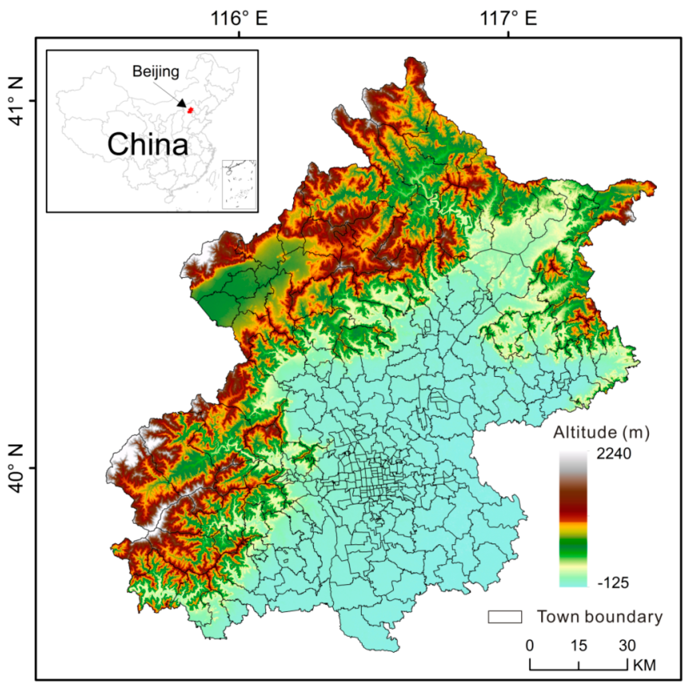
Beijing, the capital of China, is situated at the northern tip of the North China Plain (39°28′~41°05′N, 115°25′~117°30′E) and covers a total area of 16,410.54 km2. The western, northern and northeastern regions of Beijing City are mostly mountainous, with altitudes ranging from 1000 to 1500 m. The southeastern part is a plain with altitudes that range from 20 to 60 m. Beijing has 16 districts, which contain a total of 329 town-level administrative units. According to the sixth national census of China in 2010, the total population of Beijing is ~19.61 million. The spatial distribution of Beijing’s settlements is very uneven, with most of the population concentrated in the central urban areas and the center of suburban districts (see Figure 1).
2.2. Data
2.2.1. Population Data
Population data comes from the sixth census of China in 2010, which can be freely accessed at the National Bureau of Statistics of China. China conducts a national population census every 10 years. It is an extensive, one-time survey of the entire national population. Investigators visit each household to conduct surveys, which ensures the authenticity, accuracy, and completeness of the census data. In this study, the total resident population of the 329 town-level administrative units in Beijing City was derived from the 2010 census dataset.
2.2.2. Remote Sensing Data
In 2010, only DMSP/OLS provided night-time night remote sensing data. The NPP/VIIRS, which has better spatial resolution and data quality compared with DMSP/OLS was not available before April 2012. In view of the oversaturation problem of DMSP/OLS in urban areas, this study used NPP/VIIRS data from 2012 for population spatialization.
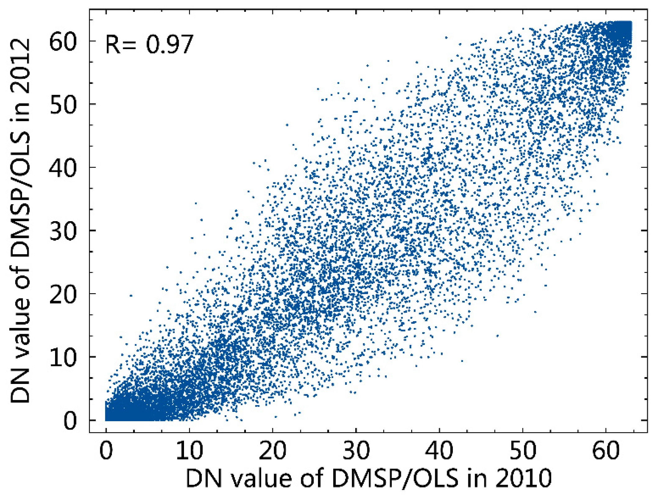
Considering the two-year difference between the census data and NPP/VIIRS data, the temporal difference in night-time lights in Beijing was analyzed first. The DMSP/OLS NTL data in 2010 and 2012 in Beijing were compared (Figure 2). The scatterplot suggested that there was a clear, positive correlation between them, with a high correlation coefficient of 0.97. By visual interpretation, the outliers in the scatterplot were mostly scenic spots, ecological reconstruction areas, industrial and mining areas, which generally have few residents. Therefore, by masking these regions, the NPP/VIIRS in 2012 can be used for mapping population in 2010.
The 500-m resolution monthly composite NPP/VIIRS NTL data [34] from April 2012 to December 2012 were used in this study. The annual NTL were calculated by averaging the monthly composite NPP/VIIRS NTL data. The mean NTL in forest and water bodies was calculated as the minimum NTL value to filter out background noise. In addition, the NTL values of the extremely lit areas at the Capital International Airport and the National Theatre were replaced by the mean NTL value of urban areas.
Landsat5/TM images on 26 July 2011 were used in this study for land cover classification and land surface temperature retrieval. Landsat5/TM data have seven bands, of which six multispectral bands have a spatial resolution of 30 m, and one thermal infrared band has a spatial resolution of 120 m.
The Advanced Spaceborne Thermal Emission and Reflection Radiometer Global Digital Elevation Map (ASTER/GDEM) data (Version 2) at a spatial resolution of 30 m was employed in this study to extract the elevation and slope of Beijing.
2.2.3. Vector Data
Road network data was derived from OpenStreetMap, an online open-source and editable map platform where all the contents are provided and maintained free of charge by the public. It provides valuable information for disaster relief, map data industry development, and geospatial scientific research. The road network derived for Beijing was cleaned to eliminate false data.
2.3. Method
This paper mapped the population density in Beijing based on the spatial variables derived from multi-source datasets. Firstly, 13 spatial variables were derived from NPP/VIIRS NTL, ASTER GDEM, Landsat/TM, OpenSreetMap road network and administrative district data, including night-time light (NTL), Built-up coverage (BC), water coverage (WC), forest coverage (FC), bare land coverage (BLC), industrial and mining coverage (IMC), grassland coverage (GC), cropland coverage (CC), land surface temperature (LST), altitude (ALT), flat area coverage (FAC), road network density (RND) and urban function type (UFT). Then, traditional linear regression and five machine learning algorithms were introduced for modeling at the town level: multiple linear regression (MLR), least absolute shrinkage and selection operator (LASSO), Bayesian regularized neural networks (BRNN), support vector machines with radial basis function kernel (SVM), random forest (RF) and extreme gradient boosting (XGBoost). These six predictive algorithms were compared in order to develop an optimal model with best performance. The final developed model was applied on the gridded spatial input variables to map population distribution in Beijing. Finally, the pixel values in the preliminary gridded population were adjusted by the census data so that the population of each town-unit was consistent with the town-level census population. A summary of the population spatialization found in this study is outlined below and also shown in Figure 3.
2.3.1. Independent Variables
To develop models for population estimation, a number of independent variables were derived from remote sensing data.
Night-time light, which can effectively reflect socio-economic activities [35,36,37,38,39], has a close relationship with population distribution. In this study, NTL was used as a socio-economic related feature for population modeling.
Studies show that agricultural land and water in Beijing have continued to shrink over the past two decades, and have generally been replaced by man-made, impervious surfaces. An important factor in this change is the rapid growth of the population [40]. Land cover directly reflects the human impact on the natural environment, and therefore was used as a feature to describe the land characteristics in population spatialization. Landsat5/TM data was used for land cover classification. In addition to Landsat5/TM multi-spectral bands, the normalized difference vegetation index (NDVI), the modified normalized difference water index (MNDWI), the GDEM elevation and spatial texture characteristics were also employed as classification features. Training and validation samples were visually selected from high-resolution images from Google Earth that contain eight land cover categories (built-up, industrial and mining, cropland, forest, grassland, bare land, water and cloud). The land cover map in Beijing was generated based on the Classification And Regression Tree (CART) decision tree algorithm (Figure 4) with an overall classification accuracy of 92.64%, and a Kappa coefficient of 0.91. The land cover types (BC, WC, FC, BLC, IMC, GC and CC) were used as the land cover indicators.
The urban thermal environment, which is highly impacted by manmade surfaces and anthropogenic heat, was used as an indicator of local climate for population spatialization. The daytime LST was derived from Landsat5/TM data to determine the urban thermal environment of Beijing. The land surface emissivity was calculated using a hybrid pixel method [41,42], and the atmospheric water vapor content was derived from the TERRA/MODIS water vapor product (MOD05) on Landsat5/TM imaging data. Finally, the daytime LST in Beijing (Figure 5) was retrieved based on the single-channel algorithm proposed by Jiménez-Muñoz et al. [43].
The western and northern parts of Beijing are mainly mountainous, whereas the south-east region is a vast plain. This topographical condition has an important impact on the population distribution of Beijing. The ALT and FAC (slope < 5°) were employed as terrain features of the population spatialization.
The distribution of the urban population is highly dependent on traffic. The density of road networks in residential-intensive areas is often greater. RND was calculated from the road network provided by OSM and used as the traffic feature in the population modeling.
To facilitate overall planning and coordination, Beijing has divided districts into four types: capital function core district, urban function expansion district, urban development new district, and ecological conservation development district. Different population control policies are adopted in different districts. Owing to the different population policies, the population distribution in Beijing is influenced by the different urban functions. According to the function of each district, UFT was used as a policy feature.
In total, 13 independent spatial variables were selected to model the population spatialization: NTL, BC, WC, FC, BLC, IMC, GC, CC, LST, ALT, FAC, RND and UFT.
2.3.2. Modeling Method
MLR is a statistical technology that is widely used to derive the relationship between two or more independent variables and one dependent variable by fitting a linear equation. LASSO is a regression method that performs both feature selection and regularization [44]. It shrinks the coefficients of the less important variables towards zero to improve the accuracy and interpretability of the model. BRNN is a neural network that is based on Bayesian regularization, which is a mathematical technique to convert nonlinear regressions into “well-posed” problems [45]. It uses the Nguyen and Widrow algorithm [46] to assign initial weights and the Gauss-Newton algorithm to perform the optimization. The trainbr function is implemented as the training algorithm. Compared with standard back-propagation networks, BRNN is more robust and resistant to overfitting. SVM generates separating hyperplanes to define decision boundaries for classification. Later SVM is expanded for regression, which uses the same principles as that for classification. SVM uses kernel functions to map data to a higher dimension space. Among different types of kernel functions, the radial basis function is commonly used for its advances in handling nonlinear problems and effectiveness [47,48]. RF is an ensemble learning algorithm that consists of a collection of decision trees and can be used for classification and regression [49]. It uses the bagging technique to randomly select bootstrap samples for training multiple decision trees based on the CART algorithm. In addition, RF also randomly selects feature subsets for training during the generation of trees. Each individual tree produces its own predicted output and the final outputs of the whole RF model are the average of the outputs of all the trees. XGBoost is an ensemble algorithm based on gradient boosted trees [50]. It follows the gradient boosting principle proposed by Friedman [51], which iteratively trains additional better trees on the residuals of the previous trees. On the basis of gradient boosting, XGBoost applies second order Taylor expansion to optimize the objective function and applies regularization techniques to reduce overfitting. All the employed algorithms were implemented in the R statistical software.
The averaged values of all the 13 spatial independent variables (NTL, BC, WC, FC, BLC, IMC, GC, CC, LST, ALT, FAC, RND and UFT) of each town-level administrative unit were calculated as the independent variables, and the population density of each town-level unit derived from the census data were used as the dependent variable to fit modes for population estimation. MLR, LASSO, BRNN and SVM can only use continuous numeric variables, so UFT was removed and the remaining 12 spatial independent variables were employed for modeling. For RF and XGBoost, all the 13 spatial independent variables were employed for modeling. The values of the spatial independent variables of all the 329 town-level units in Beijing were used as samples to model the population distribution of Beijing in 2010.
Ten-fold cross-validation was used to verify the estimation performance of the models. Model accuracy was evaluated using the mean absolute error (MAE) and the determination coefficient (R2), as follows:
where n is the number of town-level administrative units, Popi is the actual population density of town-level unit i, and Popi′ is the estimated population density of town-level unit i.
where is the mean of actual population density of all town-level units.
During cross validation, tunable models were tuned to develop optimized models. The parameter values that can achieve the lowest MAE were chosen to fit the models. MLR has no tuning parameters. The usual tuning parameter of LASSO is the fraction of full solution (fraction). The usual tuning parameters of BRNN include the number of neurons (neurons), maximum number of epochs to train (epochs), and the parameter that controls the behavior of the Gauss-Newton optimization algorithm (mu). The usual tuning parameters of SVM include sigma and cost (C). The usual tuning parameters of RF include the number of trees (ntree), number of variables randomly sampled as candidates at each split (mtry), minimum size of terminal nodes (nodesize) and maximum number of terminal nodes trees (maxnodes). The usual tuning parameters of XGBoost include the number of boosting iterations (nrounds), max tree depth (max_depth), minimum loss reduction (gamma), subsample ratio of the training instance (subsample ratio of the training instance), subsample ratio of columns (colsample_bytree), shrinkage (eta), and minimum sum of instance weight (min_child_weight). To reduce the computation, only the most important tuning parameters of the tunable models were tuned and the other tuning parameters were set as default. Table 1 lists the tuned parameters of the six models in this study.
2.3.3. Variable Selection
To reduce the tendency of overfitting and the model complexity, feature selection was performed to reduce the number of independent variables. The correlation between town-level population density and the 13 variables were analyzed using the Pearson correlation coefficient and distance correlation coefficient as the indicators.
Similarly, and can be derived.
To reduce the computation effort, the three independent variables most correlated with population density were kept, and the full combinatorial operation was performed on the remaining independent variables to produce 2n-3−1 variable combinations. Each variable combination, together with the three kept variables, constituted 2n-3−1 feature sets. Ten-fold cross-validation was used to validate the performance of each feature set. The minimum MAE and average MAE of feature sets with different variable numbers were recorded. The minimum MAE represents the minimum error that can be obtained by inputting n independent variables, and the average MAE represents the stable error obtained by inputting n independent variables. When both the minimum MAE and the average MAE are small, the number of independent variables is the optimal choice, and the variable combination that produces the minimum MAE is the optimal combination for population modeling.
2.3.4. Population Spatialization
The values of all the selected variables were calculated at a uniform spatial resolution of 500 m. Then the developed optimal model was applied to the independent variables to obtain a 500-m gridded population density map of Beijing. Considering that there are generally no permanent residents in the pixels for pure forest, cropland, water, and bare land, the estimated population density of Beijing was adjusted by setting the value of these non-population pixels to zero.
Due to the modeling errors and the uncertainty caused by the scale gap between remote sensing pixels and the town-level unit, there will be some differences between the estimated population and the census data for each town-level administrative unit. To ensure that the population of each town-level unit is consistent with the actual census data population, the pixel values of the estimated population density in Beijing City were revised according to the following equation:
where Pop_correctedi,j is the revised population density of the j-th pixel of the town-level unit i, Pop_estimatedi,j is the estimated population density of the j-th pixel of the town-level unit i, Popi,census is the actual population of the town-level unit i, and N is the number of pixels of the town-level unit i. Areai is the area of a pixel (0.25 km2).
3. Results
Table 2 shows the cross validated MAE and R2 of the six models (MLR, LASSO, BRNN, SVM, RF and XGboost). Different models had varied estimation accuracies, with the MAE ranging from 2165.70 to 3105.61 people/km2, and the R2 ranging from 0.77 to 0.85. Of the six models, RF achieved the lowest MAE of 2165.70 people/km2 and the highest R2 of 0.85, suggesting that it was the optimal model for population density estimation. It was also noted that MLR, the widely-used algorithm in population spatialization, produced the highest MAE of 3105.61 people/km2 and the lowest R2 of 0.77. The poor performance of the MLR algorithm indicated that it does not capture the complex relationships between the population and related independent variables in the study area.
The Pearson correlation coefficient and distance correlation coefficient for the population density and the 13 independent variables in each township are shown in Table 3. The scatterplots of the population density and independent variables are also provided in Figure 6. There are strong correlations between NTL, BC, RND, LST and population density. The Pearson correlation coefficients were 0.77, 0.89, 0.82 and 0.75 respectively, and the distance correlation coefficients were 0.84, 0.91, 0.87 and 0.81 respectively. These four variables demonstrated different degrees of impact on population density in low-density and high-density areas. The variation in independent variables in low-density areas had little impact on population density, but demonstrated obvious demographic differences in high-density areas. The correlation between ALT, FC, CC and population density was not very strong, with Pearson correlation coefficients of −0.37, −0.45 and −0.53 respectively, and distance correlation coefficients of 0.46, 0.50, and 0.61 respectively. WC, BLC, IMC, and GC showed obvious weak correlations with population density compared with other variables. However, from the scatterplots it can be seen that these variables still showed some non-linear relationships with population density. When the population density was greater than 3000, BLC had a negative correlation with population density. The IMC ratio had a positive correlation with population density when it was less than 6%, and a negative correlation with population density when it was greater than 6%. The distance correlation coefficients also showed certain correlations between BLC, IMC and population density. UFT was able to characterize the circular expansion of Beijing’s urbanized area, that is, population density decreases towards the suburbs. Beijing’s urban population is generally distributed in flat areas, and the population in mountain areas is mostly distributed in valleys. FAC was not significantly correlated with population density in Beijing.
The first three variables (NTL, RND and BC) with the strongest correlation with population density were reserved, and all combinations for the 10 remaining variables (WC, FC, BLC, IMC, GC, CC, LST, ALT, FAC and UFT) were generated, which were 210−1 combinations. The fixed three variables and each of the combinations of the remaining 10 variables were combined to fit the model, which yielded a total set of 210−1 feature sets. The number of features range from four to 13 in all these 210−1 feature sets. When the number of features is four, it means that one variable was selected from the remaining 10 variables () and then combined with the fixed three variables, resulting in 10 different feature sets. When the number of features is five, it means that two variables were selected from the remaining 10 variables () and then combined with the fixed three variables, resulting in 45 different feature sets, and so on. When the number of features is 13, it means that all the remaining 10 variables were selected () and combined with the fixed three variables, resulting in only 1 feature sets. The accuracy of each feature set was validated using 10-fold cross-validation. Based on the cross-validated MAE of all the feature sets, the minimum MAE and average MAE with various numbers of independent variables were calculated and shown in Figure 7. The average MAE rapidly decreased as the number of variables increased from four to six and then slowly decreased with the increase of the number of variables. This suggested that when the number of variables was greater than six, the average error of the model tended to be stable. The minimum MAE (2129.52 people/km2) appeared when the number of variables was seven. Therefore, seven is the optimal number of variables for population modeling, and the seven variables that achieved the minimum error (NTL, RND, ALT, BC, CC, IMC, and LST) were employed for population modeling.
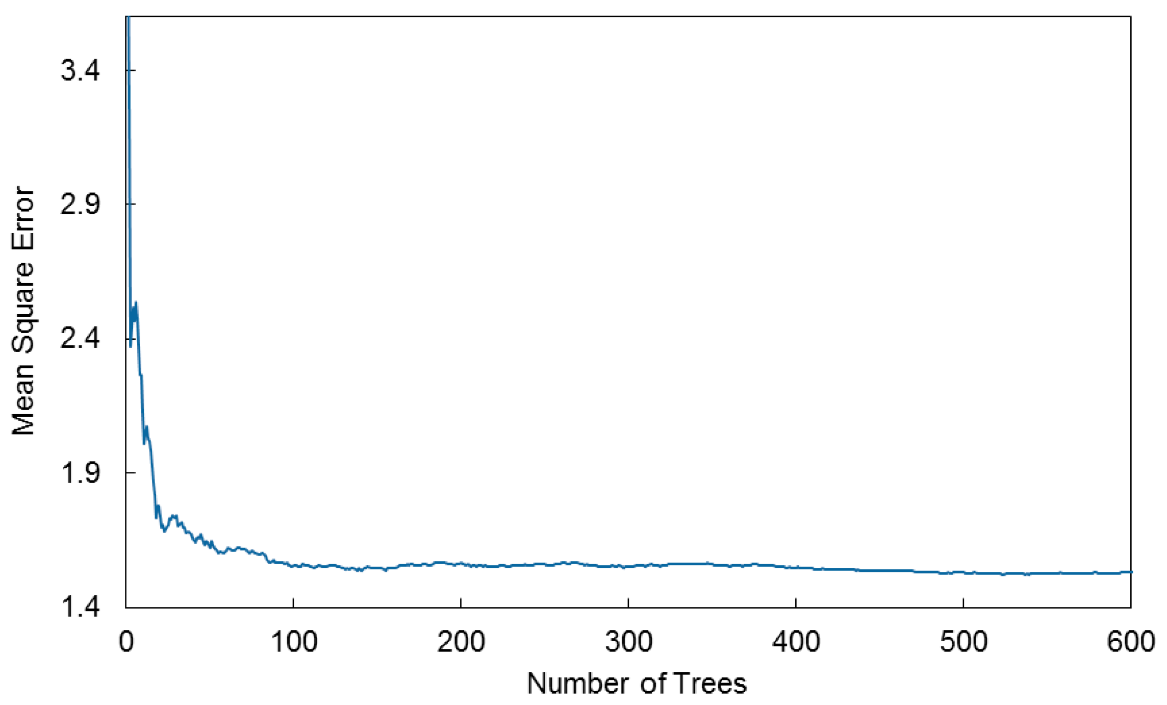
The selected seven input variables were used to fit the RF model. The parameter ntree was also tuned to optimize model performance (Figure 8), and the other three parameters (mtry, nodesize and maxnodes) were set as default. The mean square error decreased sharply when ntree increased to 30. When ntree increased from 30 to 100, the error decreased slowly and then flattened gradually. When ntree was greater than 400, the error was nearly unchanged. Therefore, ntree was set to 400 to fit the random forest model.
Figure 9 shows the scatterplot for the predicted population density from the random forest model and the actual population density from the census data at the town level. The random forest model achieved a cross-validated MAE of 2129.52 people/km2 and a cross-validated R2 of 0.63. Most of the samples were close to the 1:1 line, suggesting a good fitting performance.
The developed random forest model was applied to the 500 m resolution gridded variables (NTL, RND, ALT, UC, CC, IMC, and LST) to generate a population density map of Beijing. The population density values of the pure pixels of forest, cropland, water and bare land were masked as zero. Considering that there were still some errors in the random forest model and applying the model developed at the town level on the gridded independent variables can cause some uncertainties, the remaining pixel values were also adjusted based on Equation (5) to be consistent with the census data at the town level. Finally, the 500 m gridded population density map of Beijing was developed (Figure 10).
4. Discussion
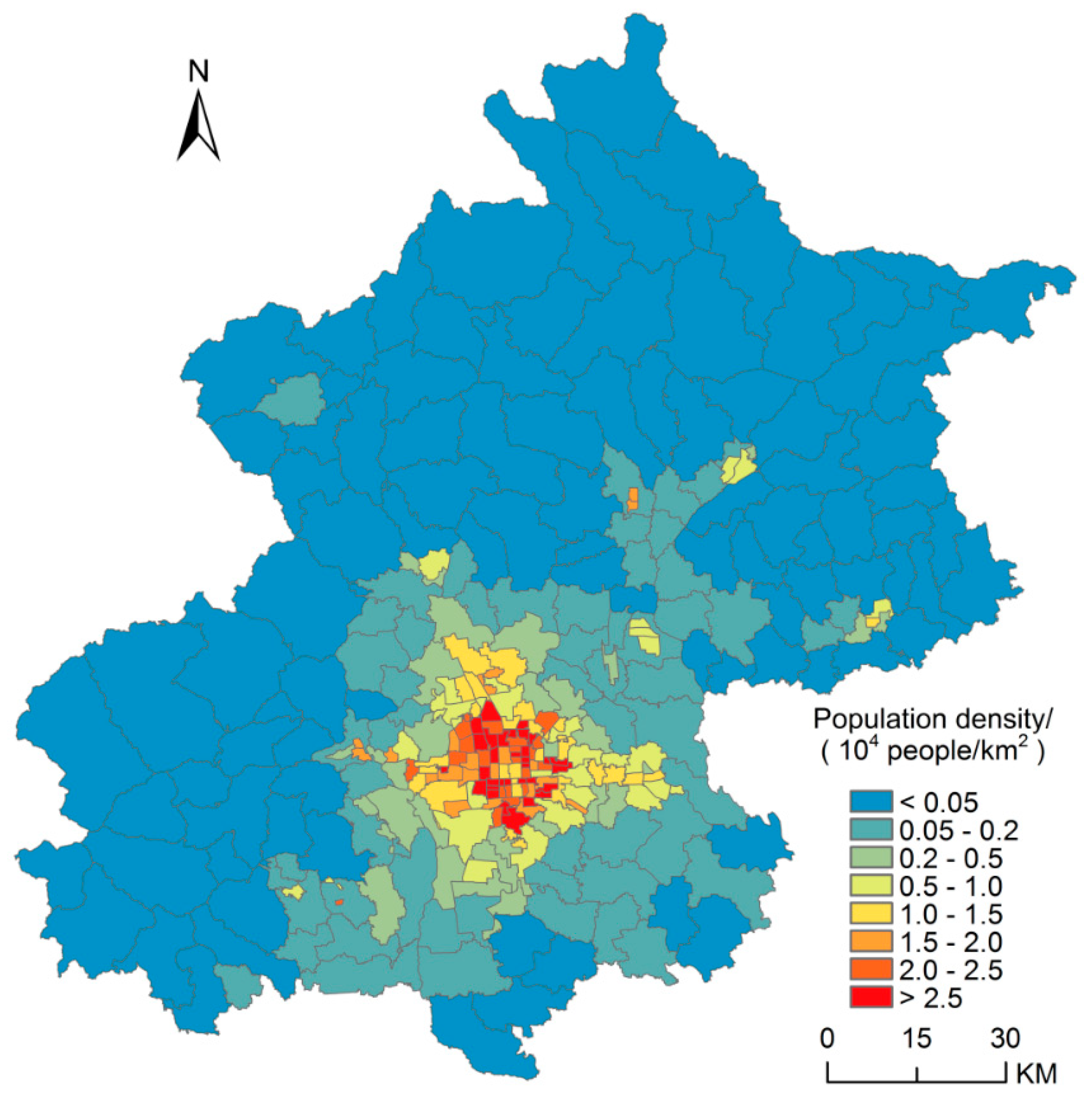
Compared with population census data at the town level, remotely-sensed population data gives the population density of each pixel and well depicts the spatial distribution of the population with greater detail. Figure 10 and Figure 11 show the population density maps derived from remotely sensed data and census data for Beijing, respectively. Generally, both the maps reflect the overall population distribution pattern in Beijing: the population is mainly concentrated in the urban districts, and the population density in suburb areas is generally low. However, the census data can only give the average population density of the town-level administrative units and cannot reflect the spatial differences within the town-level units. The remotely-sensed population redistributes the census population data to the 500 m pixels, which provides a lot more detailed spatial information than the census population data.
Due to the lack of population data for lower-level administrative units, the reliability of the remotely-sensed population data within town-level units cannot be quantitatively assessed. We selected three typical areas to discuss the rationality of remotely-sensed population distribution at the intra-town scale, using the high-resolution Google Earth images as a reference. The three selected areas were the North Taipingzhuang subdistrict in the main urban area, Yanqing town in the suburbs, and Changshaoying Manchu township in the mountains.
North Taipingzhuang subdistrict has a very high population density of 38,986.88 people/km2, and a very small area of 5.17 km2. From the Google Earth image (Figure 12a), it can be seen that this area was full of buildings. Especially in the southeast part, there are a lot of high residential buildings, which results in a higher population density than other parts. The remotely-sensed population density (Figure 12c) well reflects this spatial pattern, while the census data (Figure 12b) only provides a high average population density for this region.
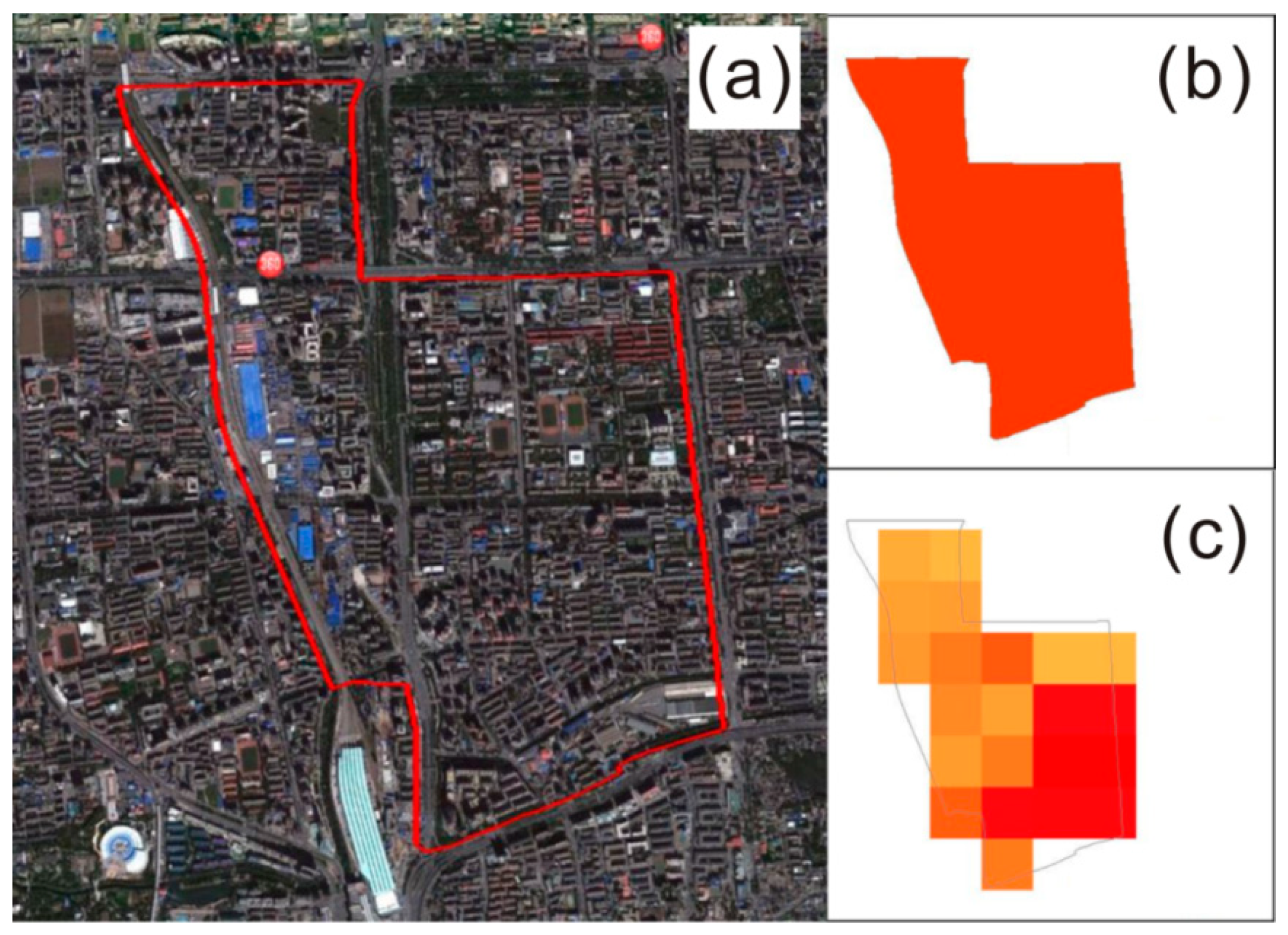
The spatial distribution of the population in the suburbs is generally much lower and more uneven than that in urban areas. Yanqing, a suburb town located in the northwest part of Beijing, has a medium population density of 1794.23 persons/km2, and a total area of 75 km2. From the Google Earth image (Figure 13a), it can be seen that the town center area in the southeast is dominated by multi-storied residential buildings, while the residential areas outside the town center are characterized by bungalows. Except for residential areas, there are mainly croplands that have no residents. The remotely-sensed result (Figure 13c) also well reflected the spatial distribution of the population, which is higher in the town center and surrounding areas. The census data (Figure 13b) cannot reflect this spatial difference in the town.
The Changshaoying Manchu township, is located in the northern mountains of Beijing, and covers a large area of 249.44 km2, but it has a very low population density of 26.37 people/km2. The Google Earth high-resolution remote sensing image (Figure 14a) showed that this region is mainly mountainous woodlands, with very few residential areas scattered across several valleys. In the remotely-sensed population map (Figure 14c), only a few pixels had relatively low population densities, and most pixels had a population density of zero. The spatial pattern of the remotely-sensed population density was well consistent with the Google Earth image. The census data (Figure 14b) gave a very low average population density for the whole township, which does not reflect the populated areas in the valleys.
Previous studies on population spatialization have generally been conducted at the county or higher level. Models were developed based on county-level administrative units and then applied to gridded independent variables to redistribute population from irregular administrative units to regular grids. The relatively large spatial gap between the county-unit and remote sensing pixel will introduce some uncertainties into the result [53]. However, it is difficult to measure the uncertainties caused by this spatial gap. To reduce the influence of the spatial gap, population spatialization should be performed at lower administrative levels. In this paper, we mapped the population density in Beijing at the town scale. Compared with county-level administrative districts, town-level districts have a much smaller area, which can effectively reduce the spatial gap between remote sensing data and census data. Due to the lack of detailed population data, the accuracy of remotely-sensed population data at the intra-town scale cannot be quantitatively assessed. To our knowledge, no previous studies have been carried out to validate the accuracy of gridded population datasets within census units. As an alternative, we used high-resolution Google Earth images as a reference to qualitatively validate the result. According to the results for three typical regions, the remotely-sensed population can well describe the detailed spatial distribution of the population within town-level units.
NTL data effectively depicts the spatial distribution of human activities at night and is widely used for population spatialization. However, considering the complexity of population, social, economic and natural conditions, taking NTL as the only independent variable cannot accurately reflect the population distribution, especially at fine spatial scales. In recent years, machine learning technology has been introduced for population spatialization based on NTL and other spatial variables [31,33,54,55]. However, most of the studies only used the RF algorithm for population modeling. Even though RF has been widely used in remote sensing applications, there are still a lot of other machine learning methods, such as artificial network, SVM, generalized linear models and other ensemble learning algorithms. This study employed several typical machine learning algorithms and compared their modeling performance by cross validation. Results showed that RF outperformed other methods and it had the lowest MAE and highest R2, suggesting that it is the optimal method to develop the population spatialization model. In addition, considering that using a lot of independent variables will produce complicated models, feature selection was conducted to reduce the risk of overfitting and the model complexity. The good results suggest that the proposed method can well fit the relationship between population density and spatial variables, and also produce a reliable spatial distribution of population.
Due to the lack of population census data at lower administrative levels, the remotely-sensed population found in this study was not quantitatively assessed at the intra-town level. In 2020, China will conduct the seventh national population census, which may provide more detailed population data. Therefore, more comprehensive work on population spatialization and evaluation can be carried out based on the new census data.
5. Conclusions
In this study, we mapped the population density in Beijing at the town scale based on random forest and multisource remote sensing data. Thirteen spatial independent variables (NTL, Alt, BC, WC, FC, BLC, IMC, GC, CC, UFT, FAC, RND, and LST) were derived from NPP/VIIRS and other remote sensing data. The comparison between the MLR and five machine learning algorithms indicated that RF achieved the best accuracy and was selected for population spatialization. By feature selection, seven variables (NTL, RND, ALT, BC, CC, IMC, and LST) were selected to fit the random forest model, which achieved a cross-validated MAE of 2129.52 people/km2 and a R2 of 0.63. The 500 m gridded population in Beijing was produced by applying the developed random forest model to gridded independent variables. Moreover, the produced gridded population was adjusted to be consistent with the census data at the town scale. The finally developed gridded population density well depicts the detailed spatial distribution of the population of Beijing, and shows much higher spatial heterogeneity than the census data.
Compared with other studies, this study comprehensively compared several machine learning algorithms to develop an optimal spatialization model to map population from multiple spatial variables at the town level. In addition, a qualitative assessment using Google Earth images as references was proposed to validate the reliability of the gridded population density results at the intra-town scale. The assessment result indicated that the developed gridded population reasonably reflects the population distribution information within town-level units. All the datasets employed in this study can be free accessed, and the machine learning algorithms can be implemented in R or Python. The details of the data processing, modeling and validation are described in this paper. Therefore, the method proposed in this study could serve as a good template for population spatialization in other cities. The results of this study provide a valuable reference for various applications with regard to Beijing. For urban planning, the gridded population data provides detailed information about the population distribution for municipal infrastructure construction, road network design, and the distribution of schools, hospitals and parks. For natural disaster prevention and control, gridded population data is helpful to accurately assess the exposed population and effective emergency response in disasters. The detailed population distribution can also be incorporated in accessibility modeling, commercial site selection and infectious disease research.
Author Contributions
Conceptualization, Y.X; methodology, Y.X. and M.H.; formal analysis, M.H. and N.L.; investigation, M.H. and N.L.; writing—original draft preparation, M.H.; writing—review and editing, M.H., Y.X. and N.L.; supervision, Y.X.; project administration, Y.X. All authors have read and agreed to the published version of the manuscript.
Funding
This research was funded by the Humanities and Social Sciences Foundation of the Ministry of Education of China (grant number 17YJCZH205), the Environmental Monitoring Foundation of Jiangsu Province (grant number 1903) and Qing Lan Project of Jiangsu Province (grant number R2019Q03).
Acknowledgments
The authors would like to thank the National Bureau of Statistics of China for providing census data, NOAA Earth Observation Group (EOG) for providing NPP/VIIRS night-time data, US Geological Survey (USGS) for providing SRTM/DEM data, United States Geological Survey for providing Landsat data, and the Earth Remote Sensing Data Analysis Center of Japan for providing ASTER/GDEM data, and Open Street Map for providing geographic information data.
Conflicts of Interest
The authors declare no conflict of interest.
References
- United Nations, Department of Economic and Social Affairs, Population Division. World Urbanization Prospects: The 2018 Revision; United Nations: New York, NY, USA, 2019; pp. 1–8. [Google Scholar]
- Liang, W.; Yang, M. Urbanization, economic growth and environmental pollution: Evidence from China. Sustain. Comput. Inform. 2019, 21, 1–9. [Google Scholar] [CrossRef]
- Aghion, P.; Durlauf, S. (Eds.) Handbook of Economic Growth; Elsevier: Amsterdam, The Netherlands, 2005; pp. 1559–1560. [Google Scholar]
- Ameen, R.F.M.; Mourshed, M. Urban environmental challenges in developing countries—A stakeholder perspective. Habitat Int. 2017, 64, 1–10. [Google Scholar] [CrossRef]
- Palanivel, T. Rapid Urbanisation: Opportunities and Challenges to Improve the Well-Being of Societies; United Nation Development Programme: New York, NY, USA, 2017. [Google Scholar]
- Mesev, V. Remotely-Sensed Cities; CRC Press: Boca Raton, FL, USA, 2003; pp. 1–19. [Google Scholar]
- Talukdar, K.K. Tele-Geoinformation Service for Sustainable Urban Management: A Satellite-based Observation Approach for the 21st Century. In Proceedings of the International Symposium, Strasbourg, France, 3–5 June 1998; pp. 149–155. [Google Scholar]
- Mesev, V. Classification of Urban Areas: Inferring Land Use from the Interpretation of Land Cover. In Remote Sensing of Urban and Suburban Areas; Rashed, T., Jürgens, C., Eds.; Springer: Strasbourg, France, 2010; pp. 141–164. [Google Scholar]
- Zhu, Z.; Zhou, Y.; Seto, K.C.; Stokes, E.C.; Deng, C.; Pickett, S.T.; Taubenböck, H. Understanding an urbanizing planet: Strategic directions for remote sensing. Remote Sens. Environ. 2019, 228, 164–182. [Google Scholar] [CrossRef]
- Maktav, D.; Erbek, F.S.; Jürgens, C. Remote sensing of urban areas. Int. J. Remote Sens. 2005, 26, 655–659. [Google Scholar] [CrossRef]
- Balk, D.L.; Deichmann, U.; Yetman, G.; Pozzi, F.; Hay, S.I.; Nelson, A. Determining global population distribution: Methods, applications and data. Adv. Parasitol. 2006, 62, 119–156. [Google Scholar]
- Linard, C.; Alegana, V.A.; Noor, A.M.; Snow, R.W.; Tatem, A.J. A high resolution spatial population database of Somalia for disease risk mapping. Int. J. Health Geogr. 2010, 9, 1–13. [Google Scholar] [CrossRef] [PubMed]
- Gaughan, A.E.; Stevens, F.R.; Linard, C.; Jia, P.; Tatem, A.J. High resolution population distribution maps for Southeast Asia in 2010 and 2015. PLoS ONE 2013, 8, e55882. [Google Scholar] [CrossRef] [PubMed]
- Langford, M.; Higgs, G.; Radcliffe, J.; White, S. Urban population distribution models and service accessibility estimation. Comput. Environ. Urban Syst. 2008, 32, 66–80. [Google Scholar] [CrossRef]
- Silvan-Cardenas, J.L.; Wang, L.; Rogerson, P.; Wu, C.; Feng, T.; Kamphaus, B.D. Assessing fine-spatial-resolution remote sensing for small-area population estimation. Int. J. Remote Sens. 2010, 31, 5605–5634. [Google Scholar] [CrossRef]
- Calka, B.; Nowak Da Costa, J.; Bielecka, E. Fine scale population density data and its application in risk assessment. Geomat. Nat. Hazards Risk 2017, 8, 1440–1455. [Google Scholar] [CrossRef]
- Clark, C. Urban Population Densities. J. R. Stat. Soc. 1951, 114, 490–496. [Google Scholar] [CrossRef]
- Martin, D. Mapping Population Data from Zone Centroid Locations. Trans. Inst. Br. Geogr. 1989, 14, 90–97. [Google Scholar] [CrossRef] [PubMed]
- Gallego, F.J. A population density grid of the European Union. Popul. Environ. 2010, 31, 460–473. [Google Scholar] [CrossRef]
- Lo, C.P. Population Estimation Using Geographically Weighted Regression. GISci. Remote Sens. 2008, 45, 131–148. [Google Scholar] [CrossRef]
- Lung, T.; Lübker, T.; Ngochoch, J.K.; Schaab, G. Human population distribution modelling at regional level using very high resolution satellite imagery. Appl. Geogr. 2013, 41, 36–45. [Google Scholar] [CrossRef]
- Sutton, P. Modeling population density with night-time satellite imagery and GIS. Comput. Environ. Urban Syst. 1997, 21, 227–244. [Google Scholar] [CrossRef]
- Briggs, D.J.; Gulliver, J.; Fecht, D.; Vienneau, D.M. Dasymetric modelling of small-area population distribution using land cover and light emissions data. Remote Sens. Environ. 2007, 108, 451–466. [Google Scholar] [CrossRef]
- Bagan, H.; Yamagata, Y. Analysis of urban growth and estimating population density using satellite images of nighttime lights and land-use and population data. GISci. Remote Sens. 2015, 52, 765–780. [Google Scholar] [CrossRef]
- Amaral, S.; Monteiro, A.M.V.; Camara, G.; Quintanilha, J.A. DMSP/OLS night-time light imagery for urban population estimates in the Brazilian Amazon. Int. J. Remote Sens. 2006, 27, 855–870. [Google Scholar] [CrossRef]
- Sun, W.; Zhang, X.; Wang, N.; Cen, Y. Estimating Population Density Using DMSP-OLS Night-Time Imagery and Land Cover Data. IEEE J. Sel. Top. Appl. Earth Obs. Remote Sens. 2017, 10, 2674–2684. [Google Scholar] [CrossRef]
- Elvidge, C.D.; Cinzano, P.; Pettit, D.R.; Arvesen, J.; Sutton, P.; Small, C.; Nemani, R.; Longcore, T.; Rich, C.; Safran, J.; et al. The Nightsat mission concept. Int. J. Remote Sens. 2007, 28, 2645–2670. [Google Scholar] [CrossRef]
- Cao, C.; De Luccia, F.; Xiong, X.; Wolfe, R.; Weng, F. Early on-orbit performance of the Visible Infrared Imaging Radiometer Suite (VIIRS) onboard the Suomi National Polar-orbiting Partnership (S-NPP) satellite. IEEE Trans. Geosci. Remote Sens. 2014, 52, 1142–1156. [Google Scholar] [CrossRef] [Green Version]
- Liao, L.B.; Weiss, S.; Mills, S.; Hauss, B. Suomi NPP VIIRS day-night band on-orbit performance. J. Geophys. Res. Atmos. 2013, 118, 718. [Google Scholar] [CrossRef]
- Chen, X.; Nordhaus, W. A Test of the New VIIRS Lights Data Set: Population and Economic Output in Africa. Remote Sens. 2015, 7, 4937–4947. [Google Scholar] [CrossRef] [Green Version]
- Stevens, F.R.; Gaughan, A.E.; Linard, C.; Tatem, A.J. Disaggregating Census Data for Population Mapping Using Random Forests with Remotely-Sensed and Ancillary Data. PLoS ONE 2015, 10, e0107042. [Google Scholar] [CrossRef] [PubMed] [Green Version]
- Chen, J.; Fan, W.; Li, K.; Liu, X.; Song, M. Fitting Chinese cities’ population distributions using remote sensing satellite data. Ecol. Indic. 2019, 98, 327–333. [Google Scholar] [CrossRef]
- Gaughan, A.E.; Stevens, F.R.; Linard, C.; Patel, N.; Tatem, A.J. Exploring nationally and regionally defined models for large area population mapping. Int. J. Digit. Earth 2015, 8, 989–1006. [Google Scholar] [CrossRef]
- Baugh, K.; Hsu, F.C.; Elvidge, C.D.; Zhizhin, M. Nighttime lights compositing using the VIIRS day-night band: Preliminary results. Proc. Asia Pac. Adv. Netw. 2013, 35, 70–86. [Google Scholar] [CrossRef] [Green Version]
- Small, C.; Pozzi, F.; Elvidge, C.D. Spatial analysis of global urban extent from DMSP-OLS night lights. Remote Sens. Environ. 2005, 96, 277–291. [Google Scholar] [CrossRef]
- Wen, W.; Hui, C.; Zhang, L.I. Poverty assessment using DMSP/OLS night-time light satellite imagery at a provincial scale in China. Adv. Space Res. 2012, 49, 1253–1264. [Google Scholar]
- Shi, K.; Chen, Y.; Yu, B.; Xu, T.; Yang, C.; Li, L.; Huang, C.; Chen, Z.; Liu, R.; Wu, J. Detecting spatiotemporal dynamics of global electric power consumption using DMSP-OLS nighttime stable light data. Appl. Energy 2016, 184, 450–463. [Google Scholar] [CrossRef]
- Zhao, M.; Cheng, W.; Zhou, C.; Li, M.; Wang, N.; Liu, Q. GDP Spatialization and Economic Differences in South China Based on NPP-VIIRS Nighttime Light Imagery. Remote Sens. 2017, 9, 673. [Google Scholar] [CrossRef] [Green Version]
- Bennett, M.M.; Smith, L.C. Advances in using multitemporal night-time lights satellite imagery to detect, estimate, and monitor socioeconomic dynamics. Remote Sens. Environ. 2017, 192, 176–197. [Google Scholar] [CrossRef]
- Xiao, Y.; Wang, Y.H.; Yin, C.H. Driving Force Analysis of Land Use Chang of Beijing Urban Areas in the Past 20 Years. Geomat. Spat. Inf. Technol. 2013, 36, 29–32. (In Chinese) [Google Scholar]
- Sobrino, J.A.; Jiménez-Muñoz, J.C.; Paolini, L. Land surface temperature retrieval from Landsat TM5. Remote Sens. Environ. 2004, 90, 434–446. [Google Scholar] [CrossRef]
- Qin, Z.; Li, W.; Gao, M.; Zhang, H. Estimation of land surface emissivity for Landsat TM6 and its application to Lingxian region in North China. In Proceedings of the Remote Sensing for Environmental Monitoring, GIS Applications, and Geology VI, Stockholm, Sweden, 3 October 2006; p. 636618. [Google Scholar]
- Jiménez-Muñoz, J.C.; Cristóbal, J.; Sobrino, J.A.; Sòria, G.; Ninyerola, M.; Pons, X. Revision of the single-channel algorithm for land surface temperature retrieval from Landsat thermal-infrared data. IEEE Trans. Geosci. Remote Sens. 2009, 47, 339–349. [Google Scholar] [CrossRef]
- Tibshirani, R. Regression shrinkage and selection via the lasso. J. R. Stat. Soc. Ser. B Stat. Methodol. 1996, 58, 267–288. [Google Scholar] [CrossRef]
- Burden, F.; Winkler, D. Bayesian regularization of neural networks. Methods Mol. Biol. 2008, 458, 25–44. [Google Scholar]
- Nguyen, D.; Widrow, B. Improving the learning speed of 2-layer neural networks by choosing initial values of the adaptive weights. In Proceedings of the International Joint Conference of Neural Networks, San Diego, CA, USA, 17–21 June 1990; pp. 21–26. [Google Scholar]
- Bennett, K.P.; Campbell, C. Support vector machines: Hype or hallelujah? SIGKDD Explor. 2000, 2, 1–13. [Google Scholar] [CrossRef]
- Hsu, C.; Chang, C.; Lin, C. A practical guide to support vector classification. BJU Int. 2008, 101, 1396–1400. [Google Scholar]
- Breiman, L. Random forests. Mach. Learn. 2001, 45, 5–32. [Google Scholar] [CrossRef] [Green Version]
- Chen, T.; Guestrin, C. XGBoost: A scalable tree boosting system. In Proceedings of the 22nd ACM SIGKDD International Conference on Knowledge Discovery and Data Mining, San Francisco, CA, USA, 13–17 August 2016; pp. 785–789. [Google Scholar]
- Friedman, J.H. Greedy function approximation: A gradient boosting machine. Ann. Stat. 2001, 29, 1189–1232. [Google Scholar] [CrossRef]
- Székely, G.J.; Rizzo, M.L.; Bakirov, N.K. Measuring and Testing Dependence by Correlation of Distances. Ann. Stat. 2008, 35, 2769–2794. [Google Scholar] [CrossRef]
- Liang, H.; Guo, Z.; Wu, J.; Chen, Z. GDP spatialization in Ningbo City based on NPP/VIIRS night-time light and auxiliary data using random forest regression. Adv. Space Res. 2020, 65, 481–493. [Google Scholar] [CrossRef]
- Yao, Y.; Liu, X.; Li, X.; Zhang, J.; Liang, Z.; Mai, K.; Zhang, Y. Mapping fine-scale population distributions at the building level by integrating multi-source geospatial big data. Int. J. Geogr. Inf. Sci. 2017, 31, 1220–1244. [Google Scholar]
- Ye, T.; Zhao, N.; Yang, X.; Ouyang, Z.; Liu, X.; Chen, Q.; Hu, K.; Yue, W.; Qi, J.; Li, Z.; et al. Improved population mapping for China using remotely sensed and points-of-interest data within a random forests model. Sci. Total Environ. 2019, 658, 936–946. [Google Scholar] [CrossRef] [PubMed]
Figure 1.
Location and administrative divisions of Beijing.

Figure 2.
Scatter plot between the DN values of Defense Meteorological Satellite Program/ Operational Line Scanner DMSP/OLS Night-time light (NTL) in 2010 and 2012 in Beijing.
Figure 2.
Scatter plot between the DN values of Defense Meteorological Satellite Program/ Operational Line Scanner DMSP/OLS Night-time light (NTL) in 2010 and 2012 in Beijing.

Figure 3.
Flowchart of population spatialization in Beijing.

Figure 4.
Land cover map in Beijing.

Figure 5.
Daytime land surface temperature in Beijing.

Figure 6.
Scatterplot of township population density and 13 independent variables (a–m).

Figure 7.
Variations of the minimum and average mean absolute error (MAE) with the number of variables.
Figure 7.
Variations of the minimum and average mean absolute error (MAE) with the number of variables.

Figure 8.
Relationship between the number of decision trees and the mean square error.

Figure 9.
Scatterplot for the estimated population density from the random forest model and the actual population density from census data.
Figure 9.
Scatterplot for the estimated population density from the random forest model and the actual population density from census data.

Figure 10.
Remotely-sensed population density map of Beijing.

Figure 11.
Population density map of Beijing derived from census data.

Figure 12.
Comparison of the Google Earth image (a), census population data (b) and remotely-sensed population (c) in North Taipingzhuang subdistrict. The red line in (a) is the boundary of the subdistrict. Figures b and c use the same legend as Figure 9.
Figure 12.
Comparison of the Google Earth image (a), census population data (b) and remotely-sensed population (c) in North Taipingzhuang subdistrict. The red line in (a) is the boundary of the subdistrict. Figures b and c use the same legend as Figure 9.

Figure 13.
Comparison of the Google Earth image (a), census population data (b) and remotely-sensed population (c) in Yanqing Town. The red line in (a) is the boundary of the town. Figures b and c use the same legend as Figure 9.
Figure 13.
Comparison of the Google Earth image (a), census population data (b) and remotely-sensed population (c) in Yanqing Town. The red line in (a) is the boundary of the town. Figures b and c use the same legend as Figure 9.

Figure 14.
Comparison of the Google Earth image (a), census population data (b) and remotely-sensed population data (c) in Changshaoying Manchu township. The red line in (a) is the boundary of the township. Figures b and c use the same legend as Figure 9.
Figure 14.
Comparison of the Google Earth image (a), census population data (b) and remotely-sensed population data (c) in Changshaoying Manchu township. The red line in (a) is the boundary of the township. Figures b and c use the same legend as Figure 9.


Table 1.
Tuned parameters for the six models in this study.
| Model | Tuned Parameter |
|---|---|
| MLR | / |
| LASSO | fraction |
| BRNN | neurons |
| SVMR | Sigma, C |
| RF | ntree |
| XGBoost | nrounds, max_depth, gamma, subsample, colsample_bytree |
Table 2.
Accuracy of population density estimation of the six models.
| Model | MAE (People/km2) | R2 |
|---|---|---|
| MLR | 3105.61 | 0.77 |
| LASSO | 3072.15 | 0.77 |
| BRNN | 2379.93 | 0.80 |
| SVMR | 2520.11 | 0.82 |
| RF | 2165.70 | 0.85 |
| XGBoost | 2456.50 | 0.83 |
Table 3.
Correlation coefficients between independent variables and population density.
| Variable | Pearson Correlation Coefficient | Distance Correlation Coefficient |
|---|---|---|
| NTL | 0.77 | 0.84 |
| ALT | −0.37 | 0.46 |
| BC | 0.89 | 0.91 |
| WC | −0.13 | 0.18 |
| FC | −0.45 | 0.50 |
| BLC | −0.28 | 0.39 |
| IMC | 0.24 | 0.49 |
| GC | 0.15 | 0.37 |
| CC | −0.53 | 0.61 |
| UFT | −0.64 | 0.68 |
| FAC | −0.24 | 0.27 |
| RND | 0.82 | 0.87 |
| LST | 0.75 | 0.81 |
© 2020 by the authors. Licensee MDPI, Basel, Switzerland. This article is an open access article distributed under the terms and conditions of the Creative Commons Attribution (CC BY) license (http://creativecommons.org/licenses/by/4.0/).
Share and Cite
MDPI and ACS Style
He, M.; Xu, Y.; Li, N. Population Spatialization in Beijing City Based on Machine Learning and Multisource Remote Sensing Data. Remote Sens. 2020, 12, 1910. https://0-doi-org.brum.beds.ac.uk/10.3390/rs12121910
AMA Style
He M, Xu Y, Li N. Population Spatialization in Beijing City Based on Machine Learning and Multisource Remote Sensing Data. Remote Sensing. 2020; 12(12):1910. https://0-doi-org.brum.beds.ac.uk/10.3390/rs12121910
Chicago/Turabian StyleHe, Miao, Yongming Xu, and Ning Li. 2020. "Population Spatialization in Beijing City Based on Machine Learning and Multisource Remote Sensing Data" Remote Sensing 12, no. 12: 1910. https://0-doi-org.brum.beds.ac.uk/10.3390/rs12121910
Note that from the first issue of 2016, this journal uses article numbers instead of page numbers. See further details here.