Uncertainty in Satellite-Derived Surface Irradiances and Challenges in Producing Surface Radiation Budget Climate Data Record

 ,
,  ,
,
Abstract
:
1. Introduction
2. Uncertainty Estimate
2.1. Uncertainty in the Net Surface and Atmospheric Irradiances
2.2. Uncertainty in Surface Irradiance Trend and in Observing Decadal Surface Irradiance Change
3. Impact of New Generation Geostationary Satellites on Compute Surface Irradiances
4. Consistency Check Using Energy Balance
5. Discussion and Conclusions
Author Contributions
Funding
Acknowledgments
Conflicts of Interest
Appendix A

Appendix B


References
- Johnson, G.C.; Lyman, J.M.; Loeb, N.G. Loeb, Improving estimates of Earth’s energy imbalance. Nat. Clim. Chang. 2016, 6, 639–640. [Google Scholar] [CrossRef]
- Loeb, N.G.; Doelling, D.R.; Wang, H.; Su, W.; Nguyen, C.; Corbett, J.G.; Liang, L.; Mitrescu, C.; Rose, F.G.; Kato, S. Clouds and the Earth’s Radiant Energy System (CERES) Energy Balanced and Filled (EBAF) top-of-atmosphere (TOA) Edition-4.0 data product. J. Clim. 2018, 31, 895–918. [Google Scholar] [CrossRef]
- Su, W.; Corbett, J.; Eitzen, Z.; Liang, L. Next-generation angular distribution models for top-of-atmosphere radiative flux calculation from CERES instruments: Validation. Atmos. Meas. Tech. 2015, 8. [Google Scholar] [CrossRef] [Green Version]
- Loeb, N.G.; Wielicki, B.A.; Doelling, D.R.; Smith, G.L.; Keyes, D.F.; Kato, S.; Manalo-Smith, N.; Wong, T. Toward optimal closure of the Earth’s top-of-atmosphere radiation budget. J. Clim. 2009, 22, 748–766. [Google Scholar] [CrossRef] [Green Version]
- Rutan, D.A.; Kato, S.; Doelling, D.R.; Rose, F.G.; Nguyen, L.T.; Caldwell, T.E.; Loeb, N.G. CERES synoptic product: Methodology and validation of surface radiant flux. J. Atmos. Ocean. Technol. 2015, 32, 1121–1143. [Google Scholar] [CrossRef]
- Kato, S.; Rose, F.G.; Rutan, D.A.; Thorsen, T.J.; Loeb, N.G.; Doelling, D.R.; Huang, X.; Smith, W.L.; Su, W.; Ham, S.-H. Surface irradiances of Edition 4.0 Clouds and the Earth’s Radiant Energy System (CERES) Energy Balanced and Filled (EBAF) data product. J. Clim. 2018, 31. [Google Scholar] [CrossRef]
- Ohmura, A.; Dutton, E.; Forgan, B.; Frohlich, C.; Gilgen, H.; Hegne, H.; Heimo, A.; Konig-Langlo, G.; McArthur, B.; Muller, G.; et al. Baseline Surface Radiation Network (BSRN/WCRP): New precision radiometry for climate change research. Bull. Am. Meteorol. Soc. 1998, 79, 2115–2136. [Google Scholar] [CrossRef] [Green Version]
- Driemel, A.; Augustine, J.; Behrens, K.; Colle, S.; Cox, C.; Cuevas-Agulló, E.; Denn, F.M.; Duprat, T.; Fukuda, M.; Grobe, H.; et al. Baseline Surface Radiation Network (BSRN): Structure and data description (1992-2017). Earth Syst. Sci. Data 2018, 1491–1501. [Google Scholar] [CrossRef] [Green Version]
- Augustine, J.A.; DeLuisi, J.J.; Long, C.N. SURFRAD—A national surface radiation budget network for atmospheric research. Bull. Am. Met. Soc. 2000, 81, 2341–2358. [Google Scholar] [CrossRef] [Green Version]
- Ackerman, T.P.; Stokes, G.M. The atmospheric radiation measurement program. Phys. Today 2003, 56, 38–44. [Google Scholar] [CrossRef] [Green Version]
- Colbo, K.; Weller, R.A. Accuracy of the IMET sensor package in the subtropics. J. Atmos. Ocean. Technol. 2009, 26, 1867–1890. [Google Scholar] [CrossRef] [Green Version]
- Michalsky, J.J.; Dutton, E.; Rubes, M.; Nelson, D.; Stoffel, T.; Wesley, M.; Splitt, M.; DeLuisi, J. Optimal measurement of surface shortwave irradiance using current instrumentation. J. Atmos. Ocean. Technol. 1999, 16, 55–69. [Google Scholar] [CrossRef]
- Michalsky, J.J.; Dolce, R.; Dutton, E.G.; Haeffelin, M.; Major, G.; Schlemmer, J.A.; Slater, D.W.; Hickey, J.R.; Jeffries, W.Q.; Los, A.; et al. Results from the first ARM diffuse horizontal shortwave irradiance comparison. J. Geophys. Res. 2003, 108, 4108. [Google Scholar] [CrossRef]
- Dutton, E.G.; Long, C.N.; Wild, M.; Ohmura, A.; Groebner, J.; Roesch, A. Chapter 5: Long-Term In-Situ Surface Flux Data Products, in GEWEX Radiative Flux Assessment, Volume 1: Assessment. World Clim. Res. 2012, 12, 135–158. [Google Scholar]
- Vuilleumier, L.; Hauser, M.; Félix, C.; Vignola, F.; Blanc, P.; Kazantzidis, A.; Calpini, B. Accuracy of ground surface broadband shortwave radiation monitoring. J. Geophys. Res. Atmos. 2014, 119, 13,838–13,860. [Google Scholar] [CrossRef] [Green Version]
- Nyeki, S.; Wacker, S.; Grobner, J.; Finsterle, W.; Wild, M. Revising shortwave and longwave radiation archives in view of possible revisions of the WSG and WISG reference scales: Methods and implications. Atmos. Meas. Tech. 2017, 10, 2057–3068. [Google Scholar] [CrossRef] [Green Version]
- Kato, S.; Loeb, N.G.; Rutan, D.A.; Rose, F.G.; Sun-Mack, S.; Miller, W.F.; Chen, Y. Uncertainty estimate of surface irradiances computed with MODIS-, CALIPSO-, and CloudSat-derived cloud and aerosol properties. Surv. Geophys. 2012, 33. [Google Scholar] [CrossRef] [Green Version]
- Thorsen, T.J.; Kato, S.; Loeb, N.G.; Rose, F.G. Observation-Based Decomposition of Radiative Perturbations and Radiative Kernels. J. Clim. 2018, 31, 10039–10058. [Google Scholar] [CrossRef]
- Doelling, D.R.; Loeb, N.G.; Keyes, D.F.; Nordeen, M.L.; Morstad, D.; Nguyen, C.; Wielicki, B.A.; Young, D.F.; Sun, M. Geostationary enhanced temporal interpolation for CERES flux products. J. Atmos. Ocean. Technol. 2013, 30, 1072–1090. [Google Scholar] [CrossRef]
- Mandel, J. The Statistical Analysis of Experimental Data; Dover: New York, NY, USA, 1984; pp. 58–77. [Google Scholar]
- Wilks, D.S. Statistical Methods in the Atmospheric Sciences; Academic Press: Oxford, UK, 2011; pp. 215–225. [Google Scholar]
- Minnis, P.; Nguyen, L.; Palikonda, R.; Heck, P.W.; Spangenberg, D.A.; Doelling, D.R.; Ayers, J.K.; Smith, W.L., Jr.; Khaiyer, M.M.; Trepte, Q.Z.; et al. Near-real time cloud retrievals from operational and research meteorological satellites. In Proceedings of the SPIE Remote Sens. Clouds Atmos. XIII, 7107-2, Cardiff, Wales, UK, 15–18 September 2008; p. 8, ISBN 9780819473387. [Google Scholar]
- Minnis, P.; Bedka, K.; Trepte, Q.; Yost, C.R.; Bedka, S.T.; Scarino, B.; Khlopenkov, K.; Khaiyer, M.M. A consistent long-term cloud and clear-sky radiation property dataset from the Advanced Very High Resolution Radiometer (AVHRR). In Proceedings of the Climate Algorithm Theoretical Basis Document (C-ATBD), CDRP-ATBD-0826 Rev 1 AVHRR Cloud Properties—NASA, NOAA CDR Program, Silver Spring, MD, USA, 19 September 2016; p. 159. [Google Scholar] [CrossRef]
- Minnis, P.; Sun-Mack, S.; Chen, Y.; Chang, F.-L.; Yost, C.R.; Smith, W.L., Jr.; Heck, P.W.; Arduini, R.F.; Trepte, Q.Z.; Ayers, K.; et al. CERES MODIS cloud product retrievals for Edition 4, Part 1: Algorithm changes. IEEE Trans. Geosci. Remote Sens. 2020. under review. [Google Scholar]
- Trepte, Q.Z.; Minnis, P.; Sun-Mack, S.; Yost, C.R.; Chen, Y.; Jin, Z.; Hong, G.; Chang, F.-L.; Smith, W.L., Jr.; Bedka, K.; et al. Global cloud detection for CERES Edition 4 using Terra and Aqua MODIS data. IEEE Trans. Geosci. Remote Sens. 2019, 57, 9410–9449. [Google Scholar] [CrossRef]
- Adler, R.F.; Gu, G.; Huffman, G.J. Estimating climatological bias errors for the Global Precipitation Climatology Project (GPCP). J. Appl. Meteor. Climatol. 2012, 51, 84–99. [Google Scholar] [CrossRef]
- Hersbach, H.; de Rosnay, P.; Bell, B.; Schepers, D.; Simmons, A.; Soci, C.; Abdalla, S.; Alonso-Balmaseda, M.; Balsamo, G.; Bechtold, P.; et al. Operational Global Reanalysis: Progress, Future Directions and Synergies with NWP; ERA Report Series; European Centre for Medium Range Weather Forecasts: Shinfield, UK, 2018. [Google Scholar] [CrossRef]
- Held, I.M.; Soden, B.J. Robust responses of the hydrological cycle to global warming. J. Clim. 2006, 19, 5686–5699. [Google Scholar] [CrossRef]
- Ramaswamy, V.; Collins, W.; Haywood, J.; Lean, J.; Mahowald, N.; Myhre, G.; Nail, V.; Shine, K.P.; Soden, B.; Stenchikov, G.; et al. Radiatie forcing of climate: The historical evolution of the radiative forcing concept, the forcing agents and their quantification, and applications. Meteorol. Monogr. 2019, 59, 14.1–14.101. [Google Scholar] [CrossRef]
- Taylor, K.E.; Stouffer, R.J.; Meehl, G.A. An overview of CMIP5 and the experiment design. Bull. Am. Meteorol. Soc. 2012, 485–498. [Google Scholar] [CrossRef] [Green Version]


| Mean Irradiance Downward [Upward] (Wm−2) | Uncertainty | Correlation Coefficient | Net Irradiance Uncertainty (Wm−2) | ||
|---|---|---|---|---|---|
| Downward (Wm−2) | Upward (Wm−2) | ||||
| Regional monthly | |||||
| Ocean | |||||
| Shortwave (SW) | 191 (12) | 11 | 11 | 0.88 | 5.4 |
| Longwave (LW) | 364 (402) | 5 | 13 | 0.20 | 13.0 |
| SW + LW (Total) | 555 (414) | −0.21 | 13.0 | ||
| Land | |||||
| Shortwave (SW) | 195 (53) | 12 | 12 | −0.36 | 19.8 |
| Longwave (LW) | 333 (394) | 10 | 19 | 0.06 | 20.9 |
| SW + LW (Total) | 528 (447) | 0.07 | 29.8 | ||
| Global annual | |||||
| Shortwave (SW) | 187 (23) | 4 | 3 | −0.29 | 5.7 |
| Longwave (LW) | 345 (398) | 5 | 3 | −0.36 | 6.7 |
| SW + LW (Total) | 532 (421) | 0.26 | 9.8 | ||
| Downward Irradiances | Standard Deviation of Anomalies 1 (Wm−2) | RMS Difference (Wm−2) | Correlation Coefficient | Observation | EBAF | ||||
|---|---|---|---|---|---|---|---|---|---|
| Trend (Wm−2 decade−1) | Upper (Wm−2 decade−1) | Lower (Wm−2 decade−1) | Trend (Wm−2 decade−1) | Upper (Wm−2 decade−1) | Lower (Wm−2 decade−1) | ||||
| Land + ocean | |||||||||
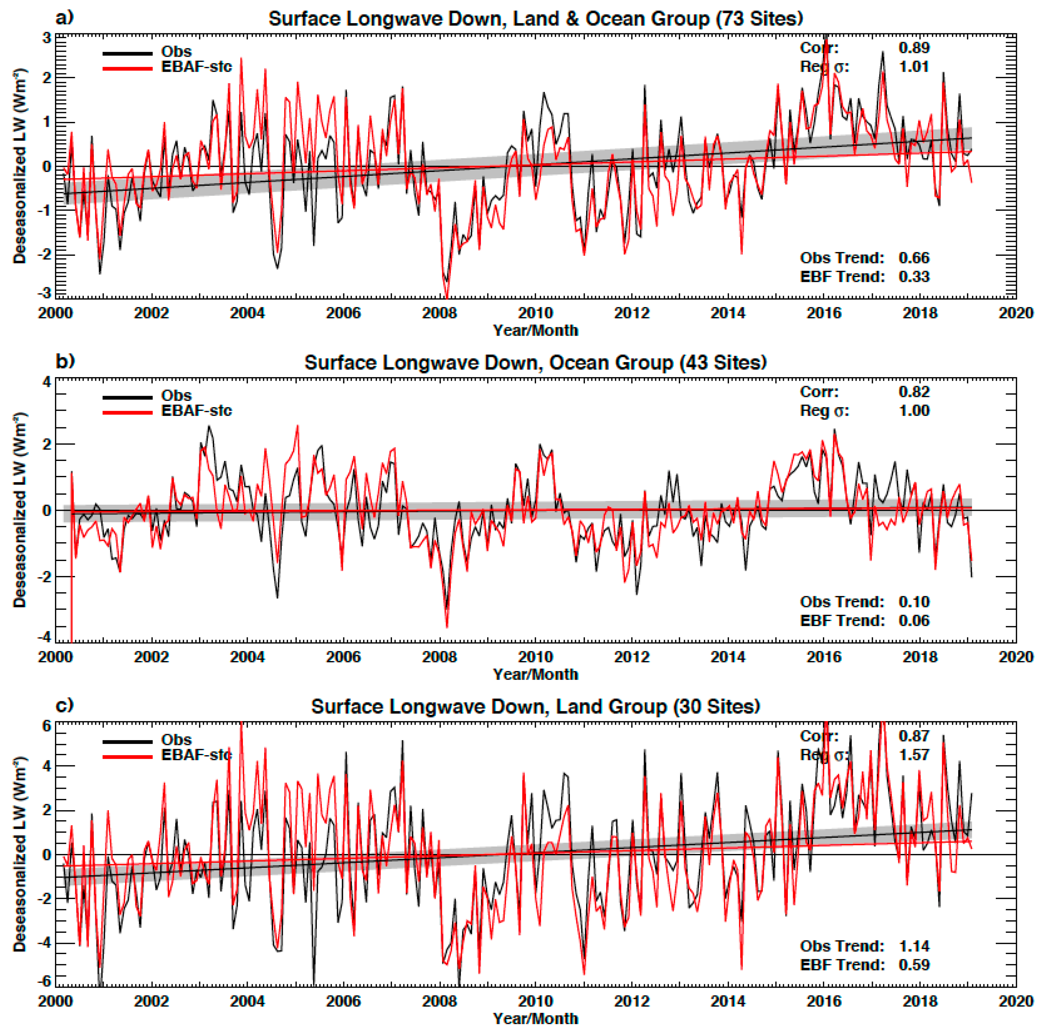
| Longwave | 1.015 | 0.478 | 0.889 | 0.66 | 0.89 | 0.44 | 0.33 | 0.57 | 0.09 |
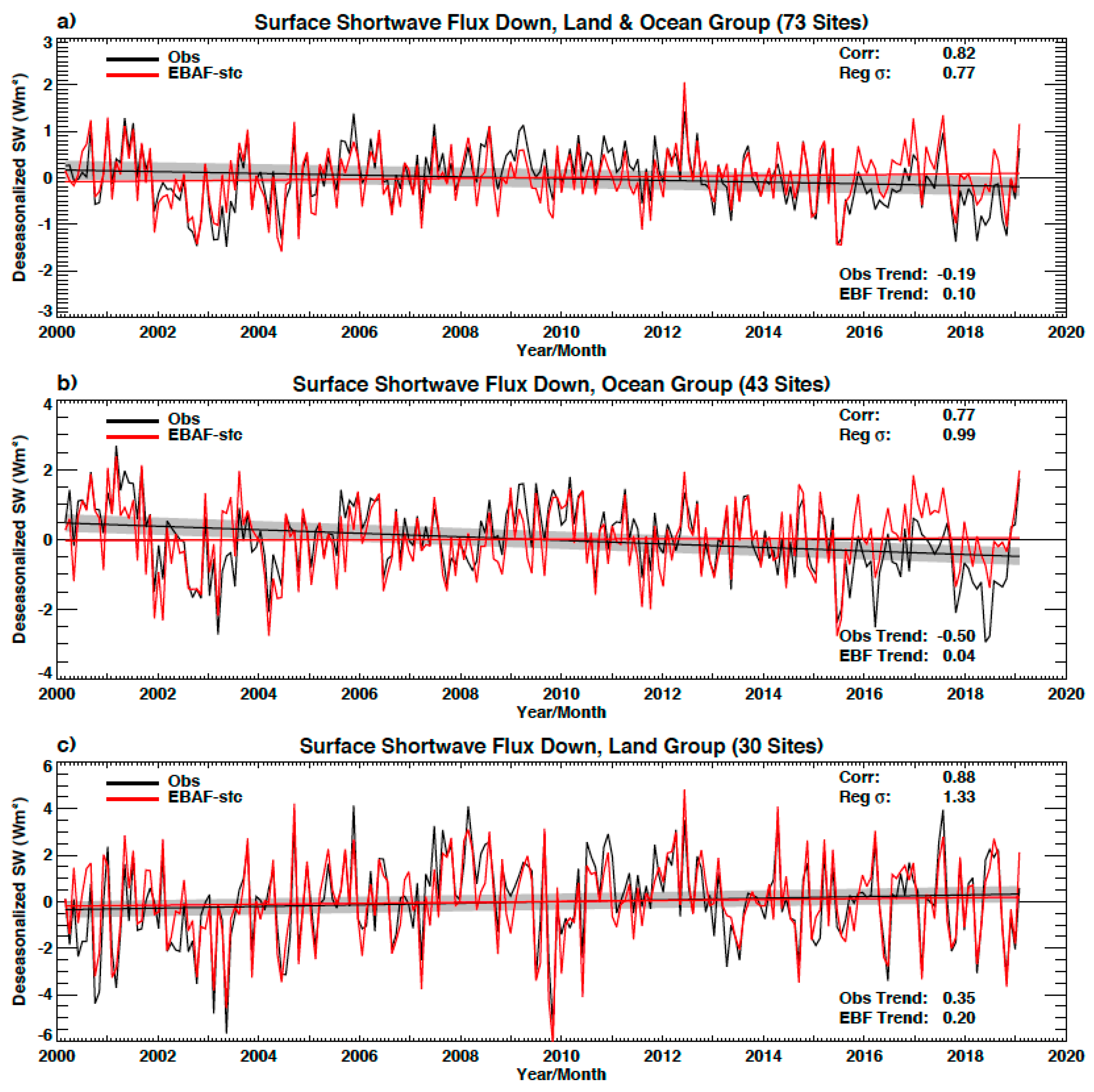
| Shortwave | 0.773 | 0.464 | 0.820 | −0.19 | −0.00 | −0.37 | 0.10 | 0.28 | −0.09 |
| Ocean | |||||||||
| Longwave | 0.996 | 0.590 | 0.825 | 0.10 | 0.34 | −0.14 | 0.06 | 0.30 | −0.18 |
| Shortwave | 0.991 | 0.668 | 0.773 | −0.50 | −0.28 | −0.73 | 0.04 | 0.28 | −0.19 |
| Land | |||||||||
| Longwave | 1.572 | 0.801 | 0.870 | 1.14 | 1.48 | 0.79 | 0.59 | 0.95 | 0.22 |
| Shortwave | 1.333 | 0.655 | 0.879 | 0.35 | 0.67 | 0.04 | 0.20 | 0.52 | −0.12 |
| Downward Irradiances | |||||
|---|---|---|---|---|---|
| Land + ocean | |||||
| Longwave | −0.33 | 0.12 | 0.11 | 0.37 | 0.52 |
| Shortwave | 0.29 | 0.09 | 0.09 | 0.32 | 0.45 |
| Ocean | |||||
| Longwave | −0.03 | 0.12 | 0.12 | 0.17 | 0.24 |
| Shortwave | −0.55 | 0.12 | 0.11 | 0.57 | 0.81 |
| Land | |||||
| Longwave | −0.55 | 0.18 | 0.17 | 0.60 | 0.85 |
| Shortwave | −0.15 | 0.16 | 0.16 | 0.27 | 0.38 |
© 2020 by the authors. Licensee MDPI, Basel, Switzerland. This article is an open access article distributed under the terms and conditions of the Creative Commons Attribution (CC BY) license (http://creativecommons.org/licenses/by/4.0/).
Share and Cite
Kato, S.; Rutan, D.A.; Rose, F.G.; Caldwell, T.E.; Ham, S.-H.; Radkevich, A.; Thorsen, T.J.; Viudez-Mora, A.; Fillmore, D.; Huang, X. Uncertainty in Satellite-Derived Surface Irradiances and Challenges in Producing Surface Radiation Budget Climate Data Record. Remote Sens. 2020, 12, 1950. https://0-doi-org.brum.beds.ac.uk/10.3390/rs12121950
Kato S, Rutan DA, Rose FG, Caldwell TE, Ham S-H, Radkevich A, Thorsen TJ, Viudez-Mora A, Fillmore D, Huang X. Uncertainty in Satellite-Derived Surface Irradiances and Challenges in Producing Surface Radiation Budget Climate Data Record. Remote Sensing. 2020; 12(12):1950. https://0-doi-org.brum.beds.ac.uk/10.3390/rs12121950
Chicago/Turabian StyleKato, Seiji, David A. Rutan, Fred G. Rose, Thomas E. Caldwell, Seung-Hee Ham, Alexander Radkevich, Tyler J. Thorsen, Antonio Viudez-Mora, David Fillmore, and Xianglei Huang. 2020. "Uncertainty in Satellite-Derived Surface Irradiances and Challenges in Producing Surface Radiation Budget Climate Data Record" Remote Sensing 12, no. 12: 1950. https://0-doi-org.brum.beds.ac.uk/10.3390/rs12121950