From Monitoring to Forecasting Land Surface Conditions Using a Land Data Assimilation System: Application over the Contiguous United States

Abstract

LDAS-Monde is a global land data assimilation system (LDAS) developed by Centre National de Recherches Météorologiques (CNRM) to monitor land surface variables (LSV) at various scales, from regional to global. With LDAS-Monde, it is possible to jointly assimilate satellite-derived observations of surface soil moisture (SSM) and leaf area index (LAI) into the interactions between soil biosphere and atmosphere (ISBA) land surface model (LSM) in order to analyze the soil moisture profile together with vegetation biomass. In this study, we investigate LDAS-Monde’s ability to predict LSV states up to two weeks in the future using atmospheric forecasts. In particular, the impact of the initialization, and the evolution of the forecasted variables in the LSM are addressed. LDAS-Monde is an offline system normally driven by atmospheric reanalysis, but in this study is forced by atmospheric forecasts from the European Centre for Medium-Range Weather Forecasts (ECMWF) for the 2017–2018 period over the contiguous United States (CONUS) at a 0.2° × 0.2° spatial resolution. These LSV forecasts are initialized either by the model alone (LDAS-Monde open-loop, without assimilation) or by the analysis (assimilation of SSM and LAI). These two forecasts are then evaluated using satellite-derived observations of SSM and LAI, evapotranspiration (ET) estimates, as well as in situ measurements of soil moisture from the U.S. Climate Reference Network (USCRN). Results indicate that for the three evaluation variables (SSM, LAI, and ET), LDAS-Monde provides reasonably accurate and consistent predictions two weeks in advance. Additionally, the initial conditions after assimilation are shown to make a positive impact with respect to LAI and ET. This impact persists in time for these two vegetation-related variables. Many model variables, such as SSM, root zone soil moisture (RZSM), LAI, ET, and drainage, remain relatively consistent as the forecast lead time increases, while runoff is highly variable.

1. Introduction

Extreme meteorological and climatic events, such as heatwaves and droughts, are predicted to increase in frequency and magnitude in future decades [1,2]. These events have significant ramifications on society, leading to environmental, economic, and societal damages. In particular, droughts have been found to be a detrimental and costly natural hazard [3,4,5,6,7], accounting for around 20% of all natural hazard damages [8] and costing society billions of dollars every year [7]. Due to this large impact, it is critical to monitor and predict the land surface variables (LSV) that link drought and society [9]. The monitoring, prediction, and therefore warning of droughts, floods, famine, and other extreme events can be accomplished with land surface models (LSM) [10,11] that can simulate the LSV responses to these extreme events. These events and their responses also pose a significant scientific challenge for the adaptation to climate change [1]. Good knowledge of both land and lower atmosphere conditions is necessary to accurately monitor and predict LSV values. This understanding is also critical for the monitoring and prediction of drought. Specifically, modeling of surface soil moisture (SSM), leaf area index (LAI), and evapotranspiration (ET) is of high importance for agricultural producers in drought-prone areas [12,13,14]. While LSM simulations provide temporally and spatially continuous information about LSV, they are by no means perfect, and often lack complex interactions and physics that result in predictions differing from reality.

The availability of global LSV observations from satellite instruments enables the constraining of LSM simulations using data assimilation (DA) techniques. A number of DA systems are able to sequentially combine model variables and observations at regular and consistent intervals, as demonstrated by [15,16,17,18,19,20], among others. Many land data assimilation systems (LDAS) already exist, including the Global Land Data Assimilation System (GLDAS) [21], North American Land Data Assimilation System (NLDAS) [22,23], Coupled Land and Vegetation Data Assimilation System (CLVDAS) [24], the Famine Early Warming Systems Network (FEWS NET) Land Data Assimilation System (FLDAS) [25], and the National Climate Assessment – Land Data Assimilation System (NCA-LDAS) [26,27,28]. Barbu et al. [18] developed an offline regional LDAS over France in the research department of Météo-France (CNRM, Centre National de Recherches Météorologiques). This LDAS was able to sequentially assimilate LAI and SSM at the same time into the ISBA (interactions between soil biosphere and atmosphere) LSM [29,30,31,32]. The LDAS-Monde tool [33,34,35] is an upgraded version of this LDAS. LDAS-Monde is able to combine Earth observation data and LSM simulations at a global scale and over specific areas. It can be used for the monitoring, and possibly the prediction, of LSV conditions.

LDAS-Monde is forced by atmospheric variables and the sequential assimilation of satellite-derived LAI and SSM data produces an analysis of land surface conditions. The assimilation permits the analysis of the vegetation biomass and of the soil moisture profile. Albergel et al. [33] showed that the root zone soil moisture (RZSM) analysis benefits from the assimilation of SSM and also from the assimilation of LAI, especially in dry conditions. LDAS-Monde has been successful at representing LSV such as SSM, RZSM, LAI, gross primary production, and ET, by using atmospheric reanalysis data, such as those produced by the European Centre for Medium-Range Weather Forecast fifth generation reanalysis, ERA5. LDAS-Monde outputs result in good correlations when compared to satellite and/or in situ observations of land surface states [34,35,36,37]. So far, forecasting LSV conditions with LDAS-Monde is at a preliminary stage.

The objectives of this study are to assess to what extent (1) LSV conditions can be forecasted using an LSM, (2) LSV initial conditions influence the forecasts, (3) data assimilation can improve the accuracy of initial conditions of LSV forecasts, and (4) LSV forecasts can benefit to crop monitoring.

This study makes use of LDAS-Monde, towards the goal of moving from monitoring to predicting LSV conditions. Atmospheric forecasts are used to force the ISBA LSM to assess the forecast of LSV conditions. In situations when it is possible to predict atmospheric variables with reasonable accuracy days up to two weeks in advance, those same atmospheric predictions can be used to predict the vegetation and soil moisture variables used to characterize drought. The rationale underlying this study is that an LSM that can successfully monitor vegetation conditions forced by accurate atmospheric reanalyses would logically be able to forecast land surface conditions provided that accurate atmospheric forecasts are available. Running the LSV forecasts with atmospheric forecasts also underlines the importance of accurate initial conditions. Improving the accuracy of LSV initial conditions using data assimilation is a key issue.

The novel assessment in this study uses the LDAS-Monde data assimilation system with atmospheric forcing variables from the European Centre for Medium-Range Weather Forecasts (ECMWF) 15-day forecasts for the two-year 2017–2018 period over the contiguous United States (CONUS).

In both monitoring and forecasting modes, LDAS-Monde results are compared to several independent datasets for analyzing the accuracy of the LSV modeling and the impact of initial conditions (i.e., the impact of the data assimilation). To assess root zone and surface soil moisture simulations, an independent dataset of soil moisture measurements from the U.S. Climate Reference Network (USCRN) [38] across CONUS is used. The simulations of ET are compared to the satellite driven estimates of the Atmosphere-Land Exchange Inverse (ALEXI) [39] surface energy balance model. The LAI and SSM LDAS-Monde outputs are also compared to the matching satellite-derived products as a way to assess the correct behavior of the data assimilation impact.

Section 2 describes the materials and methods used in this study, including assimilated and verification datasets. Section 3 describes the results of the monitoring and forecast experiments by the comparison to verification datasets. Section 4 interprets and discusses these results in the context of known geographic and biophysical patterns. Finally, Section 5 summarizes and concludes this article.

2. Materials and Methods

2.1. Atmospheric Forcing

LDAS-Monde has recently been updated with the ability to also ingest forecasted atmospheric data to drive the ISBA model [35,36]. Twice daily, ECMWF runs global, 15-day, 51-member ensemble forecasts at a spatial resolution of 0.2° × 0.2°. This configuration consists of a control run (CTRL), which is an unperturbed forecast run, and 50 perturbed members. The perturbed members are similar to the control run, but with initial states and model physics slightly perturbed to explore the range of uncertainty in the model. The ensemble forecasts are commonly used as probability guides (e.g., warmer or colder than average, probability of more than a precipitation threshold, etc.) and to investigate extreme weather events (e.g., tropical cyclones, heavy precipitation). This study makes uses of the CTRL forecast with a 15-day lead time. The atmospheric forecast has an hourly timestep up to day three, a three-hourly timestep up to day six, and then a six-hourly timestep up to day fifteen. For our LSV forecast experiment, we only used the six-hourly timestep up to day 15 which we linearly interpolated to every three hours in order to match the 09:00 UTC hour start of the assimilation window.

The atmospheric variables required to force the ISBA LSM are air temperature, wind speed, air specific humidity, atmospheric pressure, shortwave and longwave downwelling radiation, and liquid and solid precipitation. All these variables are given by the ECMWF simulations, except for air specific humidity, which we calculated from air temperature and air dewpoint temperature. The unmodified atmospheric forcings were ingested into the ISBA LSM.

The different ECMWF atmospheric forcing datasets and temporal resolutions can impact the shape and amplitude of the diurnal cycle of shortwave solar radiation. These differences in solar radiation can have a large effect on ET, with stomatal changes responding directly to shortwave radiation in the ISBA LSM. To counteract these problems, the experiments were run using a downward shortwave interpolation scheme, which is intended to better capture the peak hours of solar radiation by using a calculation of the solar zenith angle at each latitude and longitude based on the time of year (http://www.umr-cnrm.fr/surfex/spip.php?article428, last accessed 12 May 2020).

2.2. Assimilated Satellite Observations

Figure 1 illustrates the domain as well as the assimilated land surface observations averaged over 2017–2018. The SSM and LAI satellite observations assimilated in this study are products of the Copernicus Global Land Service (CGLS) [40]. The SSM product is derived from the Advanced Scatterometer (ASCAT) microwave sensor aboard the polar orbiting MetOp A and B satellites [41,42]. This product is available from 2007 to present and is produced as a daily synthesis from both sensors. The soil moisture information is based on radar backscatter observations. An exponential filter [43] is then applied to this product to estimate the soil wetness index (SWI) using a timescale parameter, T, that varies between 1 and 100 days. With this T parameter, SWI accounts for other physical parameters such as soil thickness and type, soil texture and density, evaporation, and runoff. This experiment uses the smallest possible T value, T = 1 day, to best estimate the surface soil moisture (SSM), which is expressed as a percentage of saturation between 0 (completely dry) and 100 (completely saturated) of the topsoil layer. This product is global at a 0.1° × 0.1° resolution, which is interpolated to an ISBA model grid of 0.2° × 0.2°.

The SSM product that is assimilated must be rescaled to match the model climatology in units of m³ m^-3 in order to address a possible misclassification of land surface parameters such as soil porosity, wilting point, and field capacity [44,45]. The ASCAT SWI product is transformed into the model-equivalent SSM with the linear rescaling method as described in [46], where the observations’ mean and variance are matched to the modeled surface soil moisture mean and variance. The second layer of soil in the ISBA model (WG2, 1–4 cm depth) is used to represent the topsoil properties. This rescaling gives, in practice, very similar results to cumulative distribution function (CDF) matching. The linear rescaling is performed on a seasonal basis (with a three-month moving window) as suggested by [16,17,18]. The rescaling parameters were derived monthly and screened for the presence of ice and urban surfaces. Average observed SWI over CONUS for 2017–2018 is displayed in Figure 1. The SSM observational dataset is filtered to exclude pixels whose average altitude is above 1500 m above sea level and pixels whose land cover fraction exceeds 15% of urban surfaces.

Over the considered period, 2017–2018, the assimilated LAI observations are derived from the PROBA-V (2014–present) mission. This study uses the GEOV2 dataset, which applies the observations to a 1 × 1 km spatial resolution with data steps every 10 days [47]. These observations are then also interpolated to the 0.20° × 0.2° model grid. Averaged LAI observations for 2017–2018 are displayed in Figure 1.

2.3. Independent Evaluation Datasets

USCRN is a National Oceanic and Atmospheric Administration (NOAA) network of climate-monitoring stations. USCRN contains 114 sites with hourly soil moisture and temperature measurements at 5, 10, 20, 50, and 100 cm depths, relatively well spread over CONUS. In order to effectively evaluate LDAS-Monde’s ability to predict surface variables, the SSM simulations are compared to observed data at all sites with continuous quality-controlled data for all of 2018 in the USCRN over CONUS. The number of these sites differs based on the individual layer of soil moisture. This study uses two layers of measurement from USCRN, the 5 and 20 cm observations. The 5 cm layer is compared to ISBA soil layer 3 (WG3) representing 4–10 cm depth, while the 20 cm observation is compared to an average of ISBA layers 4 and 5 (WG4 and WG5) representing 10–20 and 20–40 cm, respectively, weighted by each layer’s respective thickness.

ALEXI [39,48,49,50] is a surface energy balance model calculating ET based on a two-source land surface representation of the energy budget. The model treats the land surface as a combination of soil and vegetation with unique fluxes, temperatures, and coupling with the atmosphere. This single model formulation can be applied to wide ranging moisture and vegetation conditions, including partially vegetated surfaces. ALEXI is produced at both the global scale and over CONUS at 0.05° × 0.05° and 0.04° × 0.04° spatial resolution, respectively. This independent dataset is used to evaluate LDAS-Monde’s parameterization of ET processes.

2.4. LDAS-Monde

Within the SURFEX (Surface Externalisée Version 8.1) modeling system [51] developed by CNRM (http://www.umr-cnrm.fr/surfex), a package allows the assimilation of satellite-derived products into the ISBA land surface model using the LDAS-Monde data assimilation system. LDAS-Monde is a global scale LDAS, with options to couple to hydrological models. LDAS-Monde also provides statistics that can be used to monitor the impact of the assimilation of satellite observations. The specific components of the system are detailed below.

The LSM used in this study is the CO₂-responsive [30,31,32], multi-layer soil [52,53] version of the ISBA model. This version of the model allows the representation of vegetation biomass and LAI, in addition to exchanges in CO₂, energy, and water fluxes between the surface and the atmosphere. In our configuration, ISBA uses 12 predefined land surface patch types including nine functional plant types (needle leaf trees, evergreen broadleaf trees, deciduous broadleaf trees, C3 crops, C4 crops, C4 irrigated crops, herbaceous, tropical herbaceous, and wetlands) as well as bare soil, rocks, and permanent snow and ice surfaces. These patches are extracted from ECOCLIMAP Second Generation [54], an evolution of ECOCLIMAP-II [55]. Urban surfaces defined in ECOCLIMAP-SG are converted to bare rock when running ISBA alone. Atmospheric, climatic, and land use conditions create the evolution in the vegetation biomass through processes of plant growth and mortality. During growth phases, increased photosynthesis results in CO₂ assimilation, creating vegetation growth and increasing LAI from the minimum threshold (which is 1 m² m⁻² for evergreen forests and 0.3 m² m⁻² for all other types of vegetation). The experiments presented in this paper use a 14 layer, 12m depth soil diffusion scheme, with layers at 0.01, 0.04, 0.1, 0.2, 0.4, 0.6, 0.8, 1, 1.5, 2, 3, 5, 8, and 12 m depths [56].

In the LDAS-Monde system [33], observed satellite LAI and SSM data are assimilated into the ISBA LSM using a simplified extended Kalman filter (SEKF) DA technique [57]. The SEKF technique uses finite differences to compute the flow dependency between the assimilated observations, SSM and LAI, and the control variables (soil moisture from layer of soil 2 to 8 (1 cm to 100 cm) and LAI). The eight control variables are directly updated by the observed variables according to their sensitivity as given by the SEKF Jacobian matrices [19,33,58]. Other model variables are updated indirectly through feedbacks and other biophysical processes as related to the control variables. The SEKF technique used in this study is the most mature data assimilation scheme currently implemented in LDAS-Monde. Bonan et al. [59] recently implemented and validated an ensemble-based Kalman filter.

2.5. Experimental Setup

In this study, the LDAS-Monde offline system is used in a forecast mode, forced by ECMWF atmospheric forecasts over the CONUS domain. It produces one- through 14-day LSV forecasts for each day in the 2017–2018 period. The maximum 14-day lead time corresponds to potential changes in LSVs’ conditions impacting agricultural decisions such as the timing of irrigation, planting, and harvesting. The LSV forecasts are initialized by either the open-loop (OL) and by the analysis resulting from the DA experiment based on the sequential use of the SEKF to assimilate SSM and LAI. The OL corresponds to model-only simulations, without data assimilation. The OL- and SEKF-based forecast runs differ by changing their initialized conditions, with SEKF having what should be a more accurate initial state due to the assimilation of observations. The CONUS domain is defined as longitude 130° W to 60° W and latitude 55° N to 20° N.

Table 1. Description of the LDAS-Monde data assimilation (DA) experiment used in this study.

Model	Domain	Time Scale and Model Resolution	Atmospheric Forcing	Deterministic Atmospheric Forecast	Assimilated Observations	Model Equivalent of Observations	Control Variables
ISBA Multi-layer soil Plant growth (“NIT” option in SURFEX)	CONUS (20N–55N, 130W–60W)	2017–2018, 0.20° × 0.20°	CTRL first 24 h (3–hourly)	Up to 15 days	SSM (ASCAT) LAI (GEOV2)	Rescaled WG2 (1–4 cm) LAI	Layers 2 to 8 (1–100 cm) LAI

presents the characteristics of the DA experiment. LDAS-Monde uses a 24 h assimilation window from 09:00 UTC to 09:00 UTC next day. The atmospheric forecast forcings begin at 00:00 UTC while ISBA begins running at 09:00 UTC. This discrepancy causes the 15-day atmospheric forecast to produce only 14 full days of data. For this forecast experiment to reach an equilibrium able to generate physically realistic initial conditions, the first year (2017) was spun up 20 times using the earliest time period of the CTRL member of the ECMWF ensemble forecast (FC1, corresponding to the first day of forecast) as atmospheric forcing.

Since previous studies [33,34,35,36,37] have demonstrated that LDAS-Monde analyses can accurately represent LSVs, this study uses a novel approach regarding the assessment of the forecasted variables. The SEKF at FC1 is used as a reference. If the variables do not change greatly between later forecast periods and FC1, it can be said that forecast variables are persistent. This persistence is important to find as highly different values should encourage more scrutiny for that variable, whereas highly similar values can be treated like the reanalysis (i.e., no forecast).

2.6. Assessment

Two scores are considered in this study: the Pearson’s correlation coefficient (R) and the root mean squared difference (RMSD).

For surface soil moisture, score values between in situ observations and modeled soil moisture are only calculated when soil temperatures (as given by USCRN measurements) are above 4 °C to avoid frozen conditions. The ISBA LSM separates liquid and solid soil moisture, and the simulated SSM variability can be affected by soil freezing when the modeled soil temperature is close to the freezing level. Correlations are only calculated when there are more than 100 days of soil moisture measurements in the 2017–2018 timeframe above this 4 °C threshold. Correlations are only retained when the p-value is less than 0.05 (i.e., scores are significant at P values < 0.05).

The normalized information contribution (NIC) is defined by Equations (1) and (2) as in [60]. The NIC provides a metric to quantify the improvement or degradation from the analysis compared to the model. It is computed for the correlations, and for RMSD (Equations (1) and (2), respectively): R_Analysis (RMSD_Analysis) is the correlation coefficient (RMSD) between the SEKF experiment and observations, while R_Model (RMSD_Model) is the correlation coefficient (RMSD) between the OL experiment and observations. While the average NIC_R and NIC_RMSD values over all the stations are simple and good indications of overall trends, the effect of the assimilation on individual stations can be highly variable. This is important to note if work is done at a more local or regional level as the CONUS average may not represent each individual station. These normalized scores are used in assessments using satellite observations of LAI, SSM, and ET. For NIC_R, positive values indicate improvement from the assimilation, while negative values indicate degradation. For NIC_RMSD, this pattern is reversed, with negative values denoting improvement from the assimilation, and positive values denoting deterioration.

$$NI{C}_R^{}=\frac{R_{Analysis}-R_{Model}}{1-R_{Model}}\times 100$$

(1)

$$NI{C}_{RMSD}^{}=\frac{RMS{D}_{Analysis}-RMS{D}_{Model}}{RMS{D}_{Model}}\times 100$$

(2)

Finally, the bootstrapping statistical approach is used in order to calculate 99% confidence intervals and to determine statistically significant differences between the model and analysis with regards to forecast time period. The bootstrapping method can be summarized by the repeated random removal of points and recalculation of the desired variable. In this analysis, this removal process is repeated 10,000 times in order to generate a sufficiently large number of samples in order to find 99% confidence intervals. Bootstrapping was applied to the correlation values of all evaluation datasets (CGLS SSM, CGLS LAI, ALEXI ET, and USCRN in situ soil moisture) versus matching OL and SEKF variables.

3. Results

3.1. Impact of the Analysis

Analysis increments, given in Figure 2, are the amount of daily mean change in each variable from the assimilation of observations. These demonstrate the effect that the assimilation of LAI and SSM has on five of the control variables (LAI, WG2–WG5 representing soil moisture layers 1–40 cm). Specifically, it gives the average LAI (m² m⁻²) or volumetric soil moisture (m³ m⁻³) added or removed from the model run due to the assimilation over the considered 2017–2018 period. LAI experiences the strongest effect, with negative LAI increment values being observed over most of the domain, most strongly in the Great Plains, Midwest, and Eastern U.S. One distinct pattern is the Mississippi River valley, where LAI is more markedly decreased. The coastal Pacific Northwest is the main region with the opposite reaction, instead adding to the LAI. The model-equivalent of SSM, at 1–4 cm depth (WG2), has a more diverse reaction to the assimilation, with significant areas where water is added, mostly in the southwest and southern Texas, and where it is removed, predominantly in the Washington, Oregon, Idaho, and Nevada areas. Much of the domain also has a weak or neutral change. Increments at 10 cm (WG3) (Figure 2c) are generally still removing soil moisture, with some areas strongly removing, and scattered, weaker areas of adding soil moisture. Soil layers at the 20 and 40 cm depths (WG4 and WG5, respectively) have increments (Figure 2d–e) in a more uniform pattern, with nearly all regions having soil moisture removed.

3.2. Persistence: Forecast Versus Initial Conditions

In this section, all SEKF-initialized forecast lead times are compared to the initial condition of the analysis produced by the assimilation (i.e., the SEKF) in order to assess each variable’s persistence in time. Understanding this persistence was done as an initial step towards understanding the persistence of the system as in a forecast mode. This analysis provides a standardized comparison to determine the persistence of each variable in the LSM. Calculations of average correlation and RMSD for five LSVs (LAI, WG2, RZSM, Runoff, Drainage, and ET) are given in Figure 3. As these correlations and RMSD are compared to the initial conditions at FC1, the statistics would be in perfect agreement at that time step (comparing FC1 against itself). Due to this, RMSD in Figure 3 is shown as a percentage change from the FC1 initial condition. The individual RMSD for the LSVs follow the same general pattern. The LAI, RZSM, WG2, and drainage variables all remain within 20% of the initial condition at FC14. Unlike correlation, ET quickly increases RMSD and at FC14 is ~88% higher than its initial condition. Finally, runoff changes the quickest and finishes at over 210% changed from the initial condition. All correlations decrease as the forecast period increases, but at different rates per variable. For instance, the LAI and RZSM correlations are nearly identical in their decrease, barely having diminished at the fourteen-day forecast time. Drainage decreases in correlation slightly more with values dropping 0.1 by forecast day 14. The WG2 and ET correlations diminish more rapidly, both decreasing by approximately 0.2 over the fourteen days of lead time. Finally, the runoff correlation quickly falls, of about 0.3, between forecast day 11 and day 14.

3.3. Evaluation Using Satellite-Derived Products

LDAS-Monde has the ability to ingest atmospheric forecasts in order to output forecasts of land surface conditions. Presented here are the results of comparing LDAS-Monde-forecasted SSM, LAI, and ET to the satellite-derived evaluation datasets of the same variables. This analysis is not only focused on how the forecasts perform in a general sense (i.e., how accurate are these predictions 14 days in advance), but also focuses on the impact of the initialization, that is, if the forecast is initialized by the OL or SEKF. The correlations and RSMD values for SSM, LAI, and ET are summarized in

Table 2. Impact of forecast lead time and initialization on the prediction of surface soil moisture (SSM), LAI, and ET by LDAS-Monde over the CONUS, during the 2017–2018 time period. Only even values of forecast lead times are indicated, from 2 to 14 days (FC2 and FC14, respectively). The R values smaller than 0.5 and the SSM RSMD values larger than 0.05 m³ m⁻³ are in bold.

LSV	Initialization	Score	Forecast Lead Time
			FC2	FC4	FC6	FC8	FC10	FC12	FC14
SSM	OL	R RMSD (m3 m−3)	0.62 0.044	0.58 0.046	0.52 0.050	0.46 0.053	0.41 0.056	0.36 0.059	0.35 0.060
	SEKF	R RMSD (m3 m−3)	0.64 0.042	0.59 0.046	0.53 0.049	0.46 0.053	0.41 0.056	0.36 0.059	0.34 0.060
LAI	OL	R RMSD (m2 m−2)	0.56 1.02	0.55 1.02	0.55 1.01	0.57 1.01	0.56 1.01	0.56 1.01	0.55 1.01
	SEKF	R RMSD (m2 m−2)	0.69 0.73	0.69 0.73	0.69 0.73	0.71 0.73	0.71 0.73	0.65 0.82	0.64 0.82
ET	OL	R RMSD (mm day−1)	0.57 1.37	0.57 1.37	0.57 1.37	0.56 1.39	0.55 1.40	0.54 1.40	0.54 1.42
	SEKF	R RMSD (mm day−1)	0.58 1.35	0.58 1.35	0.58 1.36	0.57 1.38	0.56 1.39	0.55 1.39	0.55 1.40

. The bootstrapped 99% confidence intervals of correlation (not shown) range from ± 0.001 to ± 0.003 for SSM (either OL or SEKF), ± 0.003 to ± 0.004 for LAI (either OL or SEKF), and ± 0.002 to ± 0.003 for ET (either OL or SEKF). The temporal correlations of SSM, LAI, and ET to the satellite-derived observations for FC1 are given in Figure 4 together with NIC_R, with red colors representing improvement from assimilation, and blue representing degradation. The RMSD score and NIC_RMSD are given in Figure 5 with blue colors for NIC_RMSD representing improvement from the assimilation, and red representing degradation. Results for SSM, LAI, and ET are further described in Section 3.3.1, Section 3.3.2, and Section 3.3.3, respectively.

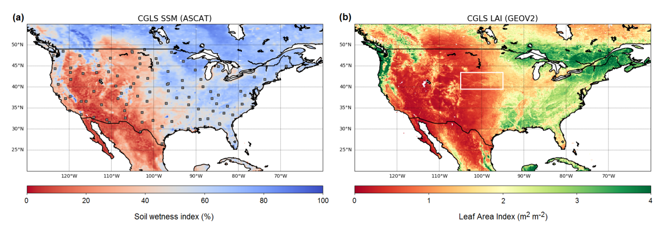
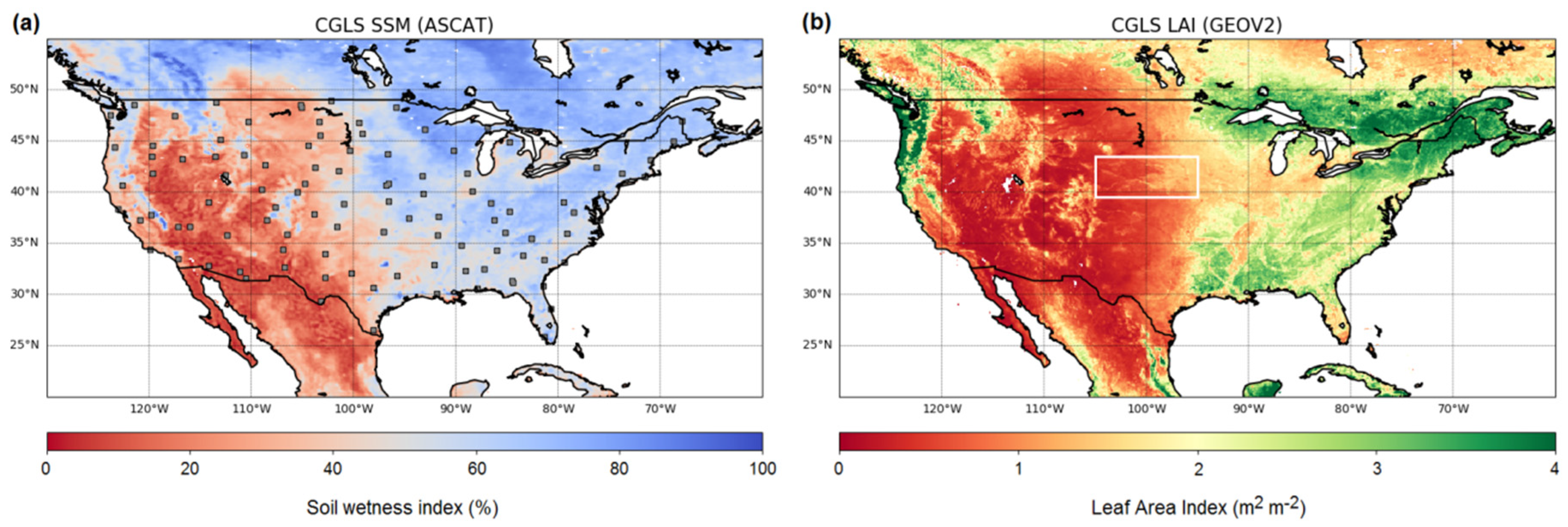
3.3.1. Surface Soil Moisture

Figure 4 shows that SSM temporal correlations are generally very high across much of the continent, with some particularly dry areas, specifically in the U.S. Southwest and southern Texas, having far lower values. The NIC_R values show the visible improvement of correlation values by the assimilation in much of the domain, including the entire Western U.S., much of the central Great Plains, and a large portion of the Midwest. Few, if any, parts of the domain show any degradation after assimilation. The RMSD values of SSM are shown in Figure 5. There are some regions of locally higher RMSD, specifically in the Midwest and eastern Great Plains including some southern states, and additional pockets of high error in portions of the Pacific Northwest, some of the Rocky Mountains, and much of Canada. The data assimilation lowers this error in much of the Southwest, Pacific coast, and Montana, with a more moderate reduction in the Midwest. The lower Mississippi River valley is also outlined by a reduction in error. Scattered patterns of higher RMSD can be seen in some of the mountainous Northwest and Wyoming areas. The average correlation and RMSD for SSM for each forecast period using both model (OL) and analysis (SEKF) initializations are given in Table 2 and in Figure 6. Both OL- and SEKF-initialized correlations experience a consistent drop as the forecast period increases, with correlations at forecast day 14 around 50% lower than the first day of forecast. At the FC1 lead time, the OL correlations start at 0.63 (± 0.003), while SEKF correlations begin at 0.66 (± 0.0025) and are significantly higher than OL until FC5, where the analysis and model are nearly identical. From FC6 to FC14, the two initializations have similar values, with correlations of both ending at FC14 of about 0.35 (± 0.003). Likewise, the RMSD shows a consistent increase (degradation) as the forecast moves forward, with the model having either a slightly higher value or exactly the same error, as far as the output precision allows. As with correlation, the first few days of forecast see RMSD values that have a larger difference between the OL- and SEKF-initialized states compared with the mid length and later forecast days. From FC8 to FC14, the mean SSM R (RMSD) values are smaller (larger) than 0.5 (0.05 m³m⁻³). The OL and SEKF initialization modes give very similar R and RMSD values from FC8 to FC14. The 99% confidence intervals determine that the OL and SEKF initializations from FC1 to FC4 are significantly different, whereas the rest of the forecast period do not see statistically different values based on the initializations. These results denote a poor predictability of SSM beyond less than a week forecast lead time.

In order to see the geographic patterns of the SEKF and OL initialization differences, maps of NIC_R and NIC_RMSD are presented for FC2, FC8, and FC14 in Figure 7. The SSM NIC_R shows how over much of the US, the early forecast lead times see strong improvement (positive, red) across the domain, with strongest improvements in the dry Southwest as well as in the northern Great Plains. As the forecast lead time increases, some areas still show strong improvement, with the Southwest remaining strongly influenced by the initialization out to FC14. Additionally, after the eight-day lead time, there is a small pocket of reduced correlation found at the Washington–Oregon state border, which is not present in earlier lead times, becoming more negative at FC14. Over the entire domain, the magnitude of improvement markedly decreases with the forecast lead time, reducing it to almost equally low positive and negative impact at 14 days. Further shown in Figure 7 is the NIC_RMSD for SSM presenting a similar pattern of improvement (negative, blue) and degradation (positive, red). The Washington–Oregon border shows degradation at earlier lead times than for correlation, while much of the other domain indicates the analysis initialization improves error. The Southwest patch also stands out with particularly strong and lasting improvements. As the lead time increases, these effects are reduced in magnitude, but even at 14–days lead time, those two patches are distinguishable. As with correlation, a general reduction in error over the domain is most prominent only in the two-day lead time, and after it is reduced to near equal improvement and degradation.

3.3.2. Leaf Area Index

Temporal correlation maps for LAI at the FC1 lead time are given in Figure 4 with impacts from the assimilation given in Figure 5. Correlations are generally very positive over much of the central East Coast, Midwest, and Great Plains. In the mountainous and Western U.S., the correlations are more sporadic, highly variable between very high and low correlations. The impact of the assimilation is overall positive, increasing the correlation significantly in most areas, except for degradation that occurs strongly in the Southwest, and in some mountainous areas of Colorado and Utah. Figure 5 shows that RMSD has particularly high values around the lower Mississippi River, much of Appalachia, New England, and Florida. Unlike correlation, impacts on the RMSD from the assimilation are almost entirely improvements. The biggest changes occur in the Great Plains, mountainous Pacific Northwest, Florida, and again the lower Mississippi River. Smaller improvements are made in more error-prone areas such as Appalachia and New England. It is important to note the scale on the LAI improvements in correlation and RMSD from the assimilation is far larger than both SSM and ET due to the larger differences. The maximum error is also large, reaching up to 2.4 m² m⁻². Importantly, the Midwest and Great Plains, strongly agricultural regions, show very strong improvement from the assimilation, particularly in correlation, along with a distinct patch of the lower Mississippi River.

Spatially averaged LAI correlations and RMSD are given in Table 2 and Figure 6. The SEKF statistics are significantly improved compared with the OL-initialized states at all forecast steps. The OL correlations stay more or less constant at all forecast periods. The LAI RMSD values for the model indicate a similar pattern of little change. The analysis correlations do experience a strong decrease between forecast day 10 and day 11. The same pattern is seen in reverse with an analysis RMSD increase during this same period. With regards to spatial statistics for different forecast lead times (Figure 8), most of the domain experiences improvement, with NIC_R values often greater than 0.5 and NIC_RMSD often less than -0.25. Particularly, the Northeast, Midwest, and Great Plains show consistent and strong improvement at all forecast lead times. There is also weaker degradation in a belt across Mississippi, Alabama, and Georgia that becomes stronger degradation as the lead time increases. Generally, these impacts persist well through the forecast lead time, although like all other variables, they do decrease intensity somewhat. Even at 14–days lead time, the initialization by the analysis shows strong improvement in LAI correlations in much of the agricultural areas of the U.S. A similar trend is seen with NIC_RMSD. The strong improvement in the Mississippi River valley is still easy to see. The degradation in correlation seen in the Southwest is closer to no change in NIC_RMSD. Finally, the improvements in RMSD appear to fade quicker than NIC_R as the forecast lead time increases.

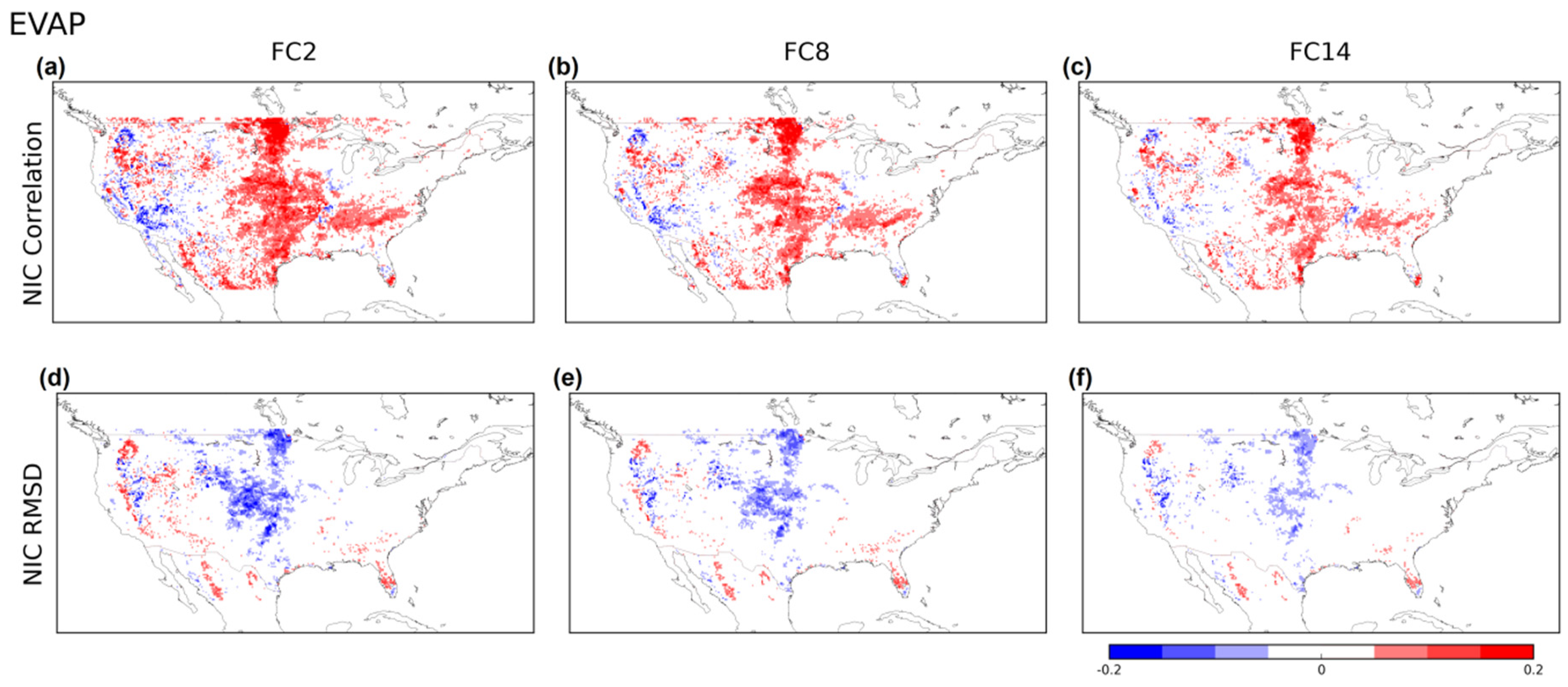
3.3.3. Evapotranspiration

Spatial correlations with ALEXI ET at FC1 (Figure 4) show strong agreement over the Midwest and some of the Great Plains. Much of the East Coast and South also demonstrated relatively strong agreement. Impacts from the assimilation indicate improvement over almost the entire Central U.S., with another area of strong improvement in the Kentucky and Tennessee regions. Some scattered degradation is seen in the West, most notably at the California, Arizona, and Nevada border. The ET RMSD and NIC_RMSD impacts are given in Figure 5. The error is largest in the South, Pacific Coast, and New England, with most of the Midwest and Great Plains having a mild RMSD. A very low RMSD occurs in the dry Southwest, areas where correlations are also very low. The NIC_RMSD demonstrates that the impacts are not as widespread as they were with correlation. The strongest improvement is in the Great Plains states of Kansas, Nebraska, South Dakota, and North Dakota. Degradation up to NIC_RMSD = 0.15 is most notably seen in the Sierra Nevada and Cascade Mountains.

With the spatially averaged correlations and RMSD of ET (Table 2, Figure 6), both the OL- and SEKF-initialized experiments show a consistent, but small, decrease in correlation as the forecast lead time increases, beginning at 0.57 (± 0.003) and 0.58 (± 0.002), respectively, and ending at the 14–day lead time at 0.54 (± 0.0025) and 0.55 (± 0.002), respectively. The RMSD values of ET forecasts initialized with OL and SEKF increase as the forecast period increases, beginning with 1.37 and 1.35 (mm day⁻¹) and ending at the 14-day lead time with 1.42 and 1.40, respectively. At all forecast lead times, SEKF-initialized runs always have significantly improved correlations and RMSD compared with the OL-initialized runs.

Figure 9 shows that the geographic patterns in the forecast time periods show that impacts on ET correlation from the assimilation are most persistent in the Central U.S. While the magnitude of these improvements does decrease, they are still evident, and in the same pattern, at FC14. With NIC_RMSD, most patterns are similar. The area of strongly improved RMSD in the central and northern Great Plains can be said to persist through the forecast lead time, but diminishes far more at FC8 and FC14 compared with the improvements in correlation.

3.4. Evaluation Using In Situ Soil Moisture Observations

At 5 cm, with 106 USCRN stations of data, the initialization makes little impact, with OL- and SEKF-initialized correlations to in situ measurements showing no significant differences. Increasing the forecast lead time logically decreases the correlation with in situ measurements, with the lowest correlation at the longest lead time as shown in Figure 10. Correlations for both initializations begin at approximately 0.74 and diminish as the forecast lead time increases, reaching a minimum below 0.50 at FC14. At the 20 cm depth, with 84 stations worth of data, the initializations do cause a visible systematic difference at early lead times, with correlations of OL and SEKF at FC1 of 0.68 and 0.69, respectively. There is also a trend of the OL- and SEKF-initialized correlations becoming closer as the lead time increases (i.e., impact of the initialization decreases with the forecast lead time). These visual differences, however, are not significant as determined by the bootstrap calculations. The 20 cm depth begins with lower correlations than the 5 cm depth but also decreases slower as the lead time increases. However, past FC8, the correlations at 20 cm are better than their 5 cm counterparts, ending at FC14 with R = 0.51 for the OL and SEKF initializations.

4. Discussion

4.1. Can LSV Conditions Be Forecasted Using a LSM?

The correlations of evaluating the forecast periods against their initial SEKF reference conditions suggest that most LSV (except for runoff) are rather persistent in time in the model. LAI and RZSM had minimal changes from forecast lead time day 2 to 14 (FC2 to FC14), indicating that, working together, the model and forecasts limit the variability of these variables. ET, WG2 (1–4 cm soil moisture), and drainage have slightly more variability, but still had very similar results between the monitoring mode and 14–day forecast. Runoff, on the other hand, varied greatly as the forecast period increased. This behavior tends to demonstrate the variable’s high degree of coupling with precipitation [61], which is a highly variable forecast variable.

From FC1, RMSD had a far greater relative change than correlation. The LAI, WG2, RZSM, and drainage all have very small changes out to FC14. ET RMSD is at least 50% higher than the previous variables at all forecast lead times. Further, like correlation, the runoff RMSD quickly decouples from the SEKF initial condition. These results show that forecasted LAI, SSM, RZSM, as well as ET and drainage can be considered rather similar to their non-forecast, SEKF, counterparts. However, run-off differs greatly and its variability indicates that we should not treat the forecasted values the same as their non-forecast counterparts.

4.2. Do LSV Initial Conditions Influence Their Forecasts?

The results of this experiment demonstrate that the influence of the initial condition on the LSV forecast depends on exactly what the LSV in question is, as well as the evaluation dataset. For example, the evaluation of SSM using USCRN in situ observations resulted in no discernible difference between the OL and SEKF initial conditions at 5cm, and a small, but not significant difference at 20cm.

At 5 cm depth, averaged LDAS-Monde OL- and SEKF-initialized correlations to the in situ observations did not significantly differ at 5 cm depth for any forecast period. Still, the correlations at FC1 generally agree with other similar comparisons such as [34], with the main difference being that this study only uses a two-year time period. This could be caused by a few different factors. First is the relatively short time period. Due to the ensemble forecast data only being used from 2017 onward, a longer period of study is not possible in this forecast capacity. The two-year analysis may not be enough time for any statistical differences to appear. Another reason is the relatively small impact of the assimilation of SSM, especially when compared with the impact of the LAI assimilation, which is discussed in the next paragraph. Notably, at FC4, the forecast of SSM is still higher than 0.70, indicating some persistence of model skill as the forecast lead time increases.

At the 20 cm layer, the initialization shows a visible, however not significant, difference. This can be caused by the impact from the assimilation of LAI, which strongly affects deeper layers of soil moisture (20 cm or deeper, ISBA equivalent WG4 and deeper) compared with SSM (1–10 cm, WG2 and WG3 ISBA equivalent) as demonstrated by [33,62]. The correlation at deeper layers is still less than at the surface, which may be explained by the lower amount of variability in the observations, leading to a lower correlation score. As seen in other instances of assimilating soil moisture [63], the neutral impact of the assimilation of ASCAT data can be partially explained by the generally high quality of LDAS-Monde OL soil moisture, compared with the quality of ASCAT. When compared directly with the ASCAT-based SWI product, observations are far less correlated with the same in situ observations (R = 0.56), while LDAS-Monde OL and SEKF initializations at FC1 show higher values (R = 0.74 for both). More research is planned to investigate the individual effects of assimilating SSM and LAI separately in order to quantify their added value independent of one another.

For forecasts in general, as the forecast period increases, the forecast skill of the LSM decreases. With a fast-evolving variable such as SSM, the model decreases in skill in a similar manner as the period increases. SSM is shown to be strongly sensitive to atmospheric conditions, and as the quality of those forcings decreases (as lead time increases), the correlations with measurements decrease. Deeper layers of soil moisture are still strongly connected to precipitation, but have less variability, leading to a slower decrease in correlation with the forecast period.

Using the CGLS SSM, differences were shown at early forecast periods, but this influence became smaller and smaller until disappearing at longer time forecast periods. The other variables of LAI and ET always resulted in differences corresponding to the initial conditions.

4.3. Can Data Assimilation Improve the Accuracy of Initial Conditions of LSV Forecasts?

Previous experiments using LDAS-Monde [33,34,62] showed that assimilated LAI and SSM satellite-derived products increase their correlations and decrease RMSD with LDAS-Monde LAI and SSM after data assimilation, averaged over the domain. This is a good check to be sure that the data assimilation is working as intended. The response of ET to the data assimilation is of special importance due to its independence from the assimilated datasets. Furthermore, the analysis of how these statistics evolve as a function of forecast lead time is a question of interest (i.e., how long do these variables provide useful, usable information). Several previous studies have looked at the impact of initial conditions on LSVs. Wood and Lettenmaier [64] found that accurate initial conditions and future atmospheric forcings are critical for good streamflow predictions. Shukla et al. [65] demonstrated similar results linking better initial conditions to improved hydrologic forecasts. Sawada et al. [66] have used CLVDAS, assimilated microwave brightness temperature and general circulation model (GCM)-based seasonal meteorological forcings, to predict LAI and agricultural drought with up to a three-month lead time. That study also found that initial conditions play an important role in the prediction of LAI. This study with LDAS-Monde differentiates itself by operating on smaller temporal scales, with operational 15–day meteorological forecasts to ensure the most accurate atmospheric forecasts available. Shorter, but more accurate atmospheric forecasts may provide useful information to stakeholders and influence their decision-making, notably for planting, irrigation, and harvest, which may require higher certainty to take action. Even on the shorter timescales, the results corroborate the idea that the initial conditions are improved after data assimilation, and that these better initial conditions contribute to more accurate forecasts for LSVs. As in [66], the strongest improvement is seen in LAI. In models coupled with the atmosphere, more accurate initial conditions through the use of data assimilation of Earth observations can also feed-back and create better forecasts of atmospheric weather patterns [67,68]. An application where LDAS-Monde would run coupled with an atmospheric model would prove useful, in particular to assess the role of vegetation.

Some geographic patterns of NIC_R and NIC_RMSD for LAI and SSM at FC1 can also be seen in the maps of analysis increments (Figure 2). Stronger improvements in correlation are generally associated with stronger increments. For example, with SSM NIC_R and NIC_RMSD (Figure 7), we see degradation in some areas of the Pacific Northwest that worsen with the forecast time. This same area is where the analysis increments show that water is removed in the model-equivalent soil layer, WG2 (1-4 cm). This may suggest that the removal of water from the assimilation may be an oversensitivity to the SSM observations. This large change, which may result in slightly improved monitoring at FC1, cascades to become less correlated and with more error at later forecast times. Additionally, average SSM correlations and RMSD (Figure 6) worsen quickly with forecast time, demonstrating the fast-evolving nature of this variable. As accurate atmospheric reanalyses are important to successfully monitor LSVs, specifically those linked to the terrestrial water cycle such as SSM [34], the same reasoning can be extended to include the importance of accurate atmospheric forecasts, in this case, up to 14–days lead time. Finally, the SEKF assimilation does prove to provide significantly more accurate initial conditions, and thus more accurate forecasts for at least some days before the OL- and SEKF-initialized SSM converge.

Correlations and RMSD to the satellite-derived LAI product from the SEKF-initialized forecasts are consistently and significantly better than the OL-initialized counterpart. This strong change driven by the assimilation corrects for model biases in the seasonal timing of vegetation peak and senescence, as well as accounting for known shortcomings such as not considering any human impacts on vegetation, such as irrigation and harvests. As with SSM, LAI using the SEKF-initialized state proves to be a more accurate initial condition. A notable behavior of the correlations and RMSD between SEKF and the satellite-derived LAI is a strong change between the day 10 and day 11 forecasts (Figure 6). This drop in correlation and rise in RMSD can be explained by examining the frequency of the LAI observations, which are approximately every 10 days. The initial state, day 1, is the only result that has directly changed due to the assimilation, and all forecast days following it only see the difference in initial conditions. These first ten days are compared directly to the most recent satellite observation, which is unchanging across those ten days. At day 11, another LAI observation is available, which is then compared to the day 11 forecast for the purposes of correlation and RMSD, but the forecast results have not seen this updated observation, which leads to a stronger disagreement. The plateau of steady correlations and RMSD between the first and tenth day, and after the eleventh through fourteenth day of forecasts, can be explained by the slow evolving nature of LAI. This shows that the 10–day sampling time for the LAI estimates is a limitation of the data assimilation impact. Such a low sampling time is used to mitigate the lack of data due to cloud coverage. Merging these data with more frequent all-weather vegetation products derived from microwave observations could be a way to increase the sampling time. Microwave vegetation optical depth (VOD) products have potential to improve the analyses [69]. In particular, VOD estimates from ASCAT backscatter observations can present very good (daily or better) sampling times at mid-latitudes [70]. Many works have addressed the relationship between LAI and VOD. Following the work of [34], a comparison between the SEKF and OL FC1 simulations and a VOD product is presented in Figure S1 (see the Supplementary).

As with LAI and the first several forecast days of SSM, ET forecasts initialized by the SEKF state are significantly better than their OL-initialized counterparts, once again showing the utility of the data assimilation to provide more accurate initial conditions. ET correlations and RMSD are very good metrics that demonstrate the potential value in this new predictive capacity due to the completely independent ALEXI evaluation dataset. Additionally, ET shows stronger persistence from the more accurate SEKF initial conditions than SSM, which is likely due to the impact on ET of the relatively slow LAI and root zone soil moisture dynamics. ET continues to have very good correlations even with two–weeks lead time. This independent variable can give stakeholders an advanced look at how much potential evaporation stress their crops may be exposed to in the near future and can provide necessary information on the timing of irrigation.

Finally, biases in atmospheric forcing are inevitable, and can cause errors when monitoring or predicting LSV conditions. No changes were made in this experiment to minimize those errors. While this bias is inevitable, it provides even more reason to assimilate satellite observations, which can work to correct the impact of these biases and move towards more accurate LSV conditions. While data assimilation has been shown to give better initial conditions averaged over the domain, specific regions may see poorer responses. The most notable examples are regions of decreased correlation in LAI after assimilation (Figure 4) without forecasts and appearing in SSM RMSD, mostly notably at FC8 and FC14 (Figure 7). These areas where the initial conditions provide worse scores after assimilation persist through the forecast time. While the exact cause of this degradation is not yet known, a possible issue could be with the fraction of bare ground or vegetation cover, as a misrepresentation of these parameters can affect the partitioning of water fluxes. Investigating these regions of declined statistical scores after assimilation is also the subject of future work.

4.4. Can LSV Forecasts Benefit Crop Monitoring?

Previous work with LDAS-Monde compared grain yields over France with OL and SEKF above-ground biomass [33,71], which, similarly to LAI, is a useful indicator of vegetation health and development [72]. Those findings include significant added value from the data assimilation, and thus improve the representation of agriculture and agricultural droughts on a global scale. Towards this goal of analyzing and improving LDAS-Monde’s capacity to monitor agricultural droughts, CGLS LAI observations were extracted from 2000–2018 over the U.S. state of Nebraska, which is a significant producer of maize. The United States Department of Agriculture (USDA) has yearly harvest yields for many crops at the county and state level [73]. Annual satellite-observed LAI and annual corn yield anomalies over Nebraska are illustrated in Figure 11. The correlation coefficient of these annual values is 0.92.

This comparison provides an example of the ability to use LAI as a proxy for crop yield, which, when coupled with the forecast capacity when integrated in LDAS-Monde, could be a useful tool for decision-makers and stakeholders. Inter-annual variability is adequately displayed by the observed LAI, and the two major drought events in this time span (2002 and 2012) are well captured.

5. Conclusions

LDAS-Monde has repeatedly proven to be a valuable tool for monitoring LSVs on the regional and continental scale. The process of data assimilation has also previously been shown to increase this value. This research advances these advantages by ingesting atmospheric forecasts allowing the prediction of future land surface conditions up to two weeks in advance with reasonable accuracy, particularly for LAI and ET. This study of only a two–year period did not show significant differences in SSM between the OL- and SEKF-initialized states when compared with in situ observations, possibly caused by the small time period. However, this difference is seen and is significant when comparing to satellite-derived LAI, SSM, and ET. Just as numerical weather forecasts are dependent on their initial conditions, forecasts of LSV are also strongly linked to their initial states. A consistent improvement of these initializations will continue to improve forecast accuracy.

This new capability of forecasting LSVs can be used by agricultural stakeholders in certain decision-making processes. One to two–week forecasts of SSM and ET can be a deciding factor for planting, harvesting, and irrigation timing. LAI forecasts can be used to estimate crop yield as demonstrated by the correlation of inter-annual variability between LAI and corn yield over Nebraska. The limiting factor in the capacity to provide the most accurate results is the accuracy of atmospheric forecasts themselves. Further work will investigate using longer range forecasts (at decreased spatial resolution) to provide a longer forecast period. This longer outlook may be helpful for seasonal instead of sub-seasonal trends and potentially a better prediction of annual crop yield. Additionally, future experiments will test the potential improvement from the assimilation of the more frequent VOD observations. These results will be the basis to build an agricultural drought monitoring and warning system based on LDAS-Monde for the purpose of adequately warning agricultural producers and decision-makers of the future states of the land surface.

References

1. Pachauri, R.K.; Allen, M.R.; Barros, V.R.; Broome, J.; Cramer, W.; Christ, R.; Church, J.A.; Clarke, L.; Dahe, Q.; Dasgupta, P.; et al. Climate Change 2014: Synthesis Report. Contribution of Working Groups I, II and III to the Fifth Assessment Report of the Intergovernmental Panel on Climate Change; IPCC: Geneva, Switzerland, 2014; 151p, ISBN 9789291691432. [Google Scholar]
2. Ionita, M.; Tallaksen, L.M.; Kingston, D.G.; Stagge, J.H.; Laaha, G.; Van Lanen, H.A.J.; Scholz, P.; Chelcea, S.M.; Haslinger, K. The European 2015 drought from a climatological perspective. Hydrol. Earth Syst. Sci. 2017, 21, 1397–1419. [Google Scholar] [CrossRef] [Green Version]
3. Bruce, J.P. Natural Disaster Reduction and Global Change. Bull. Am. Meteorol. Soc. 1994, 75, 1831–1835. [Google Scholar] [CrossRef] [Green Version]
4. Obasi, G.O.P. WMO’s role in the international decade for natural disaster reduction. Bull. Am. Meteorol. Soc. 1994, 75, 1655–1662. [Google Scholar] [CrossRef] [Green Version]
5. Cook, E.R.; Seager, R.; Cane, M.A.; Stahle, D.W. North American drought: Reconstructions, causes, and consequences. Earth-Sci. Rev. 2007, 81, 93–134. [Google Scholar] [CrossRef]
6. Mishra, A.K.; Singh, V.P. A review of drought concepts. J. Hydrol. 2010, 391, 202–216. [Google Scholar] [CrossRef]
7. Gerber, N.; Mirzabaev, A. Benefits of Action and Costs of Inaction: Drought Mitigation and Preparedness–a Literature Review; Integrated Drought Management Programme (IDMP) Working Paper 1; WMO: Geneva, Switzerland; GWP: Stockholm, Sweden, 2017; p. 24. [Google Scholar]
8. Wilhite, D.A. Drought as a Natural Hazard: Concepts and Definitions. In Drought: A Global Assessment; Wilhite, D.A., Ed.; Routledge: London, UK, 2000; Volume 1, pp. 3–18. ISBN 9781315830896. [Google Scholar]
9. Di Napoli, C.; Pappenberger, F.; Cloke, H.L. Verification of Heat Stress Thresholds for a Health-Based Heat-Wave Definition. J. Appl. Meteorol. Climatol. 2019, 58, 1177–1194. [Google Scholar] [CrossRef]
10. Svoboda, M.; LeComte, D.; Hayes, M.; Heim, R.; Gleason, K.; Angel, J.; Rippey, B.; Tinker, R.; Palecki, M.; Stooksbury, D.; et al. The drought monitor. Bull. Am. Meteorol. Soc. 2002, 83, 1181–1190. [Google Scholar] [CrossRef] [Green Version]
11. Luo, L.; Wood, E.F. Monitoring and predicting the 2007 U.S. drought. Geophys. Res. Lett. 2007, 34, L22702. [Google Scholar] [CrossRef] [Green Version]
12. Dai, A.; Trenberth, K.E.; Qian, T. A Global Dataset of Palmer Drought Severity Index for 1870–2002: Relationship with Soil Moisture and Effects of Surface Warming. J. Hydrometeorol. 2004, 5, 1117–1130. [Google Scholar] [CrossRef]
13. Huang, L.; McDonald-Buller, E.C.; McGaughey, G.; Kimura, Y.; Allen, D.T. Annual variability in leaf area index and isoprene and monoterpene emissions during drought years in Texas. Atmos. Environ. 2014, 92, 240–249. [Google Scholar] [CrossRef]
14. Hanson, R.L. Evapotranspiration and droughts. In National Water Summary 1988-89: Hydrologic Events and Floods and Droughts: U.S. Geological Survey Water-Supply Paper 2375; Paulson, R.W., Chase, E.B., Roberts, R.S., Moody, D.W., Eds.; U.S. Geological Survey: Denver, CO, USA, 1991; pp. 99–104. [Google Scholar] [CrossRef]
15. Reichle, R.H.; McLaughlin, D.B.; Entekhabi, D. Hydrologic Data Assimilation with the Ensemble Kalman Filter. Mon. Weather Rev. 2002, 130, 103–114. [Google Scholar] [CrossRef] [Green Version]
16. Draper, C.; Mahfouf, J.-F.; Calvet, J.-C.; Martin, E.; Wagner, W. Assimilation of ASCAT near-surface soil moisture into the SIM hydrological model over France. Hydrol. Earth Syst. Sci. 2011, 15, 3829–3841. [Google Scholar] [CrossRef] [Green Version]
17. Draper, C.S.; Reichle, R.H.; De Lannoy, G.J.M.; Liu, Q. Assimilation of passive and active microwave soil moisture retrievals. Geophys. Res. Lett. 2012, 39, L04401. [Google Scholar] [CrossRef] [Green Version]
18. Barbu, A.L.; Calvet, J.-C.; Mahfouf, J.-F.; Lafont, S. Integrating ASCAT surface soil moisture and GEOV1 leaf area index into the SURFEX modelling platform: A land data assimilation application over France. Hydrol. Earth Syst. Sci. 2014, 18, 173–192. [Google Scholar] [CrossRef] [Green Version]
19. Fairbairn, D.; Barbu, A.L.; Napoly, A.; Albergel, C.; Mahfouf, J.-F.; Calvet, J.-C. The effect of satellite-derived surface soil moisture and leaf area index land data assimilation on streamflow simulations over France. Hydrol. Earth Syst. Sci. 2017, 21, 2015–2033. [Google Scholar] [CrossRef] [Green Version]
20. Blyverket, J.; Hamer, P.; Bertino, L.; Albergel, C.; Fairbairn, D.; Lahoz, W. An evaluation of the EnKF vs. EnOI and the assimilation of SMAP, SMOS and ESA CCI soil moisture data over the contiguous US. Remote Sens. 2019, 11, 478. [Google Scholar] [CrossRef] [Green Version]
21. Rodell, M.; Houser, P.R.; Jambor, U.; Gottschalck, J.; Mitchell, K.; Meng, C.-J.; Arsenault, K.; Cosgrove, B.; Radakovich, J.; Bosilovich, M.; et al. The global land data assimilation system. Bull. Am. Meteorol. Soc. 2004, 85, 381–394. [Google Scholar] [CrossRef] [Green Version]
22. Xia, Y.; Mitchell, K.; Ek, M.; Sheffield, J.; Cosgrove, B.; Wood, E.; Luo, L.; Alonge, C.; Wei, H.; Meng, J.; et al. Continental-scale water and energy flux analysis and validation for the North American Land Data Assimilation System project phase 2 (NLDAS-2): 1. Intercomparison and application of model products. J. Geophys. Res. Atmos. 2012, 117, D03109. [Google Scholar] [CrossRef]
23. Xia, Y.; Mitchell, K.; Ek, M.; Cosgrove, B.; Sheffield, J.; Luo, L.; Alonge, C.; Wei, H.; Meng, J.; Livneh, B.; et al. Continental-scale water and energy flux analysis and validation for North American Land Data Assimilation System project phase 2 (NLDAS-2): 2. Validation of model-simulated streamflow. J. Geophys. Res. Atmos. 2012, 117, D03110. [Google Scholar] [CrossRef]
24. Sawada, Y.; Koike, T.; Walker, J.P. A land data assimilation system for simultaneous simulation of soil moisture and vegetation dynamics. J. Geophys. Res. Atmos. 2015, 120, 5910–5930. [Google Scholar] [CrossRef]
25. McNally, A.; Arsenault, K.; Kumar, S.; Shukla, S.; Peterson, P.; Wang, S.; Funk, C.; Peters-Lidard, C.D.; Verdin, J.P. A land data assimilation system for sub-Saharan Africa food and water security applications. Sci. Data 2017, 4, 170012. [Google Scholar] [CrossRef] [PubMed] [Green Version]
26. Jasinski, M.F.; Borak, J.S.; Kumar, S.V.; Mocko, D.M.; Peters-Lidard, C.D.; Rodell, M.; Rui, H.; Beaudoing, H.K.; Vollmer, B.E.; Arsenault, K.R.; et al. NCA-LDAS: Overview and analysis of hydrologic trends for the national climate assessment. J. Hydrometeorol. 2019, 20, 1595–1617. [Google Scholar] [CrossRef]
27. Kumar, S.V.; Zaitchik, B.F.; Peters-Lidard, C.D.; Rodell, M.; Reichle, R.; Li, B.; Jasinski, M.; Mocko, D.; Getirana, A.; De Lannoy, G.; et al. Assimilation of gridded GRACE terrestrial water storage estimates in the North American land data assimilation system. J. Hydrometeorol. 2016, 17, 1951–1972. [Google Scholar] [CrossRef]
28. Kumar, S.V.; Jasinski, M.; Mocko, D.M.; Rodell, M.; Borak, J.; Li, B.; Beaudoing, H.K.; Peters-Lidard, C.D. NCA-LDAS land analysis: Development and performance of a multisensor, multivariate land data assimilation system for the national climate assessment. J. Hydrometeorol. 2019, 20, 1571–1593. [Google Scholar] [CrossRef]
29. Noilhan, J.; Mahfouf, J.-F. The ISBA land surface parameterisation scheme. Glob. Planet. Change 1996, 13, 145–159. [Google Scholar] [CrossRef]
30. Calvet, J.-C.; Noilhan, J.; Roujean, J.-L.; Bessemoulin, P.; Cabelguenne, M.; Olioso, A.; Wigneron, J.-P. An interactive vegetation SVAT model tested against data from six contrasting sites. Agric. For. Meteorol. 1998, 92, 73–95. [Google Scholar] [CrossRef]
31. Calvet, J.-C.; Rivalland, V.; Picon-Cochard, C.; Guehl, J.-M. Modelling forest transpiration and CO2 fluxes—response to soil moisture stress. Agric. For. Meteorol. 2004, 124, 143–156. [Google Scholar] [CrossRef]
32. Gibelin, A.-L.; Calvet, J.-C.; Roujean, J.-L.; Jarlan, L.; Los, S.O. Ability of the land surface model ISBA-A-gs to simulate leaf area index at the global scale: Comparison with satellites products. J. Geophys. Res. 2006, 111, D18102. [Google Scholar] [CrossRef]
33. Albergel, C.; Munier, S.; Leroux, D.J.; Dewaele, H.; Fairbairn, D.; Barbu, A.L.; Gelati, E.; Dorigo, W.; Faroux, S.; Meurey, C.; et al. Sequential assimilation of satellite-derived vegetation and soil moisture products using SURFEX_v8.0: LDAS-Monde assessment over the Euro-Mediterranean area. Geosci. Model Dev. 2017, 10, 3889–3912. [Google Scholar] [CrossRef] [Green Version]
34. Albergel, C.; Munier, S.; Bocher, A.; Bonan, B.; Zheng, Y.; Draper, C.; Leroux, D.; Calvet, J.-C. LDAS-Monde sequential assimilation of satellite derived observations applied to the contiguous US: An ERA-5 driven reanalysis of the land surface variables. Remote Sens. 2018, 10, 1627. [Google Scholar] [CrossRef] [Green Version]
35. Albergel, C.; Dutra, E.; Bonan, B.; Zheng, Y.; Munier, S.; Balsamo, G.; de Rosnay, P.; Muñoz-Sabater, J.; Calvet, J.-C. Monitoring and forecasting the impact of the 2018 summer heatwave on vegetation. Remote Sens. 2019, 11, 520. [Google Scholar] [CrossRef] [Green Version]
36. Albergel, C.; Zheng, Y.; Bonan, B.; Dutra, E.; Rodríguez-Fernández, N.; Munier, S.; Draper, C.; de Rosnay, P.; Muñoz-Sabater, J.; Balsamo, G.; et al. Data assimilation for continuous global assessment of severe conditions over terrestrial surfaces. Hydrol. Earth Syst. Sci. Discuss. 2019, in review. [CrossRef] [Green Version]
37. Leroux, D.; Calvet, J.-C.; Munier, S.; Albergel, C. Using satellite-derived vegetation products to evaluate LDAS-Monde over the Euro-Mediterranean area. Remote Sens. 2018, 10, 1199. [Google Scholar] [CrossRef] [Green Version]
38. Bell, J.E.; Palecki, M.A.; Baker, C.B.; Collins, W.G.; Lawrimore, J.H.; Leeper, R.D.; Hall, M.E.; Kochendorfer, J.; Meyers, T.P.; Wilson, T.; et al. U.S. Climate reference network soil moisture and temperature observations. J. Hydrometeorol. 2013, 14, 977–988. [Google Scholar] [CrossRef]
39. Anderson, M.; Norman, J.M.; Diak, G.R.; Kustas, W.P.; Mecikalski, J.R. A two-source time-integrated model for estimating surface fluxes using thermal infrared remote sensing. Remote Sens. Environ. 1997, 60, 195–216. [Google Scholar] [CrossRef]
40. Copernicus Global Land Service. Available online: https://land.copernicus.eu/global/ (accessed on 12 May 2020).
41. Wagner, W.; Lemoine, G.; Rott, H. A method for estimating soil moisture from ERS scatterometer and soil data. Remote Sens. Environ. 1999, 70, 191–207. [Google Scholar] [CrossRef]
42. Bartalis, Z.; Wagner, W.; Naeimi, V.; Hasenauer, S.; Scipal, K.; Bonekamp, H.; Figa, J.; Anderson, C. Initial soil moisture retrievals from the METOP-A Advanced Scatterometer (ASCAT). Geophys. Res. Lett. 2007, 34, L20401. [Google Scholar] [CrossRef] [Green Version]
43. Albergel, C.; Rüdiger, C.; Pellarin, T.; Calvet, J.-C.; Fritz, N.; Froissard, F.; Suquia, D.; Petitpa, A.; Piguet, B.; Martin, E. From near-surface to root-zone soil moisture using an exponential filter: An assessment of the method based on in-situ observations and model simulations. Hydrol. Earth Syst. Sci. 2008, 12, 1323–1337. [Google Scholar] [CrossRef] [Green Version]
44. Reichle, R.H.; Koster, R.D. Bias reduction in short records of satellite soil moisture. Geophys. Res. Lett. 2004, 31, L19501. [Google Scholar] [CrossRef] [Green Version]
45. Drusch, M.; Wood, E.F.; Gao, H. Observation operators for the direct assimilation of TRMM microwave imager retrieved soil moisture. Geophys. Res. Lett. 2005, 32, L15403. [Google Scholar] [CrossRef]
46. Scipal, K.; Holmes, T.; de Jeu, R.; Naeimi, V.; Wagner, W. A possible solution for the problem of estimating the error structure of global soil moisture data sets. Geophys. Res. Lett. 2008, 35, L24403. [Google Scholar] [CrossRef] [Green Version]
47. Verger, A.; Baret, F.; Weiss, M. Near real-time vegetation monitoring at global scale. IEEE J. Sel. Top. Appl. Earth Obs. Remote Sens. 2014, 7, 3473–3481. [Google Scholar] [CrossRef]
48. Anderson, M.C.; Norman, J.M.; Mecikalski, J.R.; Otkin, J.A.; Kustas, W.P. A climatological study of evapotranspiration and moisture stress across the continental United States based on thermal remote sensing: 1. Model formulation. J. Geophys. Res. Atmos. 2007, 112. [Google Scholar] [CrossRef]
49. Anderson, M.C.; Norman, J.M.; Mecikalski, J.R.; Otkin, J.A.; Kustas, W.P. A climatological study of evapotranspiration and moisture stress across the continental United States based on thermal remote sensing: 2. Surface moisture climatology. J. Geophys. Res. 2007, 112, D11112. [Google Scholar] [CrossRef]
50. Anderson, M.C.; Hain, C.; Wardlow, B.; Pimstein, A.; Mecikalski, J.R.; Kustas, W.P. Evaluation of drought indices based on thermal remote sensing of evapotranspiration over the continental United States. J. Clim. 2011, 24, 2025–2044. [Google Scholar] [CrossRef]
51. Masson, V.; Le Moigne, P.; Martin, E.; Faroux, S.; Alias, A.; Alkama, R.; Belamari, S.; Barbu, A.; Boone, A.; Bouyssel, F.; et al. The SURFEXv7.2 land and ocean surface platform for coupled or offline simulation of Earth surface variables and fluxes. Geosci. Model Dev. 2013, 6, 929–960. [Google Scholar] [CrossRef] [Green Version]
52. Boone, A.; Masson, V.; Meyers, T.; Noilhan, J. The influence of the inclusion of soil freezing on simulations by a soil–vegetation–atmosphere transfer scheme. J. Appl. Meteorol. 2000, 39, 1544–1569. [Google Scholar] [CrossRef] [Green Version]
53. Decharme, B.; Boone, A.; Delire, C.; Noilhan, J. Local evaluation of the Interaction between Soil Biosphere Atmosphere soil multilayer diffusion scheme using four pedotransfer functions. J. Geophys. Res. 2011, 116, D20126. [Google Scholar] [CrossRef]
54. Calvet, J.-C.; Champeaux, J.-L. L’apport de la télédétection spatiale à la modélisation des surfaces continentales. La Météorologie 2020, 108, 52–58. [Google Scholar]
55. Faroux, S.; Kaptué Tchuenté, A.T.; Roujean, J.-L.; Masson, V.; Martin, E.; Le Moigne, P. ECOCLIMAP-II/Europe: A twofold database of ecosystems and surface parameters at 1 km resolution based on satellite information for use in land surface, meteorological and climate models. Geosci. Model Dev. 2013, 6, 563–582. [Google Scholar] [CrossRef] [Green Version]
56. Decharme, B.; Martin, E.; Faroux, S. Reconciling soil thermal and hydrological lower boundary conditions in land surface models. J. Geophys. Res. Atmos. 2013, 118, 7819–7834. [Google Scholar] [CrossRef]
57. Mahfouf, J.-F.; Bergaoui, K.; Draper, C.; Bouyssel, F.; Taillefer, F.; Taseva, L. A comparison of two off-line soil analysis schemes for assimilation of screen level observations. J. Geophys. Res. 2009, 114, D08105. [Google Scholar] [CrossRef]
58. Barbu, A.L.; Calvet, J.-C.; Mahfouf, J.-F.; Albergel, C.; Lafont, S. Assimilation of soil wetness index and leaf area index into the ISBA-A-gs land surface model: Grassland case study. Biogeosciences 2011, 8, 1971–1986. [Google Scholar] [CrossRef] [Green Version]
59. Bonan, B.; Albergel, C.; Zheng, Y.; Barbu, A.L.; Fairbairn, D.; Munier, S.; Calvet, J.-C. An ensemble square root filter for the joint assimilation of surface soil moisture and leaf area index within the Land Data Assimilation System LDAS-Monde: Application over the Euro-Mediterranean region. Hydrol. Earth Syst. Sci. 2020, 24, 325–347. [Google Scholar] [CrossRef] [Green Version]
60. Kumar, S.V.; Reichle, R.H.; Koster, R.D.; Crow, W.T.; Peters-Lidard, C.D. Role of subsurface physics in the assimilation of surface soil moisture observations. J. Hydrometeorol. 2009, 10, 1534–1547. [Google Scholar] [CrossRef]
61. Linsley, R.K. The relation between rainfall and runoff. J. Hydrol. 1967, 5, 297–311. [Google Scholar] [CrossRef]
62. Tall, M.; Albergel, C.; Bonan, B.; Zheng, Y.; Guichard, F.; Dramé, M.; Gaye, A.; Sintondji, L.; Hountondji, F.; Nikiema, P.; et al. Towards a long-term reanalysis of land surface variables over Western Africa: LDAS-Monde applied over Burkina Faso from 2001 to 2018. Remote Sens. 2019, 11, 735. [Google Scholar] [CrossRef] [Green Version]
63. Martens, B.; Miralles, D.G.; Lievens, H.; van der Schalie, R.; de Jeu, R.A.M.; Fernández-Prieto, D.; Beck, H.E.; Dorigo, W.A.; Verhoest, N.E.C. GLEAM v3: Satellite-based land evaporation and root-zone soil moisture. Geosci. Model Dev. 2017, 10, 1903–1925. [Google Scholar] [CrossRef] [Green Version]
64. Wood, A.W.; Lettenmaier, D.P. An ensemble approach for attribution of hydrologic prediction uncertainty. Geophys. Res. Lett. 2008, 35, 1–5. [Google Scholar] [CrossRef] [Green Version]
65. Shukla, S.; Sheffield, J.; Wood, E.F.; Lettenmaier, D.P. On the sources of global land surface hydrologic predictability. Hydrol. Earth Syst. Sci. 2013, 17, 2781–2796. [Google Scholar] [CrossRef] [Green Version]
66. Sawada, Y.; Koike, T.; Ikoma, E.; Kitsuregawa, M. Monitoring and predicting agricultural droughts for a water-limited sub-continental region by integrating a land surface model and microwave remote sensing. IEEE Trans. Geosci. Remote Sens. 2019, 58, 14–33. [Google Scholar] [CrossRef]
67. de Rosnay, P. A simplified Extended Kalman Filter for the global operational soil moisture analysis at ECMWF. Q. J. R. Meteorol. Soc. 2013, 139, 1199–1213. [Google Scholar] [CrossRef]
68. de Rosnay, P.; Balsamo, G.; Albergel, C.; Muñoz-Sabater, J.; Isaksen, L. Initialisation of land surface variables for numerical weather prediction. Surv. Geophys. 2014, 35, 607–621. [Google Scholar] [CrossRef]
69. Shamambo, D.; Bonan, B.; Calvet, J.-C.; Albergel, C.; Hahn, S. Interpretation of ASCAT radar scatterometer observations over land: A case study over southwestern France. Remote Sens. 2019, 11, 2842. [Google Scholar] [CrossRef] [Green Version]
70. Vreugdenhil, M.; Hahn, S.; Melzer, T.; Bauer-Marschallinger, B.; Reimer, C.; Dorigo, W.; Wagner, W. Characteristing vegetation dynamics over Australia with ASCAT. IEEE J. Sel. Top. Appl. Earth Obs. Remote Sens. 2017, 10, 2240–2248. [Google Scholar] [CrossRef]
71. Dewaele, H.; Munier, S.; Albergel, C.; Planque, C.; Laanaia, N.; Carrer, D.; Calvet, J.-C. Parameter optimisation for a better representation of drought by LSMs: Inverse modelling vs. sequential data assimilation. Hydrol. Earth Syst. Sci. 2017, 21, 4861–4878. [Google Scholar] [CrossRef] [Green Version]
72. Kross, A.; McNairn, H.; Lapen, D.; Sunohara, M.; Champagne, C. Assessment of RapidEye vegetation indices for estimation of leaf area index and biomass in corn and soybean crops. Int. J. Appl. Earth Obs. Geoinf. 2015, 34, 235–248. [Google Scholar] [CrossRef] [Green Version]
73. USDA (United States Department of Agriculture) National Agricultural Statistics Service. Available online: https://www.nass.usda.gov/Data_and_Statistics/ (accessed on 12 May 2020).
Figure 1. Average values of Copernicus Global Land Service (CGLS) soil wetness index (SWI) from combined (a) Advanced Scatterometer (ASCAT) observations and (b) CGLS leaf area index (LAI) observations from the GEOV2 dataset. Individual points on (a) are locations of U.S. Climate Reference Network (USCRN) in situ observations. The rectangle in (b) is the domain used to analyze LAI and corn yield over the state of Nebraska.
Remotesensing 12 02020 g001
Figure 2. LDAS-Monde daily mean analysis increments for (a) LAI (m2 m−2), (b) WG2 (1–4 cm) (m3 m−3), (c) WG3 (4–10 cm) (m3 m−3), (d) WG4 (10–20 cm) (m3 m−3), and (e) WG5 (20–40 cm) (m3 m−3). These increments represent if the assimilation of observations increases or decreases the amount of leaf area or water for each individual pixel.
Remotesensing 12 02020 g002
Figure 3. Comparison of forecasted LAI, root zone soil moisture (RZSM), WG2, runoff, drainage, and evapotranspiration (ET) variables initialized by the simplified extended Kalman filter (SEKF), with their values on the first day of forecast. The (a) correlation and (b) root mean squared difference (RMSD) relative changes with respect to FC1 score values are presented. These comparisons show the persistence of each variable with the use of atmospheric forecasts in the LDAS-Monde system over the contiguous United States (CONUS) for the 2017–2018 time period.
Remotesensing 12 02020 g003
Figure 4. Upper row maps (ac) are of average temporal correlation between LDAS-Monde open-loop (OL) and satellite-derived products for SSM (a), LAI (b), and ET (c) at forecast day 1. Bottom row maps are average normalized information contribution (NIC) correlation impact from the SEKF assimilation for the same variables ((df), respectively).
Remotesensing 12 02020 g004
Figure 5. As in Figure 4, except for RMSD. Upper row maps (ac) are of average temporal correlation between LDAS-Monde open-loop (OL) and satellite-derived products for SSM (a), LAI (b), and ET (c) at forecast day 1. Bottom row maps are average normalized information contribution (NIC) correlation impact from the SEKF assimilation for the same variables ((df), respectively).
Remotesensing 12 02020 g005
Figure 6. Correlations (solid lines, circles) and RMSD (dashed lines, squares) given for the variables of (a) SSM, (b) LAI, and (c) ET. Both statistics are presented for both OL (blue) and SEKF (red) initializations, and for each day of forecast lead time.
Remotesensing 12 02020 g006
Figure 7. Spatial patterns of persistence of SEKF impact on simulated SSM as compared to CGLS SSM as forecast lead time increases. Upper row of maps shows NICR values at FC2 (a), FC8 (b), and FC14 (c). Bottom row of maps (df) is the NICRMSD values at the same forecast lead times. Note that red color for correlation is improvement from assimilation, whereas blue is improvement for RMSD.
Remotesensing 12 02020 g007
Figure 8. Same as Figure 7, except for simulated LAI and CGLS LAI. Spatial patterns of persistence of SEKF impact on simulated SSM as compared to CGLS SSM as forecast lead time increases. Upper row of maps shows NICR values at FC2 (a), FC8 (b), and FC14 (c). Bottom row of maps (df) is the NICRMSD values at the same forecast lead times. Note that red color for correlation is improvement from assimilation, whereas blue is improvement for RMSD.
Remotesensing 12 02020 g008
Figure 9. Same as Figure 7, except for simulated ET and Atmosphere-Land Exchange Inverse (ALEXI) ET. Spatial patterns of persistence of SEKF impact on simulated SSM as compared to CGLS SSM as forecast lead time increases. Upper row of maps shows NICR values at FC2 (a), FC8 (b), and FC14 (c). Bottom row of maps (df) is the NICRMSD values at the same forecast lead times. Note that red color for correlation is improvement from assimilation, whereas blue is improvement for RMSD.
Remotesensing 12 02020 g009
Figure 10. Correlations of OL- (blue) and SEKF (red)-initialized forecasts of SSM to USCRN in situ observations at 5 cm (circles) and 20 cm (squares). Due to the removal of freezing conditions and removal stations with less than 100 days of observations, the 5 cm correlations are averaged over 106 stations, whereas the 20 cm correlations are averaged over 84 stations.
Remotesensing 12 02020 g010
Figure 11. Inter-annual variability of CGLS LAI anomalies compared to USDA recorded corn yield anomalies over the U.S. state of Nebraska. Correlation coefficient of the anomalies is 0.92.
Remotesensing 12 02020 g011