Article

Remotely Sensed Urban Surface Ecological Index (RSUSEI): An Analytical Framework for Assessing the Surface Ecological Status in Urban Environments

by
Mohammad Karimi Firozjaei
1,
Solmaz Fathololoumi
2,
Qihao Weng
3,*,
Majid Kiavarz
1 and
Seyed Kazem Alavipanah
1
1
Department of Remote Sensing and GIS, Faculty of Geography, University of Tehran, Tehran 1417853933, Iran
2
Faculty of Agriculture and Natural Resources, University of Mohaghegh Ardabili, Ardabil 5619911367, Iran
3
Center for Urban and Environmental Change, Department of Earth and Environmental Systems, Indiana State University, Terre Haute, IN 47809, USA
*
Author to whom correspondence should be addressed.
Remote Sens. 2020, 12(12), 2029; https://0-doi-org.brum.beds.ac.uk/10.3390/rs12122029
Submission received: 30 April 2020 / Revised: 18 June 2020 / Accepted: 22 June 2020 / Published: 24 June 2020

Abstract

:
Urban Surface Ecological Status (USES) reflects the structure and function of an urban ecosystem. USES is influenced by the surface biophysical, biochemical, and biological properties. The assessment and modeling of USES is crucial for sustainability assessment in support of achieving sustainable development goals such as sustainable cities and communities. The objective of this study is to present a new analytical framework for assessing the USES. This analytical framework is centered on a new index, Remotely Sensed Urban Surface Ecological index (RSUSEI). In this study, RSUSEI is used to assess the USES of six selected cities in the U.S.A. To this end, Landsat 8 images, water vapor products, and the National Land Cover Database (NLCD) land cover and imperviousness datasets are downloaded for use. Firstly, Land Surface Temperature (LST), Wetness, Normalized Difference Vegetation Index (NDVI), and Normalized Difference Soil Index (NDSI) are derived by remote sensing methods. Then, RSUSEI is developed by the combination of NDVI, NDSI, Wetness, LST, and Impervious Surface Cover (ISC) with Principal Components Analysis (PCA). Next, the spatial variations of USES across the cities are evaluated and compared. Finally, the association degree of each parameter in the USES modeling is investigated. Results show that the spatial variability of LST, ISC, NDVI, NDSI, and Wetness is heterogeneous within and between cities. The mean (standard deviation) value of RSUSEI for Minneapolis, Dallas, Phoenix, Los Angeles, Chicago and Seattle yielded 0.58 (0.16), 0.54 (0.17), 0.47 (0.19), 0.63 (0.21), 0.50 (0.17), and 0.44 (0.19), respectively. For all the cities, PC1 included more than 93% of the surface information, which is contributed by greenness, moisture, dryness, heat, and imperviousness. The highest and lowest mean values of RSUSEI are found in “Developed, High intensity” (0.76) and “Developed, Open Space” (0.35) lands, respectively. The mean correlation coefficient between RSUSEI and LST, ISC, NDVI, NDSI, and Wetness, is 0.47, 0.97, −0.31, 0.17, and −0.27, respectively. The statistical significance of these correlations is confirmed at 95% confidence level. These results suggest that the association degree of ISC in USES modeling is the highest, despite the differences in land cover and biophysical characteristics in the cities. RSUSEI could be very useful in modeling and comparing USES across cities with different geographical, climatic, environmental, and biophysical conditions and can also be used for assessing urban sustainability over space and time.

Graphical Abstract

1. Introduction

Surface Ecological Status (SES) reflects the structure and function of an ecosystem. SES is influenced by surface biophysical, biochemical, and biological properties [1,2]. SES has wide applicability e.g., in ecological and environmental assessments, including ecosystem management and life quality evaluations [2,3]. SES and its spatial variations are influenced by natural and anthropogenic factors [4,5] e.g., in urban areas. Increased human activity is one of the most important anthropogenic factors affecting the Urban Surface Ecological Status (USES) and its changes [5,6,7]. Given the high concentration of human activity in urban environments, assessing and modeling USES is crucial for urban environmental management and planning, informing decision-makers and the public about ecosystem services, and sustainability assessment in support of achieving sustainable development goals such as sustainable cities and communities [8].
In previous studies, spectral indices derived from satellite imagery have been widely used to model SES [1,5,6,7,9,10,11]. These indices include Normalized Difference Vegetation Index (NDVI), Leaf Area Index (LAI), Normalized Difference Built-up Index (NDBI), Normalized Difference Soil Index (NDSI), Normalized Difference Water Index (NDWI), and Land Surface Temperature (LST) [4,5,6,10,11,12,13]. The advantages of remote sensing (RS) data, which can provide observations over a large area and a long period of time, have been extended to SES modeling on a local, regional, and global scale [14,15,16,17]. However, the complexity in the relationship between SES and biophysical and environmental factors makes it difficult to quantify SES based on a single spectral index [4,5,6]. Aggregated remote sensing indices have shown more advantages than a single index in modeling SES [4,18]. An integrated Remote Sensing-based Ecological Index (RSEI) was developed for the rapid assessment of SES, using satellite data [6]. The advantages of RSEI can be summarized as (a) scalable, (b) visualizable, (c) comparable at different scales, and (d) customizable to minimize error or variation caused by other properties in the weight definitions [4,5,6]. Despite these valuable benefits, the RSEI was developed solely by using spectral indices related to land surface components and surface climate. The use of index-based built-up areas in Hu and Xu (2018) [6] and subsequent studies showed that the index cannot address the issue of bare land and sparsely vegetated areas, due to spectral confusion with the built-up areas.
Impervious Surface Cover (ISC) is one of the most important factors in distinguishing the characteristics of different types of land use and land cover in urban environments and is responsible for changing the characteristics of surface greenness, moisture, dryness, and heat [19]. ISC has a clear physical meaning in land surface composition, suitable for comparative urban analysis [20,21,
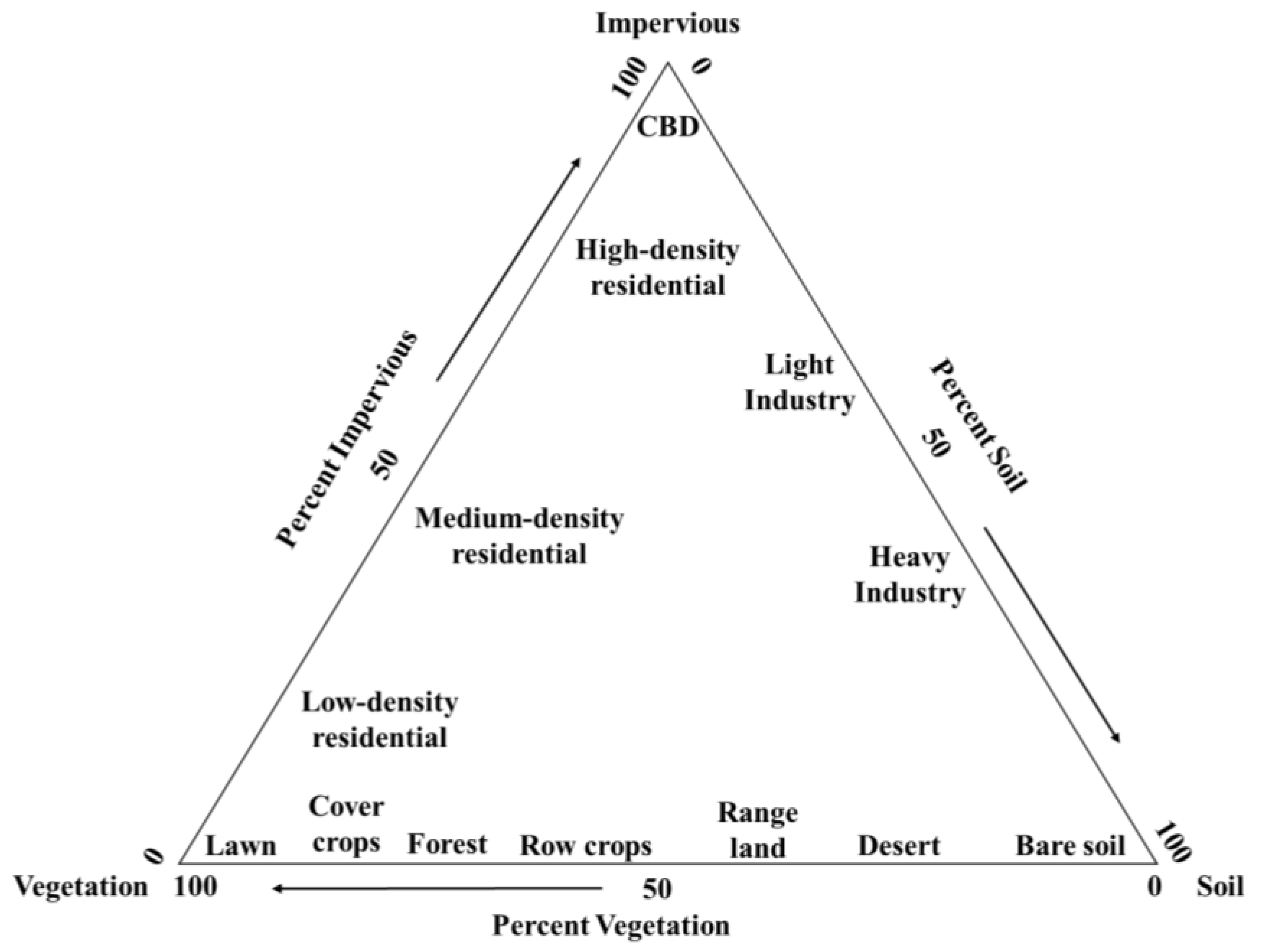
22]. Hence, the inclusion of ISC can potentially increase the accuracy of modeling the USES. Based on the Vegetation-Impervious surface-Soil (V-I-S) model [23], the percentage of each of the three fractions of impervious, vegetation, and soil covers in a pixel indicates the difference in the surface characteristics of different urban land cover/uses. This model assumes that land cover in urban environments is a linear combination of three components.
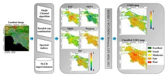
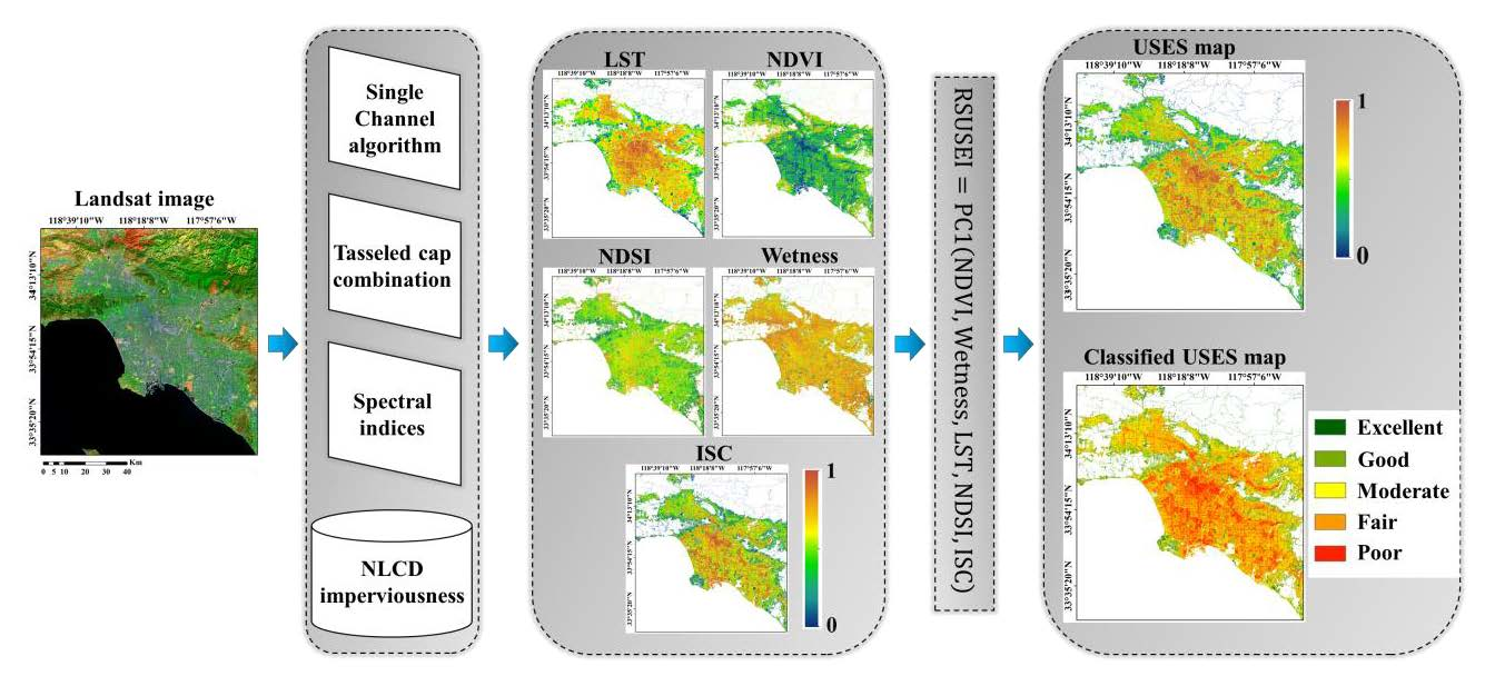
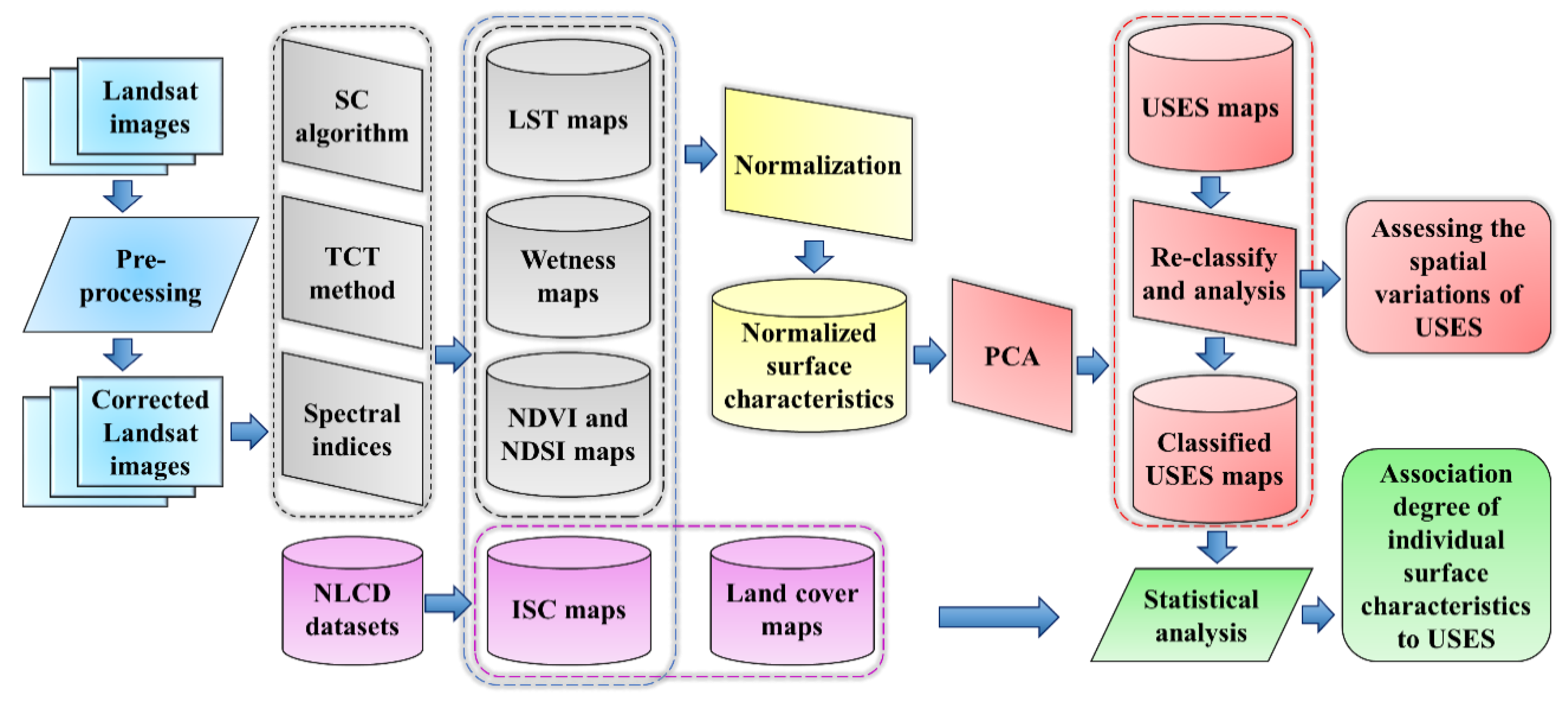
The objective of this study is to present a new analytical framework for assessing the Remotely Sensed Urban Surface Ecological index (RSUSEI) by integration of surface greenness, moisture, dryness, heat, and imperviousness using Principal Components Analysis (PCA). Based on the V-I-S model, this study intends to assess USES and compare six cities of the U.S.A including Minneapolis, Dallas, Phoenix, Los Angeles, Chicago, and Seattle which have distinct geographical, geological, climatic, environmental, and surface biophysical conditions.

2. Study Area

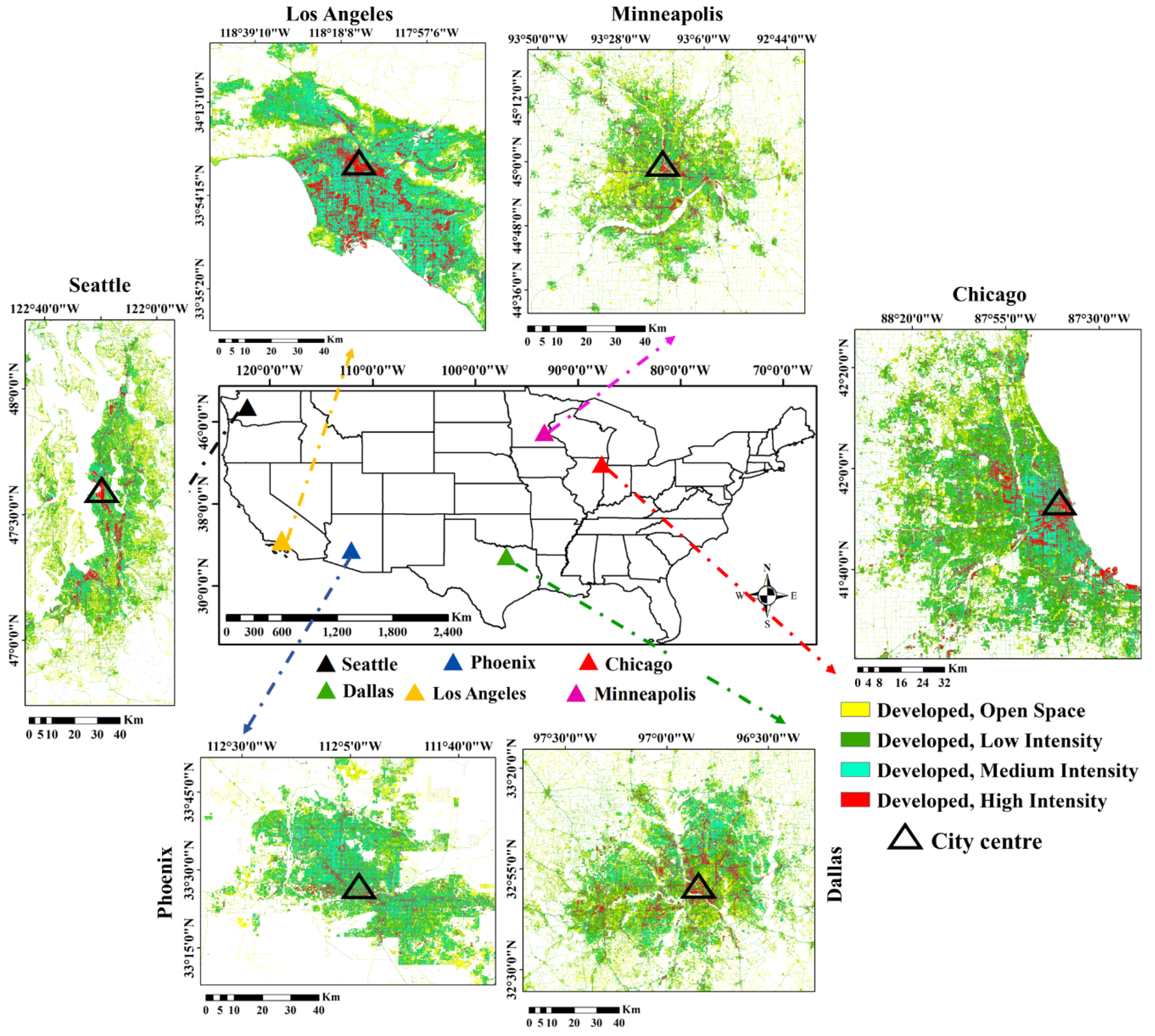
The new analytical framework for assessing the SES is tested in urban environments comprising the cities of Minneapolis, Dallas, Phoenix, Los Angeles, Chicago, and Seattle (Figure 1). To select these cities, various criteria such as (1) geographical conditions, (2) climatic conditions, (3) surface characteristics, (4) density of population, and (5) physical size of the cities were considered. These cities possess different geographical, climatic, environmental, and biophysical conditions. Based on the Köppen climate classification, the selected cities have various climate types: humid continental (Dfa—Minneapolis, Chicago), tropical and subtropical desert (Bwh—Phoenix), dry-summer subtropical (Csa—Los Angeles; Csb—Seattle), or humid subtropical (Cfa—Dallas). Thus, the spatial variability of the surface cover and biophysical characteristics of these cities are different and heterogeneous.
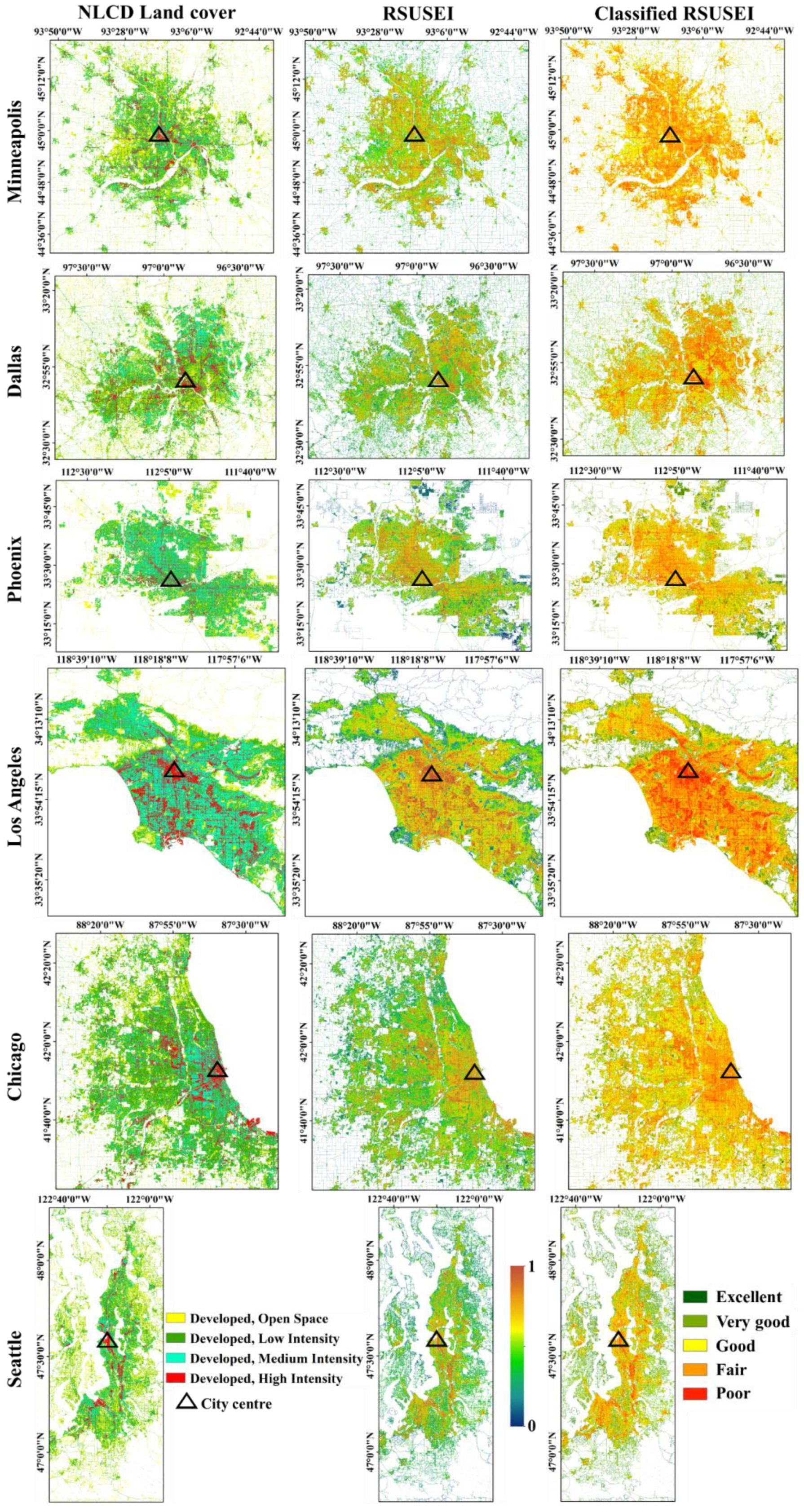
For the selected cities in the U.S.A, the area and percentage of each land cover are different (Figure 1 and Table 1). The highest area of land cover in Minneapolis, Dallas, Phoenix, Los Angeles, Chicago, and Seattle cities is related to “Developed, Open Space”, “Developed, Low Intensity”, “Developed, Low Intensity”, “Developed, Medium Intensity”, “Developed, Low Intensity”, and “Developed, Low Intensity”, respectively. Among the cities, the highest percentage of “Developed, Open Space”, “Developed, Low Intensity”, “Developed, Medium Intensity”, and “Developed, High Intensity” lands is found in Minneapolis (36.0%), Chicago (45.5%), Los Angeles (44.6%), and Los Angeles (16.3%), respectively.

3. Data and Methods

3.1. Data

A leaf-on season of Landsat 8 image for each city was downloaded for use from the U.S.A Geological Survey (USGS) website (http://www.usgs.gov), including Minneapolis (date: 8 September, 2016), Dallas (8 September, 2016), Phoenix (14 September, 2016), Los Angeles (26 September, 2016), Chicago (12 September, 2016), and Seattle (13 September, 2016). Due to the spatial, temporal, spectral, and radiometric resolution, Landsat images are suitable for modeling and monitoring environmental and ecological conditions [24,25,26]. These images are georeferenced with the number of rows and paths available. The spatial resolution of Landsat 8 reflective and thermal bands are 30 and 100 m, respectively. Resampled thermal infrared bands based on the Cubic method with a spatial resolution of 30 m are also available on the USGS website. Due to the climatic and seasonal effects on USES, leaf-on clear-sky images were selected for this study. Furthermore, the Moderate Resolution Imaging Spectroradiometer (MODIS) water vapor product (MOD07) with a spatial resolution of 5000 m was used to calculate Land Surface Temperature (LST) from the Landsat images. This product contains the following features: (1) total-ozone burden, (2) atmospheric stability, (3) temperature and moisture profiles, (4) and atmospheric water vapor. In addition, datasets from the National Land Cover Database (NLCD), including land cover and imperviousness for 2016 were used. The imperviousness data were utilized to represent surface biophysical characteristics, while the land cover data to evaluate the impact of land cover on USES. The NLCD land cover and imperviousness datasets with 30 m spatial resolutions for the U.S.A prepared for different years using Landsat time-series images [27,28] are available from USGS at the https://www.mrlc.gov/data website.

3.2. Methods

Firstly, Landsat imagery was preprocessed. In the second step, the Single Channel (SC) algorithm, the Tasseled cap transformation, spectral indices, and the NLCD imperviousness data product were used to derive surface biophysical characteristics, which include NDVI, Wetness, NDSI, LST, and ISC for the selected cities. Next, USES of the selected cities were modeled by the combination of surface biophysical characteristics data using PCA. Then, the spatial variations of USES across different selected cities were evaluated and compared to each other. Finally, the association degree of each surface biophysical characteristic on USES was investigated based on statistical analysis (Figure 2).

3.2.1. Landsat Image Preprocessing and Surface Characteristics Modeling

The Fast Line-of-sight Atmospheric Analysis of Spectral Hypercubes (FLAASH) model was applied for the atmospheric correction of Landsat images. This model uses parameters such as satellite overpass time, sensor altitude, geographic location, atmospheric model of the region, and the solar elevation and zenith angels [29,30].
The spectral indices used in this study included NDVI (greenness), Wetness (moisture), NDSI (dryness), and LST (heat), which are shown in Table 2.
Land cover and imperviousness maps of the selected cities were obtained from NLCD in 2016. Land cover maps of the urban areas based on this dataset included classes of “Developed, Open Space”, “Developed, Low Intensity”, “Developed, Medium Intensity”, and “Developed, High Intensity”. The percentage urban impervious surface was resolved in 1% increments from 0 to 100 for areas identified as urban, in the land cover layer of the database.

3.2.2. Remotely Sensed Urban Surface Ecological Index (RSUSEI)

In this study, RSUSEI was developed to assess the USES. Urban surfaces were assumed to consist of three fractions of impervious, vegetation, and soil covers. Based on the V-I-S model, the percentage of each of these surface covers in a pixel indicated the difference in the surface characteristics of different urban land cover/uses (Figure 3). This model assumes that land cover in urban environments is a linear combination of three components [23]. Therefore, to model accurately the USES and to assess the SES of different land covers in urban environments, it is important to consider the biophysical characteristics related to the fractions of impervious, vegetation, and soil cover.
Surface greenness, dryness, moisture, heat, and imperviousness are the biophysical characteristics that were utilized to describe these component surfaces and are integrated for analysis of USES. It can be represented as Equation (1):
USES = f ( Greenness ,   Dryness ,   Moisture ,   Heat ,   Imperviousness )
However, these environmental and surface biophysical parameters may be correlated with each other in a region. The use of PCA can be very useful to solve the collinearity between the predictive variables in the model of USES. To reduce the effect of climatic and meteorological conditions on the results of the RSUSEI, standardized values of LST (heat), NDVI (greenness), NDSI (dryness), Wetness (moisture), and ISC (imperviousness) indices (between 0 and 1) were computed [36]. Then, the PCA method was employed to combine the five indices for assessing the USES. Finally, the PC1 was selected to represent USES in the urban environments. RSUSEI can then be modeled conceptually based on Equation (2).
RSUSEI = PC 1 ( NDVI ,   Wetness ,   LST ,   NDSI ,   ISC )
RSUSEI values were normalized between 0 and 1. The maximum value was related to the worst (highest LST, ISC, and NDSI, but lowest NDVI and Wetness) and the minimum value to the best USES (lowest LST, ISC, and NDSI, but highest NDVI and Wetness). To analyze and evaluate the spatial variations of USES, the normalized values of RSUSEI were grouped into five classes: Excellent (0–0.2), Very Good (0.2–0.4), Good (0.4–0.6), Fair (0.6–0.8), and Poor (0.8–1) [4,5,6]. The mean and Standard Deviation (SD) values of RSUSEI were calculated and the area of USES classes were mapped for each city. Additionally, the Eigenvalues of the five main components of PCA for each city were calculated.

3.2.3. Association Degree of Individual Surface Characteristics to USES

To calculate and assess the association degree of each surface characteristic to USES, the mean value of RSUSEI was calculated by the NLCD land cover class for the six selected cities. The correlation coefficient (r) between RSUSEI and each biophysical variable, i.e., LST, NDVI, NDSI, and Wetness, is calculated for each city. In addition, the mean RSUSEI value for different ISC percentage ranges (1 to 100) was calculated and then the r between the mean RSUSEI values and the percentage of ISC was calculated for each city.

4. Results

4.1. Spatial Distribution of Surface Characteristics

Figure 4 shows maps of surface biophysical characteristics including Normalized LST (nLST), Normalized NDVI (nNDVI), Normalized NDSI (nNDSI), and Normalized Wetness (nWetness) in the selected cities. The spatial pattern was heterogeneous. A large proportion of the central parts of all these selected cities included developed lands (ISC > 50%). The suburbs of Minneapolis, Dallas, Chicago, and Seattle included land covers with a high percentage of vegetation cover, while in Phoenix and Los Angeles there were bare lands with dry surfaces. In all cities, the values of nLST and nNDSI in the central parts of the cities were higher than the other parts, while nNDVI values were lower. In addition, the spatial distribution of ISC values in these cities was heterogeneous. Areas with developed and nature lands had the highest and lowest values of ISC, respectively.
The mean and SD values of nLST, nNDVI, nNDSI, nWetness, and nISC in the selected cities were different. The difference in the mean values of these spectral indices indicated the difference in the surface biophysical characteristics of these cities. High SD values of these spectral indices indicated a higher degree of spatial variability of the surface biophysical characteristics. The correlation coefficient (r) between the mean values of nLST and nNDVI, nNDSI, nWetness, and nISC for these cities were −0.92, 0.95, −0.22, and 0.88, respectively, which indicated a strong correlation between different surface biophysical characteristics, except Wetness. The statistical significance of these correlations were confirmed at 95% confidence level. Cities with high mean values of nLST and nNDSI tended to have low mean values of nNDVI and vice versa (Table 3). By reducing surface vegetation, the amount of evapotranspiration from the surface decreased, leading to an increase in surface heat and dryness. In addition, a higher value of ISC caused an increase in the value of LST (heat) and NDSI (dryness) and a decrease in the value of NDVI (greenness) and Wetness (moisture).
The spatial distribution of surface biophysical characteristic differences can be caused by the differences in the spatial variability of land covers [19,37,38,39,40]. Table 4 shows that surface biophysical characteristics including nLST, nNDVI, nNDSI, nWetness, and nISC were different for each land cover. Anthropogenic activities reduce natural surface covers and affect surface characteristics including surface reflection, change in the material’s thermal capacity, conductivity, diffusion, albedo, and evapotranspiration [19,37,41,42,43]. For the selected cities, the highest (lowest) mean values of nLST, nNDSI, and nISC and the lowest (highest) values of nNDVI and nWetness were related to Developed, High Intensity (Developed, Open Space). Therefore, due to the spatial variability of land covers, the spatial variability of surface biophysical characteristics in the selected cities were different.

4.2. Spatial Distribution of USES

The spatial distribution of USES of the selected cities was heterogeneous (Figure 5). A visual survey of the RSUSEI maps shows that Chicago and Los Angeles had higher RSUSEI values than Minneapolis, Dallas, Phoenix, and Seattle. Areas with high values of RSUSEI (red color) had a lower quality of USES, which had high heat (LST), imperviousness (ISC) dryness (NDSI), greenness (NDVI), and moisture (Wetness) values, and vice versa. Figure 6 shows the mean value of RSUSEI for Minneapolis, Dallas, Phoenix, Los Angeles, Chicago, and Seattle to be 0.58, 0.54, 0.47, 0.63, 0.50, and 0.44, respectively. The difference in the mean value of RSUSEI between the cities indicated a significant difference in their USES. The best and worst USES were Seattle and Los Angeles, respectively. The SD values of RSUSEI for Minneapolis (0.16), Dallas (0.17), Phoenix (0.19), Los Angeles (0.21), Chicago (0.17), and Seattle (0.19) cities were high. These values indicated the high spatial variability of the USES within each selected city. Overall, the SD values of the different cities were very similar. The highest and lowest spatial variations of USES were observed in Minneapolis and Seattle, respectively.
The spatial distribution of the RSUSEI classes further revealed the spatial variability of USES across the selected cities (Figure 7). Overall, the majority of the land in the selected cities possessed the USES class from Very Good to Fair. The highest percentage of USES class for Minneapolis, Dallas, Phoenix, Chicago, and Seattle cities was Good and for Los Angeles city was Fair. The Poor class of USES had better spatial coverage of 5% to 14%, compared to that of the Excellent class from 1% to 6%. In addition, the highest percentage of Excellent, Very Good, Good, Fair, and Poor classes of USES was observed in Los Angeles, Seattle, Chicago, Minneapolis, and Los Angeles, respectively (Figure 7). The spatial heterogeneity of surface biophysical characteristics and anthropogenic activities caused differences in USES among the cities and within each city.
It is worth noting that the Eigenvalues of the PC1 in RSUSEI modeling for the Minneapolis, Dallas, Phoenix, Los Angeles, Chicago, and Seattle cities were 0.33, 0.34, 0.40, 0.39, 0.29, and 0.37, respectively. For all selected cities, PC1 included more than 93% of the main surface information including greenness, moisture, dryness, heat, and imperviousness. Therefore, using PC1 in RSUSEI can well represent the spatial heterogeneity is the USES.

4.3. Association Degree of Surface Biophysical Parameters on the USES Modeling

The mean value of RSUSEI varied across different land covers in the selected cities (Table 5). The mean values of RSUSEI in “Developed, Open Space”, “Developed, Low Intensity”, “Developed, Medium Intensity”, and “Developed, High Intensity” lands were 0.35, 0.49, 0.63, and 0.76, respectively (Table 6). In general, “Developed, high intensity” and “Developed, Open Space” lands detected the highest and lowest RSUSEI values in these cities, respectively. This result suggests the effectiveness of RSUSEI to separate USES by land cover.
Areas with high surface heat (LST), imperviousness (ISC), dryness (NDSI), low surface vegetation density (NDVI), and moisture (Wetness) exhibited poor USES. The locations of these areas corresponded to “Developed, High Intensity” lands (Figure 5). By contrast, “Developed, Open Space” lands possessed the best USES (Table 4), which discovered low values of LST and NDSI and high values of NDVI and Wetness. Mixed pixels in warm and dry cities tended to include built-up lands and lands with low vegetation cover and low moisture content. Due to the high values of RSUSEI for lands with low vegetation density and low moisture content, these cities discovered poor USES. On the other hand, mixed pixels in humid cities were associated with high vegetation density and surface moisture. Since there were low values of RSUSEI for lands with high vegetation density and high surface moisture, these cities experienced poor USES. These findings suggest that RSUSEI holds an excellent ability to differentiate between USES of different land covers (Figure 4 and Table 5).
The association degree of nLST, nNDVI, nNDSI, and nWetness in RSUSEI in the selected cities varied. The mean r between nLST, nNDVI, nNDSI, and nWetness and RSUSEI was 0.47, −0.31, 0.17, and −0.27, respectively (Table 6). The statistical significance of these correlations were confirmed at 95% confidence level. In modeling the USES, the association degree of nLST was found to be higher than nNDVI, nNDSI, and nWetness. For the RSUSEI modeling in Los Angeles, Chicago, and Seattle cities, the association degree of nNDVI appeared higher than nNDSI and nWetness. In contrast, in Minneapolis and Dallas, the association degree of nWetness was higher than nNDVI and nNDSI.
The correlation coefficient between the mean value of RSUSEI and the mean value of NLCD imperviousness percentage was 0.93 for all cities, but it varied within cities. Minneapolis, Dallas, Phoenix, Los Angeles, Chicago, and Seattle yielded an r value of 0.90, 0.99, 0.99, 0.99, 0.98, and 0.98, respectively (Table 6). The statistical significance of these correlations are confirmed at 95% confidence level. These values indicated a positive strong correlation between ISC and RSUSEI. The spatial variation patterns of RSUSEI and NLCD imperviousness were similar to each other (Figure 5). The RSUSEI value increased with increasing the percentage of impervious surface. In the USES modeling, the association degree of ISC was highest among all the surface parameters used in this study.

5. Discussion

The SES in urban environments is a function of the surface biophysical, biochemical, and biological properties. Recent studies have used the data of surface greenness, moisture, dryness, and heat for SES modeling [4,6,7]. However, many processes in the urban environments are subject to the impact of surface imperviousness [23,44,45,46]. ISC has a clear physical meaning in land surface composition, suitable for distinguishing the characteristics of different types of land use and land cover in the urban environments, and is associated with changes in the characteristics of surface greenness, moisture, dryness, and heat [19,20,22,45]. This study shows that the association degree of imperviousness is higher than surface heat, greenness, dryness, and moisture. Therefore, considering surface imperviousness information in USES modeling is very necessary. Other studies have also shown that surface imperviousness affected the SES [4,47,48]. For many cities around the world, surface imperviousness data are available with functional spatial resolution for urban modeling. In this study, five components including surface greenness, moisture, dryness, heat, and imperviousness are considered for RSUSEI development. Results showed that RSUSEI is highly capable in the modeling of the USES spatial heterogeneity in cities with different geographical, climatic, environmental, and biophysical conditions. This index has a high capacity to differentiate between USES of different land covers. Assessment and modeling of USES are crucial in sustainability assessment in support of achieving sustainable development goals such as sustainable cities and communities [8]. Hence, RSUSEI can be used for assessing urban sustainability over space and time.

6. Conclusions

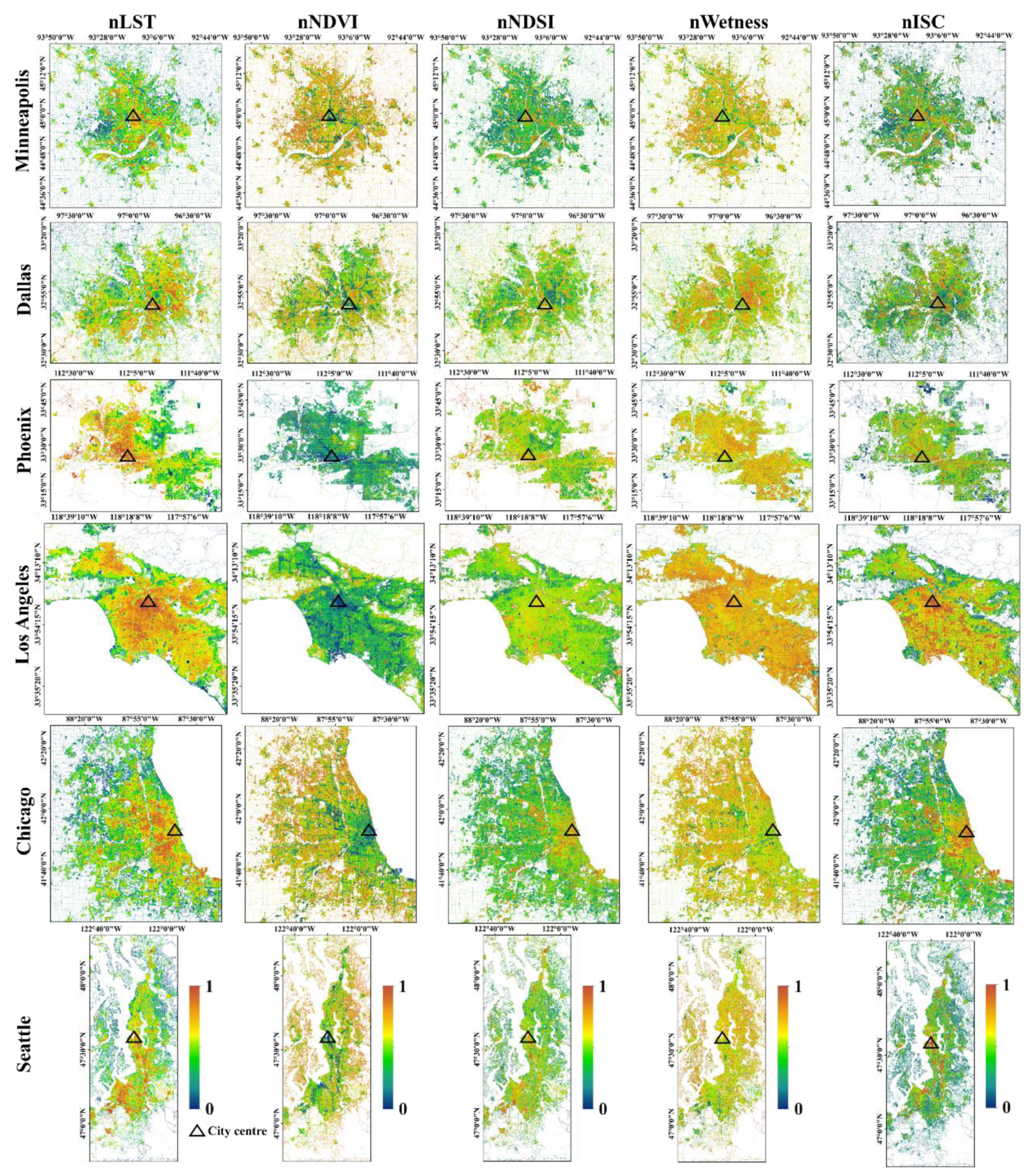
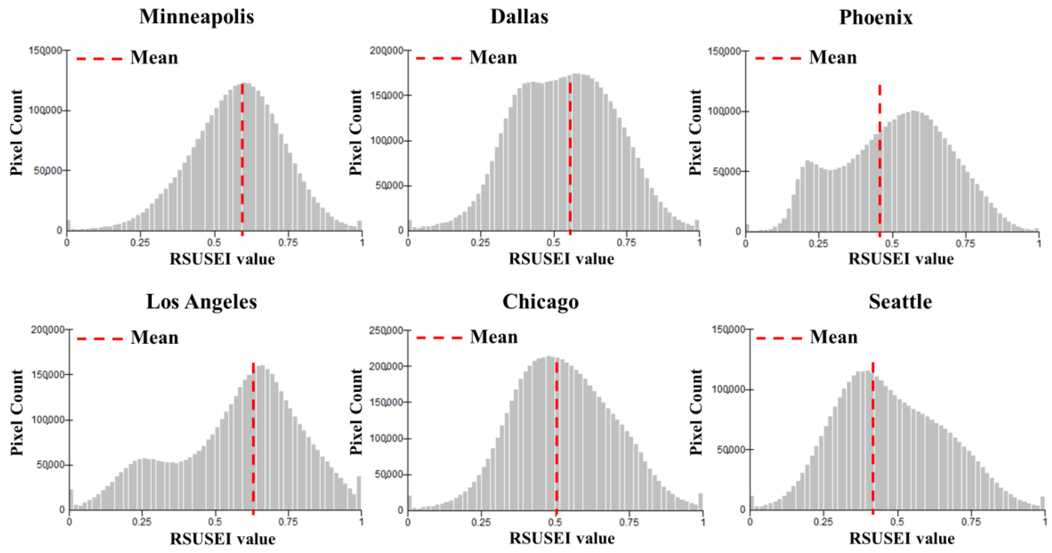
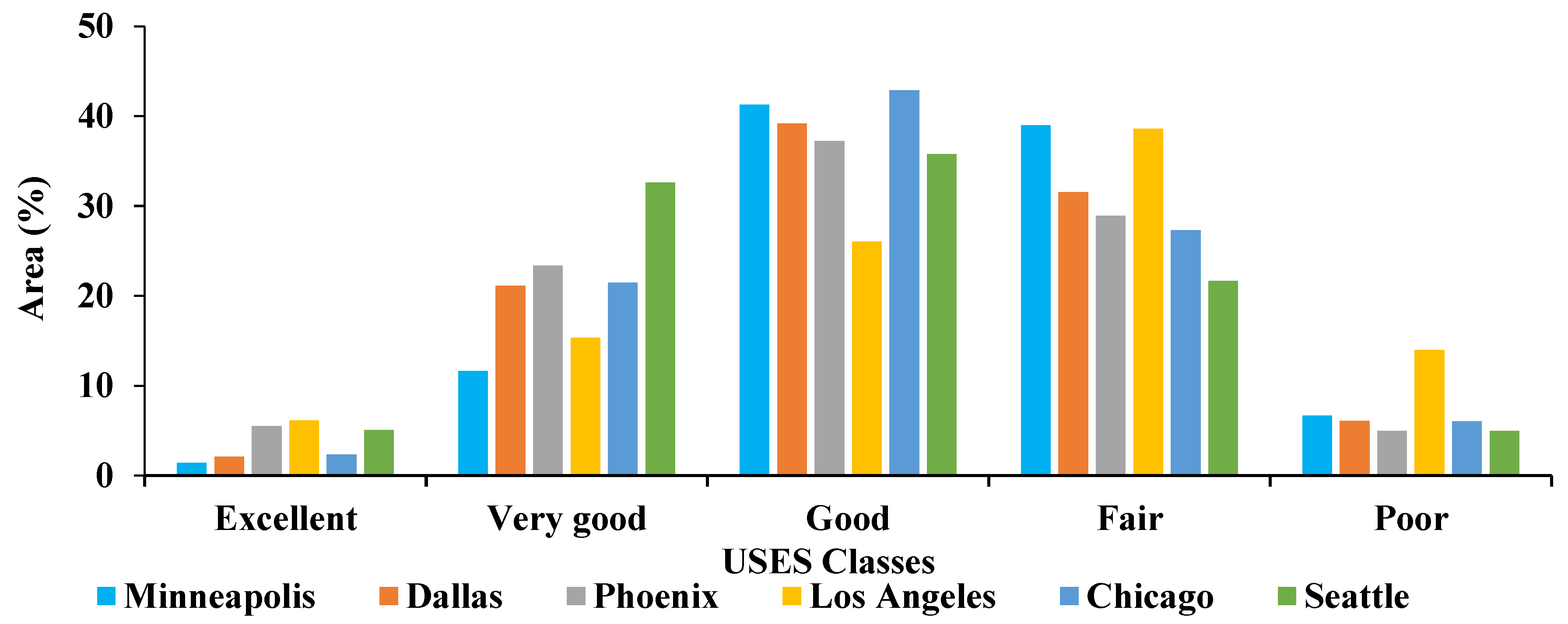
In this study, an analytical framework is proposed for assessing the SES in urban environments and tested in six selected cities in the U.S.A, i.e., Minneapolis, Dallas, Phoenix, Los Angeles, Chicago, and Seattle. This analytical framework is centered on a new index, Remotely Sensed Urban Surface Ecological index (RSUSEI), which integrated satellite derived information on the greenness, moisture, dryness, heat, and imperviousness in a city. The results showed that the spatial distribution of USES varied with the cities and land cover types. In general, land covers with low vegetation density and moisture, and high heat, imperviousness, and dryness exhibit high RSUSEI values and poor USES, and vice versa. The USES in arid regions, such as Los Angeles, are found to be worse than the USES in humid regions, such as Seattle. The association degree of ISC is higher than nLST, nNDVI, nNDSI, and nWetness in the RSUSEI modeling. An increase in surface imperviousness reduces surface vegetation density and moisture while increasing surface dryness and heat degree, thereby worsening USES. Our results show that RSUSEI has a high capability in revealing the differences in USES within and between cities with different geographical, climatic, environmental, and surface conditions. Due to the functional spatial resolution and continuity of Landsat imagery, the results of this study can be very useful in USES modeling in urban environments with different biophysical, geographical, and climatic conditions. In addition, the availability of NLCD data products in the U.S.A is highly beneficial for USES assessment, monitoring, and modeling. RSUSEI can be used for assessing urban sustainability over space and time. It is suggested that in future studies, the efficiency of disaggregation models in improving the spatial resolution of USES maps should be considered. It is also useful to compare the performance of different spectral indices in surface imperviousness modeling to assess USES. In addition, RSUSEI can be used as a time series to monitor and model the long-term changes in a region and to quantify the impact of anthropogenic activities on USES.

Author Contributions

M.K.F. and S.F. conceived and designed the research of, and wrote, the first draft; Q.W. re-designed the research, and revised and edited the paper; M.K. and S.K.A. provided comments. All authors contributed to, and approved, the final manuscript. All authors have read and agreed to the published version of the manuscript.

Funding

This research received no external funding.

Conflicts of Interest

The authors declare no conflict of interest.

References

  1. Reza, M.I.H.; Abdullah, S.A. Regional Index of Ecological Integrity: A need for sustainable management of natural resources. Ecol. Indic. 2011, 11, 220–229. [Google Scholar] [CrossRef]
  2. Frohn, R.C.; Lopez, R.D. Remote Sensing for Landscape Ecology: New Metric Indicators: Monitoring, Modeling, and Assessment of Ecosystems; CRC Press: Boca Raton, FL, USA, 2017. [Google Scholar]
  3. Wu, Z.; Zhang, Y. Water Bodies’ Cooling Effects on Urban Land Daytime Surface Temperature: Ecosystem Service Reducing Heat Island Effect. Sustainability 2019, 11, 787. [Google Scholar] [CrossRef] [Green Version]
  4. Xu, H.; Wang, M.; Shi, T.; Guan, H.; Fang, C.; Lin, Z. Prediction of ecological effects of potential population and impervious surface increases using a remote sensing based ecological index (RSEI). Ecol. Indic. 2018, 93, 730–740. [Google Scholar] [CrossRef]
  5. Xu, H.; Wang, Y.; Guan, H.; Shi, T.; Hu, X. Detecting Ecological Changes with a Remote Sensing Based Ecological Index (RSEI) Produced Time Series and Change Vector Analysis. Remote Sens. 2019, 11, 2345. [Google Scholar] [CrossRef] [Green Version]
  6. Hu, X.; Xu, H. A new remote sensing index for assessing the spatial heterogeneity in urban ecological quality: A case from Fuzhou City, China. Ecol. Indic. 2018, 89, 11–21. [Google Scholar] [CrossRef]
  7. Zhu, X.; Wang, X.; Yan, D.; Liu, Z.; Zhou, Y. Analysis of remotely-sensed ecological indexes’ influence on urban thermal environment dynamic using an integrated ecological index: A case study of Xi’an, China. Int. J. Remote Sens. 2019, 40, 3421–3447. [Google Scholar] [CrossRef]
  8. Estoque, R.C. A Review of the Sustainability Concept and the State of SDG Monitoring Using Remote Sensing. Remote Sens. 2020, 12, 1770. [Google Scholar] [CrossRef]
  9. Lin, T.; Ge, R.; Huang, J.; Zhao, Q.; Lin, J.; Huang, N.; Zhang, G.; Li, X.; Ye, H.; Yin, K. A quantitative method to assess the ecological indicator system’s effectiveness: A case study of the Ecological Province Construction Indicators of China. Ecol. Indic. 2016, 62, 95–100. [Google Scholar] [CrossRef]
  10. Pettorelli, N.; Vik, J.O.; Mysterud, A.; Gaillard, J.-M.; Tucker, C.J.; Stenseth, N.C. Using the satellite-derived NDVI to assess ecological responses to environmental change. Trends Ecol. Evol. 2005, 20, 503–510. [Google Scholar] [CrossRef] [PubMed]
  11. Willis, K.S. Remote sensing change detection for ecological monitoring in United States protected areas. Biol. Conserv. 2015, 182, 233–242. [Google Scholar] [CrossRef]
  12. Cohen, W.B.; Goward, S.N. Landsat’s role in ecological applications of remote sensing. Bioscience 2004, 54, 535–545. [Google Scholar] [CrossRef]
  13. Sun, Z.; Chang, N.-B.; Opp, C. Using SPOT-VGT NDVI as a successive ecological indicator for understanding the environmental implications in the Tarim River Basin, China. J. Appl. Remote Sens. 2010, 4, 043554. [Google Scholar]
  14. Estoque, R.C.; Murayama, Y. Monitoring surface urban heat island formation in a tropical mountain city using Landsat data (1987–2015). ISPRS J. Photogramm. 2017, 133, 18–29. [Google Scholar] [CrossRef]
  15. He, C.; Gao, B.; Huang, Q.; Ma, Q.; Dou, Y. Environmental degradation in the urban areas of China: Evidence from multi-source remote sensing data. Remote Sens. Environ. 2017, 193, 65–75. [Google Scholar] [CrossRef]
  16. Fu, P.; Xie, Y.; Weng, Q.; Myint, S.; Meacham-Hensold, K.; Bernacchi, C. A physical model-based method for retrieving urban land surface temperatures under cloudy conditions. Remote Sens. Environ. 2019, 230, 111191. [Google Scholar] [CrossRef]
  17. Fu, Y.; Li, J.; Weng, Q.; Zheng, Q.; Li, L.; Dai, S.; Guo, B. Characterizing the spatial pattern of annual urban growth by using time series Landsat imagery. Sci. Total Environ. 2019, 666, 274–284. [Google Scholar] [CrossRef]
  18. King, R.S.; Baker, M.E. Considerations for analyzing ecological community thresholds in response to anthropogenic environmental gradients. J. N. Am. Benthol. Soc. 2010, 29, 998–1008. [Google Scholar] [CrossRef] [Green Version]
  19. Firozjaei, M.K.; Weng, Q.; Zhao, C.; Kiavarz, M.; Lu, L.; Alavipanah, S.K. Surface anthropogenic heat islands in six megacities: An assessment based on a triple-source surface energy balance model. Remote Sens. Environ. 2020, 242, 111751. [Google Scholar] [CrossRef]
  20. Weng, Q.; Lu, D.; Liang, B. Urban surface biophysical descriptors and land surface temperature variations. Photogramm. Eng. Remote Sens. 2006, 72, 1275–1286. [Google Scholar] [CrossRef] [Green Version]
  21. Weng, Q.; Liu, H.; Liang, B.; Lu, D. The spatial variations of urban land surface temperatures: Pertinent factors, zoning effect, and seasonal variability. IEEE J. Sel. Top. Appl. Earth Obs. Remote Sens. 2008, 1, 154–166. [Google Scholar] [CrossRef]
  22. Lu, D.; Weng, Q. Extraction of urban impervious surfaces from an IKONOS image. Int. J. Remote Sens. 2009, 30, 1297–1311. [Google Scholar] [CrossRef]
  23. Ridd, M.K. Exploring a VIS (vegetation-impervious surface-soil) model for urban ecosystem analysis through remote sensing: Comparative anatomy for cities. Int. J. Remote Sens. 1995, 16, 2165–2185. [Google Scholar] [CrossRef]
  24. Firozjaei, M.K.; Sedighi, A.; Kiavarz, M.; Qureshi, S.; Haase, D.; Alavipanah, S.K. Automated Built-Up Extraction Index: A New Technique for Mapping Surface Built-Up Areas Using LANDSAT 8 OLI Imagery. Remote Sens. 2019, 11, 1966. [Google Scholar] [CrossRef] [Green Version]
  25. Amiri, R.; Weng, Q.; Alimohammadi, A.; Alavipanah, S.K. Spatial–temporal dynamics of land surface temperature in relation to fractional vegetation cover and land use/cover in the Tabriz urban area, Iran. Remote Sens. Environ. 2009, 113, 2606–2617. [Google Scholar] [CrossRef]
  26. Haashemi, S.; Weng, Q.; Darvishi, A.; Alavipanah, S.K. Seasonal variations of the surface urban heat island in a semi-arid city. Remote Sens. 2016, 8, 352. [Google Scholar] [CrossRef] [Green Version]
  27. Xian, G.; Homer, C.; Demitz, J.; Fry, J.; Hossain, N. Change of impervious surface area between 2001 and 2006 in the conterminous United States. Photogramm. Eng. Remote Sens. 2011, 77, 758–762. [Google Scholar]
  28. Yang, L.; Huang, C.; Homer, C.G.; Wylie, B.K.; Coan, M.J. An approach for mapping large-area impervious surfaces: Synergistic use of Landsat-7 ETM+ and high spatial resolution imagery. Can. J. Remote Sens. 2003, 29, 230–240. [Google Scholar] [CrossRef]
  29. Berk, A.; Conforti, P.; Kennett, R.; Perkins, T.; Hawes, F.; van den Bosch, J. MODTRAN® 6: A major upgrade of the MODTRAN® radiative transfer code. In Proceedings of the 2014 6th Workshop on Hyperspectral Image and Signal Processing: Evolution in Remote Sensing (WHISPERS), Lausanne, Switzerland, 24–27 June 2014; pp. 1–4. [Google Scholar]
  30. Firozjaei, M.K.; Kiavarz, M.; Nematollahi, O.; Karimpour Reihan, M.; Alavipanah, S.K. An evaluation of energy balance parameters, and the relations between topographical and biophysical characteristics using the mountainous surface energy balance algorithm for land (SEBAL). Int. J. Remote Sens. 2019, 40, 1–31. [Google Scholar] [CrossRef]
  31. Tucker, C.J. Red and photographic infrared linear combinations for monitoring vegetation. Remote Sens. Environ. 1979, 8, 127–150. [Google Scholar] [CrossRef] [Green Version]
  32. Baig, M.H.A.; Zhang, L.; Shuai, T.; Tong, Q. Derivation of a tasselled cap transformation based on Landsat 8 at-satellite reflectance. Remote Sens. Lett. 2014, 5, 423–431. [Google Scholar] [CrossRef]
  33. Mijani, N.; Alavipanah, S.K.; Hamzeh, S.; Firozjaei, M.K.; Arsanjani, J.J. Modeling thermal comfort in different condition of mind using satellite images: An Ordered Weighted Averaging approach and a case study. Ecol. Indic. 2019, 104, 1–12. [Google Scholar] [CrossRef]
  34. Zhao, H.; Chen, X. Use of normalized difference bareness index in quickly mapping bare areas from TM/ETM+. In Proceedings of the International geoscience and remote sensing symposium, Seoul, Korea, 25–29 July 2005; p. 1666. [Google Scholar]
  35. Jiménez-Muñoz, J.C.; Sobrino, J.A.; Skoković, D.; Mattar, C.; Cristóbal, J. Land surface temperature retrieval methods from Landsat-8 thermal infrared sensor data. IEEE Geosci. Remote Sens. Lett. 2014, 11, 1840–1843. [Google Scholar] [CrossRef]
  36. Firozjaei, M.K.; Alavipanah, S.K.; Liu, H.; Sedighi, A.; Mijani, N.; Kiavarz, M.; Weng, Q. A PCA–OLS Model for Assessing the Impact of Surface Biophysical Parameters on Land Surface Temperature Variations. Remote Sens. 2019, 11, 2094. [Google Scholar] [CrossRef] [Green Version]
  37. Fu, P.; Weng, Q. A time series analysis of urbanization induced land use and land cover change and its impact on land surface temperature with Landsat imagery. Remote Sens. Environ. 2016, 175, 205–214. [Google Scholar] [CrossRef]
  38. Firozjaei, M.K.; Fathololoumi, S.; Kiavarz, M.; Arsanjani, J.J.; Alavipanah, S.K. Modelling surface heat island intensity according to differences of biophysical characteristics: A case study of Amol city, Iran. Ecol. Indic. 2020, 109, 105816. [Google Scholar] [CrossRef]
  39. Firozjaei, M.K.; Kiavarz, M.; Alavipanah, S.K.; Lakes, T.; Qureshi, S. Monitoring and forecasting heat island intensity through multi-temporal image analysis and cellular automata-Markov chain modelling: A case of Babol city, Iran. Ecol. Indic. 2018, 91, 155–170. [Google Scholar] [CrossRef]
  40. Karimi, F.M.; Kiavarz, M.M.; Alavi, P.S.K. Monitoring and predicting spatial-temporal changes heat island in babol city due to urban sprawl and land use changes. Eng. J. Geospat. Inf. Technol. 2017, 5, 123–151. [Google Scholar]
  41. Liu, H.; Weng, Q. Seasonal variations in the relationship between landscape pattern and land surface temperature in Indianapolis, USA. Environ. Monit. Assess. 2008, 144, 199–219. [Google Scholar] [CrossRef]
  42. Lu, D.; Weng, Q. Spectral mixture analysis of ASTER images for examining the relationship between urban thermal features and biophysical descriptors in Indianapolis, Indiana, USA. Remote Sens. Environ. 2006, 104, 157–167. [Google Scholar] [CrossRef]
  43. Weng, Q.; Hu, X.; Quattrochi, D.A.; Liu, H. Assessing intra-urban surface energy fluxes using remotely sensed ASTER imagery and routine meteorological data: A case study in Indianapolis, USA. IEEE J. Sel. Top. Appl. Earth Obs. Remote Sens. 2014, 7, 4046–4057. [Google Scholar] [CrossRef]
  44. Weng, Q. Remote sensing of impervious surfaces in the urban areas: Requirements, methods, and trends. Remote Sens. Environ. 2012, 117, 34–49. [Google Scholar] [CrossRef]
  45. Weng, Q.; Lu, D. A sub-pixel analysis of urbanization effect on land surface temperature and its interplay with impervious surface and vegetation coverage in Indianapolis, United States. Int. J. Appl. Earth Obs. 2008, 10, 68–83. [Google Scholar] [CrossRef]
  46. Weng, Q.; Rajasekar, U.; Hu, X. Modeling urban heat islands and their relationship with impervious surface and vegetation abundance by using ASTER images. IEEE Trans. Geosci. Remote Sens. 2011, 49, 4080–4089. [Google Scholar] [CrossRef]
  47. Wickham, J.; Wade, T.; Norton, D. Spatial patterns of watershed impervious cover relative to stream location. Ecol. Indic. 2014, 40, 109–116. [Google Scholar] [CrossRef]
  48. Beck, S.M.; McHale, M.R.; Hess, G.R. Beyond impervious: Urban land-cover pattern variation and implications for watershed management. Environ. Manag. 2016, 58, 15–30. [Google Scholar] [CrossRef] [PubMed]
Figure 1. Geographical location of selected cities including Minneapolis, Dallas, Phoenix, Los Angeles, Chicago, and Seattle in the U.S.A and land cover maps of each selected cities.
Remotesensing 12 02029 g001
Figure 2. The flowchart of the analytical framework. SC: Single Channel, TCT: Tasseled Cap Transformation, NLCD: National Land Cover Database, LST: Land Surface Temperature, NDVI: Normalized Difference Vegetation Index, NDSI: Normalized Difference Soil Index, ISC: Impervious surface cover, PCA: Principle Components Analysis, USES: Urban Surface Ecological Status.
Remotesensing 12 02029 g002
Figure 3. The Vegetation-Impervious surface-Soil model for remote sensing of urban environments [23].
Remotesensing 12 02029 g003
Figure 4. nLST, nNDVI, nNDSI, and nWetness maps of selected cities in the U.S.A.
Remotesensing 12 02029 g004
Figure 5. Remotely Sensed Urban Surface Ecological index (RSUSEI), classified RSUSEI and NLCD land cover maps of the selected cities in the U.S.A.
Remotesensing 12 02029 g005
Figure 6. Frequency of RSUSEI values of the selected US cities.
Remotesensing 12 02029 g006
Figure 7. Area of USES classes of selected cities in the U.S.A. (%).
Remotesensing 12 02029 g007
Table 1. Area (km2) and percentage (%) of land cover classes of selected cities in the U.S.A.
Land Cover ClassMinneapolisDallasPhoenixLos AngelesChicagoSeattle
Area%Area%Area%Area%Area%Area%
Developed, Open Space962.636.01329.327.0646.523.5616.915.21042.319.1936.631.2
Developed, Low Intensity859.032.11682.134.1966.835.2965.923.92430.745.51182.139.3
Developed, Medium Intensity599.122.41305.226.5913.533.21804.744.61338.124.5647.521.6
Developed, High Intensity250.99.5606.212.4221.18.1653.116.3650.811.9238.27.9
Total area2671.61004922.81002747.91004040.61005461.91003004.4100
Table 2. Spectral indices in this study and their calculation details.
IndexEquationReference
NDVI NIR Red NIR + Red [31]
WetnessTasseled cap transformation (TCT) component 3[32,33]
NDSI SWIR 1 NIR SWIR 1 + NIR [34]
LSTSingle Channel (SC) algorithm[35]
Table 3. Mean (Standard deviation) values of nLST, nNDVI, nNDSI, nWetness, and nISC in the selected cities in the U.S.A.
CitiesnLSTnNDVInNDSInWetnessnISC
Minneapolis0.39 (0.16)0.66 (0.19)0.41 (0.16)0.75 (0.11)0.36 (0.27)
Dallas0.54 (0.14)0.56 (0.19)0.49 (0.15)0.55 (0.11)0.41 (0.28)
Phoenix0.65 (0.13)0.25 (0.16)0.64 (0.09)0.79 (0.04)0.53 (0.11)
Los Angeles0.63 (0.12)0.29 (0.17)0.59 (0.13)0.69 (0.12)0.52 (0.26)
Chicago0.42 (0.16)0.56 (0.23)0.42 (0.14)0.65 (0.08)0.43 (0.25)
Seattle0.46 (0.14)0.58 (0.22)0.50 (0.17)0.58 (0.12)0.37 (0.25)
Table 4. Mean value of nLST, nNDVI, nNDSI, nWetness and nISC by land cover.
Land Cover ClassnLSTnNDVInNDBInWetnessnISC
Developed, Open Space0.420.620.420.680.06
Developed, Low Intensity0.490.520.450.640.34
Developed, Medium Intensity0.570.400.520.610.62
Developed, High Intensity0.640.220.620.560.89
Table 5. The mean RSUSEI of land cover classes of selected cities in the U.S.A.
Land Cover ClassMinneapolisDallasPhoenixLos AngelesChicagoSeattleMean
Developed, Open Space0.400.350.370.380.340.320.35
Developed, Low Intensity0.580.510.470.450.450.480.49
Developed, Medium Intensity0.630.650.640.590.640.640.63
Developed, High Intensity0.650.760.800.850.760.760.76
Table 6. Correlation coefficient between RSUSEI and nLST, nNDVI, nNDSI, and nWetness.
CitynLSTnNDVInNDSInWetnessISC
Minneapolis0.41−0.240.3−0.340.90
Dallas0.4−0.210.06−0.240.99
Phoenix0.32−0.270.31−0.560.99
Los Angeles0.59−0.520.01−0.40.99
Chicago0.53−0.280.21−0.0450.98
Seattle0.57−0.390.14−0.090.98
Mean0.47−0.310.17−0.270.97

