Variability and Uncertainty of Satellite Sea Surface Salinity in the Subpolar North Atlantic (2010–2019)


Department of Physical Oceanography, Woods Hole Oceanographic Institution, Woods Hole, MA 02543, USA
Remote Sens. 2020, 12(13), 2092; https://0-doi-org.brum.beds.ac.uk/10.3390/rs12132092
Submission received: 12 May 2020
/
Revised: 23 June 2020
/
Accepted: 27 June 2020
/
Published: 30 June 2020
(This article belongs to the Special Issue Moving Forward on Remote Sensing of Sea Surface Salinity)
Abstract
:Satellite remote sensing of sea surface salinity (SSS) in the recent decade (2010–2019) has proven the capability of L-band (1.4 GHz) measurements to resolve SSS spatiotemporal variability in the tropical and subtropical oceans. However, the fidelity of SSS retrievals in cold waters at mid-high latitudes has yet to be established. Here, four SSS products derived from two satellite missions were evaluated in the subpolar North Atlantic Ocean in reference to two in situ gridded products. Harmonic analysis of annual and semiannual cycles in in situ products revealed that seasonal variations of SSS are dominated by an annual cycle, with a maximum in March and a minimum in September. The annual amplitudes are larger (>0.3 practical salinity scale (pss)) in the western basin where surface waters are colder and fresher, and weaker (~0.06 pss) in the eastern basin where surface waters are warmer and saltier. Satellite SSS products have difficulty producing the right annual cycle, particularly in the Labrador/Irminger seas where the SSS seasonality is dictated by the influx of Arctic low-salinity waters along the boundary currents. The study also found that there are basin-scale, time-varying drifts in the decade-long SMOS data records, which need to be corrected before the datasets can be used for studying climate variability of SSS.
1. Introduction
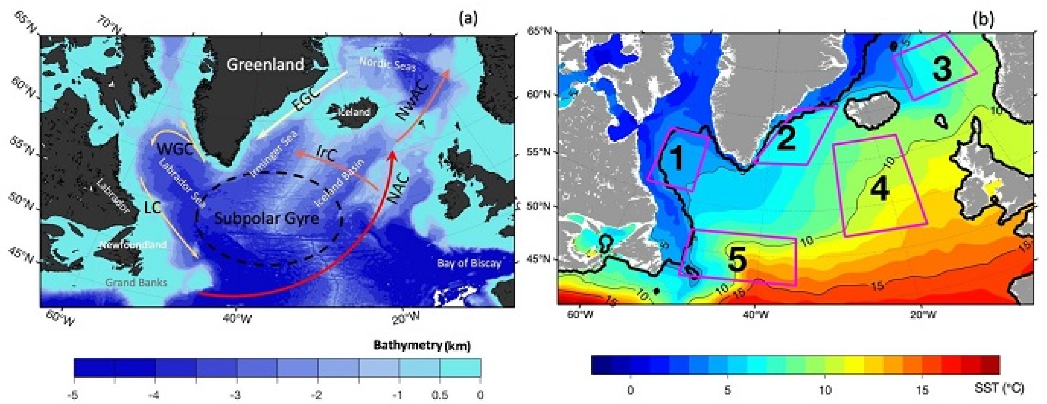
Ocean salinity in the subpolar North Atlantic (SPNA, 45–70°N, 65°W–10°E) exhibits large variability on time scales from seasons to decades and longer time scales [1,2,3,4,5]. This variability is a result of the mixing and exchange between water masses of contrasting properties: The warm, high-salinity waters that are transported by the North Atlantic Current (NAC) from the tropical and subtropical latitudes and the cold, low-salinity waters that are transported from the Arctic latitudes by the East Greenland Current (EGC) and Labrador Current (LC) [6] (Figure 1a). Characteristics of the regional salinity are also shaped by freshwater influx sourced from excessive precipitation over evaporation [7,8], seasonal ice melting and freezing, and water discharge from adjoining rivers and the Greenland ice sheet [9,10]. Salinity has a dominant effect on the stratification of the upper ocean in the SPNA and is regarded as a main driver of deep subpolar oceanic convection in the Labrador and Irminger seas [11,12], affecting the ventilation of heat, salt, anthropogenic carbon, and oxygen in the deep waters of the world ocean. Monitoring and understanding ocean salinity variability in the SPNA has long been articulated as a central element for improving modeling and prediction of the changes in subpolar water mass transformation and the Meridional Overturning Circulation (MOC) [13,14].
Traditional means of salinity monitoring rely on the measurements provided by vessels, buoys, and, more recently, Argo profiling floats. In the SPNA, these in situ measurements are sparse and rarely of sufficient resolution to resolve the spatiotemporal distribution of salinity associated with regional ocean currents (Figure 1a). Satellite remote sensing of sea surface salinity (SSS) offers a novel capability of mapping global SSS and will be of great value for complementing in situ monitoring platforms. Since 2010, satellite SSS observations are available from three missions [15]. They are the Soil Moisture and Ocean Salinity (SMOS) mission by the European Space Agency (ESA) that has been providing continuous SSS data records since its launch in November 2009 [16,17], the Aquarius/Satélite de Aplicaciones Científicas (SAC)−D mission by the National Aeronautics and Space Administration (NASA) that lasted from June 2011 to June 2015 [18,19], and the NASA Soil Moisture Active Passive (SMAP) mission that has been operating since January 2015 [20]. All three missions make use of L-band (1.4GHz) microwave radiometry operating at ~1.4 GHz (wavelength = 21 cm). Near-real-time global SSS maps are provided at spatial scale of roughly 40–50 km for SMOS and SMAP and 100–150 km for Aquarius, and with a revisit every 2–3 days for SMOS and SMAP and every 7 days for Aquarius.
Retrieving SSS from L-band radiometers arises from the fact that the observed brightness temperatures (Tb) are related to the dielectric constant of seawater, which is a function of salinity and temperature [21]. However, satellite Tb retrievals are also affected by the sea surface state (roughness, foam, and whitecaps) and external perturbing factors including extraterrestrial contributions (e.g., galactic/cosmic background radiation and sun glint), antenna-radiation emissions, Faraday rotation in Earth’s ionosphere, atmospheric attenuation, and radio frequency interference (RFI) that results from the unauthorized use of the protected L-band in some coastal areas [22,23,24,25,26,27,28]. Achieving the goal of satellite SSS measurements of 0.1–0.2 practical salinity scale (pss) accuracy [17,18] requires that all internal and external factors be fully accounted for. However, even after removal of all unwanted signals, the absolute sensitivity of Tb to SSS is still low and highly dependent on sea surface temperature (SST). The sensitivity decreases from 0.7 K per pss change for SST of 30 °C to 0.25 K per pss change for SST of 0 °C. The SST-related drop in the sensitivity puts strong demands on the retrieval of SSS from Tb measurements in the cold waters of the polar and subpolar regions.
The SPNA has complex bathymetry and hydrography, featuring cold waters in the marginal basins of the Labrador and Irminger seas (Figure 1a,b). Two-thirds of the surface area in these marginal seas are covered by ice between December and June, with SST varying between –1 °C in winter and 5–6 °C in summer. The waters are not only cold but also fresh, transported from Arctic latitudes by the East Greenland Current (EGC), the West Greenland Current (WGC), and the Labrador Current (LC) along the continental shelves [29,30]. Retrieving SSS values associated with these boundary currents is challenged by both the cold-water temperatures and the proximity to land and sea ice. At the L-band frequency, land and sea ice are radiometrically warmer than the ocean. The emissivity from land/ice surface are leaked into the radiometer receiver through side lobes or partially through the main lobe, which affect the measurement footprint [17]. The biased Tb can lead to a significant bias in SSS retrievals once the fraction of land or sea ice within the footprint exceeds 1%. Corrections for the spurious effects of land/ice contaminations are needed and have been made in all satellite SSS products [31,32,33].
There have been several studies using in situ measurements to evaluate the accuracy of satellite SSS retrievals in the challenging regions, including the marginal seas [34], coastal waters [35,36], and subarctic and Arctic oceans [37,38,39,40,41]. Tang et al. [32] used a collocation window of 12.5 km radius and 24 h and composed nearly 20,000 pairs of SMAP and in situ data for the regions north of 50°N. The SMAP data were produced by the Jet Propulsion Laboratory (JPL) for the period of 2015–2018 [33]. They showed that, although SMAP and in situ data are significantly correlated at 0.82, the root mean square difference (RMSD) is about 1 pss, which is much larger than the accuracy of 0.2 pss found between 40°S and 40°N [37,38]. They found that the RMSD estimate, though large, is consistent with the estimate obtained by other studies [37,38,39] using SMOS and Aquarius products for the Aquarius mission duration (2011–2015).
One interesting argument made by Tang et al. [32] is that the relatively large RMSD should not be regarded as the limitation of SSS measurements in the Arctic. Arctic SSS has large spatiotemporal changes with magnitudes often exceeding 3 pss. The SSS retrievals of ~1 pss accuracy would be sufficient for detecting the large SSS changes induced by seasonal freshwater influx into the Arctic region. Fournier et al. [41] offered a comprehensive, in situ-based evaluation of six available SSS products in the Arctic Ocean derived from all three SSS missions. They showed that the six products have excellent consistency among one another in describing seasonal and interannual variations associated with the sea ice cycle. Their findings support the assessment of Tang et al. [32] that the L-band radiometers should have sufficient capability to detect the cold-water SSS variability at high latitudes.
The SPNA is a region where the cold and fresh waters from the Arctic meet and exchange with the warm and salty waters from the tropical and subtropical latitudes. Several validation studies have been conducted to quantify the uncertainties in satellite-derived SSS products using ship-based measurements and/or models at high northern latitudes [37,38,39,40,41,42]. For instance, Kohler et al. [37] evaluated SSS retrievals from Aquarius and SMOS for a one-year period from May 2012 to April 2013 and showed that SMOS SSS fields had a temperature-dependent negative SSS bias of up to −2 pss for temperatures less than 5 °C. Nevertheless, the question regarding how faithful satellite SSS retrievals are in representing the basin-scale SSS variability on seasonal, interannual, and longer time scales has not been fully addressed. This study aimed to address this question and to focus attention on the applicability of satellite products to studies of SSS variations from seasonal to decadal time scales. Therefore, four SSS products from SMAP and SMOS were evaluated with reference to two in situ, gridded products.
The paper is organized as follows. Section 2 provides a description of satellite and in situ SSS datasets. Section 3 presents the analysis of seasonal, interannual, and decadal variations of SSS using harmonic analysis and statistical methods. Discussion and conclusions are given in Section 4 and Section 5.
2. Materials and Methods
Four satellite SSS products from SMAP and SMOS and two in situ-based SSS products were used in this study. Links to data download web pages are provided in the acknowledgements. The following is a brief description of each dataset.
2.1. Satellite SSS Products
2.1.1. SMOS Satellite and Products
The SMOS satellite measures microwave radiation emitted from the Earth’s surface at L-band using an interferometric radiometer, called microwave imaging radiometer using aperture synthesis (MIRAS) [16,17]. The satellite follows a sun-synchronous polar orbit at 763 km altitude with a 6 a.m. LST (Local Solar Time) ascending equator crossing time and a 6 p.m. LST descending equator crossing time. SMOS achieves a complete global coverage every three days with multi-incidence-angle observations at full polarization across a 900 km swath. The range of incidence angles varies from 0 to about 40 degrees over the field-of-view and the resolution changes with the angle of incidence. This setting produces an average radiometer resolution of about 40 km. The mission-required accuracy is 0.1 pss when measurements are averaged monthly on 200-km scale.
Two SMOS SSS products were used here. One was the SMOS SSS Level 3 maps produced by Laboratoire d’Océanographie et du Climat (LOEACN) and the Ocean Salinity Expertise Center (CEC-OS) of Centre Aval de Traitement des Donnees SMOS (CATDS) [43,44]. This product is referred to as SMOS LOCEAN in the following discussion. The current fourth version has corrected systematic biases using an improved de-biasing technique, which improves ice filtering and SSS at high latitudes [44]. The nine-day running mean maps are available from January 2010 onward.
The other SMOS product was the Level 3 version 2 SMOS SSS global product from the Barcelona Expert Center (BEC) [45]. The products are generated from a de-biased non-Bayesian approach [46] that corrects the systematic biases caused by the presence of land masses and radio interference, and improves the data gaps due to the non-convergence of the retrieval algorithm. The nine-day running objectively analyzed Level 3 (L3) maps were provided daily at 0.25° × 0.25° spatial resolution and available from January 2011 to December 2019. This product is referred to as SMOS BEC in this study.
2.1.2. SMAP Satellite and Products
The SMAP satellite is a conically scanning, wide-swath, single-channel, L-band radiometer, scanning the Earth’s surface at a constant incidence angle of 40° through the rotation of the reflector around the nadir axis [20]. The satellite is in a near-polar, sun-synchronous orbit at an altitude of 685 km. An ascending node crossing occurs at 6 p.m. and a descending node crossing at 6 a.m. local time. With a ~1000-km-wide swath and an eight-day repeat cycle, the instrument achieves a global coverage in approximately three days with a spatial feature resolution of about 40 km.
The study used two SMAP SSS maps produced by two groups. One was the SMAP Level 3 version 4.3 JPL product (hereafter referred to as SMAP JPL), featuring a 60-km spatial resolution and distributing eight-day running mean dataset based on the repeat orbit of the SMAP mission and also a monthly average dataset, both on 0.25° × 0.25° grids [47]. The JPL SMAP SSS algorithm [33] includes an improved land/ice correction and is able to retrieve SSS in ice-free regions within 35 km of the coast [32].
The other product was the SMAP Level 3 Remote Sensing Systems (RSS) product (hereafter referred to as SMAP RSS) recently released version 4.0 [48]. The product is resampled onto 0.25° × 0.25° from a 70 km spatial resolution using a Backus–Gilbert-type optimum interpolation (OI) in order to reduce random noise [31] and mapped monthly and eight-day running mean. Noted improvements in the version 4.0 product include an improved land correction that allows for salinity retrievals within 30–40 km of the coast, use of sea-ice mask derived from RSS AMSR-2, and implementation of a sea-ice threshold of 0.3% (gain weighted sea-ice fraction).
Both SMAP products are available from April 2015 to the present and distributed by the NASA Physical Oceanography Distributed Active Archive Center (PO.DAAC).
2.2. In Situ Gridded SSS Products
Two in situ gridded SSS products were included as a base reference for satellite-derived SSS products. One was the Roemmich–Gilson Argo monthly Climatology [49] (hereafter referred to as Argo) and the other is version 4.2.1 of the Met Office Hadley Centre “EN” series monthly objective analyses [50] (hereafter referred to as EN4). The Argo RG dataset is constructed from more than 3000 autonomous profiling floats over the global ocean. It is obtained by first estimating the mean field using a weighted local regression fit to several years of Argo data and then performing optimal interpolation on the mean-subtracted monthly residuals to obtain the interpolated anomaly fields on 1° × 1° grids. The salinity data of the topmost layer at the depth of 2.5 m were used as SSS in the analysis.
The EN4 1° × 1° gridded monthly data products are compiled from quality controlled temperature and salinity profiles that are sourced from the Global Temperature and Salinity Profile Programme (GTSPP), World Ocean Database 2009 (WOD09), and Argo. The use of non-Argo data is essential in regions where Argo floats are limited or not available, and shallow coastal waters, marginal seas, and sea-ice marginal zones. The EN4 dataset provides more spatial coverage than the Argo dataset in areas like the Labrador and Irminger seas. The topmost grid level of EN4 is at the depth of 5.25 m below the surface, and is used for comparison with satellite SSS products.
One caveat of the in situ-based evaluation is the uncertainty associated with the differences in measurement depth. Satellite SSS retrievals represent the salinity in the ocean surface skin layer that is penetrated by electromagnetic radiation. The L-band microwave penetration depth, defined as the depth at which the incoming power density is reduced exponentially by two orders of magnitude, is about 1 cm [51]. The topmost salinity in Argo and EN4 products is obtained by optimal interpolation at the depth of 5 m and commonly referred to as bulk SSS. The skin and bulk SSS can be different if vertical salinity gradients exist between the two measurement depths [28,52]. It is yet to be known how significant the vertical salinity gradient within the topmost 5 m in the SPNA and how large the skin-bulk SSS differences are. Therefore, degree of caution should be exercised when interpolating the findings of the study.
2.3. Methods
The two in situ products, Argo and EN4, are available on a monthly basis. To be consistent, monthly mean fields were constructed for all four satellite products and used in the study. In addition, the Argo product is available only for the open ocean and the EN4 product has large uncertainty in the marginal ice zone. Both in situ products are not suitable as a reference within the marginal ice zone (Figure 1b). Hence, the main focus of this study was on the SSS variability over the ice-free open area in the SPNA, spanning 65°W to 10°E in longitude and 45°N to 70°N in latitude.
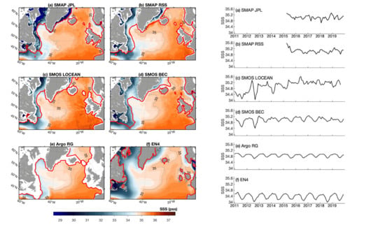
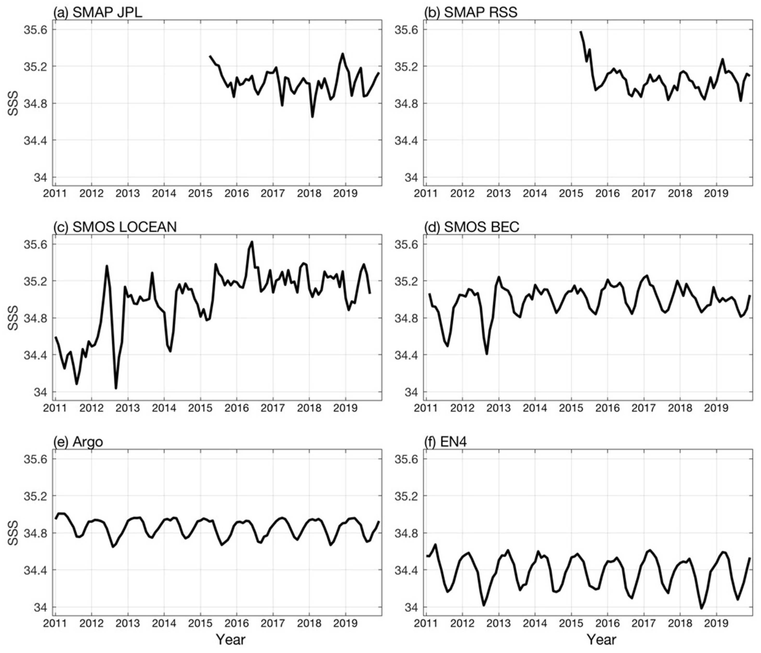
The monthly mean time series constructed from averaging over the permanent ice-free grids are shown for the available duration of each data product between 2011–2019 (Figure 2). The mean values of satellite products are generally higher than Argo and EN4. The satellite time series fluctuate above 34.8 pss, while the in situ products are either at this mean level (Argo) or below it (EN4). On seasonal timescales, Argo and EN4 time series are dictated by a periodic pattern, with higher SSS in spring and lower SSS in summer. The seasonal periodicity is seen in SMAP RSS and SMOS BEC, but not readily identifiable in SMAP JPL and SMOS LOCEAN. For the entire time period (2011–2019), the time series of Argo and EN4 showed no obvious trend. SMOS LOCEAN had a peculiar upward trend and large interannual variations before 2016. There were also abrupt changes in SMOS BEC in the first 2–3 years of its data record. The large differences between satellite and in situ products in terms of mean value, seasonality, interannual, and longer-term changes called for a systematic approach to evaluate the cause of the differences in the products.
In this study, seasonal variations of SSS in the products were examined using harmonic analysis. The analysis was applied to the three full years from 2016 to 2018, during which SMOS and SMAP overlapped one another and SMOS time series had no large trends (or drifts). At each grid point, a least squared fitting of the annual and semiannual harmonics to the time series was performed based on the following equation [53]:
where S is the monthly mean SSS at time t expressed in months, S0 is the mean annual salinity, ω1 and ω2 are the annual and semiannual frequencies expressed as ω1 = 2π/12 months and ω2 = 2π/6 months, and a1, a2, φ1, and φ2 are the estimated regression coefficients for the amplitudes and phases of the annual and semiannual harmonics, respectively. Applications of a least-squared fitting to the seasonal cycle of salinity have been made in several previous studies [54,55].
Interannual SSS variations were obtained by subtracting the annual and semiannual signals from the time series. Spatial patterns of the corresponding SSS anomaly maps at interannual timescale were examined for the SMOS decade (2011–2019).
3. Results
3.1. Mean SSS Pattern
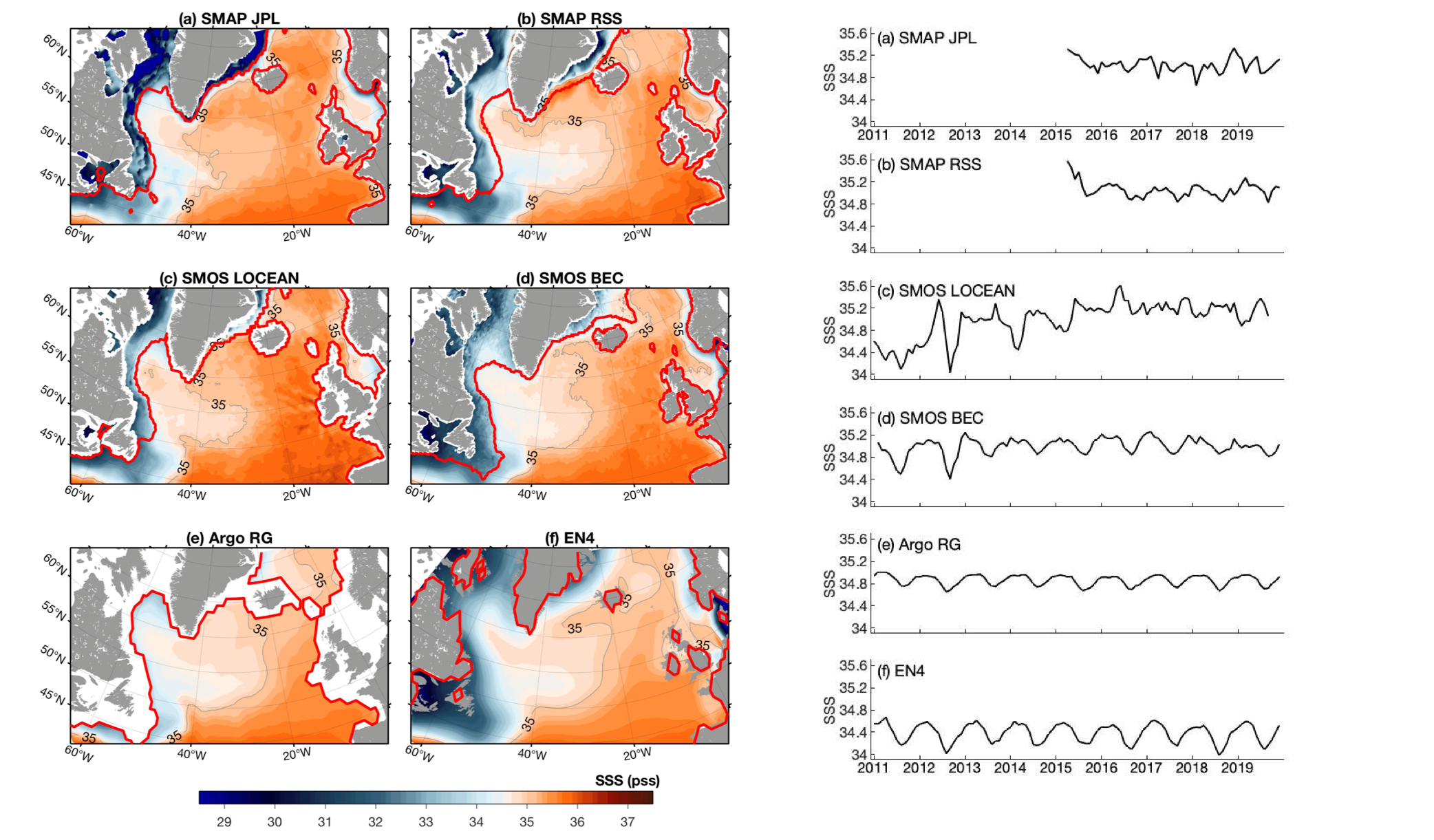
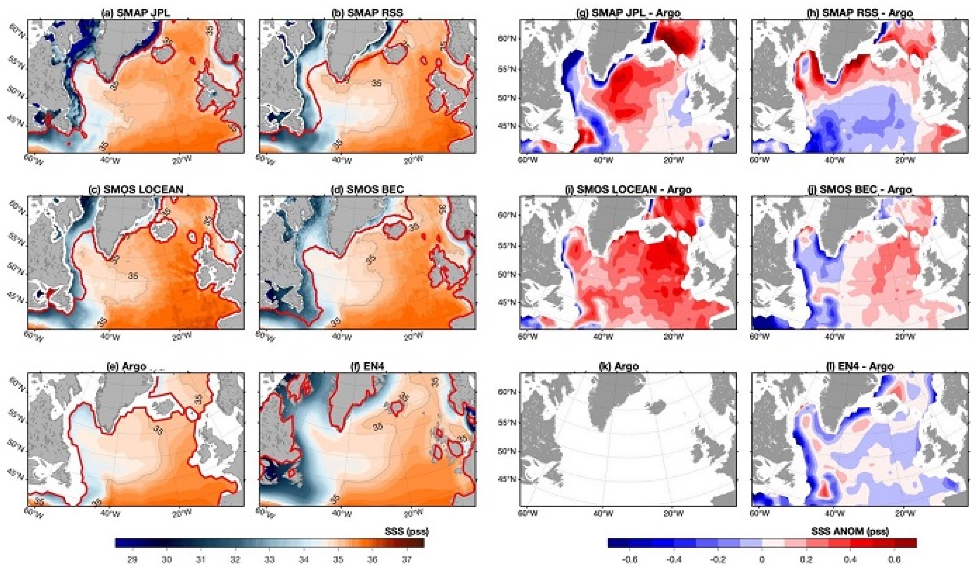
The six mean SSS patterns averaged for the period 2016–2018 are shown in Figure 3a–f. These patterns were constructed from SSS values at all available grids, including those within sea-ice marginal zone. The boundary between the permanent ice-free ocean and the seasonal ice zone was also extracted from each dataset and superimposed in Figure 3 (denoted by solid red lines). In the seasonal ice zone, SSS values were available only in summer ice-melting months. SMAP JPL showed large spatial variability of SSS in the seasonal ice zone, which may be related to the inclusion of an improved land/ice correction that allows SSS to be retrieved within 35 km of the coast in ice-free conditions [32]. For the Argo SSS field, the ice margin was the boundary of available data points, because Argo floats have observations only in ice-free open ocean. The EN4 SSS field had no ice margin, as the objective analysis referred to a long-term climatology in regions of no observations [50] and, hence, those values over the continental shelves, where the surface is mostly covered by sea ice during winter, may have large uncertainties.
The six mean fields agreed broadly on the spatial distribution of the time-mean SSS in the SPNA. Surface waters are saltier in the eastern SPNA, owing to the northward transport of warm and salty surface waters from the tropical/subtropical latitudes by the NAC. Surface waters are fresher in the western marginal seas like the Labrador and Irminger seas, with the lowest SSS values following the pathways of the EGC and WGC off Greenland and LC off Labrador and Newfoundland. The contrast between the fresh and salty surface waters is largest in the open ocean to the east of the Great Banks of Newfoundland near 40°W, 45°N, where the cold and fresh LC meets the warm and salty Gulf Stream.
Despite the similarity in spatial pattern, the six mean SSS fields differed considerably in magnitude. To see this more clearly, SSS mean difference fields in reference to Argo SSS are shown (Figure 3g–l). Positive anomalies denote the product SSS values were higher than Argo SSS (i.e., the sea surface is saltier than Argo) and vice versa for negative anomalies. SMAP JPL was lower (fresher) near continental shelves of Greenland, Labrador, and Newfoundland and higher (saltier) than Argo SSS in the open sea. SMAP RSS showed that the anomalies changed the sign at around 52°N, featuring negative (fresh) anomalies south of the latitude and positive (salty) anomalies north of the latitude. Positive anomaly differences were greater than 0.4 pss in the Labrador and Irminger seas. SMOS LOCEAN was saltier than Argo SSS over the entire basin. SMOS BEC was saltier east of 40°W and fresher west of the longitude. The differences between EN4 and Argo tended to be large (~0.3 pss) near the ice margin in the Irminger and Labrador seas, and the differences were generally small, less than 0.1 pss, in the open sea.
3.2. SSS Variances
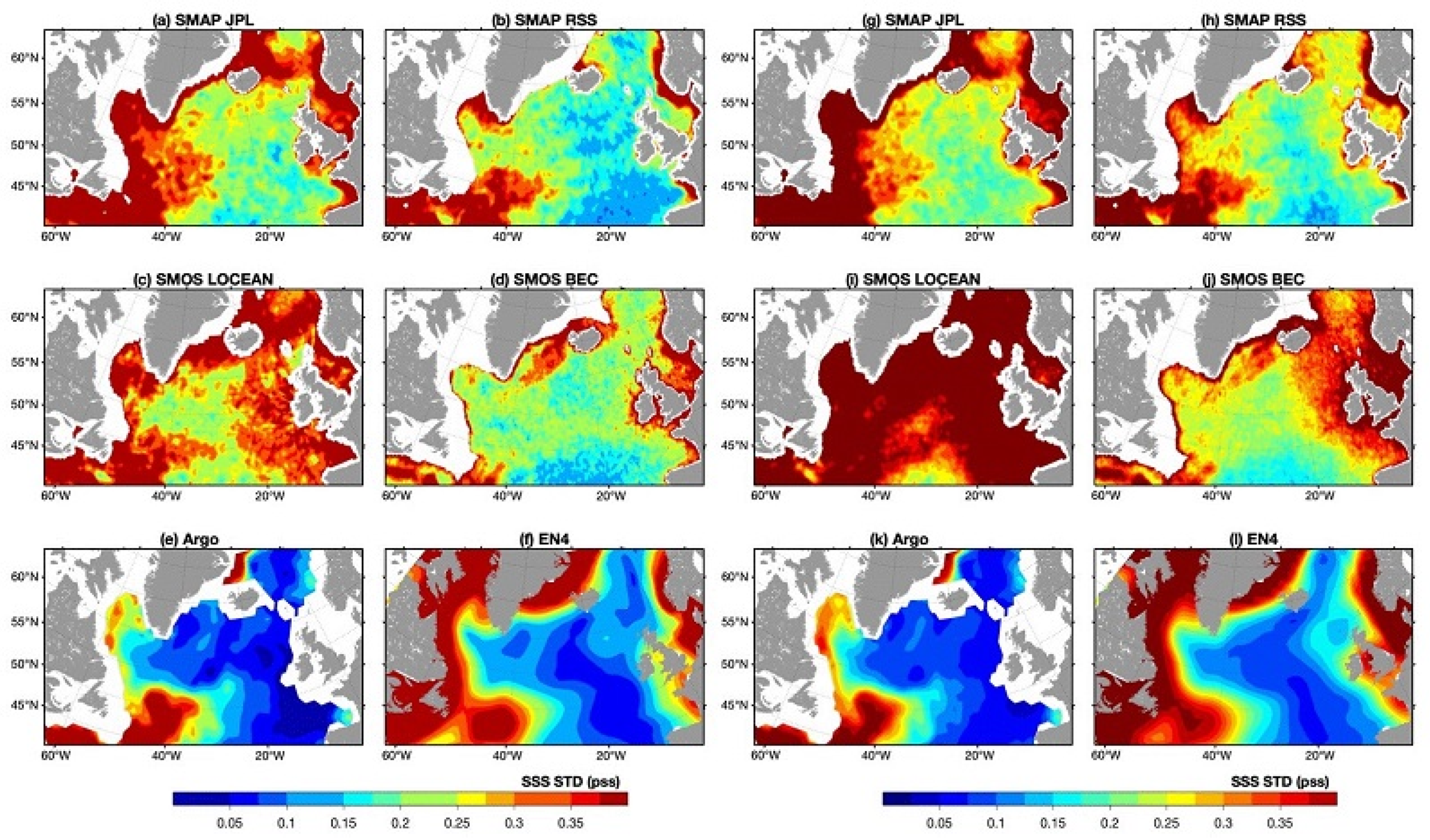
To evaluate the spatial pattern of variability, standard deviations (SD) of monthly mean SSS fields were computed for two periods: The three-year overlap period (2016–2018) for all six products (Figure 4a–f) and the maximum available period for each product during 2011–2019 (Figure 4g–l). In the latter computation, the period for SMAP JPL and RSS products spanned from May 2015 to December 2019, and the period for SMOS products was from January 2011 (February for SMOS BEC) to December 2019. Argo and EN4 were available for all months between 2011 and 2019.
For the three-year overlap period, satellite SSS variability was generally small (SD < 0.2 pss) in the open sea and large (SD > 0.4 pss) over the eastern and western continental shelves and in the marginal seas, particularly the Labrador Sea (Figure 3a–f). Overall, the SD values in SMAP JPL and SMOS LOCEAN were noticeably higher than those in SMAP RSS and SMOS BEC, and the SD in all satellite products was higher than those in the two in situ products. Both in situ products indicated that the SD was small, less than 0.1 pss for the salty surface waters in the open sea, where the SDs in all satellite products were at 0.1 pss and greater. The difference between satellite and in situ products over the open sea indicated that satellite products have a higher noise level.
For the extended period that included all months available between 2011–2019, the SD patterns produced by satellite products showed a various degree of enhancement (Figure 3g–j). The SD in SMAP JPL and RSS enhanced in the marginal seas, while those produced by SMOS products enhanced substantially over the entire SPNA. The SD in SMOS LOCEAN was greater than 1 pss over almost all areas and the SD in SMOS BEC exceeded 0.3 pss in the eastern basin. This change of the SD pattern with time period indicated that the two SMOS products had basin-scale time varying biases. On the whole, the four satellite products provided four different SD patterns, and all deviated substantially from the in situ-based SD patterns.
3.3. Annual Cycle
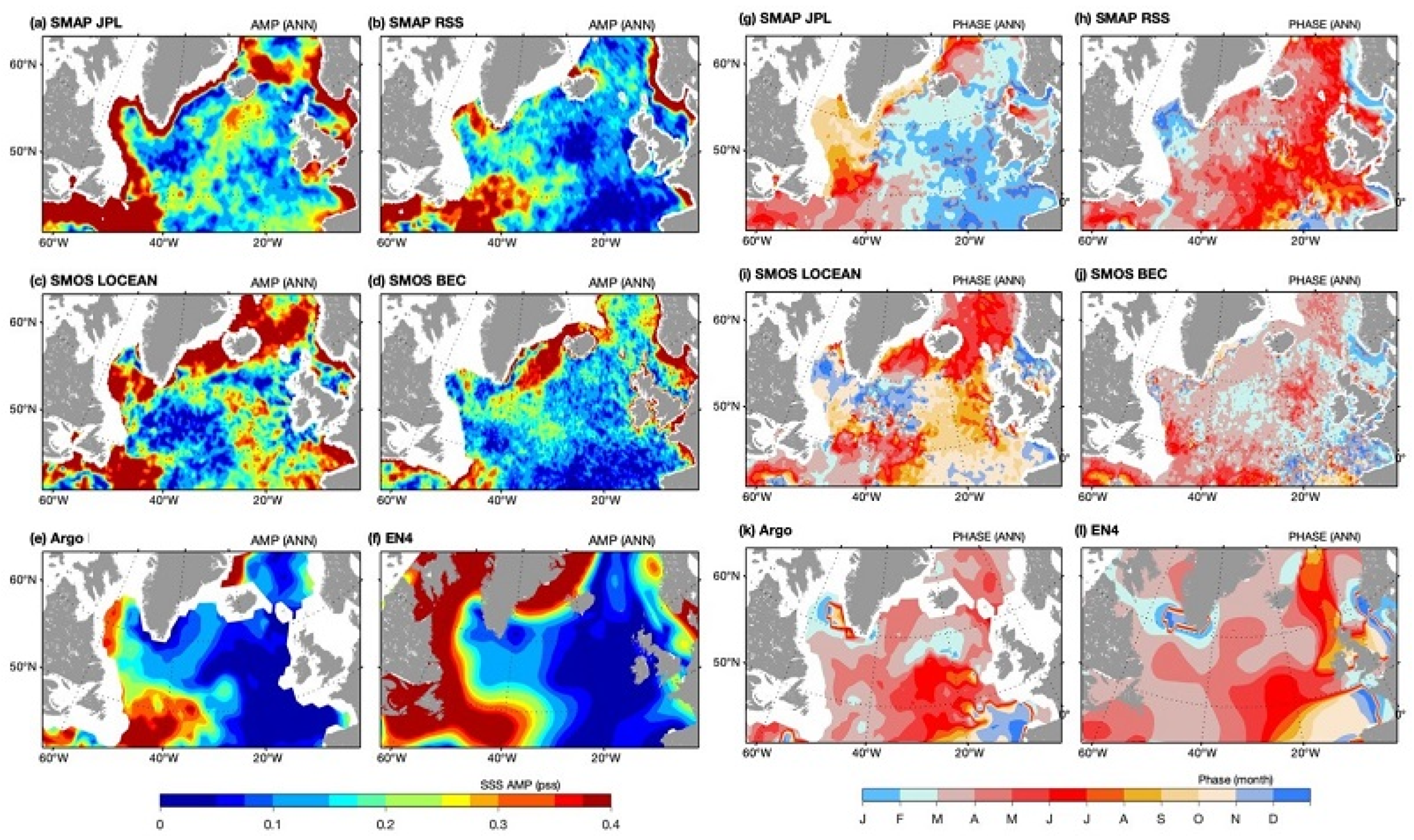
The amplitudes (a1 in Equation (1)) of the annual cycles estimated from harmonic analysis (Figure 5a–f) showed that the products agreed broadly on the basin-scale pattern. Smaller annual amplitudes (<0.2 pss) were located in the open basin where the mean SSS values were higher, while larger annual amplitudes (>0.3 pss) occurred over the eastern and western continental shelves and the Labrador Sea where the mean SSS values were lower. Larger amplitudes were also seen in the open sea to the east of the Grand Banks of Newfoundland near 45°N, 40°W where SSS gradients are large. Compared to the mean patterns (Figure 3), the areas that are dominated by salty surface waters had a weak annual cycle and, conversely, the boundary regions that are influenced by low-salinity water influx from high latitudes had a strong annual cycle. The amplitude distribution is similar to the pattern of the SD (Figure 4), implying the dominance of the annual variations in the total variances of SSS.
Despite the overall agreement on the basin-scale pattern, the amplitude distribution of the four satellite products differed from each other and from the two in situ products in spatial details. In general, SMAP RSS resembled that of Argo and EN4 away from the coasts. By comparison, SMAP JPL had large amplitudes encircling the sea ice margin in the western marginal seas (>0.4 pss). It also had noticeably large amplitude in the Reykjanes Ridge area south of Iceland (~0.3 pss). SMOS LOCEAN had a band of exceptionally large amplitudes in the Irminger and Nordic Seas and the Bay of Biscay near 45°N, 10°W. SMOS BEC deviated from the two in situ products in two areas: The Irminger Sea, where the amplitudes of SMOS BEC were unusually larger, and the open ocean east of the Grand Banks of Newfoundland near 45°N, 40°W, where the amplitudes were significantly weaker.
The phases (φ1) of the estimated annual cycles (Figure 5g–l) represent the time (month of the year) at which the maximum amplitude of the SSS annual cycle occurred. The phases varied from 0 to 360°, with each month representing 360/12 degrees (or 2π/12 radians) of the total cycle. The phase distribution in Argo and EN4 showed a southeastward–eastward increase, suggesting that the maximum amplitude of the annual cycle (i.e, the saltiest surface water) progressed from January-Febraury in the Labrador Sea, to May-June in the western SPNA, and to October–November toward the Bay of Biscay near 45°N, 10°W. Of the four satellite SSS products, the phases in SMAP RSS were similar to those of Argo and EN4, while the phases in SMAP JPL were completely opposite to Argo and EN4. The phases in the two SMOS products differed considerably from each other and from the two in situ products.
3.4. Semiannual Cycle
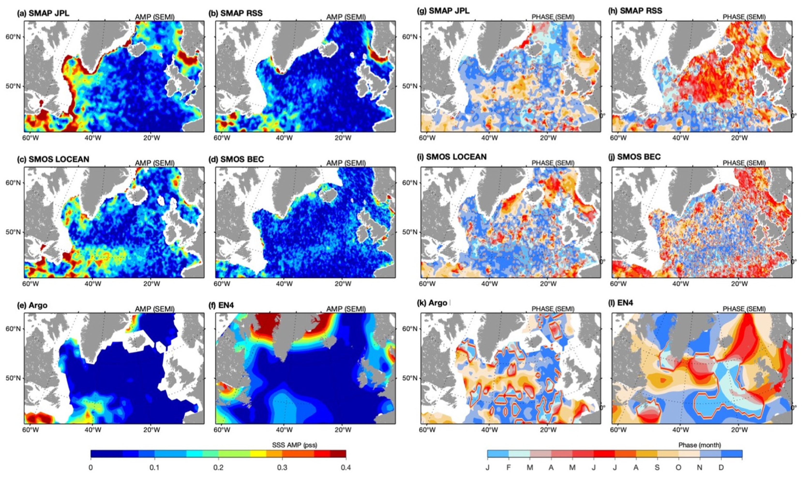
The amplitudes (a2) of the estimated semiannual cycles (Figure 6a–f) were generally small in Argo and EN4. Amplitudes of ~0.2 pss were visible in two areas, east of the Grand Banks of Newfoundland around 45°N, 40°W and the East Greenland shelf north of 60°N. The satellite products also had a weak semiannual component except for SMAP JPL. In the latter, larger amplitudes (>0.4 pss) of the semiannual cycle encircled the sea-ice margins in the Labrador and Irminger seas, and the North Sea around 55°N, 0°. SMAP RSS had also unusually large amplitudes (>0.4 pss) in the North Sea.
The phases (φ2) of the estimated semiannual cycles (Figure 6g–l) varied with products. Argo and EN4 agreed with each other in the western basin but deviated from each other in the eastern basin and the Nordic Seas. The phases in SMAP JPL appeared to have good consistency with those of Argo, but the phases in other three satellite products were off by a signifiant degree.
3.5. Seasonal Variations of SSS in Five Selected Areas
Five areas were selected to evaluate the seasonal variations of SSS that are represented by the annual and semiannual cycles. These five areas are depicted in Figure 1b and included the central Labrador Sea (referred to as Box 1 LS), the Irminger Sea (Box 2 IrS), the Nordic Seas (Box 3 NS), the region influenced by the NAC (Box 4 NAC), and the open ocean east of the Grand Banks of Newfoundland (Box 5 GB). Boxes 1 and 2 were in areas featuring fresher surface waters, while Boxes 3 and 4 were in areas featuring saltier surface waters. Box 5 was in an area of large SSS gradients.
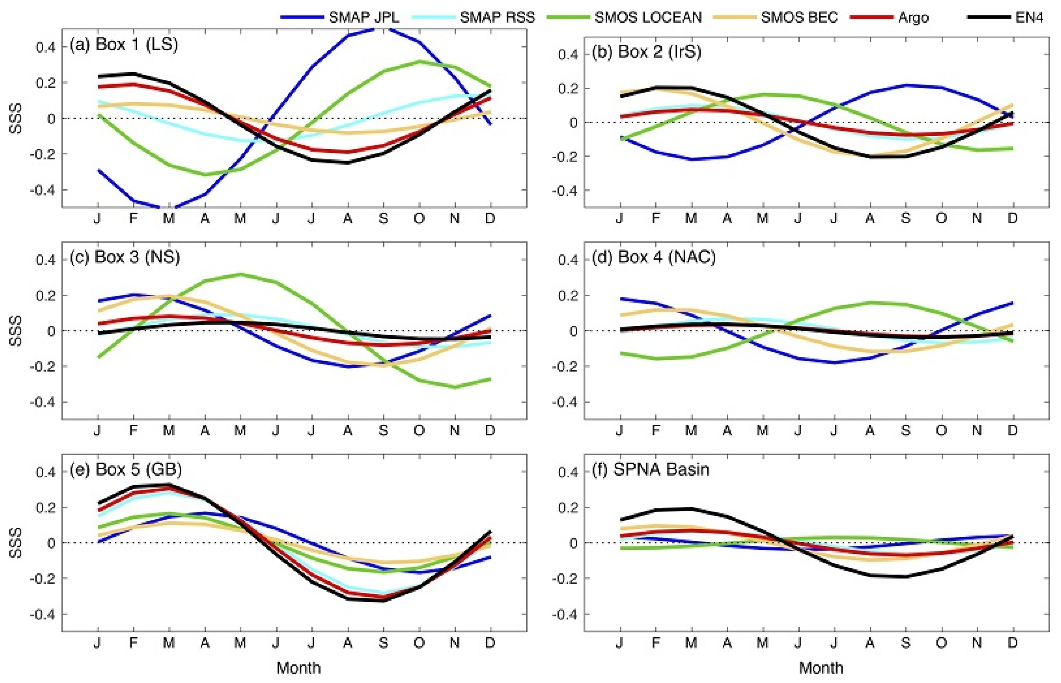
Time series of the annual cycles averaged over the five boxes together with the basin average are shown in Figure 7. Argo and EN4 had similar annual cycles at all locations except for Box 2 (IrS) and the basin average, where the annual amplitude of EN4 was greater than that of Argo. The reason is that EN4 had more SSS values over the continental shelves in the marginal seas where surface waters are fresher and have stronger annual amplitudes.
The annual phases of SMAP JPL were completely opposite to those of Argo and EN4 in Boxes 1 and 2. The phases were also shifted by several months in Boxes 3–5. This finding was consistent with Figure 5, in which the annual cycle of SMAP JPL was out of phase with in situ products over almost the entire basin. SMOS LOCEAN also did not do well, as there were obvious phase shifts in Boxes 1–4. SMAP RSS was out of phase in Box 1, while having a good coherence with in situ products in all other boxes. SMOS BEC had a weak amplitude in all boxes and a slight phase shift in Boxes 3–4. Overall, a broad agreement between all six products was achieved only in Box 5.
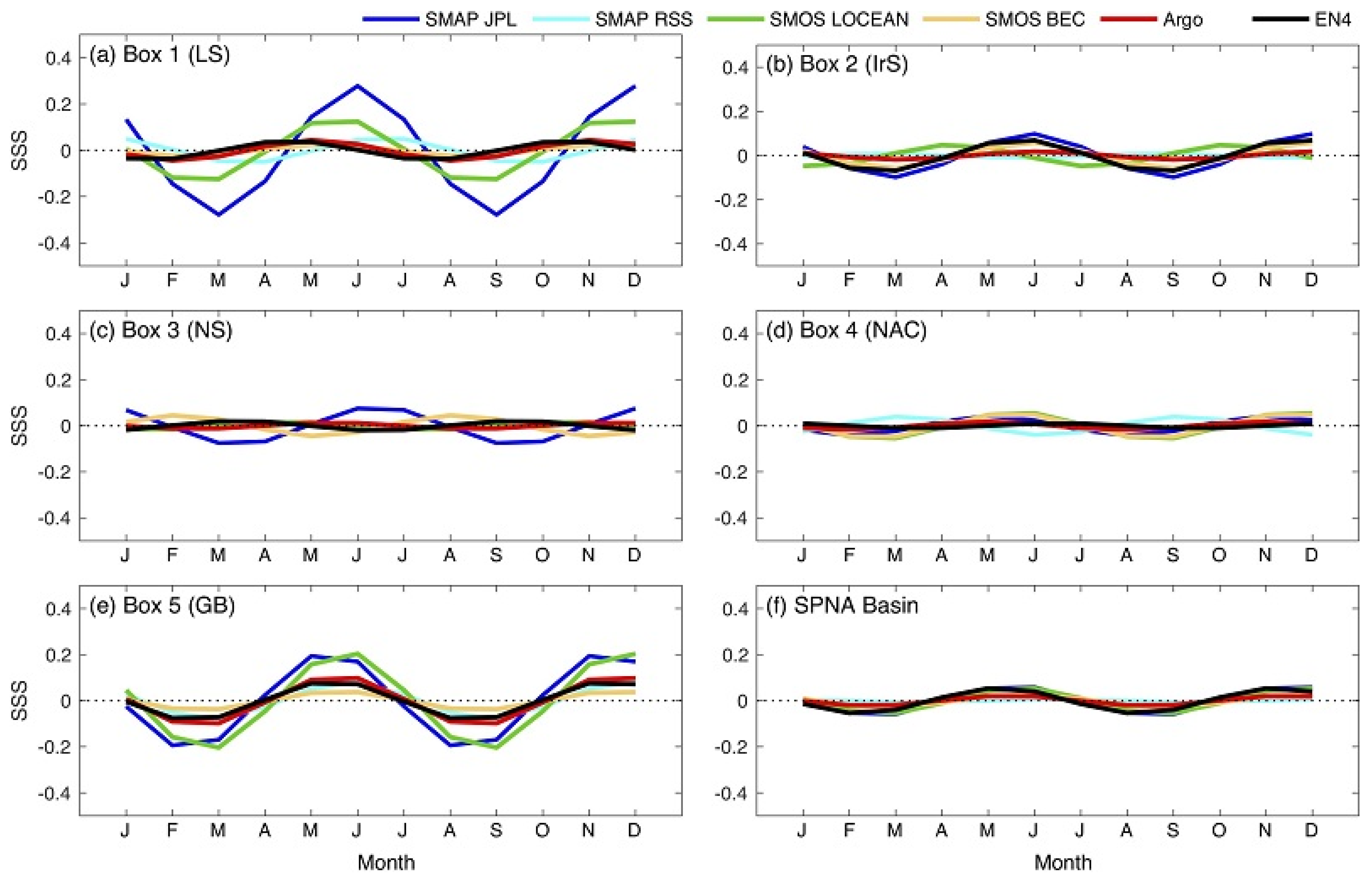
Time series of the semiannual cycles in the five boxes and over the basin (Figure 8) showed that the semiannual variations in Argo and EN4 were weak (<0.05 pss) in all areas except for Box 5, where SSS increased in spring and fall and decreased in summer. SMAP JPL and SMOS LOEAN had the semiannual maxima and minima well produced in Box 5, but had wrong phases in Box 1. SMAP RSS and SMOD BEC were weak and mostly out of phase with Argo and EN4.
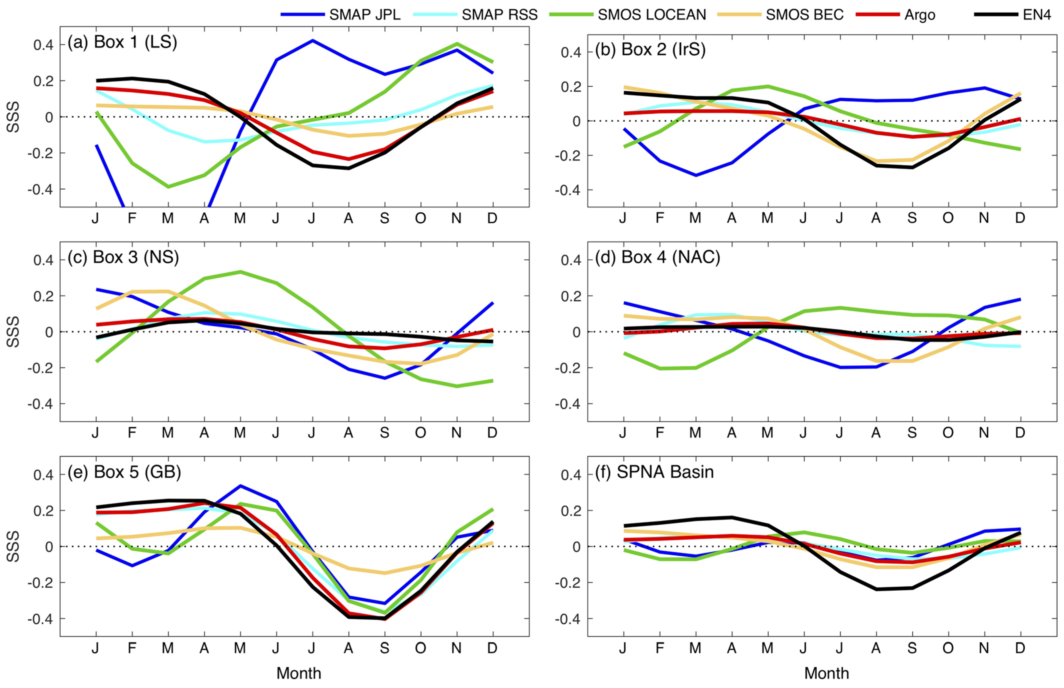
Seasonal variations of SSS at any given grid in the SPNA could be reconstructed by combining the annual and semiannual cycles estimated from harmonic analysis. This allowed the seasonal variations at different SSS regimes to be interpreted in terms of the annual and semiannual contributions. The reconstructed seasonal cycles for the five boxed areas and the SPNA basin are shown in Figure 9. Argo and EN4 indicated that the seasonality at all locations was dominated by the annual cycle. In the fresher water regime (Boxes 1–2), in situ-based SSS were higher in winter and lower in summer with an amplitude of about 0.2 pss. In the saltier water regime (Boxes 3–4), seasonal variability in in situ products was weak, increasing slightly (<0.05 pss) in spring and decreasing slightly in late summer. In the area of large SSS gradients (Box 5), SSS varied strongly on the annual basis, with higher SSS (~0.2 pss) in winter and spring and lower SSS (~–0.4 pss) in summer. The high SSS seasons appeared to last longer than the low SSS seasons, though the amplitudes of high SSS (~0.2 pss) were about half of the amplitudes of low SSS (~–0.4 pss).
The asymmetry of the SSS seasonal variations in Box 5 was a result of composition of different phases of the annual and semiannual cycles. The synchrony between the minima of the annual and semiannual cycles in summer enlarged the annual amplitudes of low SSS. Meanwhile, the combination of opposite phases of the annual and semiannual cycles in winter and spring weakened the annual amplitudes of high SSS but lengthened the duration. For Boxes 1–4, the semiannual component was small and did not impose any significant effect on the annual cycle.
3.6. Main Characteristics of the Annual and Semiannual Variations
Main characteristics of the estimated annual and semiannual cycles and the reconstructed seasonal variations are listed in Table 1. These characteristics include amplitude, timing of SSS maximum, timing of SSS minimum, and also the correlation coefficient of each product with respect to Argo. The values are the averages over the entire SPNA and represent a quantitative summary of Figure 7f, Figure 8f, and Figure 9f.
The four satellite products showed that the amplitudes of the annual cycle were in the range of 0.03 pss (SMOS LOCEAN) and 0.06 pss (SMAP RSS), which was comparable to Argo (0.07 pss) but considerably smaller than EN4 (0.19 pss) (Figure 7f). The larger amplitude in EN4 was caused by the large annual cycle in the Labrador and Irminger seas, where EN4 had values at all grids while other products had values only during summer seasons when ice melts. Despite the differences in amplitude, the phases of EN4 highly correlated with Argo (0.99). The phases of SMAP RSS and SMOS BEC also had good correlations with Argo at 0.96 and 0.94, respectively. The phases of SMAP JPL and SMOS LOCEAN, however, had poor correlations with those of Argo, registering a low coefficient of 0.16 for SMAP JPL and a negative coefficient of −0.62 for SMOS LOCEAN.
Argo and EN4 indicated that the amplitudes of the semiannual cycle were small, about one-quarter of their respective amplitudes of the annual cycle (Figure 8f). SMAP RSS and SMOS BEC yielded a similar result, but SMAP JPL and SMOS LOCEAN were different. The latter two had stronger semiannual amplitudes, and had phases in synchrony with those semiannual phases of Argo and EN4. This is the main reason that SMAP JPL and SMOS LOCEAN correlated highly with Argo semiannual cycles at 0.99 and 0.97, respectively. SMAP RSS had a low correlation of 0.52, because its semiannual phases over most of the basin were out of phase with those of Argo (Figure 8).
The time series reconstructed from the annual and semiannual cycles (Figure 9f) indicated that the annual variations dictated the seasonality of the four products: Argo, EN4, SMAP RSS, and SMOS BEC. SMAP RSS and SMOS BEC correlated with Argo, both at 0.93, but the time of the SSS maximum was about 1–3 months ahead of Argo. On the other hand, the seasonality of SMAP JPL and SMOS LOCEAN was dominated by the semiannual variations, with the first and second maxima occurring in December and May for SMAP JPL and in June and November for SMOS LOCEAN. The two products correlated poorly with Argo, at 0.34 (SMAP JPL) and –0.02 (SMOS LOCEAN), respectively.
The respective contributions of the annual and semiannual components to seasonal variations of SSS in the SPNA were quantified in terms of the percentage of SSS variances for each component (Table 2). It showed that the four products, Argo, EN4, SMAP RSS, and SMOS BEC, were dominated chiefly by the annual variances. Argo and EN4 suggested that the annual component explained about 91–93% of SSS variances over the period of 2016–2018, while the semiannual component contributed to about 6–7% variances. SMOS BEC had the annual variations accounting for about 87% and the semiannual variations for about 12%. SMAP RSS had the annual and semiannual components that explained about 78% and 10%, respectively, of the total SSS variances. Of these four products, the combination of the annual and semiannual components accounted for 98–99% of the total variances in Argo, EN4, and SMOS BEC, but only 88% of the total variances in SMAP RSS. The contribution of the annual variances in the latter was about 10% less than that in the other three products.
By comparison, the SSS variances in SMAP JPL and SMOS LOCEAN were explained mainly by the semiannual component in the amount of 61% and 78%, respectively. The variances that came from the annual signal accounted for 35% (SMAP JPL) and 13% (SMOS LOCEAN) of the respective total variances.
3.7. Interannual Variations
Interannual anomalies of SSS in SMOS and in situ products were obtained by removing annual and semiannual cycles from harmonic analysis of the 2016–2018 period. The three-year period was selected as the base reference because this was a period during which the time series of SMOS products showed no apparent drift (Figure 2). Since the SMAP data record was short, interannual variations in the two SMAP products were not examined here.
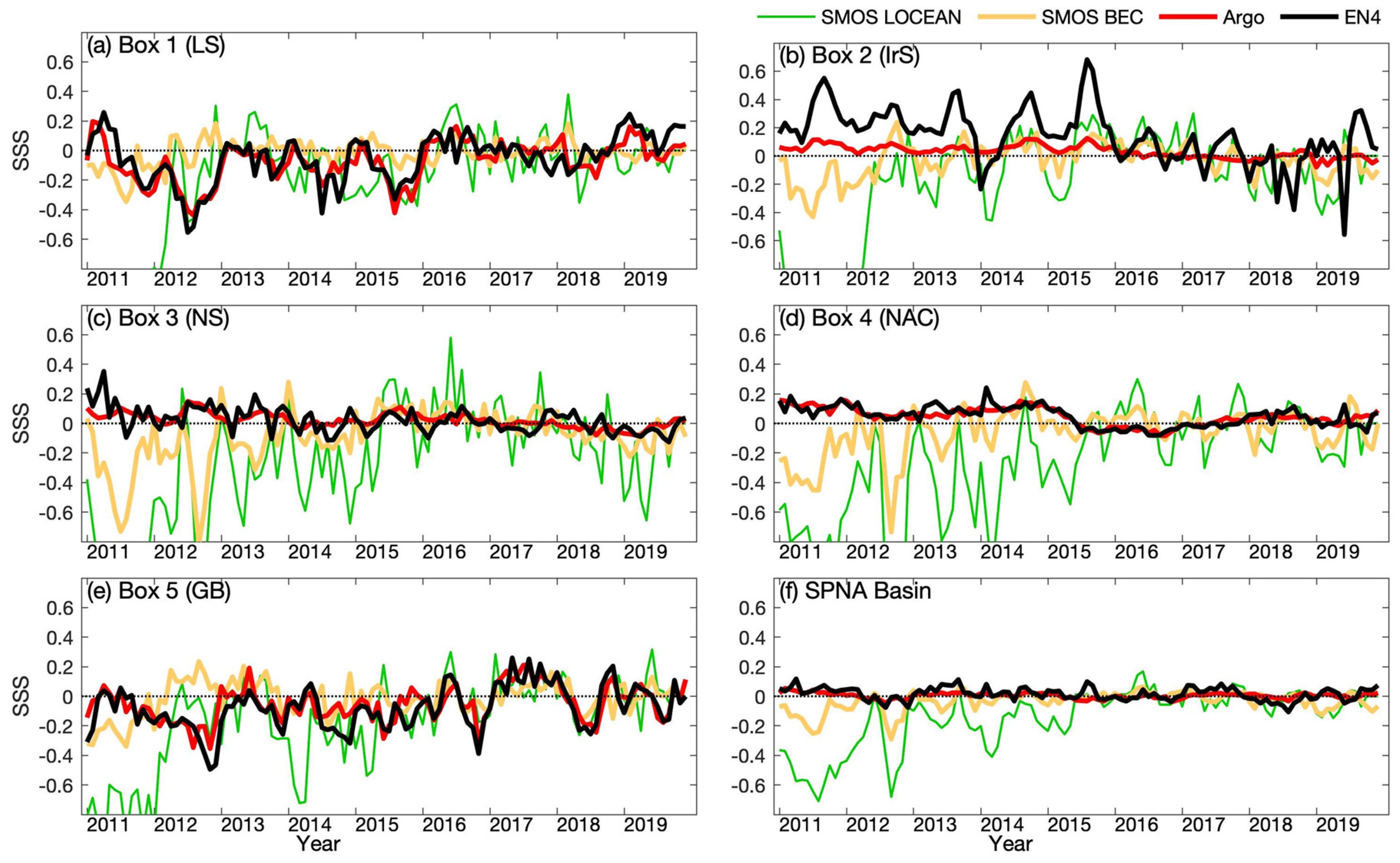
Monthly mean time series of SSS anomalies at the five selected areas and over the entire SPNA are shown in Figure 10. It is worth noting that Argo and EN4 showed no clear decadal trends during 2011–2019 when averaged over the entire SPNA, but trends were present in all five boxed areas. There were upward trends (salinification) in Box 1 (LS) and Box 5 (GB), and downward trends (freshening) in Box 2 (IrS) and Box 3 (NS). SSS in Box 4 (NAC) decreased slightly in 2015–16 and has since been recovering. The validity and implications of the trends were, however, beyond the scope of this study.
Argo and EN4 agreed well at all locations except for Box 2 (IrS), where Argo showed that interannual variations were weak, with anomaly magnitudes not exceeding 0.1 pss. Interannual fluctuations in EN4 were strong, with anomaly magnitudes varying from 0.2 to 0.6 pss. The cause of the difference may mostly be the poor data coverage in the Irminger Sea as Argo floats seldom sampled shallow seas and coastal areas.
The two SMOS products had much larger interannual anomalies at all selected areas. SMOS LOCEAN was significantly underestimated before 2013, with negative anomalies exceeding the y-axis limit of −0.8 pss in all five boxes. SMOS BEC was also drifted low, but to a lesser degree. The two SMOS time series from 2013 onward appeared to align better with Argo and EN4.
To assess the consistency between SMOS and in situ products for the period of 2013–2019, the standard deviations and correlations with Argo were computed for the selected boxes and over the entire basin (Table 3). Argo had low SD, ranging from 0.04 to 0.11 pss across the basin. Larger SD occurred in Box 1 (LS) and Box 5 (GB), where the freshwater influence was large. As expected, EN4 differed from Argo in Box 2 (IrS), where EN4 SD was 0.2 pss while Argo SD was only 0.04 pss. Argo and EN4 had a higher correlation (~0.8) in the salty-water-dominated open ocean (Boxes 4 and 5), and a lower correlation (~0.5–0.6 pss) over the freshwater-dominated continental shelves’ region (Boxes 2 and 3). Correlation was about 0.7 in Box 1 (LS). All correlation coefficients were statistically significant at a confidence interval of 95%.
The interannual SD of the SSS anomalies in SMOS LOCEAN ranged from 0.17 to 0.26 pss, which were substantially larger than Argo and EN4. The SD in SMOS BEC ranged from 0.06 to 0.12 pss, comparable to the in situ products. The most important feature missing in the two SMOS products was the regime-dependent variations in the magnitude of SD. The SD of Argo and EN4 was larger in the fresher water regimes (Boxes 1, 2, and 5) and smaller in the saltier water regime (Boxes 3–4). The two SMOS products did not have this feature.
The correlation between SMOS LOCEAN and Argo was around 0.31–0.34 in all boxed areas except for the Box 4 (NAC), where the correlation was negative. The correlation between SMOS BEC and Argo changed with area. Low correlations (0.14–0.15) occurred in Boxes 1 (LS) and 4 (NAC), and were not statistically significant. Higher correlations (0.32–0.51) occurred in Boxes 2 (IrS), 3(NS), and 5 (GB). Both SMOS products had negative correlations with the basin-mean times series of Argo.
3.8. The 2015–2016 Freshening Event
A recent study [5] revealed that the eastern SPNA in the upper 200 m experienced a basin-scale freshening during 2012 to 2016 and the event was more rapid and with a larger magnitude than any changes observed in the previous five decades. The cause of the freshening event was attributed to the unusual wind patterns that induced major changes in ocean circulation, including slowing of the NAC and diversion of Arctic freshwater from the western boundary into the eastern basins. Given the scale and magnitude of the 2012–2016 freshening event, knowledge of whether the signal could be detected from the decade-long SMOS data record would be of great interest.
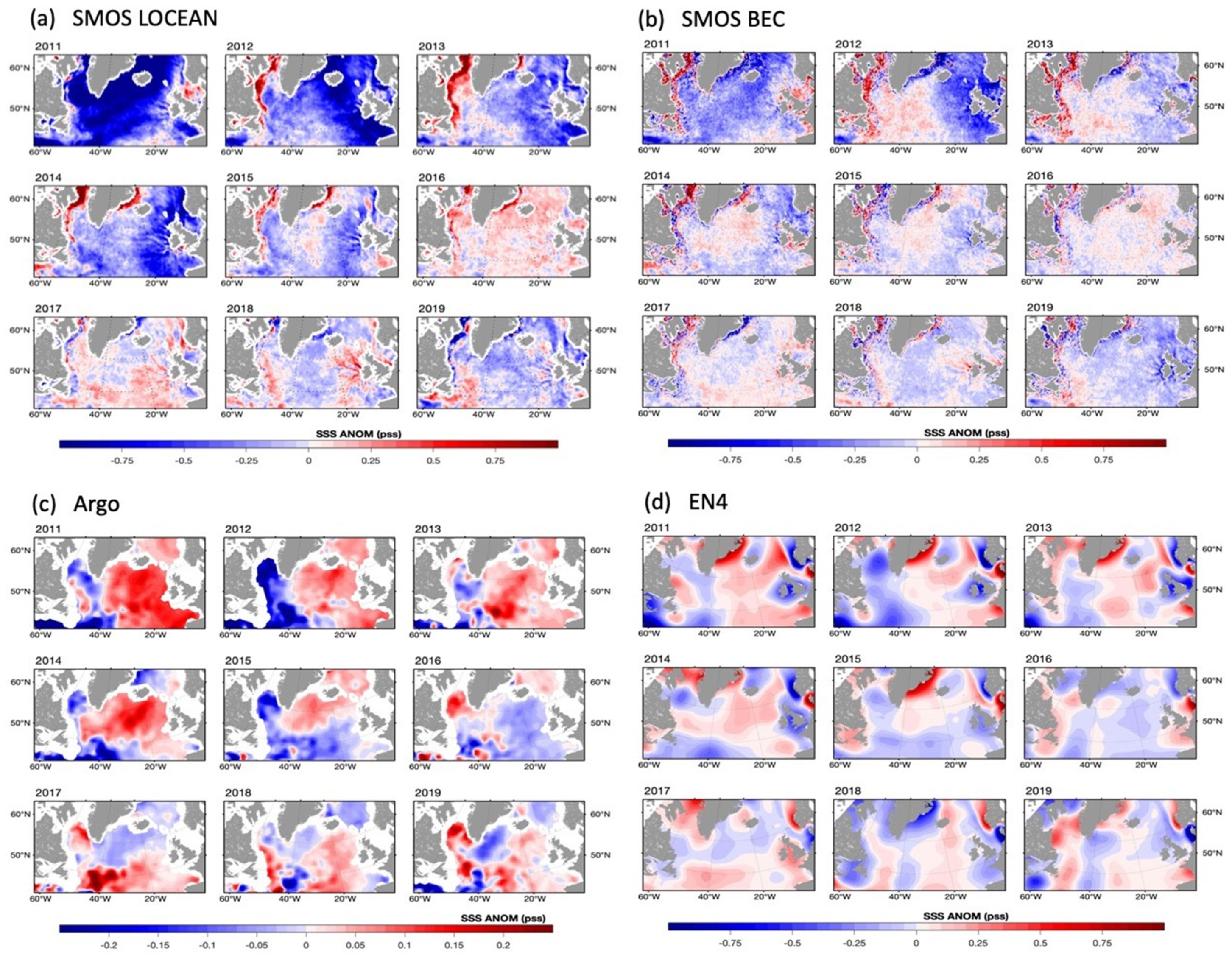
Sustained surface freshening anomalies from 2015 to 2016 were evidenced in Box 4 (NAC) in Argo and EN4, though not in SMOS LOCEAN or in SMOS BEC (Figure 10). The interannual time series of the two SMOS products did not reveal any significant SSS signal in 2012–2016, as the time series were contaminated by large drifts in early years and large interannual variability throughout the data record. To gain a better understanding of the basin-scale variability of SSS in SMOS products during the recent decade, yearly mean anomaly fields were constructed for SMOS, Argo, and EN4 in reference to the 2016–2018 mean (Figure 11).
SMOS LOCEAN had systematic drifts in the SPNA before 2015 (Figure 11a). The center location of the anomalies associated with the drift appeared to change with time: It occurred in the western-southwestern basin in 2011, in the eastern-southeastern basin in 2012–2013, and in the eastern basin in 2014–2015. Interestingly, SMOS BEC had a similar structure but with a much reduced magnitude (Figure 11b). The two SMOS products produced a basin-wide SSS increase in 2016 instead of surface freshening.
Unlike SMOS products, Argo and EN4 both yielded a significant, low SSS pattern in 2016 (Figure 11c–d). Evolution of the low salinity anomalies prior to and after 2016 suggested that the freshening event originated from the south and propagated north-northwestward along the NAC pathway. For instance, the year-to-year evaluation of the Argo SSS fields showed that fresh anomalies were first located near the Grand Banks of Newfoundland around 45°N, 40°W in 2011–2013. The freshening in the Newfoundland Basin expanded northward in the area influenced by the NAC in 2014–2015. Notably, in 2016, most of the basin south of Iceland was abnormally fresher while the Labrador Sea and the Nordic Seas were abnormally saltier. The fresh anomalies appeared in the Nordic Seas in 2017, causing the basin north of 50°N all to be very fresh. By 2018–2019, the surface freshening remained mostly in the Irminger Sea and the Nordic Seas. EN4 has a similar pattern for year-to-year evolution of SSS anomalies, though the structures were smoother. The study [5] was based on 50-year time series of EN4, while this study used EN4 during the SMOS period. Nevertheless, the basin-scale freshening event in 2015–2016 was so strong that it was easily identified from both the 50-year-long time series and the nine-year-long time series.
It seems that the drift in the early years of the SMOS record may not have been the only cause of the deviations of SMOS LOCEAN and BEC products from Argo and EN4. Examining the anomaly fields during the entire period of 2011–2019, one observes that yearly anomaly patterns agreed with Argo and EN4 only in partial areas for the two years, 2017–2018. During this period, the surface freshening in the Irminger Sea and Nordic Seas was captured by both SMOS and in situ products. The large departures between SMOS and in situ products indicated the need for enhanced validation and verification of SMOS SSS retrievals in the SPNA.
4. Discussion
Recent evaluation studies of satellite-derived SSS products in the subarctic and Arctic oceans [32,37,38,39,40,41] showed that satellite products had excellent consistency among one another in describing seasonal and interannual variations associated with the sea ice cycle. In particular, Arctic SSS had large spatiotemporal changes with magnitude often exceeding 3 pss, and, hence, the SSS retrievals of ~1 pss accuracy should be sufficient for detecting the large SSS changes induced by seasonal freshwater influx into the Arctic region [56]. This study found, however, that the four SMOS and SMAP products deviated considerably from each other and from in situ-based products in the subpolar North Atlantic for SSS variability on seasonal to interannual time scales. The findings seemed to indicate that satellite SSS products in the subpolar regions may not be as consistent as they are in the Arctic Ocean.
Harmonic analysis of annual and semiannual cycles revealed that satellite products all had difficulty producing the right annual cycle in the western basin, particularly the Labrador and Irminger seas, where the surface waters are colder and fresher. In situ products showed that the SSS in the Labrador Sea was saltier in winter and fresher in summer (Figure 5), but satellite products deviated considerably from this pattern in both amplitudes and phases. The Labrador and Irminger seas are a region of pronounced thermal and haline variability on interannual and decadal time scales and they play an important role in the North Atlantic Meridional Overturning Circulation (MOC) [13,14]. The inability of satellite products to produce the most basic climate signal emphasizes the need for enhanced efforts to improve and advance the retrieval skills in these regions.
The salinity in the Labrador and Irminger seas is strongly influenced by freshwater export from the Arctic Ocean, sea ice melting and freezing, and freshwater flux sourced from excessive precipitation over evaporation [7,8,9,10]. Several studies have investigated the key forcing in determining seasonal variability of SSS in the region. For instance, Schmidt and Send [57] examined the seasonal freshening of the Labrador Sea and found that it could not be attributed solely to local sources (e.g., precipitation-minus-evaporation (P–E), sea ice melting, and horizontal advection/mixing). They compared the timing and volume estimates of the seasonal freshwater cycles of the boundary currents with the salinity in the Labrador Sea, and suggested that 60%–80% of the annual freshwater in the central Labrador Sea originated from the WGC and the farther upstream EGC that carries the Arctic freshwater export, while only 20% is from precipitation. The ratio of the freshwater sources supports the results of ocean models [58] showing that the seasonal surface freshening in the Labrador Sea (and also the Irminger Sea) was largely controlled by freshwater export from the Arctic Ocean, in which the WGC plays a more important role than all other processes in transporting the Arctic freshwater.
Tang et al. [56] examined the year-to-year SSS variability in the Hudson Bay and also found that the main forcing of SSS variability was sea ice melting, not the surface P–E flux. They also pointed out that, though the freshwater contribution from P–E was small in magnitude compared with sea ice contribution, this surface freshwater input cannot be fully neglected as its accumulative impacts persist through the whole open water season and can affect SSS variability on seasonal and longer time scales. Overall, these studies indicate that, though basin integrals of surface P–E flux could be a useful proxy for SSS variability in the tropical and subtropical oceans [59,60], it is less predominant for SSS variability at higher latitudes. Useful proxies for validation and verification of satellite SSS retrievals at high-latitude, cold-water regions should be determined by local SSS dynamics and would vary from region to region.
5. Conclusions
This study evaluated two SMAP products (JPL and RSS) and two SMOS products (LOCEAN and BEC) in the SPNA with reference to two in situ, gridded products, Argo and EN4. Monthly mean fields were used in the evaluation, and the differences between satellite and in situ products in mean and variability of SSS during the period of 2011–2019 were examined. Major findings are summarized as follows.
Mean: Satellite products have a broad agreement with in situ products in the spatial distribution of time-mean SSS, with saltier surface waters in the eastern basin and fresher waters in the western marginal seas like the Labrador and Irminger seas. However, the magnitudes of mean SSS vary with products.
Seasonal variations: Annual and semiannual cycles were estimated using harmonic analysis. In situ products showed that the annual cycle dominates, with maximum SSS in March and minimum SSS in September, and the annual variations account for more than 91% of total seasonal variances. It was found that satellite products all had difficulty producing the right phases of the annual cycle, particularly in the marginal seas in the western basin. SMAP JPL and SMOS LOCEAN had major discrepancies, as they showed that the semiannual cycle is the predominant component and accounts for 61% and 78% of the seasonal variances, respectively.
Interannual variations: Both SMOS LOCEAN and BEC products had basin-scale, time-varying drifts before 2015, although SMOS BEC was biased with a lesser degree. The interannual anomalies deviated substantially from those of in situ products. In particular, in situ products indicated that the magnitudes of interannual SD were regime-dependent, larger in the fresher water regimes in the western basin and smaller in the saltier water regime in the eastern basin. None of these features were produced by SMOS LOCEAN and BEC.
Major freshening event in 2015–2016: The SPNA underwent a major freshening in 2015–2016 as revealed in in situ products and reported by recent studies [4,5]. This freshening event could not be identified in either SMOS LOCEAN or BEC because of the contamination of basin-wide biases in the products.
It is worth noting that the analysis in this study focused on the ice-free grid points in the products. Many efforts have been made by SMAP and SMOS data producers in improving SSS retrievals closer to the sea-ice edge. For instance, SMAP JPL retrieves SSS where sea ice concentration (SIC) is less than 3% [56], while SMAP RSS has a much lower SIC threshold [48], and SMOS LOCEAN uses a totally different platform and retrieval process [44]. There is an enhanced version of the Arctic SMOS SSS product developed through the specific ESA project Arctic+ Salinity at BEC [39]. The Arctic-centered SMOS product (poleward of 50°N) by BEC focused on capturing small-scale ocean dynamics using a modified interpolation scheme that can provide an effective resolution of 25 km. This analysis used the global SSS product by BEC.
To summarize, satellite SMAP and SMOS products in the subpolar regions need to be improved in the cold, fresh marginal seas in the western basin to ensure the correct production of seasonal cycles. Additionally, the basin-scale, time-varying drifts in the decade-long SMOS data record also need to be corrected before the datasets can be used for studying SSS variability on interannual and longer timescales. The progress made in the past 10 years has proven the capability of L-band remote sensing to measure SSS in the tropical to subtropical oceans. Improvements of the SSS retrievals in cold waters at mid-high latitudes will help further advance the full potential of salinity remote sensing from the tropical to the polar latitudes.
There are currently two new, exciting initiatives aiming to address the capability gap in salinity remote sensing in the polar and subpolar seas. One is the European Space Agency’s Copernicus Imaging Microwave Radiometer (CIMR) mission planned for the 2025+ timeframe. The CIMR mission is designed for an all-weather, high-spatial resolution, and accurate estimation of ocean and sea-ice surface parameters and more particularly the Arctic environment to support the Integrated Policy for the Arctic [61]. CIMR is a wide-swath, conically-scanning microwave radiometer that includes channels at 1.4, 6.9, 10.65, 18.7, and 36.5 GHz, also referred to as the L, C, X, Ku, and Ka bands. It promises to offer SST, SSS, and SIC measurements with a spatial resolution of 15, 55, and 5 km and a precision of 0.2 K, 0.3 pss, and 5%, respectively. By making simultaneous measurements at the five frequency bands with dual polarization, the CIMR mission will synergize and enhance the merits of the heritage missions including SMOS, SMAP, and advanced microwave scanning radiometer (AMSR) missions. The other initiative is NASA’s high-latitude salinity campaign that is planned in the 2022–2023 timeframe for three years [follow the link to access the program announcement]. The salinity-focused field study has specific science objectives that include linking salinity signatures to ice dynamics, learning about the Arctic freshwater balances from salinity information, and providing in situ support for enhancing salinity remote sensing [62]. Outcomes of these two initiatives will be a significant step forward for not only improving SSS remote sensing capabilities in cold waters, but also, more importantly, improving SSS applications for addressing the critical role of salinity in sea ice–ocean–atmosphere interactions in rapidly changing polar environments.
Funding
This research was funded by NASA Ocean Salinity Science Team (OSST) activities through Grant 80NSSC18K1335.
Acknowledgments
Review comments from two anonymous reviewers were appreciated. The author sincerely thanks the data producers for making satellite SSS datasets publicly available: the SMOS LOCEAN L3 Debiased products (https://www.catds.fr/Products/Available-products-from-CEC-OS/CEC-Locean-L3-Debiased-v4), the SMOS BEC global SSS products (http://bec.icm.csic.es/ocean-global-sss/), the SMAP JPL and RSS products (https://podaac.jpl.nasa.gov/SMAP). In situ gridded products were downloaded from these links: Argo (http://sio-argo.ucsd.edu/RG_Climatology.html) and EN4 (https://www.metoffice.gov.uk/hadobs/en4/).
Conflicts of Interest
The author declares no conflict of interest.
References
- Dickson, R.R.; Meincke, J.; Malmberg, S.A.; Lee, A.J. The “Great Salinity Anomaly” in the northern North Atlantic, 1968–1982. Progr. Oceanogr. 1988, 20, 103–151. [Google Scholar] [CrossRef]
- Curry, R.G.; Mauritzen, C. Dilution of the northern North Atlantic ocean in recent decades. Science 2005, 308, 1772–1774. [Google Scholar] [CrossRef] [PubMed] [Green Version]
- Friedman, A.R.; Reverdin, G.; Khodri, M.; Gastineau, G. A new record of Atlantic sea surface salinity from 1896 to 2013 reveals the signatures of climate variability and long-term trends. Geophys. Res. Lett. 2017, 44, 1866–1876. [Google Scholar] [CrossRef] [Green Version]
- Tesdal, J.E.; Abernathey, R.P.; Goes, J.I.; Gordon, A.L.; Haine, T.W. Salinity trends within the upper layers of the subpolar North Atlantic. J. Clim. 2018, 31, 2675–2698. [Google Scholar] [CrossRef]
- Holliday, N.P.; Bersch, M.; Berx, B.; Chafik, L.; Cunningham, S.; Florindo-López, C.; Hátún, H.; Johns, W.; Josey, S.A.; Larsen, K.M.H.; et al. Ocean circulation causes the largest freshening event for 120 years in eastern subpolar North Atlantic. Nat. Commun. 2020, 11, 585. [Google Scholar] [CrossRef] [PubMed]
- McCartney, M.S.; Talley, L.D. The Subpolar Mode Water of the North Atlantic. J. Phys. Oceanogr. 1982, 12, 1169–1188. [Google Scholar] [CrossRef] [Green Version]
- Walsh, J.E.; Portis, D.H. Variations of precipitation and evaporation over the North Atlantic Ocean, 1958–1997. J. Geophys. Res. 1999, 104, 16613–16631. [Google Scholar] [CrossRef] [Green Version]
- Josey, S.A.; Marsh, R. Surface freshwater flux variability and recent freshening of the North Atlantic in the eastern subpolar gyre. J Geophys. Res. 2005, 110, C05008. [Google Scholar] [CrossRef]
- Luo, H.; Castelao, R.M.; Rennermalm, A.K.; Tedesco, M.; Bracco, A.; Yager, P.L.; Mote, T.L. Oceanic transport of surface meltwater from the southern Greenland ice sheet. Nat. Geosci. 2016, 9, 528–532. [Google Scholar] [CrossRef]
- Sejr, M.K.; Stedmon, C.A.; Bendtsen, J.; Abermann, J.; Juul-Pedersen, T.; Mortensen, J.; Rysgaard, S. Evidence of local and regional freshening of Northeast Greenland coastal waters. Sci. Rep. 2017, 7, 13183. [Google Scholar] [CrossRef]
- Marshall, J.; Schott, F. Open-ocean convection: Observations, theory, and models. Rev. Geophys. 1999, 37, 1–64. [Google Scholar]
- Pickart, R.S.; Straneo, F.; Moore, G.W.K. Is Labrador Sea Water formed in the Irminger basin? Deep-Sea Res. Part I 2003, 50, 23–52. [Google Scholar] [CrossRef]
- Frankignoul, C.; Deshayes, J.; Curry, R. The role of salinity in the decadal variability of the North Atlantic meridional overturning circulation. Clim. Dyn. 2009, 33, 777–793. [Google Scholar] [CrossRef] [Green Version]
- Rhein, M.; Kieke, D.; Hüttl-Kabus, S.; Roessler, A.; Mertens, C.; Meissner, R.; Klein, B.; Böning, C.W.; Yashayaev, I. Deep water formation, the subpolar gyre, and the meridional overturning circulation in the subpolar North Atlantic. Deep Sea Res. Part II 2011, 58, 1819–1832. [Google Scholar] [CrossRef]
- Vinogradova, N.; Lee, T.; Boutin, J.; Drushka, K.; Fournier, S.; Sabia, R.; Stammer, D.; Bayler, E.; Reul, N.; Gordon, A.; et al. Satellite salinity observing system: Recent discoveries and the way forward. Front. Mar. Sci. 2019, 6, 243. [Google Scholar] [CrossRef]
- Kerr, Y.H.; Waldteufel, P.; Wigneron, J.-P.; Delwart, S.; Cabot, F.; Boutin, J.; Escorihuela, M.; Font, J.; Reul, N.; Gruhier, C.; et al. The SMOS L: New tool for monitoring key elements of the global water cycle. Proc. IEEE 2010, 98, 666–687. [Google Scholar] [CrossRef] [Green Version]
- Reul, N.; Grodsky, S.A.; Arias, M.; Boutin, J.; Catany, R.; Chapron, B.; d’Amico, F.; Dinnat, E.; Donlon, C.; Fore, A.; et al. Sea surface salinity estimates from spaceborne L-band radiometers: An overview of the first decade of observation (2010–2019). Remote Sens. Environ. 2020, 242, 111769. [Google Scholar] [CrossRef]
- Lagerloef, G.; Colomb, F.R.; Le Vine, D.; Wentz, F.; Yueh, S.; Ruf, C.; Lilly, J.; Gunn, J.; Chao, Y.I.; Decharon, A.; et al. The Aquarius/SAC-D mission—Designed to Meet the Salinity Remote Sensing Challenge. Oceanography 2008, 21, 68–81. [Google Scholar] [CrossRef] [Green Version]
- Le Vine, D.M.; Dinnat, E.P.; Meissner, T.; Wentz, F.J.; Kao, H.-Y.; Lagerloef, G.; Lee, T. Status of Aquarius and salinity continuity. Remote Sens. 2018, 10, 1585. [Google Scholar] [CrossRef] [Green Version]
- Entekhabi, D.; Njoku, E.G.; O’Neill, P.E.; Kellogg, K.H.; Crow, W.T.; Edelstein, W.N.; Entin, J.K.; Goodman, S.D.; Jackson, T.J.; Johnson, J.; et al. The soil moisture active passive (SMAP) mission. Proc. IEEE 2010, 98, 704–716. [Google Scholar] [CrossRef]
- Klein, L.A.; Swift, C.T. An improved model for the dielectric constant of sea water at microwave frequencies. IEEE J. Ocean. Eng. 1977, 2, 104–111. [Google Scholar] [CrossRef]
- Skou, N.; Hoffman-Bang, D. L-band radiometers measuring salinity from space: Atmospheric propagation effects. IEEE Trans. Geosci. Remote Sens. 2005, 43, 2210–2217. [Google Scholar] [CrossRef]
- Boutin, J.; Waldteufel, P.; Martin, N.; Caudal, G.; Dinnat, E. Salinity retrieved from SMOS measurements over Global Ocean: Imprecisions due to surface roughness and temperature uncertainties. J. Atmos. Ocean. Technol. 2004, 21, 1432–1447. [Google Scholar] [CrossRef]
- Le Vine, D.; Saji, A.; Kerr, Y.H.; Wilson, W.J.; Skou, N.; Sobjaerg, S. Comparison of model predictions with measurements of galactic background noise at L-band. IEEE Geosci. Remote Sens. 2005, 43, 2018–2023. [Google Scholar] [CrossRef]
- Dinnat, E.; Le Vine, D.; Boutin, J.; Meissner, T.; Lagerloef, G. Remote Sensing of Sea Surface Salinity: Comparison of Satellite and In Situ Observations and Impact of Retrieval Parameters. Remote Sens. 2019, 11, 750. [Google Scholar] [CrossRef] [Green Version]
- Reul, N.; Tenerelli, J.; Chapron, B.; Waldteufel, P. Modelling sun glitter at L-band for the sea surface salinity remote sensing with SMOS. IEEE Trans. Geosci. Remote Sens. 2007, 45, 2073–2087. [Google Scholar] [CrossRef]
- Oliva, R.; Daganzo, E.; Kerr, Y.H.; Mecklenburg, S.; Nieto, S.; Richaume, P.; Gruhier, C. SMOS radio frequency interference scenario: Status and actions taken to improve the RFI environment in the 1400–1427- MHz passive band. IEEE Trans. Geosci. Remote Sens. 2012, 50, 1427–1439. [Google Scholar] [CrossRef] [Green Version]
- Boutin, J.; Chao, Y.; Asher, W.E.; Delcroix, T.; Drucker, R.; Drushka, K.; Kolodziejczyk, N.; Lee, T.; Reul, N.; Reverdin, G.; et al. Satellite and in situ salinity: Understanding near-surface stratification and sub-footprint variability. Bull. Amer. Meteor. Soc. 2016, 97, 1391–1407. [Google Scholar] [CrossRef] [Green Version]
- Sutherland, D.; Pickart, R.S. The East Greenland Coastal Current: Structure, variability, and forcing. Prog. Oceanogr. 2008, 78, 58–77. [Google Scholar] [CrossRef] [Green Version]
- Myers, P.G.; Donnelly, C.; Ribergaard, M.H. Structure and variability of the west Greenland current in summer derived from 6 repeat standard sections. Prog. Oceanogr. 2009, 80, 93–112. [Google Scholar] [CrossRef]
- Meissner, T.; Wentz, F.; Le Vine, D. The salinity retrieval algorithms for the NASA Aquarius version 5 and SMAP version 3 releases. Remote Sens. 2018, 10, 1121. [Google Scholar] [CrossRef] [Green Version]
- Tang, W.; Yueh, S.; Yang, D.; Fore, A.; Hayashi, A.; Lee, T.; Fournier, S.; Holt, B. The potential and challenges of using Soil Moisture Active Passive (SMAP) sea surface salinity to monitor Arctic Ocean freshwater changes. Remote Sens. 2018, 10, 869. [Google Scholar] [CrossRef] [Green Version]
- Fore, A.G.; Yueh, S.H.; Tang, W.; Stiles, B.W.; Hayashi, A.K. Combined active/passive retrievals of ocean vector wind and sea surface salinity with SMAP. IEEE Trans. Geosci. Remote Sens. 2016, 54, 7396–7404. [Google Scholar] [CrossRef]
- Menezes, V.V. Statistical Assessment of Sea-Surface Salinity from SMAP: Arabian Sea, Bay of Bengal and a Promising Red Sea Application. Remote Sens. 2020, 12, 447. [Google Scholar] [CrossRef] [Green Version]
- Vazquez-Cuervo, J.; Gomez-Valdes, J.; Bouali, M.; Miranda, L.; Van der S/surnamtocken, T.; Tang, W.; Gentemann, C. Using Saildrones to Validate Satellite-Derived Sea Surface Salinity and Sea Surface Temperature along the California/Baja Coast. Remote Sens. 2019, 11, 1964. [Google Scholar] [CrossRef] [Green Version]
- Grodsky, S.A.; Vandemark, D.; Feng, H. Assessing coastal SMAP surface salinity accuracy and its application to monitoring Gulf of Maine circulation dynamics. Remote Sens. 2018, 10, 1232. [Google Scholar] [CrossRef] [Green Version]
- Köhler, J.; Martins, M.S.; Serra, N.; Stammer, D. Quality assessment of spaceborne sea surface salinity observations over the northern North Atlantic. J. Geophys. Res. Oceans 2015, 120, 94–112. [Google Scholar] [CrossRef] [Green Version]
- Garcia-Eidell, C.; Comiso, J.C.; Dinnat, E.; Brucker, L. Satellite observed salinity distributions at high latitudes in the Northern Hemisphere: A comparison of four products. J. Geophys. Res. Ocean 2017, 122, 7717–7736. [Google Scholar] [CrossRef] [Green Version]
- Olmedo, E.; Gabarró, C.; González-Gambau, V.; Martínez, J.; Ballabrera-Poy, J.; Turiel, A.; Portabella, M.; Fournier, S.; Lee, T. Seven years of SMOS sea surface salinity at high latitudes: Variability in Arctic and Sub-Arctic regions. Remote Sens. 2018, 10, 1772. [Google Scholar] [CrossRef] [Green Version]
- Xie, J.; Raj, R.P.; Bertino, L.; Samuelsen, A.; Wakamatsu, T. Evaluation of Arctic Ocean surface salinities from the Soil Moisture and Ocean Salinity (SMOS) mission against a regional reanalysis and in situ data. Ocean Sci. 2019, 15, 1191–1206. [Google Scholar] [CrossRef] [Green Version]
- Fournier, S.; Lee, T.; Tang, W.; Steele, M.; Olmedo, E. Evaluation and Intercomparison of SMOS, Aquarius, and SMAP Sea Surface Salinity Products in the Arctic Ocean. Remote Sens. 2019, 11, 3043. [Google Scholar] [CrossRef] [Green Version]
- Yueh, S.H.; Tang, W.; Hayashi, A.K.; Lagerloef, G.S.E. L-band passive and active microwave geophysical model functions of ocean surface winds and applications to aquarius retrieval. IEEE Trans. Geosci. Remote Sens. 2014, 51, 4619–4632. [Google Scholar] [CrossRef]
- Boutin, J.; Vergely, J.L.; Marchand, S.; D’Amico, F.; Hasson, A.; Kolodziejczyk, N.; Reul, N.; Reverdin, G.; Vialard, J. New SMOS sea surface salinity with reduced systematic errors and improved variability. Remote Sens. Environ. 2018, 214, 115–134. [Google Scholar] [CrossRef] [Green Version]
- Boutin, J.; Vergely, J.-L.; Thouvenin-Masson, C.; Supply, A.; Khvorostyanov, D. SMOS SSS L3 maps generated by CATDS CEC LOCEAN. debias V4.0. SEANOE 2019. [Google Scholar] [CrossRef]
- SMOS-BEC Team: Global SMOS-BEC Debiased non-Bayesian SSS L3 and L4 Product Description. Barcelona Expert Centre, Spain, Technical note: BEC-SMOS-0007-QR version 1.0. BEC 2019-07-15. Issue 1.0. p. 25. 2019. Available online: http://bec.icm.csic.es/doc/BEC-SMOS-0002-PD-SSS-Global.pdf (accessed on 15 May 2020).
- Olmedo, E.; Martínez, J.; Turiel, A.; Ballabrera-Poy, J.; Portabella, M. Debiased non-Bayesian retrieval: A novel approach to SMOS Sea Surface Salinity. Remote Sens. Environ. 2017, 193, 103–126. [Google Scholar] [CrossRef]
- Fore, A.; Yueh, S.; Tanh, W.; Hayashi, A. JPL SMAP Ocean Surface Salinity Products [Level 2B, Level 3 Running 8-day, Level 3 Monthly], Version 4.3 Validated Release; Jet Propulsion Laboratory: Pasadena, CA, USA, 2020. [CrossRef]
- Meissner, T.; Wentz, F.J.; Manaster, A.; Lindsley, R. Remote Sensing Systems SMAP Ocean Surface Salinities [Level 2C, Level 3 Running 8-day, Level 3 Monthly], Version 4.0 Validated Release; Remote Sensing Systems: Santa Rosa, CA, USA, 2019. [Google Scholar] [CrossRef]
- Roemmich, D.; Gilson, J. The 2004–2008 mean and annual cycle of temperature, salinity, and steric height in the global ocean from the Argo Program. Progr. Oceanogr. 2009, 82, 81–100. [Google Scholar] [CrossRef]
- Good, S.A.; Martin, M.J.; Rayner, N.A. EN4: Quality controlled ocean temperature and salinity profiles and monthly objective analyses with uncertainty estimates. J. Geophys. Res. Oceans 2013, 118, 6704–6716. [Google Scholar] [CrossRef]
- Swift, C.T. Passive microwave remote sensing. Bound.-Layer Meteor. 1980, 18, 25–54. [Google Scholar] [CrossRef]
- Yu, L. On Sea Surface Salinity Skin Effect Induced by Evaporation and Implications for Remote Sensing of Ocean Salinity. J. Phys. Oceanogr. 2010, 40, 85–102. [Google Scholar] [CrossRef]
- Wyrtki, K. The annual and semiannual variation of sea surface temperature in the North Pacific Ocean. Limnol. Oceanogr. 1965, 10, 307–313. [Google Scholar] [CrossRef]
- Bingham, F.M.; Foltz, G.R.; McPhaden, M.J. Seasonal cycles of surface layer salinity in the Pacific Ocean. Ocean Sci. 2010, 6, 775–787. [Google Scholar] [CrossRef] [Green Version]
- Melnichenko, O.V.; Hacker, P.; Bingham, F.; Lee, T. Patterns of SSS variability in the eastern tropical Pacific: Intra-seasonal to inter-annual time-scales from seven years of NASA satellite data. Oceanography 2019, 32, 20–29. [Google Scholar] [CrossRef]
- Tang, W.; Yueh, S.H.; Yang, D.; Mcleod, E.; Fore, A.; Hayashi, A.; Olmedo, E.; Martínez, J.; Gabarró, C. The Potential of Space-Based Sea Surface Salinity on Monitoring the Hudson Bay Freshwater Cycle. Remote Sens. 2020, 12, 873. [Google Scholar] [CrossRef] [Green Version]
- Schmidt, S.; Send, U. Origin and Composition of Seasonal Labrador Sea Freshwater. J. Phys. Oceanogr. 2007, 37, 1445–1454. [Google Scholar] [CrossRef] [Green Version]
- Myers, P.G. Impact of freshwater from the Canadian Arctic Archipelago on Labrador Sea Water formation. Geophys. Res. Lett. 2005, 32, L06605. [Google Scholar] [CrossRef]
- Vinogradova, N.; Ponte, R.M. Clarifying the link between surface salinity and freshwater fluxes on monthly to interannual time scales. J. Geophys. Res. Oceans 2013, 118, 3190–3201. [Google Scholar] [CrossRef]
- Yu, L. A global relationship between the ocean water cycle and near-surface salinity. J. Geophys. Res. 2011, 116, C10025. [Google Scholar] [CrossRef]
- Kilic, L.; Prigent, C.; Aires, F.; Boutin, J.; Heygster, G.; Tonboe, R.T.; Roquet, H.; Jimenez, C.; Donlon, C. Expected performances of the Copernicus Imaging Microwave Radiometer (CIMR) for an all-weather and high spatial resolution estimation of ocean and sea ice parameters. J. Geophys. Res. Oceans 2018, 123, 7564–7580. [Google Scholar] [CrossRef] [Green Version]
- Drushka, K.; Gaube, P.; Armitage, T.; Cerovecki, I.; Fenty, I.; Fournier, S.; Gentemann, C.; Girton, J.; Haumann, A.; Lee, T.; et al. A NASA high-latitude salinity campaign. Figshare J. Contrib. 2020. [Google Scholar] [CrossRef]
Figure 1.
(a) Bathymetry of the subpolar North Atlantic with names that are referred to in the text. The superimposed, colored arrows illustrate major surface currents (counterclockwise): Eastern Greenland Current (EGC), Western Greenland Current (WGC), Labrador Current (LC), North Atlantic Current (NAC), Irminger Current (IrC), and Norwegian Atlantic Current (NwAC). (b) Mean sea-surface temperature averaged over 2016–2018. Data are from SMAP Jet Propulsion Laboratory (JPL). The thick black line denotes the ice margin. The five boxed areas denote the areas selected for analysis in Figures 7–10.

Figure 2.
Monthly mean time series of (a) SMAP JPL, (b) SMAP RSS, (c) SMOS LOCEAN, (d) SMOS BEC, (e) Argo, and (f) EN4 for the available period of each data product during 2011–2019. Readers are referred to Section 2.1 and Section 2.2 for the definition of the abbreviated data product names. The time series were constructed from SSS averages over the permanent ice-free grids in the study area (65°W–10°N, 45–70°N).

Figure 3.
(a–f) Time-mean SSS patterns averaged over the three full years 2016–2018. (g–l) The difference anomaly fields referenced to the Argo mean SSS, (a,g) for SMAP JPL, (b,h) for SMAP RSS, (c,i) for SMOS LECEAN, (d,j) for SMOS BEC, (e,k) for Argo, and (f,l) for EN4.
Figure 3.
(a–f) Time-mean SSS patterns averaged over the three full years 2016–2018. (g–l) The difference anomaly fields referenced to the Argo mean SSS, (a,g) for SMAP JPL, (b,h) for SMAP RSS, (c,i) for SMOS LECEAN, (d,j) for SMOS BEC, (e,k) for Argo, and (f,l) for EN4.

Figure 4.
The standard deviation with respect to the time-mean SSS for the period of 2016–2018 in (a–f), for the SMAP period from May 2015 to December 2019 in (g–h), and for the SMOS period from January 2011 to December 2019 in (i–l). The product name is listed at the top of each frame.
Figure 4.
The standard deviation with respect to the time-mean SSS for the period of 2016–2018 in (a–f), for the SMAP period from May 2015 to December 2019 in (g–h), and for the SMOS period from January 2011 to December 2019 in (i–l). The product name is listed at the top of each frame.

Figure 5.
Amplitudes (a–f) and phases (g–l) of the annual SSS cycle for all six products.

Figure 6.
(a–f) and phases (g–l) of the annual SSS cycle for the semiannual SSS cycle for all six products.
Figure 6.
(a–f) and phases (g–l) of the annual SSS cycle for the semiannual SSS cycle for all six products.

Figure 7.
The estimated annual cycles averaged over the five selected boxed areas depicted in Figure 1b and the entire basin. (a) Box 1. LS: The Labrador Sea. (b) Box 2. IS: The Irminger Sea. (c) Box 3. NS: The Nordic Seas. (d) Box 4. SPG: The Subpolar Gyre. (e) Box 5. NFL: Newfoundland. (f) The entire subpolar North Atlantic basin.

Figure 8.
The the estimated semiannual cycles averaged over the five selected boxed areas depicted in Figure 1b and the entire basin. (a) Box 1. LS: The Labrador Sea. (b) Box 2. IS: The Irminger Sea. (c) Box 3. NS: The Nordic Seas. (d) Box 4. SPG: The Subpolar Gyre. (e) Box 5. NFL: Newfoundland. (f) The entire subpolar North Atlantic basin.

Figure 9.
The seasonal variations (i.e., the combination of the annual and semiannual cycles). averaged over the five selected boxed areas depicted in Figure 1b and the entire basin. (a) Box 1. LS: The Labrador Sea. (b) Box 2. IS:The Irminger Sea. (c) Box 3. NS: The Nordic Seas. (d) Box 4. SPG: The Subpolar Gyre. (e) Box 5. NFL: Newfoundland. (f) The entire subpolar North Atlantic basin.

Figure 10.
Monthly mean time series of SSS anomalies at the five boxed areas (a–e) and over the SPNA (f) during 2011–2019 for four products, SMOS LOCEAN, SMOS BEC, Argo, and EN4. The anomalies are referenced to the combined annual and semiannual modes of the harmonic analysis of the 2016–2018 period.

Figure 11.
Year-to-year variations of the yearly mean SSS anomalies produced by (a) SMOS LOCEAN, (b) SMOS BEC, (c) Argo, and (d) EN4. The anomalies are referenced to the 2016–2018 mean. Note that the color scale ranges from -1 to 1 pss in (a,b,d) but is reduced to –0.25 to 0.25 pss in (c).
Figure 11.
Year-to-year variations of the yearly mean SSS anomalies produced by (a) SMOS LOCEAN, (b) SMOS BEC, (c) Argo, and (d) EN4. The anomalies are referenced to the 2016–2018 mean. Note that the color scale ranges from -1 to 1 pss in (a,b,d) but is reduced to –0.25 to 0.25 pss in (c).


Table 1.
Parameters of the estimated annual, semiannual, and seasonal (annual + semiannual) variability for the period of 2016–2018. The parameters listed in the table include amplitude, timing of SSS maximum (denoted Smax), timing of SSS minimum (denoted Smin), and correlation coefficient with respect to Argo. The correlation coefficients in bold indicate that they were not statistically significant at the confidence interval of 95%.
| Product | SMAP JPL | SMAP RSS | SMOS LOCEAN | SMOS BEC | Argo | EN4 | |
|---|---|---|---|---|---|---|---|
| Mode of Variability | |||||||
| Annual | Amplitude (pss) | 0.04 | 0.06 | 0.03 | 0.1 | 0.07 | 0.19 |
| Timing of Smax | Dec | Mar | Jul | Feb | Mar | Mar | |
| Timing of Smin | Jun | Sept | Jan | Aug | Sept | Sept | |
| Corr. (wrt Argo) | 0.16 | 0.96 | −0.62 | 0.94 | − | 0.99 | |
| Semiannual | Amplitude (pss) | 0.06 | 0.01 | 0.05 | 0.03 | 0.02 | 0.05 |
| Timing of Smax | Jun., Dec. | Jun., Dec. | Jun., Dec. | Jun., Dec. | May, Nov. | May, Nov. | |
| Timing of Smin | Mar., Sept. | Mar., Sept. | Mar., Sept. | Mar., Sept. | Feb., Aug. | Feb., Aug. | |
| Corr. (wrt Argo) | 0.99 | 0.52 | 0.97 | 0.94 | − | 0.98 | |
| Seasonal | Smax (pss) | 0.10 | 0.06 | 0.08 | 0.08 | 0.06 | 0.16 |
| Smin (pss) | −0.08 | −0.07 | −0.07 | −0.12 | −0.08 | −0.24 | |
| Timing of Smax | Dec., May | Mar. | Jun., Nov. | Jan. | Apr. | Apr. | |
| Timing of Smin | Aug., Mar. | Sept. | Mar., Sept. | Sept. | Sept. | Sept. | |
| Corr. (wrt Argo) | 0.34 | 0.93 | −0.02 | 0.93 | − | 0.99 |
Table 2.
Percentage of SSS variances in the SPNA that can be explained by the annual, semiannual, and seasonal (annual + semiannual) variability.
Table 2.
Percentage of SSS variances in the SPNA that can be explained by the annual, semiannual, and seasonal (annual + semiannual) variability.
| Product | SMAP JPL | SMAP RSS | SMOS LOCEAN | SMOS BEC | Argo | EN4 | |
|---|---|---|---|---|---|---|---|
| Mode of Variability | |||||||
| Annual | 35 | 78 | 13 | 87 | 91 | 93 | |
| Semiannual | 61 | 10 | 78 | 12 | 7 | 6 | |
| Seasonal (Annual + Semiannual) | 96 | 88 | 91 | 99 | 98 | 99 | |
Table 3.
SD and correlation of the time series of monthly mean SSS anomalies averaged over the five selected boxes and the entire SPNA basin for the period of 2013–2019. The data record for 2011–2012 was not included due to the large drift in SMOS products. The correlation coefficients in bold indicate that they were not statistically significant at the confidence interval of 95%.
| Product | SMOS LOCEAN | SMOS BEC | Argo | EN4 | |
|---|---|---|---|---|---|
| Properties | |||||
| STD (pss) | Box 1 (LS) | 0.17 | 0.06 | 0.11 | 0.13 |
| Box 2 (IrS) | 0.19 | 0.09 | 0.04 | 0.20 | |
| Box 3 (NS) | 0.26 | 0.12 | 0.05 | 0.07 | |
| Box 4 (NAC) | 0.26 | 0.10 | 0.06 | 0.07 | |
| Box 5 (GB) | 0.21 | 0.09 | 0.11 | 0.14 | |
| Basin average | 0.11 | 0.04 | 0.02 | 0.04 | |
| Corr. (wrt Argo) | Box 1 (LS) | 0.31 | 0.15 | − | 0.73 |
| Box 2 (IrS) | 0.30 | 0.51 | − | 0.61 | |
| Box 3 (NS) | 0.32 | 0.32 | − | 0.48 | |
| Box 4 (NAC) | −0.35 | 0.14 | − | 0.80 | |
| Box 5 (GB) | 0.34 | 0.36 | − | 0.79 | |
| Basin average | −0.23 | −0.27 | − | 0.52 |
© 2020 by the author. Licensee MDPI, Basel, Switzerland. This article is an open access article distributed under the terms and conditions of the Creative Commons Attribution (CC BY) license (http://creativecommons.org/licenses/by/4.0/).
Share and Cite
MDPI and ACS Style
Yu, L. Variability and Uncertainty of Satellite Sea Surface Salinity in the Subpolar North Atlantic (2010–2019). Remote Sens. 2020, 12, 2092. https://0-doi-org.brum.beds.ac.uk/10.3390/rs12132092
AMA Style
Yu L. Variability and Uncertainty of Satellite Sea Surface Salinity in the Subpolar North Atlantic (2010–2019). Remote Sensing. 2020; 12(13):2092. https://0-doi-org.brum.beds.ac.uk/10.3390/rs12132092
Chicago/Turabian StyleYu, Lisan. 2020. "Variability and Uncertainty of Satellite Sea Surface Salinity in the Subpolar North Atlantic (2010–2019)" Remote Sensing 12, no. 13: 2092. https://0-doi-org.brum.beds.ac.uk/10.3390/rs12132092
Note that from the first issue of 2016, this journal uses article numbers instead of page numbers. See further details here.