Stratifying Forest Overstory for Improving Effective LAI Estimation Based on Aerial Imagery and Discrete Laser Scanning Data

Abstract

Accurately mapping forest effective leaf area index (LAIe) at the landscape level is a crucial step to better simulate various ecological and physiological processes such as photosynthesis, respiration, transpiration, and precipitation interception. The LAIe products obtained from two-dimensional (2-D) remotely sensed optical imageries are usually biased due to their inability to identify the vertical forest structure and eliminate the effects of forest background (i.e., shrubs, grass, snow, and bare earth). In this study, we first stratified the forest overstory and background layers and generated a forest background mask layer based on the structural information implicitly contained within the aerial laser scanning (ALS) data. We improved the retrieval accuracy of LAIe by combining light detection and ranging (Lidar)-based three dimensional (3-D) structural and 2-D spectral information. Then, we obtained the improved final LAIe estimation result by masking the forest background pixels from the optical remotely sensed imageries. Our results showed that: (1) Removing forest background information could effectively (R² increase from 20% to 30%) improve the estimation accuracy of optical-based forest LAIe depending on forest structure characteristics. (2) The forest background in the forest stands with low canopy cover showed more apparent effects on LAIe estimation compared with the forest stands with a high canopy cover. (3) The combination of ALS and optical remotely sensed data could produce the best LAIe retrieval result effectively by removing the forest background information.

1. Introduction

Leaf area index (LAI), defined as one half of total green leaf surface area per unit horizontal ground surface area [1], is a crucial biophysical structural parameter for global climate change research [2,3]. The accurate estimation of forest canopy LAI at the landscape level is the premise and basis for better understanding the matter and energy cycles of terrestrial ecosystems and the spatiotemporal variations in solar radiations within or under a forest canopy [4,5,6,7]. Effective LAI (LAIe) is different from LAI, which considers the non-random distribution of foliage in the canopy. However, LAIe is usually used as a proxy of LAI because it is easier to obtain from the field-based instruments and remotely sensed data [8]. LAIe can be converted to LAI by the methods from previous studies [9,10,11]. The forest stand can be divided into overstory and background layers in the vertical dimension [12]. Forest background refers to all the materials below the forest canopy, including understory, leaf litter, grass, lichen, moss, rock, soil, snow, or their mixtures [13].

The conventional optical remotely sensed data receives mixed spectral signals from both forest overstory and background. In the meantime, the field-based measurement usually focuses on the forest overstory components for building statistical models and LAI product validation purposes [14]. This inconsistency leads to a significant error in the inversion results of a forest canopy LAI [15,16,17]. For example, one of the crucial reasons for the differences between the various global LAI products is the ignorance of different structures between forest overstory and background [14,18]. The statistical relationships between various vegetation indices (VIs) and field-based forest overstory LAI have been used as the standard method to map forest LAI using optical remotely sensed data widely. Some particular VIs, such as reduced simple ratio (RSR), soil adjusted vegetation index (SAVI), or corrected normalized difference vegetation index (NDVIc), are proposed to mitigate the effects of forest background on the reflectance of a forest canopy [19,20,21]. However, the VI-LAI empirical relationship tends to be saturated in a high-density forest canopy [22,23]. Moreover, many of the VIs that can mitigate background effects depend on the relative contributions of the background and overstory layer components, which differ along with sensor and sun angles [24] and cannot effectively separate the vertical structure information of tree-shrub-grass.

Multi-angle optical remotely sensed data combined with radiative transfer models have been used to overcome the effects of forest background and improve the accuracy of LAI inversion [25] in both North America and Northern Europe, respectively [13,26]. Moreover, Jiao et al. [27] used the long-term accumulated multi-angle imaging radiometer (MISR) data to obtain the monthly forest background reflectance of the global forest. Yang et al. [28] separated the overstory and understory LAIs of coniferous and deciduous broadleaf forests by combining a moderate resolution imaging system (MODIS) and MISR data at the global scale.

By obtaining the ratio of the forest background, the directional reflectance information obtained from multi-angle and multispectral remotely sensed data can eliminate the effects of forest background on forest LAI reversion. However, there still exist some problems and challenges as follows: (1) the spatial resolution of multi-angle optical satellite imageries usually are low; (2) few on-orbit multi-angle satellite data are available; (3) due to the increased travel path of solar radiation before reaching satellite sensors, the quality of data is usually affected by the air condition, especially by the clouds; and (4) the difficulties in taking into account topographic variations [13]. In addition, for the optical geometry model, the spatial distribution of trees is assumed to obey the Neyman distribution [29], and the tree crowns are approximated with simple geometric models such as cone, cylinder [30]. Therefore, the complex individual tree structure and their various spatial distribution patterns introduce errors to the estimation of four forest components (i.e., sunlit forest overstory, sunlit background, shaded forest overstory, and shaded background) proportions and forest canopy LAI, which are the basic parameters for the study of bidirectional reflectance distribution of a forest canopy. Optical remotely sensed data could not accurately describe the 3-D forest structure. Therefore, it is necessary to improve the accuracy of LAI estimation by a new method of accurately depicting the 3-D forest structure.

Light detection and ranging (Lidar) is an active remote sensing method that can directly capture 3-D forest structure information [31]. Many studies have applied Lidar to accurately obtain the 3-D forest structural metrics such as tree height, stand volume, and canopy closure [32,33]. The aerial laser scanning (ALS) data holds the capacity to penetrate through a forest canopy and great potential to improve the retrieval accuracy of LAI at the landscape or regional level [34]. There are two commonly used methods to retrieve forest LAI using ALS data. (1) Statistical-based method: One usually uses the empirical statistical relationships between ALS-based forest canopy height or crown volume and field-based LAI measurements for LAI inversion [35,36,37]. However, the fixed simple mathematical models are only feasible for a specific homogeneous forested area with uniform tree species [38]. (2) Beer’s law-based method: Various penetration indices based on the gap fraction theory of Beer’s law have been developed to estimate forest LAI using ALS data [38,39,40,41,42]. The ability to capture 3-D structure information allows overcoming the saturation problem resulting from the non-linear spectral responses of optical remotely sensed data to increasing forest LAI [43]. However, the varied footprint sizes and point densities will introduce uncertainties to estimating the forest gap fraction and LAI [34]. Most of the current studies usually set a specific height threshold to remove the effects of forest background on LAI estimation using ALS data. For example, Richardson, Moskal, and Kim [38] classified the points whose normalized heights were beyond 1.2 m as forest overstory. The simple threshold method does not work for forest stands with complex vertical structures and various tree species compositions. By fusing the ALS data capable of stratifying forest overstory from the background and spectral imageries with the ability to identify the vegetation and non-vegetation of forested area, one can effectively remove the effects of forest background on LAI retrieval. The usage of appropriate quantitative fusion of different data sources can benefit from each other to improve the final result of forest LAI. Some studies have successfully combined optical remotely sensed and ALS data to retrieve vegetation parameters such as forest aboveground biomass, basal area, species mixture, stem density, and volume [44,45,46]. However, most of the studies used a combination of different variables obtained from optical remotely sensed and ALS data without distinguishing the effect of the vertical forest structure of trees-shrub-grass on the parameter inversion.

Currently, few studies have quantitatively evaluated the effects of forest background on LAIe inversion by combining aerial spectral and laser scanning data. The spectral information recorded by single-angle optical remotely sensed data has limited ability to eliminate the effects of forest background effectively for LAIe retrieval purposes due to the inability to obtain forest 3-D structural information. Therefore, an effective method is needed to be developed to improve the retrieval accuracy of forest overstory LAIe by combining the aerial spectral and laser scanning data. The specific goals of this study were as follows:

(1)

develop an algorithm to stratify the forest overstory and background using ALS data;

(2)

investigate the effects of forest background of LAIe retrieval by combing the aerial spectral and laser scanning measurements;

(3)

compare and map the forest overstory LAIe at landscape level using different combinations of optical and Lidar data and evaluate their accuracy.

2. Materials and Methods

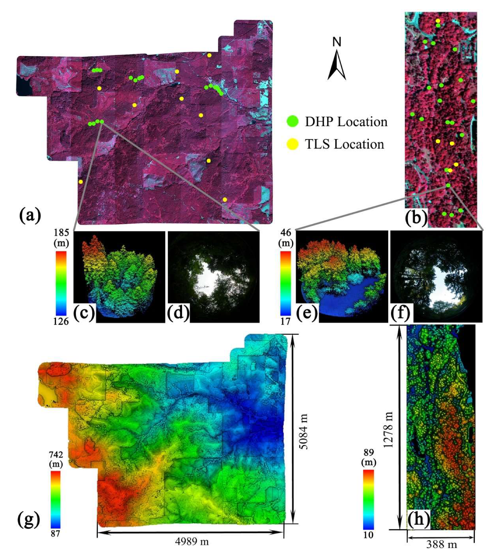
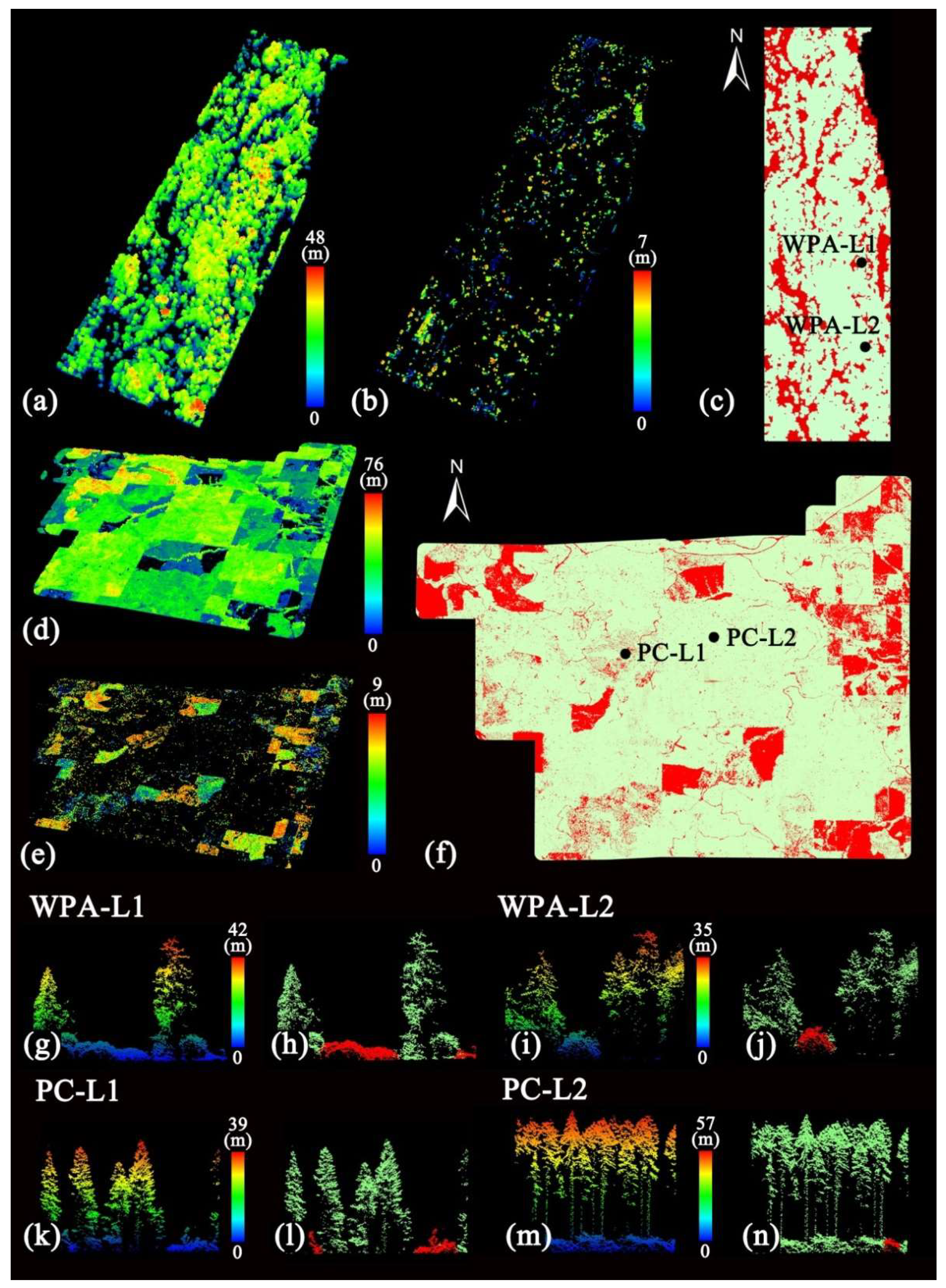
2.1. Study Area

There are two study areas in this study. The first one is the Washington Park Arboretum (WPA) (47.636°N, 122.296°W), covering an area of about 230 acres. It is located south of the University of Washington campus, Seattle, USA (Figure 1). More than 4600 species of vegetation were found from WPA, including trees, shrubs, and lianas. The Douglas fir (Pseudotsuga menziesii), Western hemlock (Tsuga heterophylla), Western red cedar (Thuja plicata), Big-leaf maple (Acer macrophyllum), Monkey puzzle (Araucaria araucana), Southern magnolia (Magnolia grandiflora), and New Mexican locust (Robinia neomexicana) are the dominant tree species of this study site. WPA is a managed urban forest with an elevation between 10 m and 48.47 m, and the terrain slope is less than 15°.

The second study site is Panther Creek (PC) (45.281°N, 123.368°W), located southeast of Portland, Oregon, USA. The total area of the PC is about 5580 acres (Figure 1). The dominant tree species include Western red cedar (Thuja plicata), Douglas fir (Pseudotsuga menziesii), Big-leaf maple (Acer macrophyllum), and Western hemlock (Tsuga heterophylla). PC is a natural forest with apparent topographic fluctuation. The elevation ranges from 87.32 m to 703.14 m, and the maximum terrain slope is 51.26°.

2.2. Datasets

2.2.1. Aerial Laser Scanning Data

The ALS data of WPA was obtained using the RIEGL LMS-Q560 laser scanner (Riegl, Co. Ltd., Horn, Austria) on 7 August 2008. The pulse frequency of the laser scanner was 133,000 Hz. The average flight altitude was about 310 m, while the lowest and highest flight altitudes were 145 m and 412 m, respectively. Multiple flight lines were designed to obtain point cloud data. The pulse emission density was about 10/m², and the scan zenith angle ranged from −30° to 30° from the nadir. The point cloud data was projected in UTM 10N, using WGS-84 ellipsoid datum, with units in meters. The ALS data of PC was acquired by the Leica ALS80 laser scanner (Leica Geosystems AG, Heerbrugg, Switzerland) on 18 June 2015, with a pulse frequency of 384,800 Hz. The average flight height was about 1400 m, and 24 east-west flight lines covered the study area. The pulse emission density was higher than 8/m², and the scan zenith angle ranged from −15° to 15°. The point cloud data was projected in Oregon Lambert, using the NAD83 (2011) horizontal datum and the NAVD88 (Geoid 12A) vertical datum, with units in international feet. The average point cloud densities of the WPA and PC study areas were 27 and 53 points/m².

2.2.2. Optical Spectral Data

A HyMap Sensor (HyVista Corporation, New South Wales, Australia) was used to obtain the aerial hyperspectral data of WPA on 15 August 2010. The hyperspectral imagery contained 128 bands, with a spectral range of 400–2500 nm and a spectral resolution of 15–16 nm (visible and near-infrared bands) and 15–20 nm (short-wave infrared bands). The spatial resolution of the aerial imagery was 2.9 m. The HyCorr software (HyVista Corporation, New South Wales, Australia) was used for radiative correction, and the known field control points were used for geometric correction. The coordinate system of the imagery was UTM 10N with the WGS84 datum. The hyperspectral data of the PC was obtained using the CASI-1500 sensor (ITRES Corporation, Calgary, Canada) from 3 to 5 September 2014. The imagery consisted of 96 bands with a spectral range of 380–1050 nm. The spectral resolution and spatial resolution were 3.6 nm and 0.5 m, respectively. We pre-processed the imagery using the ITRES (ITRES Corporation, Calgary, Canada) and ATCOR4 software (ReSe Applications LLC Corporation, Wil, Switzerland) for radiative correction and Inertial Explorer software (NovAtel Corporation, Calgary, Canada) for geometric correction. The coordinate system of the imagery was also set as the UTM 10N with the WGS84 datum.

2.2.3. Field-Based LAIe Measurements

• Digital Hemispherical Photos (DHP):

We used a digital camera (Nikon CoolPix 4500, Nikon Inc, Melville, NY, USA) equipped with a fisheye lens (Nikon Fisheye Converter FC-E8) to take hemispherical photos of 19 forest plots from 8 to 15 September 2008 in the WPA (Figure 1). At the same time, we used the Trimble GeoXT (Trimble Navigation Ltd., Sunnyvale, CA, USA) to record the geographic coordinates of the center point for each plot. The photos were processed by the Gap Light Analyzer (GLA Version 2.0) software [47]. GLA can calculate the LAIe of each forest plot by obtaining the forest gap fraction and other parameters (

Table 1. Forest plot characteristics in both the WPA and PC study areas.

Plot	Tree	Forest Type	Mean Height (m)	LAIe	Canopy Cover	Plot	Tree	Forest Type	Mean Height (m)	LAIe	Canopy Cover
WPA-1	13	C	25.74	3.66	0.41	PC-1	70	C	17.17	3.76	0.85
WPA-2	13	C	28.81	2.79	0.52	PC-2	63	C	17.05	3.74	0.85
WPA-3	16	M	26.24	2.16	0.83	PC-3	72	C	26.82	5.15	0.96
WPA-4	14	M	22.50	2.13	0.59	PC-4	51	C	26.42	4.20	0.90
WPA-5	11	M	22.73	3.18	0.48	PC-5	77	C	26.55	4.83	0.96
WPA-6	14	M	28.82	2.18	0.71	PC-6	34	C	27.41	2.37	0.88
WPA-7	16	C	24.02	1.45	0.63	PC-7	33	C	25.23	3.28	0.83
WPA-8	18	M	21.18	2.06	0.54	PC-8	29	C	25.97	3.64	0.69
WPA-9	14	M	21.96	1.58	0.64	PC-9	47	C	23.24	3.24	0.89
WPA-10	14	B	26.16	1.47	0.73	PC-10	39	C	23.94	3.92	0.88
WPA-11	16	C	24.16	2.12	0.76	PC-11	25	C	37.66	3.95	0.81
WPA-12	17	M	23.77	2.67	0.76	PC-12	32	C	37.94	4.71	0.82
WPA-13	19	B	18.20	3.42	0.70	PC-13	33	C	39.64	4.66	0.83
WPA-14	21	C	23.78	2.56	0.78	PC-14	28	C	38.02	4.25	0.84
WPA-15	23	C	26.51	3.37	0.84	PC-15	36	C	41.16	3.45	0.96
WPA-16	7	C	26.64	0.96	0.47	PC-16	68	C	28.24	5.38	0.98
WPA-17	16	C	22.55	1.87	0.84	PC-17	52	C	33.06	4.26	0.98
WPA-18	26	M	22.59	3.58	0.92	PC-18	34	C	39.20	4.44	0.88
WPA-19	19	M	19.64	2.37	0.64	PC-19	35	C	40.52	4.97	0.78
WPA-V1	18	M	20.68	2.29	0.72	PC-20	80	C	20.52	5.34	0.98
WPA-V2	24	B	29.40	3.71	0.90	PC-V1	39	C	39.39	2.89	0.92
WPA-V3	27	M	32.12	4.11	0.94	PC-V2	35	C	47.93	3.53	0.95
WPA-V4	21	M	30.64	3.04	0.93	PC-V3	78	C	16.75	4.06	0.84
WPA-V5	17	B	26.53	3.66	0.87	PC-V4	41	C	25.12	4.25	0.89
Mean	17	−	24.95	2.60	0.71	PC-V5	60	C	25.93	5.14	0.93
						PC-V6	52	C	31.79	5.16	0.82
						Mean	48	-	28.11	4.18	0.88

(Note: C: Conifer; B: Broadleaf; M: Mixed).

). We used the same instruments to obtain the LAIe values and center location coordinates of 17 forest plots from 20 to 28 June 2015 in the PC study area (Table 1). To eliminate the influence of topography, we used an LAI 4 ring value integrated from zenith angles of 0°–60° to process the DHP from WPA and PC sites. The mean LAI values were used as the representative values of the forest plots.

• Terrestrial Laser Scanning (TLS) data:

In September 2008 and July 2011, we used the Leica Scanstation II (Leica Geosystem AG, St. Gallen, Switzerland) to obtain the single station TLS point cloud data of 5 WPA plots and 9 PC plots, respectively. We scanned these plots using a hemispherical method (horizontal: 0° to 360°; vertical: −45° to 90°). Due to the various vegetation densities of each study site, we applied the sampling spacings of 2 cm @ 30 m and 1 cm @ 50 m to the plots of WPA and PC, respectively. Then, a radial hemisphere slice algorithm (RHSA) proposed by Zheng et al. [48] was used to process the TLS point cloud data. This algorithm projects a 3-D point cloud to a two-dimensional (2-D) hemispherical surface to simulate the way of calculating the LAIe by DHP. Therefore, the RHSA-based LAIe showed good agreement with the DHP-based ones [48]. In the projection of point cloud, we set the angular resolutions of the zenith and azimuthal direction as 1–1.5 times that of the sampling spacing [49] and used the same field of view angle and ring number as DHP to calculate the LAIe. The results of the TLS-based LAIe are shown in Table 1.

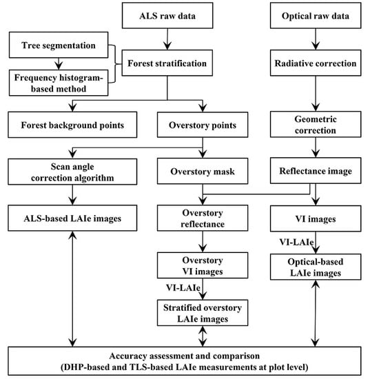
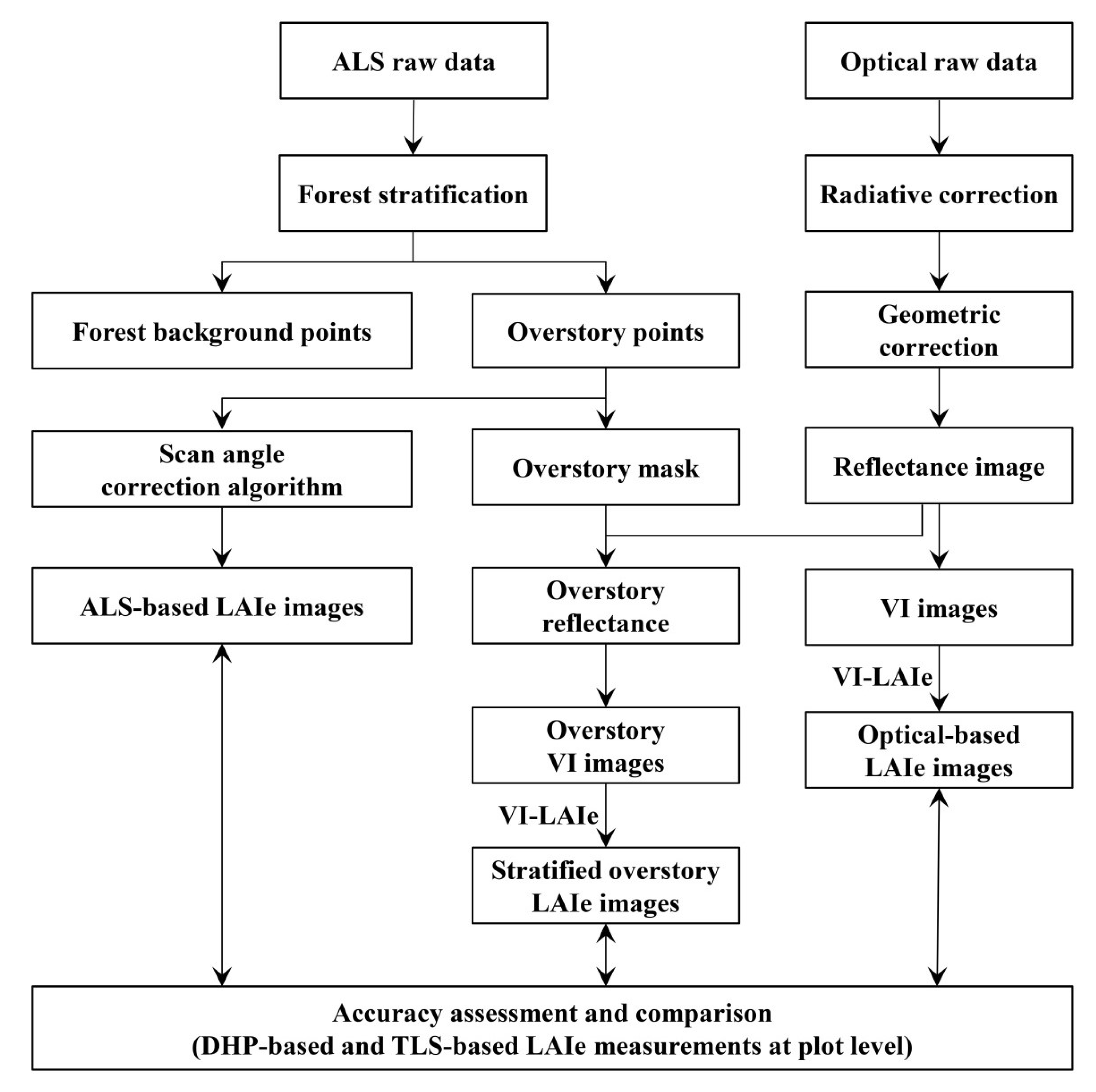
2.3. Overall Workflow

The overall flowchart of the study is shown in Figure 2. We first segmented the raw ALS data into individual trees and stratified forest overstory and background layers. Then, we masked the corresponding pre-processed optical spectral imageries to obtain the forest overstory layer. Based on the statistical relationship between the field-based LAIe and VIs of masked forest overstory, the final forest LAIe products were produced after removing the forest background by combining the aerial spectral and laser scanning data.

2.4. Tree Segmentation

We first used the CSF (Cloth Simulation Filter) algorithm [50] of the CloudCompare software (EDF, R&D. Paris, France) [51] to filter the ground points, and generated the digital terrain model (DTM) and normalized the forest heights using the FUSION software [52]. After grouping discrete points into individual tree crowns using the tree crown segmentation algorithm proposed by Li et al. [53], we obtained the tree height, crown size, and tree location information of each tree. The tree crown segmentation algorithm and extraction of tree parameters were realized by the C++ programming language.

The tree crown segmentation algorithm is a top-to-bottom region growing approach based on the raw 3-D point cloud data. The minimum distance threshold (DT) and searching sphere radius (SSR) used to find the local maximum point are two key parameters. By comparing the segmentation results of forest plots with the changes in the DT and SSR from 1 to 4 m at 0.5 m intervals, we determined the DT and SSR as 3 m and 2 m for the WPA and PC sites, respectively.

To validate the tree crown segmentation results, we visually identified the treetop points and measured the crown size of each tree using the FUSION software in the forest plots from the WPA and PC sites. Based on the matching of automated treetop points and visual treetop points, we obtained the root mean squared error (RMSE) of the crown radius to evaluate the accuracy of the segmentation algorithm.

2.5. Forest Stratification

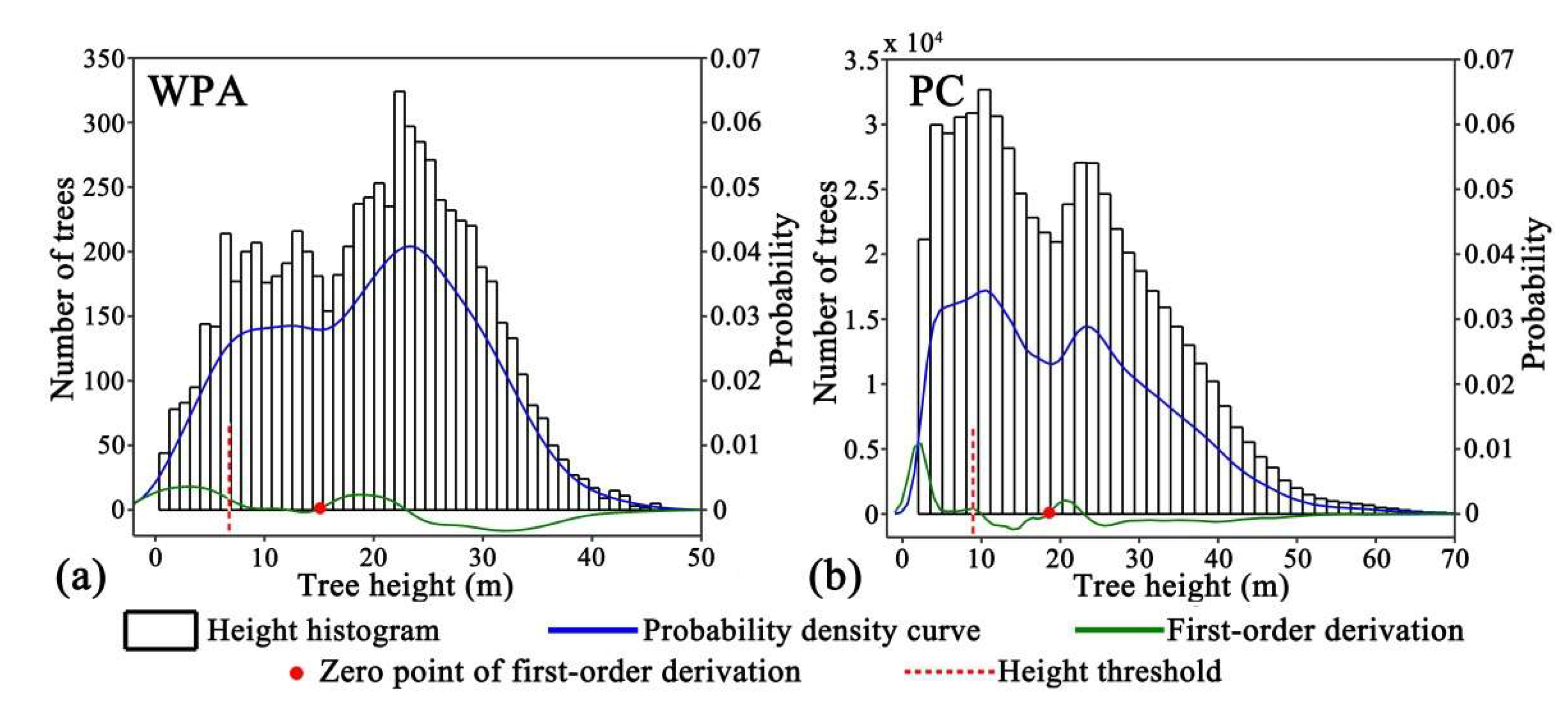
2.5.1. Height Threshold Determination

The tree height threshold was determined to stratify the forest overstory and background using the frequency histogram-based method (Figure 3). We first plotted the tree height frequency for the segmented tree crowns and obtained the double-peak probability density curves of the tree height distribution patterns in both the WPA and PC sites. By computing the first-order derivations of the tree height frequency curves, we determined the height stratification threshold as half of the tree height whose first-order derivative was zero and was the trough of the probability density curve (Figure 3).

2.5.2. Overstory Spectral Imagery

To remove the effects of the forest background on estimating the forest overstory LAIe, we generated a binary raster image based on the stratified ALS overstory points. The grid size was consistent with the pixel size of optical imageries for comparison purposes. Moreover, we converted the datasets into the same projections system (i.e., UTM 10 N). Then, based on the number of points in each grid, we reclassified the optical spectral imageries into a binary image by setting a threshold (T_num) for the number of points. The value of T_num was computed as (Equation (1)):

$$T_{num}=\frac{{Re}^{2}D}{4}$$

(1)

where $T_{num}$ is related to average point cloud density ($D$) and image spatial resolution ($Re$). We took T_num as 1/4 of the average number of points in each pixel. If the number of points in the cell was higher than T_num, it was assigned to 1; otherwise, it was assigned to 0. According to the average point cloud densities and the spatial resolutions of hyperspectral images in the study areas, we determined that the T_num of the WPA and PC study areas were 57 and 3, respectively. Finally, we obtained the forest overstory spectral imageries by masking out the forest background pixels using the ALS-based mask layer.

2.6. LAIe Mapping

2.6.1. Optical-Based LAIe

We selected 24 and 26 circular forest plots with a radius of 30 m in both the WPA and PC sites in September 2008 and June 2015, respectively (Figure 1). Among these forest plots, we built linear regression statistical models between the normalized difference vegetation index (NDVI) and simple ratio (SR) and field-based LAIe values using 19 (i.e., forest plot WPA-1~WPA-19) and 20 (i.e., forest plot PC-1~PC-20) plots for the WPA and PC sites. The rest of the forest plots (i.e., forest plot WPA-V1~WPA-V5 and PC-V1~PC-V6) were used for the validation purposes of the final LAIe product. Finally, we applied the statistical relationships between NDVI and LAIe to map the optical-based LAIe in both the WPA and PC sites.

2.6.2. ALS-Based LAIe

We obtained the ALS-based LAIe values of the forest plots (i.e., forest plot WPA-1~WPA-19 and PC-1~PC-20) using a scan angle correction algorithm (SACA)-based approach [54]. To compare with optical-based LAIe, we established linear regression statistical models between the ALS-based and field-based LAIe values using these forest plots in the WPA and PC sites. By dividing the the ALS overstory data of the WPA and PC sites into square grids with the side length of 10 m, we used the SACA-based approach to calculate the LAIe of each grid and generated the ALS-based LAIe maps with a spatial resolution of 10 m in both the WPA and PC sites finally. The choice of 10 m represents a tradeoff between retaining the spatial details and suppressing the wrong LAIe values due to insufficient scan angle information.

The SACA-based approach employed the Beer’s law to obtain the LAIe by calculating the gap fraction and the extinction coefficient. Voxel size is a crucial factor in estimating the gap fraction of a point cloud. According to the voxel size sensitivity analysis method [54], we chose 0.5 and 1.2 m as the voxel size of the WPA and PC sites.

2.6.3. Stratified Forest Overstory LAIe

We used the same forest plots (i.e., forest plot WPA-1~WPA-19 and PC-1~PC-20), as described in Section 2.6.1, to establish the linear regression statistical models between the VIs (i.e., NDVI and SR) from stratified overstory spectral imageries and the field-based LAIe values in the WPA and PC sites. Moreover, we still used the forest plots WPA-V1~WPA-V5 and PC-V1~PC-V6 as the verification plots. Finally, we applied the statistical relationships between NDVI and LAIe to map the stratified forest overstory LAIe in both the WPA and PC sites to assess the effects of the forest background on the LAIe estimation.

3. Results

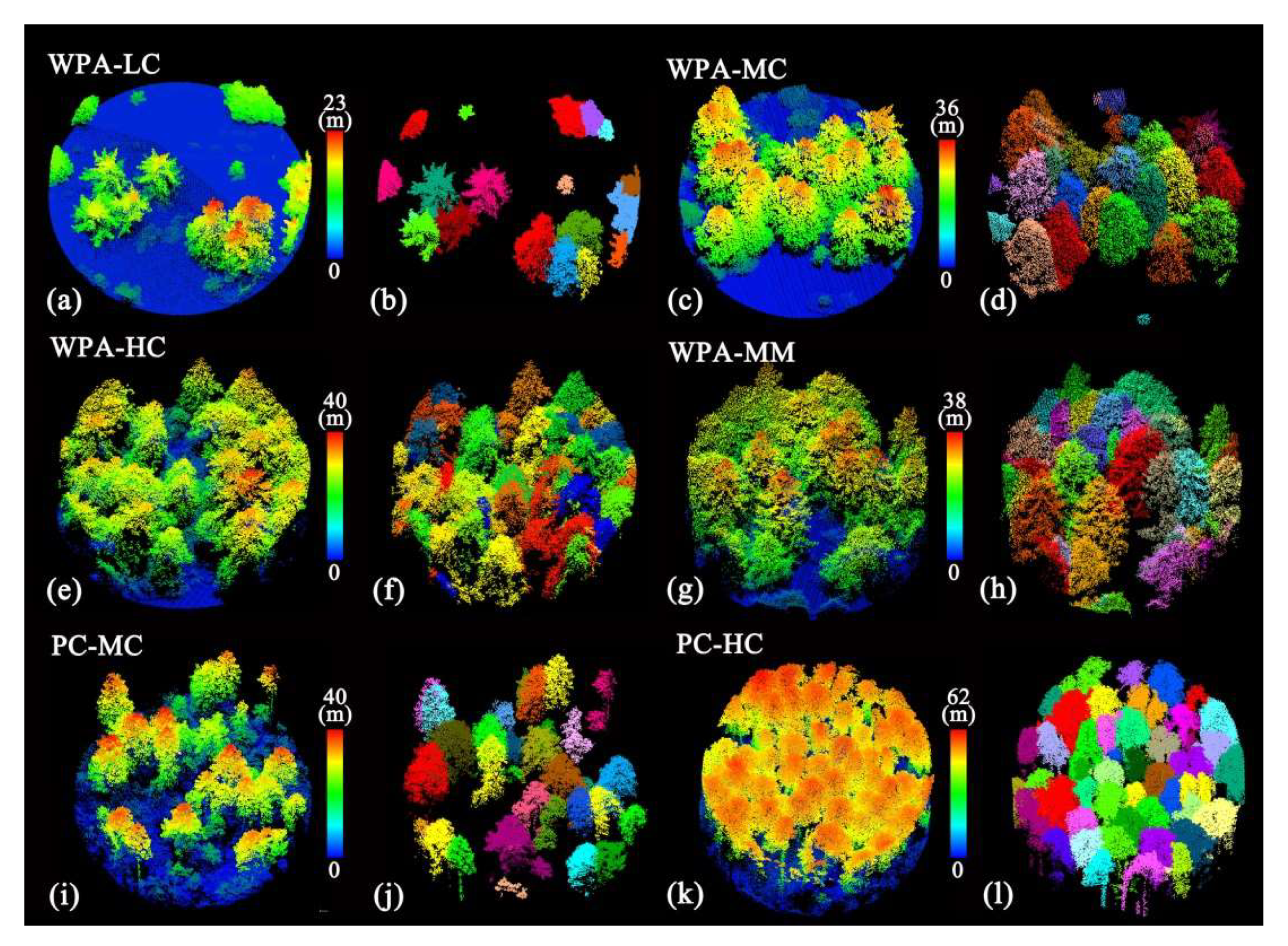
3.1. Tree Segmentation Results and Validation

We obtained the tree segmentation results for six circular test plots with different densities (high, medium, and low) and forest types (coniferous forest and mixed forest) with a radius of 30 m from the WPA and PC sites, including the WPA-LC (Figure 4a,b), WPA-MC (Figure 4c,d), WPA-HC (Figure 4e,f), WPA-MM (Figure 4g,h), PC-MC (Figure 4i,j), and PC-HC (Figure 4k,l), respectively.

Table 2. Accuracy evaluation of tree segmentation for the forest plots in both the WPA and PC sites.

Plot	Density	Tree #	Forest Type	Segmented Tree #	TP	FP	FN	Crown Radius RMSE (m)
WPA-LC	Low	10	C	11	10	1	0	0.45
WPA-MC	Medium	17	C	18	17	2	0	0.94
WPA-HC	High	24	C	26	23	3	1	1.37
WPA-MM	Medium	18	M	19	16	3	3	1.82
PC-MC	Medium	30	C	29	28	2	2	1.16
PC-HC	High	52	C	45	44	1	7	2.15
Overall	-	151	-	148	138	10	13	1.63

Note: C: conifer; M: mixed; TP: perfect segmentation; FP: over-segmentation; FN: under-segmentation.

is the tree segmentation verification results of these forest plots, where TP (true positive), FN (false negative), and FP (false positive) represent perfect segmentation, under-segmentation, and over-segmentation, respectively. The result shown that the tree crown segmentation algorithm detected 138 trees from the 151 trees of the six test plots, and the overall crown radius RMSE was 1.63 m. With the increase in forest plots densities, the number of falsely segmented (i.e., over-segmented and under-segmented) trees and crown radius RMSEs increased in both the WPA and PC sites. The crown radius RMSEs increased from 0.45 to 1.37 m, and the number of falsely segmented trees increased from 1 to 4 in the three low-, medium-, and high-density coniferous forest plots of the WPA sites. The crown radius RMSEs increased from 1.16 to 2.15 m, and the number of falsely segmented trees increased from 4 to 8 in the two medium- and high-density coniferous forest plots of the PC sites. Moreover, the crown radius RMSE of a mixed forest plot (i.e., WPA-MM) was higher than the RMSE of a coniferous forest plot (i.e., WPA-MC) with the same density.

3.2. Forest Stratification Result and Validation

The stratified height thresholds of the WPA and PC sites obtained by the frequency histogram-based method were 7 m and 9 m, respectively (Figure 3). We visualized the results of the forest overstory points (Figure 5a,d), understory points (Figure 5b,e), and binary images (Figure 5c,f) in both the WPA and PC sites. To show the details, we obtained the forest stratification results for four east-west line transects with a length of 60m from the WPA and PC sites, including the WPA-L1 (Figure 5g,h), WPA-L2 (Figure 5i,j), PC-L1 (Figure 5k,l), and PC-L2 (Figure 5m,n), respectively. The results show that the stratification method could effectively separate the vegetation below the gap between the crowns in the middle- and low-density forest. However, in the high-density forest, this ability was weakened due to the occlusion of tree crowns. Moreover, we obtained the canopy cover by calculating the proportion of the overstory area to the total area of a forest plot from the ALS data of six test forest plots (

Table 3. The verification of the forest stratification results.

Plot	Canopy Cover	P	D (%)	P(0)	D(0) (%)
WPA-LC	0.20	0.19	−1	0.35	15
WPA-MC	0.53	0.54	1	0.70	17
WPA-HC	0.65	0.70	5	0.87	22
WPA-MM	0.54	0.51	−3	0.83	29
PC-MC	0.43	0.42	−1	0.47	4
PC-HC	0.83	0.82	−1	0.87	4

). The overstory proportions of a forest plot (P) was computed as the ratio of the number of overstory pixels over the total number of pixels in a stratified forest plot image. The result showed that the differences (D) between the P and canopy cover were both less than 5% in the four forest plots with different densities and forest types from the WPA site. For the two medium- and high-density forest plots from the PC site, the D values were both −1%.

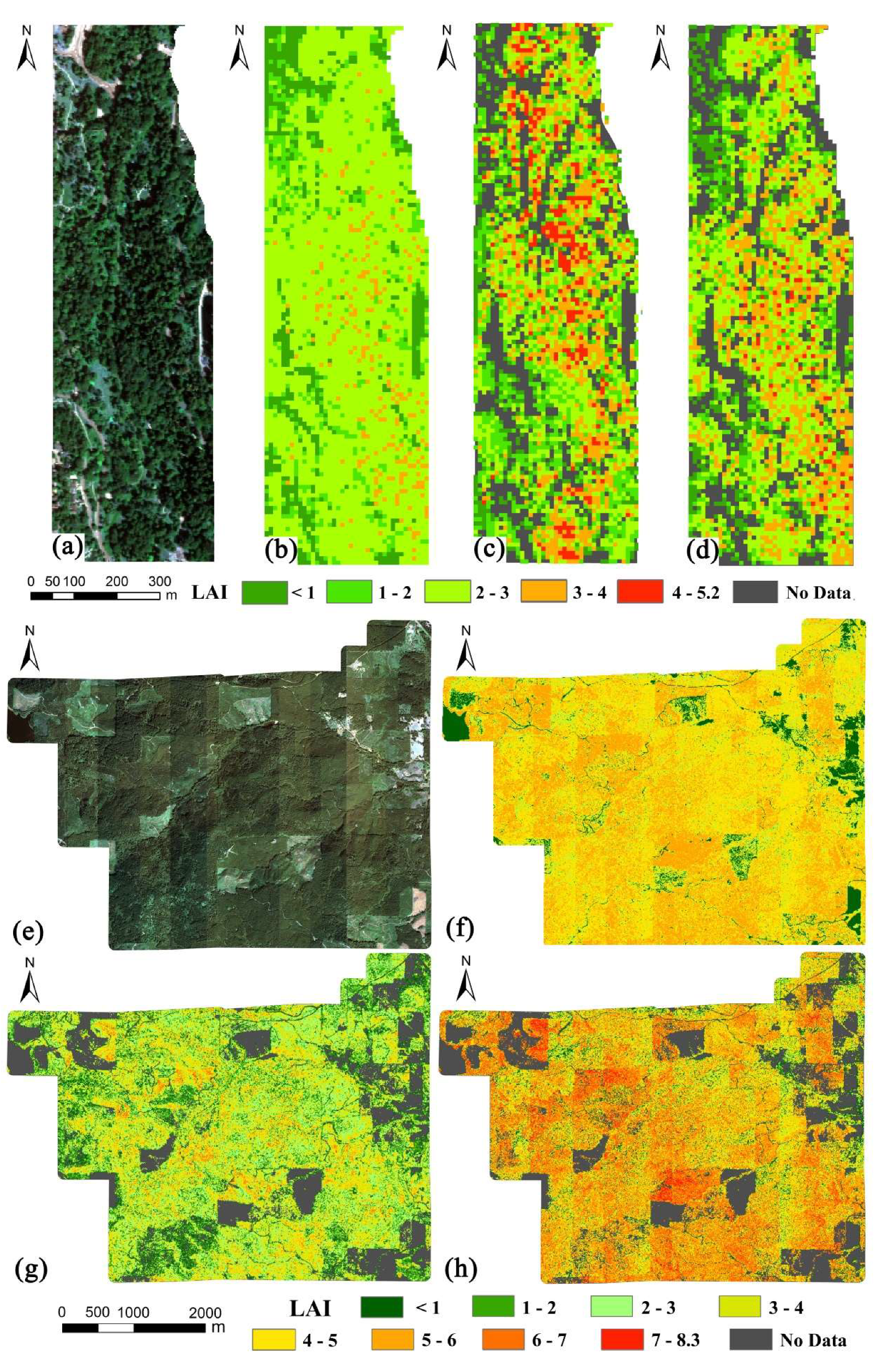
3.3. LAIe Mapping Results and Validation

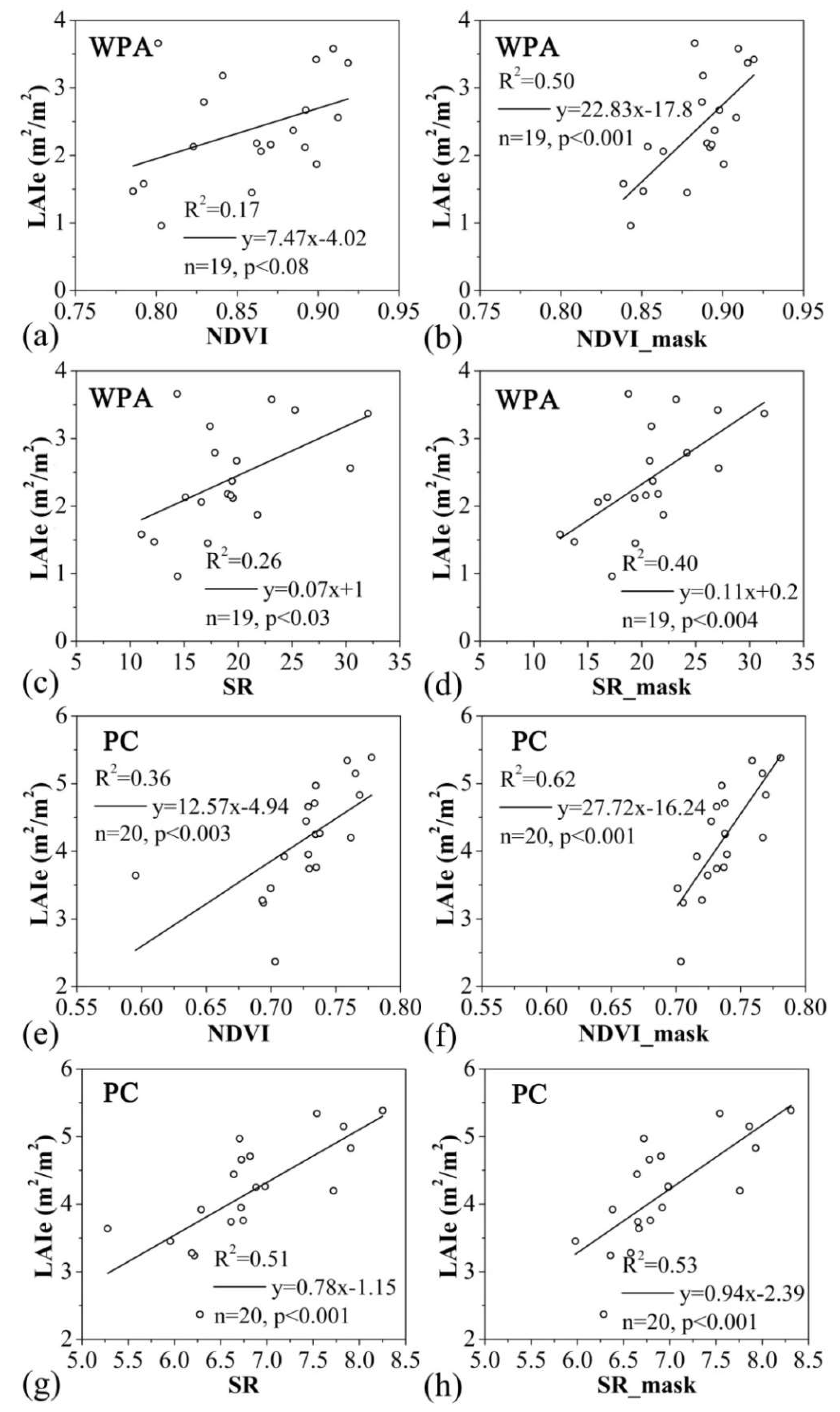
3.3.1. Optical-Based LAIe

We built linear regression statistical models between the NDVI and SR and field-based LAIe values (i.e., NDVI-LAIe and SR-LAIe) using optical imageries in the WPA (Figure 6a,c) and PC (Figure 6e,g) sites. We found that the R² values of NDVI-LAIe were lower than the corresponding R² values of SR-LAIe in both the WPA and PC sites. To compare the LAIe products from different data, we generated optical-based LAIe maps and increased their spatial resolution to 10 m in the WPA (Figure 7b) and PC (Figure 7f) sites. The verification results (

Table 4. Validation of the LAIe maps in both the WPA and PC sites.

Study Area	Plot	Field-Based LAIe	Optical-Based LAIe	ALS-Based LAIe	Stratified Forest Overstory LAIe
WPA	WPA-V1	2.29	2.67	2.28	2.61
	WPA-V2	3.71	2.76	2.75	2.95
	WPA-V3	4.11	2.80	3.63	3.05
	WPA-V4	3.04	2.71	2.61	2.81
	WPA-V5	3.66	2.51	2.14	2.64
	RMSE	-	0.92	0.85	0.76
PC	PC-V1	2.89	3.87	2.43	3.23
	PC-V2	3.53	4.29	2.12	4.15
	PC-V3	4.06	4.25	2.79	4.09
	PC-V4	4.25	3.99	2.98	3.52
	PC-V5	5.14	4.78	3.54	5.21
	PC-V6	5.16	4.68	4.06	5.04
	RMSE	-	0.58	1.24	0.42

) showed that the RMSEs of the optical-based LAIe maps were 0.92 and 0.58 in both the WPA and PC sites.

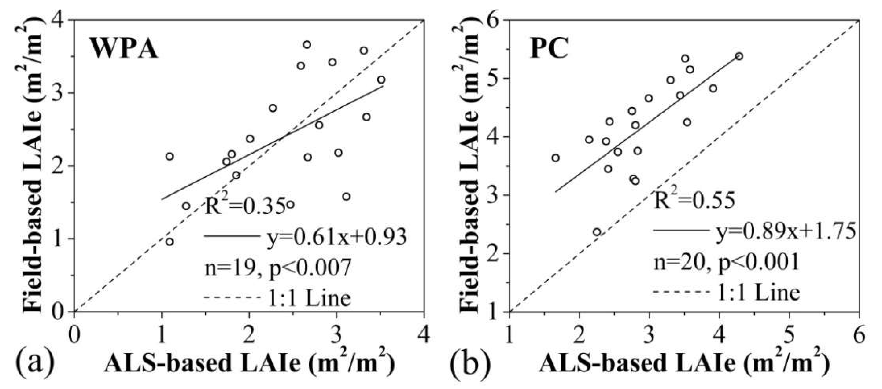
3.3.2. ALS-Based LAIe

The R² values of the statistical regression models between the ALS-based and field-based LAIe values were 0.35 and 0.55 in the WPA and PC sites, respectively (Figure 8). In addition, most ALS-based LAIe values were lower than the corresponding field-based LAIe values in the PC site (Figure 8b). We obtained ALS-based LAIe maps of WPA and PC (Figure 7c,g) and verified them (Table 4). In the WPA site, the RMSE of the ALS-based LAIe map was lower than the RMSE of the optical-based LAIe map. However, the RMSE of the ALS-based LAIe map was higher than the RMSE of the optical-based LAIe map in the PC site. We also found that most ALS-based LAIe values were lower than the field-based LAIe values in the verification plots for the PC site. The canopy cover and tree height of the PC site were generally higher than those of the WPA site (Table 1), while the sampling interval of the ALS data of PC was lower than those of WPA. Because of the occlusion effect of tall tree crowns and the limited penetration of laser beams, the description of the forest structure by point cloud will be incomplete, especially the structural information of the basal canopy. This may be the main reason for the underestimation of the ALS-based LAIe of the PC sites.

3.3.3. Stratified Forest Overstory LAIe

Based on the stratified overstory spectral imageries, we built NDVI-LAIe and SR-LAIe in both the WPA (Figure 6b,d) and PC (Figure 6f,h) sites. For comparison, we summarized the R² values of all the statistical regression models derived from the optical imageries, ALS data, and stratified overstory imageries and performed a leave-one-out cross-validation method [55] to evaluate the quality of these regression models (

Table 5. R² values and root mean square error of prediction (RMSEP) values of the statistical regression models from the optical imageries, stratified forest overstory imageries, and ALS data in both the WPA and PC sites.

Study Area	Data Type	Regression Model	R2	RMSEP
WPA	Optical imagery	NDVI-LAIe	0.17	0.79
		SR-LAIe	0.26	0.73
	Stratified forest	NDVI-LAIe	0.50	0.59
	overstory imagery	SR-LAIe	0.40	0.63
	ALS data		0.35	0.64
PC	Optical imagery	NDVI-LAIe	0.36	0.88
		SR-LAIe	0.51	0.58
	Stratified forest	NDVI-LAIe	0.62	0.51
	overstory imagery	SR-LAIe	0.53	0.56
	ALS data		0.55	0.57

). RMSEP is the root mean square error of prediction. Compared with the R² values of NDVI-LAIe from optical imageries, the R² values of NDVI-LAIe from the stratified overstory imageries increased by 0.33 and 0.26 in the WPA and PC sites, respectively. The improvements of SR-LAIe were smaller than those of NDVI-LAIe. The R² values of SR-LAIe increased by 0.14 and 0.02 in the WPA and PC sites, respectively. The R² values from the ALS data were higher than the R² values from the optical imageries and lower than the R² values of the NDVI-LAIe from stratified overstory imageries. Combining the quality evaluation results of the regression models, we found that the models from the stratified overstory imageries were the best, the models from the ALS data were the second, and the models from the optical imageries were the worst in both the WPA and PC sites. Moreover, in both the WPA and PC sites, NDVI was more accurate than SR for building regression models in stratified overstory imageries. This is the reason why we used NDVI-LAIe for mapping the LAIe.

We obtained the stratified forest overstory LAIe maps with a spatial resolution of 10 m in the WPA (Figure 7d) and PC (Figure 7h) sites. By verifying the LAIe maps (Table 4), we found that the RMSEs of the stratified overstory LAIe maps were the lowest among the three types of LAIe products in both the WPA and PC sites. Removing the forest background could overcome the underestimation of high LAIe values using the optical-based method effectively in a forest canopy.

4. Discussions

4.1. Tree Segmentation Accuracy Analysis

The parameters (i.e., DT and SSR) of tree crown segmentation algorithms are the key factors affecting the tree segmentation accuracy.The higher parameters can result in under-segmentations, whereas smaller parameters can result in over-segmentation [53]. We obtained the segmentation results of the study area by tuning the parameters using the forest plots. However, for the forest plots with different densities and different forest types in the study area, it is impossible to find the generic optimal segmentation parameters. Therefore, an improved method based on Li’s crown segmentation algorithm [56] may improve the segmentation results in landscape or region scales.

Forest density and type also affect the accuracy of tree crown segmentation. The segmentation results of medium- or low-density forest stands are better than those of high-density forest stands of the same forest type (Table 2). High-density forest stands have substantial overlapping between tree crowns, which increases the difficulty of identifying individual tree crown boundaries. Moreover, understory trees are not easy to be detected from high-density forest stands [53]. The segmentation accuracy of mixed forest stands is lower than single type forest stands with the same density (Table 2). The shape and size of the tree crowns vary significantly in the forest with abundant vegetation types, which increases the difficulty of tree segmentation. The crown segmentation algorithm in this paper has a strong ability to segment coniferous trees, while over-segmentation is easy to occur when some trees with long branches and broad-leaved trees with large crowns are segmented [57]. Recently, some advanced algorithms [58,59] for detecting different tree types and understory trees can be used in tree crown segmentation to improve the segmentation accuracy further.

In addition, the completeness of the forest point cloud is an essential factor affecting the segmentation accuracy. For example, tall trees might prevent the penetration of laser beams, which makes some point cloud of understory vegetation incomplete. This problem can be improved by increasing the laser pulse density or by using ALS data from multiple overlapping flight paths [54].

4.2. Effects of Removing Forest Background

T_num is a crucial factor affecting the accuracy of removing the forest background from an optical image. To study the effect of T_num, we generated stratified overstory imageries of the WPA and PC sites without using T_num (i.e., T_num = 0). Then, we calculated the proportions (P(0)) of the overstory pixel numbers to the total pixel numbers of the six test forest plots (i.e., WPA-LC, WPA-MC, WPA-HC, WPA-MM, PC-MC, and PC-HC) from these imageries. By comparing P(0) and the canopy cover (Table 3), we found that the differences (D(0)) between the P(0) and the canopy cover were 15%–29% in the forest plots of WPA, and the D(0) values were both 4 % in the forest plots of PC. It indicates that ignoring T_num will overestimate the number of forest overstory pixels in the stratified overstory imageries. When the overstory point cloud is transformed into a binary image based on the number of points, some grids with few overstory points tend to have a high proportion of the forest background. Without the T_num, these grids will be classified as overstory pixels, resulting in a high proportion of forest overstory in stratified overstory imageries.

The registration accuracy between the aerial imageries and ALS data also affects the accuracy of removing the forest background. To evaluate the registration accuracy of the WPA and PC sites, we respectively selected the landmarks (such as road intersection, house edge) using a visual method from the ALS-based intensity imageries and aerial imageries. We calculated the deviation in the 2-D horizontal direction (i.e., 2-D distance) of the aerial image coordinates and intensity image coordinates in each landmark (

Table 6. Registration error between the aerial imageries and ALS data in both the WPA and PC sites.

WPA Site				PC Site
Point	Δx(m)	Δy(m)	2-D Distance (m)	Point	Δx(m)	Δy(m)	2-D Distance (m)
1	4.95	1.88	5.29	1	−6.35	0.48	6.37
2	−0.95	0.74	1.21	2	0.4	1.85	1.9
3	1.98	−1.32	2.38	3	0.21	0.53	0.57
4	−0.4	−0.79	0.89	4	0.53	−3.44	3.48
5	1.91	1.48	2.41	5	−3.31	3.31	4.68
6	5.64	0.13	5.64	6	5.08	−1.06	5.19
7	6.08	1.06	6.18	7	−0.16	1.11	1.12
8	1.19	0.05	1.19	8	−2.86	2.43	3.75
9	2.64	−6.28	6.82	9	8.47	−0.79	8.5
10	0.99	−1.65	1.93	10	3.97	−1.59	4.27
11	3.18	−3.7	4.88	11	1.98	1.19	2.31
12	−0.64	−1.43	1.56	12	0.79	0.4	0.89
13	4.23	−0.63	4.28	13	4.63	0.33	4.64
14	3.7	0.79	3.79	14	1.43	−2.06	2.51
15	0.53	−0.21	0.57	15	2.25	0.53	2.31
Mean			3.27	16	−0.95	1.75	1.99
				17	1.48	0.95	1.76
				18	4.5	0.08	4.5
				19	1.45	−1.06	1.8
				20	0.12	0.79	0.8
				21	−2.86	3.33	4.39
				Mean			3.23

) as in Equation (2):

$$2-Ddistance=\sqrt{\Delta x^2+\Delta y^2},$$

(2)

where Δx and Δy represent the deviations of the aerial image and ALS data in the x-axis and y-axis direction, respectively. It was shown that the average deviations of landmarks were 3.27 and 3.23 m in the WPA and PC sites. For the WPA aerial imagery with a spatial resolution of 2.9 m, the registration error between the aerial imageries and ALS data is about one pixel. The registration error is about six pixels in the PC aerial imagery with a spatial resolution of 0.5 m.

4.3. Effects of VI-LAIe

Removing the forest background of optical imageries can effectively improve the VI-LAIe, and the degree of improvement is closely related to the canopy cover. To study the effects of the canopy cover on the VI-LAIe, we obtained the canopy cover of the forest plots for building VI-LAIe models (i.e., forest plot WPA-1~WPA-19 and PC-1~PC-20) by calculating the proportion of the overstory area to the total area of the plot (Table 1). According to the canopy cover, we divided these forest plots into three groups (i.e., the canopy cover ranges were 0.4–0.64, 0.65–0.84, and 0.85–1) to establish the NDVI-LAIe using toptical imageriehe s and stratified forest overstory imageries, respectively. By comparing the R² changes after removing the forest background (

Table 7. Comparison of R² values of the NDVI-LAIe using the optical imageries and stratified forest overstory imageries in different canopy cover ranges.

Study Area	Canopy Cover Range	Plot	Optical Imagery	Stratified Forest Overstory Imagery	Improvement
WPA	0.4–0.64	9	0.01	0.47	0.46
	0.65–0.84	9	0.48	0.71	0.23
	0.85–1	1	-	-	-
PC	0.4–0.64	0	−	−	−
	0.65–0.84	7	0.37	0.46	0.09
	0.85–1	13	0.73	0.73	0

), we found that the improvement of VI-LAIe decreased with the increase in canopy cover. The R² of the NDVI-LAIe increased by 0.46 and 0.23 using forest plots with a canopy cover of 0.4–0.64 and 0.65–0.84 in the WPA site. In the PC site, the R² of the NDVI-LAIe increased by 0.9 using forest plots with a canopy cover of 0.65–0.84, while the R² of the NDVI-LAIe did not improve using forest plots with a canopy cover of 0.85–1. In a forest stand with a low canopy cover, forest background accounts for a large proportion. However, the optical remotely sensed data could not adequately distinguish the mixed signals of the forest overstory and background, which introduces obvious errors in building the VI-LAIe. Therefore, the VI-LAIe improved significantly by removing the forest background. In a forest stand with a high canopy cover, because of the occlusion effect of tree crowns the optical remotely sensed data obtains less forest background information, and the point cloud of understory vegetation is difficult to remove. Thus, the removal of forest background had less impact on the VI-LAIe.

After removing the forest background, the degrees of improvement of VI-LAIe were different in the WPA and PC study areas. In addition to the 3-D forest structure, tree species, topography, and other factors, the use of different hyperspectral sensors is an important factor for this difference. In the HyMap data, we selected two bands with a central wavelength of 678 and 822 nm and a bandwidth of 15–16 nm to calculate the VIs. In the CASI data, we selected two bands with a central wavelength of 651 and 785 nm and a bandwidth of 3.6 nm to calculate the VIs. As shown in Figure 6, we found that the difference between the NDVI range of the WPA plots (i.e., 0.75–0.95) and the NDVI range of the PC plots (i.e., 0.55–0.85) was small. Meanwhile, the difference between the SR range of the WPA plots (i.e., 5–35) and the SR range of the PC plots (i.e., 5–8.5) was large. Because of the difference in the center wavelengths and bandwidths, the VI of the same type is different, which finally leads to the difference in the VI-LAIe. In the future, we can use the same spectral sensor to obtain optical imageries in different regions, which is conducive to a joint and comparative analysis of different regions.

4.4. Potential and Limitations of LAIe Mapping

In this article, the synthetic utilization of aerial spectral and laser scanning data could effectively improve the accuracy of mapping the forest canopy LAIe at the landscape or regional level, which can provide more reliable reference data for the validation of a coarse-resolution LAIe map or global LAI products. The unique feature of this study is to use the forest vertical stratification information from Lidar data to map the forest canopy LAIe. In the monitoring of multi-temporal LAI change, our method can be used to remove the disturbance of forest background to obtain the LAI change of the forest canopy. Moreover, the forest stratified method of Lidar not only contributes to the inversion of the overstory layer parameters, but also is conducive to obtaining the parameters of understory vegetation structure, which has the potential to be applied to forest management, carbon cycle, and ecological research [60,61,62]. At present, some studies have used the understory vegetation parameters derived from Lidar in fire behavior models, forest inventory, and wildlife habitat suitability [63,64,65].

It must be noted that there are some limitations to this study. In terms of data, our method needs Lidar data and optical imageries at the same time, which limits its application in wider areas. In the future, with the improvement of the global ALS database, point clouds in different regions will be connected with large-scale satellite images, which is conducive to the promotion of this method to larger regions. In terms of methods, we only used a linear regression model to estimate the canopy LAI; more models [2], such as polynomial, exponential, and logarithmic, should be considered and compared. In the selection of VI, we compared the effects of the forest background on the two types of VI (i.e., NDVI and SR), without making full use of the spectral information. In further research, we need to compare more VIs, especially the VIs that can mitigate background effects, to determine whether removing the forest background can improve most VIs. At present, some hyperspectral data and hyperspectral indices have been widely used in LAI estimation [66,67]. Therefore, we can also study the effect of removing the forest background on the hyperspectral indices. Moreover, our method has been tested in local areas, but it still needs to be verified in different forest types. Currently, there are many open-source point cloud data such as GlobALS [68] supporting this kind of verification, which means our method has the potential to be promoted in global products.

5. Conclusions

In this study, we developed a method of improving the estimation accuracy of forest overstory LAIe by combining aerial spectral imagery and ALS data. In addition, we compared and evaluated the accuracy of forest overstory LAIe maps from different combinations of optical and ALS data. Based on the results, we concluded that: (1) Removing forest background can effectively improve the estimation accuracy of optical-based forest LAIe. The improvement of NDVI-LAIe is more prominent; the R² increased by 0.33 and 0.26 in the WPA and PC sites, respectively. (2) The effect of forest background on forest stands with a low canopy cover is more evident than it is with forest stands with a high canopy cover. (3) The combination of ALS and optical remotely sensed data could obtain the best LAIe retrieval result effectively by removing the forest background information.

References

1. Chen, J.M.; Black, T.A. Defining leaf area index for non-flat leaves. Plant Cell Environ. 1992, 15, 421–429. [Google Scholar] [CrossRef]
2. Fang, H.; Baret, F.; Plummer, S.; Schaepman-Strub, G. An Overview of Global Leaf Area Index (LAI): Methods, Products, Validation, and Applications. Rev. Geophys. 2019, 57, 739–799. [Google Scholar] [CrossRef]
3. Asner, G.P.; Scurlock, J.M.O.; Hicke, J.A. Global synthesis of leaf area index observations: Implications for ecological and remote sensing studies. Glob. Ecol. Biogeogr. 2003, 12, 191–205. [Google Scholar] [CrossRef] [Green Version]
4. Meziane, D.; Shipley, B. Direct and Indirect Relationships between Specific Leaf Area, Leaf Nitrogen and Leaf Gas Exchange: Effects of Irradiance and Nutrient Supply. Ann. Bot. 2001, 88, 915–927. [Google Scholar] [CrossRef] [Green Version]
5. Law, B.E.; Falge, E.; Gu, L.; Baldocchi, D.D.; Bakwin, P.; Berbigier, P.; Davis, K.; Dolman, A.J.; Falk, M.; Fuentes, J.D. Environmental controls over carbon dioxide and water vapor exchange of terrestrial vegetation. Agric. Meteorol. 2002, 113, 97–120. [Google Scholar] [CrossRef] [Green Version]
6. Lindroth, A.; Lagergren, F.; Aurela, M.; Bjarnadottir, B.; Christensen, T.; Dellwik, E.; Grelle, A.; Ibrom, A.; Johansson, T.; Lankreijer, H. Leaf area index is the principal scaling parameter for both gross photosynthesis and ecosystem respiration of Northern deciduous and coniferous forests. Tellus B Chem. Phys. Meteorol. 2010, 60, 129–142. [Google Scholar] [CrossRef]
7. Baret, F.; Vanderbilt, V.C.; Steven, M.D.; Jacquemoud, S. Use of spectral analogy to evaluate canopy reflectance sensitivity to leaf optical properties. Remote Sens. Environ. 1994, 48, 253–260. [Google Scholar] [CrossRef]
8. Gray, J.; Song, C.H. Mapping leaf area index using spatial, spectral, and temporal information from multiple sensors. Remote Sens. Environ. 2012, 119, 173–183. [Google Scholar] [CrossRef]
9. Chen, J.M.; Black, T.A. Foliage area and architecture of plant canopies from sunfleck size distributions. Agric. Meteorol. 1992, 60, 249–266. [Google Scholar] [CrossRef]
10. Chen, J.M.; Rich, P.M.; Gower, S.T.; Norman, J.M.; Plummer, S. Leaf area index of boreal forests: Theory, techniques, and measurements. J. Geophys. Res. Atmos. 1997, 102, 29429–29443. [Google Scholar] [CrossRef]
11. Leblanc, S.G.; Chen, J.M.; Fernandes, R.; Deering, D.W.; Conley, A. Methodology comparison for canopy structure parameters extraction from digital hemispherical photography in boreal forests. Agric. Meteorol. 2005, 129, 187–207. [Google Scholar] [CrossRef] [Green Version]
12. Chopping, M.; Su, L.H.; Laliberte, A.; Rango, A.; Peters, D.P.C.; Kollikkathara, N. Mapping shrub abundance in desert grasslands using geometric-optical modeling and multi-angle remote sensing with CHRIS/Proba. Remote Sens. Environ. 2006, 104, 62–73. [Google Scholar] [CrossRef]
13. Pisek, J.; Chen, J.M. Mapping forest background reflectivity over North America with Multi-angle Imaging SpectroRadiometer (MISR) data. Remote Sens. Environ. 2009, 113, 2412–2423. [Google Scholar] [CrossRef]
14. Garrigues, S.; Lacaze, R.; Baret, F.; Morisette, J.T.; Weiss, M.; Nickeson, J.E.; Fernandes, R.; Plummer, S.; Shabanov, N.V.; Myneni, R.B.; et al. Validation and intercomparison of global Leaf Area Index products derived from remote sensing data. J. Geophys. Res. Biogeosci. 2008, 113, 20. [Google Scholar] [CrossRef]
15. Eriksson, H.M.; Eklundh, L.; Kuusk, A.; Nilson, T. Impact of understory vegetation on forest canopy reflectance and remotely sensed LAI estimates. Remote Sens. Environ. 2006, 103, 408–418. [Google Scholar] [CrossRef]
16. Wang, Y.J.; Woodcock, C.E.; Buermann, W.; Stenberg, P.; Voipio, P.; Smolander, H.; Hame, T.; Tian, Y.H.; Hu, J.N.; Knyazikhin, Y.; et al. Evaluation of the MODIS LAI algorithm at a coniferous forest site in Finland. Remote Sens. Environ. 2004, 91, 114–127. [Google Scholar] [CrossRef]
17. Abuelgasim, A.A.; Fernandes, R.A.; Leblanc, S.G. Evaluation of national and global LAI products derived from optical remote sensing instruments over Canada. IEEE Trans. Geosci. Electron. 2006, 44, 1872–1884. [Google Scholar] [CrossRef]
18. Ganguly, S.; Nemani, R.R.; Zhang, G.; Hashimoto, H.; Milesi, C.; Michaelis, A.; Wang, W.; Votava, P.; Samanta, A.; Melton, F. Generating global Leaf Area Index from Landsat: Algorithm formulation and demonstration. Remote Sens. Environ. 2012, 122, 185–202. [Google Scholar] [CrossRef] [Green Version]
19. Nemani, R.; Pierce, L.; Running, S.; Band, L. Forest ecosystem processes at the watershed scale: Sensitivity to remotely-sensed Leaf Area Index estimates. Int. J. Remote Sens. 1993, 14, 2519–2534. [Google Scholar] [CrossRef]
20. Huete, A.R. A soil-adjusted vegetation index (SAVI). Remote Sens. Environ. 1988, 25, 295–309. [Google Scholar] [CrossRef]
21. Brown, L.; Chen, J.M.; Leblanc, S.G.; Cihlar, J. A Shortwave Infrared Modification to the Simple Ratio for LAI Retrieval in Boreal Forests: An Image and Model Analysis. Remote Sens. Environ. 2000, 71, 16–25. [Google Scholar] [CrossRef]
22. Spanner, M.; Pierce, L.; Peterson, D.; Running, S. Remote sensing of temperate coniferous forest leaf area index The influence of canopy closure, understory vegetation and background reflectance. Int. J. Remote Sens. 1990, 11, 95–111. [Google Scholar] [CrossRef]
23. Baret, F.; Guyot, G. Potentials and limits of vegetation indices for LAI and APAR assessment. Remote Sens. Environ. 1991, 35, 161–173. [Google Scholar] [CrossRef]
24. Rautiainen, M. Retrieval of leaf area index for a coniferous forest by inverting a forest reflectance model. Remote Sens. Environ. 2005, 99, 295–303. [Google Scholar] [CrossRef]
25. Caetano, M.; Pereira, J.M. Effect of the understory on the estimation of coniferous forest leaf area index (LAI) based on remotely sensed data. Proc. Spie 1996, 2955, 63–71. [Google Scholar] [CrossRef]
26. Pisek, J.; Rautiainen, M.; Heiskanen, J.; Mõttus, M. Retrieval of seasonal dynamics of forest understory reflectance in a Northern European boreal forest from MODIS BRDF data. Remote Sens. Environ. 2012, 117, 464–468. [Google Scholar] [CrossRef]
27. Jiao, T.; Liu, R.; Liu, Y.; Pisek, J.; Chen, J.M. Mapping global seasonal forest background reflectivity with Multi-angle Imaging Spectroradiometer data. J. Geophys. Res. Biogeosci. 2014, 119, 1063–1077. [Google Scholar] [CrossRef]
28. Yang, L.; Liu, R.; Pisek, J.; Chen, J.M. Separating overstory and understory leaf area indices for global needleleaf and deciduous broadleaf forests by fusion of MODIS and MISR data. Biogeosciences 2017, 14, 1–32. [Google Scholar] [CrossRef] [Green Version]
29. Neyman, J. On a New Class of “Contagious” Distributions, Applicable in Entomology and Bacteriology. Ann. Math. Stat. 1939, 10, 35–57. [Google Scholar] [CrossRef]
30. Chen, J.M.; Leblanc, S.G. A four-scale bidirectional reflectance model based on canopy architecture. IEEE Trans. Geosci. Electron. 1997, 35, 1316–1337. [Google Scholar] [CrossRef]
31. Peduzzi, A.; Wynne, R.H.; Fox, T.R.; Nelson, R.F.; Thomas, V.A. Estimating leaf area index in intensively managed pine plantations using airborne laser scanner data. For. Ecol. Manag. 2012, 270, 54–65. [Google Scholar] [CrossRef] [Green Version]
32. Nilsson, M. Estimation of tree heights and stand volume using an airborne lidar system. Remote Sens. Environ. 1996, 56, 1–7. [Google Scholar] [CrossRef]
33. Lefsky, M.A.; Hudak, A.T.; Cohen, W.B.; Acker, S.A. Geographic variability in lidar predictions of forest stand structure in the Pacific Northwest. Remote Sens. Environ. 2005, 95, 532–548. [Google Scholar] [CrossRef] [Green Version]
34. Yan, G.; Hu, R.; Luo, J.; Marie, W.; Jiang, H.; Mu, X.; Xie, D.; Zhang, W. Review of indirect optical measurements of leaf area index: Recent advances, challenges, and perspectives. Agric. Meteorol. 2019, 265, 390–411. [Google Scholar] [CrossRef]
35. Lim, K.; Treitz, P.; Baldwin, K.; Morrison, I.; Green, J. Lidar remote sensing of biophysical properties of tolerant northern hardwood forests. Can. J. Remote Sens. 2003, 29, 658–678. [Google Scholar] [CrossRef]
36. Riaño, D.; Valladares, F.; Condés, S.; Chuvieco, E. Estimation of leaf area index and covered ground from airborne laser scanner (Lidar) in two contrasting forests. Agric. Meteorol. 2004, 124, 269–275. [Google Scholar] [CrossRef]
37. Roberts, S.D.; Dean, T.J.; Evans, D.L.; Mccombs, J.W.; Harrington, R.L.; Glass, P.A. Estimating individual tree leaf area in loblolly pine plantations using LiDAR-derived measurements of height and crown dimensions. For. Ecol. Manag. 2005, 213, 54–70. [Google Scholar] [CrossRef]
38. Richardson, J.J.; Moskal, L.M.; Kim, S.H. Modeling approaches to estimate effective leaf area index from aerial discrete-return LIDAR. Agric. Meteorol. 2009, 149, 1152–1160. [Google Scholar] [CrossRef]
39. Zhao, K.; Popescu, S. Lidar-based mapping of leaf area index and its use for validating GLOBCARBON satellite LAI product in a temperate forest of the southern USA. Remote Sens. Environ. 2009, 113, 1628–1645. [Google Scholar] [CrossRef]
40. Alonzo, M.; Bookhagen, B.; Mcfadden, J.P.; Sun, A.; Roberts, D.A. Mapping urban forest leaf area index with airborne lidar using penetration metrics and allometry. Remote Sens. Environ. 2015, 162, 141–153. [Google Scholar] [CrossRef]
41. Heiskanen, J.; Korhonen, L.; Hietanen, J.; Pellikka, P.K.E. Use of airborne lidar for estimating canopy gap fraction and leaf area index of tropical montane forests. Int. J. Remote Sens. 2015, 36, 2569–2583. [Google Scholar] [CrossRef]
42. Luo, S.; Wang, C.; Pan, F.; Xi, X.; Li, G.; Nie, S.; Xia, S. Estimation of wetland vegetation height and leaf area index using airborne laser scanning data. Ecol. Indic. 2015, 48, 550–559. [Google Scholar] [CrossRef]
43. Koch, B. Status and future of laser scanning, synthetic aperture radar and hyperspectral remote sensing data for forest biomass assessment. J. Photogramm. Remote Sens. 2010, 65, 581–590. [Google Scholar] [CrossRef]
44. Clark, M.L.; Roberts, D.A.; Ewel, J.J.; Clark, D.B. Estimation of tropical rain forest aboveground biomass with small-footprint lidar and hyperspectral sensors. Remote Sens. Environ. 2011, 115, 2931–2942. [Google Scholar] [CrossRef]
45. Tonolli, S.; Dalponte, M.; Neteler, M.; Rodeghiero, M.; Vescovo, L.; Gianelle, D. Fusion of airborne LiDAR and satellite multispectral data for the estimation of timber volume in the Southern Alps. Remote Sens. Environ. 2011, 115, 2486–2498. [Google Scholar] [CrossRef]
46. Shang, C.; Treitz, P.; Caspersen, J.; Jones, T. Estimation of forest structural and compositional variables using ALS data and multi-seasonal satellite imagery. Int. J. Appl. Earth Obs. Geoinf. 2019, 78, 360–371. [Google Scholar] [CrossRef]
47. Frazer, R.B.G.W.; Canham, C.D.; Lertzman, K.P. Gap Light Analyzer, Version 2.0. Available online: http://www.rem.sfu.ca/forestry/index.htm (accessed on 23 February 2019).
48. Zheng, G.; Moskal, L.M.; Kim, S.-H. Retrieval of Effective Leaf Area Index in Heterogeneous Forests with Terrestrial Laser Scanning. IEEE Trans. Geosci. Electron. 2013, 51, 777–786. [Google Scholar] [CrossRef]
49. Lu, L.; Zheng, G.; Ma, L. Combining point cloud slicing and terrestrial laser scanning data to retrieve an effective leaf area index. J. Remote Sens. 2018, 22, 432–449. [Google Scholar] [CrossRef]
50. Zhang, W.; Qi, J.; Wan, P.; Wang, H.; Xie, D.; Wang, X.; Yan, G. An Easy-to-Use Airborne LiDAR Data Filtering Method Based on Cloth Simulation. Remote Sens. 2016, 8, 501. [Google Scholar] [CrossRef]
51. CloudCompare. Available online: http://www.cloudcompare.org/ (accessed on 20 July 2019).
52. McGaughey, R.J. FUSION: LIDAR & IFSAR Tools. Available online: http://forsys.cfr.washington.edu/JFSP06/lidar_&_ifsar_tools.htm (accessed on 9 August 2019).
53. Li, W.; Guo, Q.; Jakubowski, M.K.; Kelly, M. A New Method for Segmenting Individual Trees from the Lidar Point Cloud. Photogramm. Eng. Remote Sens. 2012, 78, 75–84. [Google Scholar] [CrossRef] [Green Version]
54. Zheng, G.; Ma, L.; Eitel, J.U.H.; Wei, H.; Li, M. Retrieving Directional Gap Fraction, Extinction Coefficient, and Effective Leaf Area Index by Incorporating Scan Angle Information From Discrete Aerial Lidar Data. IEEE Trans. Geosci. Remote Sens. 2016, 55, 577–590. [Google Scholar] [CrossRef]
55. Geisser, S. A Predictive Approach to the Random Effect Model. Biometrika 1974, 61. [Google Scholar] [CrossRef]
56. Wang, X.; Zheng, G.; Yun, Z.; Moskal, L. Characterizing Tree Spatial Distribution Patterns Using Discrete Aerial Lidar Data. Remote Sens. 2020, 12, 712. [Google Scholar] [CrossRef] [Green Version]
57. Wallace, L.; Lucieer, A.; Watson, C.S. Evaluating Tree Detection and Segmentation Routines on Very High Resolution UAV LiDAR Data. IEEE Trans. Geosci. Electron. 2014, 52, 7619–7628. [Google Scholar] [CrossRef]
58. Hamraz, H.; Contreras, M.A.; Zhang, J. A robust approach for tree segmentation in deciduous forests using small-footprint airborne LiDAR data. Int. J. Appl. Earth Obs. Geoinf. 2016, 52, 532–541. [Google Scholar] [CrossRef] [Green Version]
59. Paris, C.; Valduga, D.; Bruzzone, L. A Hierarchical Approach to Three-Dimensional Segmentation of LiDAR Data at Single-Tree Level in a Multilayered Forest. IEEE Trans. Geosci. Electron. 2016, 54, 1–14. [Google Scholar] [CrossRef]
60. Ares, A.; Neill, A.R.; Puettmann, K.J. Understory abundance, species diversity and functional attribute response to thinning in coniferous stands. For. Ecol. Manag. 2010, 260, 1104–1113. [Google Scholar] [CrossRef]
61. Van Miegroet, H.; Nicholas, N.S.; Moore, P. Relative role of understory and overstory in carbon and nitrogen cycling in a southern Appalachian spruce-fir forest. Can. J. For. Res. 2007, 115, 231–242. [Google Scholar] [CrossRef]
62. Camprodon, J.; Brotons, L. Effects of undergrowth clearing on the bird communities of the Northwestern Mediterranean Coppice Holm oak forests. For. Ecol. Manag. 2006, 221, 72–82. [Google Scholar] [CrossRef]
63. Riano, D.; Meier, E.; Allgower, B.; Chuvieco, E.; Ustin, S.L. Modeling airborne laser scanning data for the spatial generation of critical forest parameters in fire behavior modeling. Remote Sens. Environ. 2003, 86, 177–186. [Google Scholar] [CrossRef]
64. Bouvier, M.; Durrieu, S.; Fournier, R.A.; Renaud, J.P. Generalizing predictive models of forest inventory attributes using an area-based approach with airborne LiDAR data. Remote Sens. Environ. 2015, 156, 322–334. [Google Scholar] [CrossRef]
65. Martinuzzi, S.; Vierling, L.A.; Gould, W.A.; Falkowski, M.J.; Evans, J.S.; Hudak, A.T.; Vierling, K.T. Mapping snags and understory shrubs for a LiDAR-based assessment of wildlife habitat suitability. Remote Sens. Environ. 2009, 113, 2533–2546. [Google Scholar] [CrossRef] [Green Version]
66. Liang, L.; Di, L.; Zhang, L.; Deng, M.; Qin, Z.; Zhao, S.; Lin, H. Estimation of crop LAI using hyperspectral vegetation indices and a hybrid inversion method. Remote Sens. Environ. 2015, 165, 123–134. [Google Scholar] [CrossRef]
67. Lee, K.-S.; Cohen, W.B.; Kennedy, R.E.; Maiersperger, T.K.; Gower, S.T. Hyperspectral versus multispectral data for estimating leaf area index in four different biomes. Remote Sens. Environ. 2004, 91, 508–520. [Google Scholar] [CrossRef]
68. Stereńczak, K.; Vaglio Laurin, G.; Chirici, G.; Coomes, D.; Dalponte, M.; Latifi, H.; Puletti, N. Remote sensing Global Airborne Laser Scanning Data Providers Database (GlobALS)—A New Tool for Monitoring Ecosystems and Biodiversity. Remote Sens. 2020, 12, 1877. [Google Scholar] [CrossRef]
Figure 1. The study area. The subfigures (a,b) show the aerial false-color images and effective leaf area index (LAIe) measurement locations of the digital hemispherical photo (DHP) and terrestrial laser scanning (TLS) in the Washington Park Arboretum (WPA) and Panther Creek (PC) sites. The subfigures (d,c) show a DHP and the corresponding aerial laser scanning (ALS) data (circular forest plot with a radius of 30m) from the PC site. The subfigures (f,e) show a DHP and the corresponding ALS data (circular forest plot with a radius of 30m) from the WPA site. The subfigures (g,h) are the ALS data of the WPA and PC sites.
Remotesensing 12 02126 g001
Figure 2. Flowchart of improving the forest overstory LAIe estimation by combining the aerial spectral and laser scanning data.
Remotesensing 12 02126 g002
Figure 3. Determination of the height threshold for stratifying the forest overstory and background using the ALS data in the WPA (a) and PC (b) study sites.
Remotesensing 12 02126 g003
Figure 4. Height-normalized ALS data (insets a,c,e,g,i,k) and corresponding tree segmentation results (insets b,d,f,h,j,l) of six circular forest plots with a radius of 30 m, including the WPA-LC, WPA-MC, WPA-HC, WPA-MM, PC-MC, and PC-HC. In the tree segmentation results, different colors represent individual trees.
Remotesensing 12 02126 g004
Figure 5. Forest stratification results in both the WPA and PC sites. (a) Point cloud of overstory layer in the WPA site. (b) Point cloud of understory layer in the WPA site. (c) Binary image in the WPA site where the forest overstory and background are represented by green and red. (d) Point cloud of the overstory layer in the PC site. (e) Point cloud of the understory layer in the PC site. (f) Binary image in the PC site where the forest overstory and background are represented by green and red. Height-normalized ALS data (insets g,i,k,m) and corresponding stratification results (insets h,j,l,n) of four east-west line transects with a length of 60 m, including WPA-L1, WPA-L2, PC-L1, and PC-L2. In the stratification results of the line transects, the forest overstory and understory are represented by green and red.
Remotesensing 12 02126 g005
Figure 6. The linear regression statistical models of vegetation index and field-based LAIe in both the WPA and PC sites. (a) Normalized difference vegetation index (NDVI)-LAIe from the optical image in the WPA site. (b) NDVI-LAIe from the stratified forest overstory image in the WPA site. (c) SR-LAIe from the optical image in the WPA site. (d) Simple ratio (SR)-LAIe from the stratified forest overstory image in the WPA site. (e) NDVI-LAIe from the optical image in the PC site. (f) NDVI-LAIe from the stratified forest overstory image in the PC site. (g) SR-LAIe from the optical image in the PC site. (h) SR-LAIe from the stratified forest overstory image in the PC site.
Remotesensing 12 02126 g006
Figure 7. LAIe mapping results in both the WPA and PC sites. (a) The optical image in the true color of the WPA site. (b) Optical-based LAIe map of the WPA site. (c) ALS-based LAIe map of the WPA site. (d) Stratified forest overstory LAIe map of the WPA site. (e) The optical image in the true color of the PC site. (f) Optical-based LAIe map of the PC site. (g) ALS-based LAIe map of the PC site. (h) Stratified forest overstory LAIe map of the PC site.
Remotesensing 12 02126 g007
Figure 8. Comparison between the ALS-based LAIe values and the field-based LAIe values of forest plots in WPA (a) and PC (b) sites.
Remotesensing 12 02126 g008