Learning to Classify Structures in ALS-Derived Visualizations of Ancient Maya Settlements with CNN


1
Research Centre of the Slovenian Academy of Sciences and Arts (ZRC SAZU), Novi trg 2, 1000 Ljubljana, Slovenia
2
Information and Communication Technologies, Jožef Stefan International Postgraduate School, Jamova cesta 39, 1000 Ljubljana, Slovenia
3
Jožef Stefan Institute, Jamova cesta 39, 1000 Ljubljana, Slovenia
*
Author to whom correspondence should be addressed.
Remote Sens. 2020, 12(14), 2215; https://0-doi-org.brum.beds.ac.uk/10.3390/rs12142215
Submission received: 5 June 2020
/
Revised: 4 July 2020
/
Accepted: 4 July 2020
/
Published: 10 July 2020
(This article belongs to the Special Issue Remote Sensing of Archaeology)
Abstract
:Archaeologists engaging with Airborne Laser Scanning (ALS) data rely heavily on manual inspection of various derived visualizations. However, manual inspection of ALS data is extremely time-consuming and as such presents a major bottleneck in the data analysis workflow. We have therefore set out to learn and test a deep neural network model for classifying from previously manually annotated ancient Maya structures of the Chactún archaeological site in Campeche, Mexico. We considered several variations of the VGG-19 Convolutional Neural Network (CNN) to solve the task of classifying visualized example structures from previously manually annotated ALS images of man-made aguadas, buildings and platforms, as well as images of surrounding terrain (four classes and over 12,000 anthropogenic structures). We investigated how various parameters impact model performance, using: (a) six different visualization blends, (b) two different edge buffer sizes, (c) additional data augmentation and (d) architectures with different numbers of untrainable, frozen layers at the beginning of the network. Many of the models learned under the different scenarios exceeded the overall classification accuracy of 95%. Using overall accuracy, terrain precision and recall (detection rate) per class of anthropogenic structure as criteria, we selected visualization with slope, sky-view factor and positive openness in separate bands; image samples with a two-pixels edge buffer; Keras data augmentation; and five frozen layers as the optimal combination of building blocks for learning our CNN model.

1. Introduction
Archaeologists engaging with airborne laser scanning (ALS) data rely heavily on manual inspection. For this purpose, raw data is most often converted into some derivative of a digital elevation model that the interpreter regards useful for visual examination [1,2,3,4,5,6]. In our own study of ancient Maya settlements, manual analysis and annotation of visualized ALS data for an area of 130 km2 took about 8 man-months (the equivalent of a single person working full-time for 8 months) to complete.
Practice shows that manual inspection is extremely time-consuming [7,8] and as such presents a major bottleneck in the data analysis workflow. Continuing along this path without a more efficient solution, it is not only going to be impossible to keep up with ever-increasing data volumes but also very difficult to remove the inherent bias of the human observer [9]. This gives rise to a pressing need for computational methods that would automate data annotation and analysis and thus replace or at least considerably speed up manual work, saving time that can be used to do actual research. Although a machine learning algorithm can not completely eliminate the biases of people preparing and annotating the dataset that the computer learns from, such an algorithm can at least average out the biases of individual contributors, who are affected by their individual experiences, knowledge, observations and expectations [9].
Deep Convolutional Neural Networks (CNNs), the computational methods currently dominating the field of computer vision, are state-of-the-art tools-of-choice for tasks such as image classification and object detection [10,11,12,13]. While the majority of existing CNN models are trained on (and used with) realistic photographic images “of everyday life” as input [14,15,16,17], these models can be adapted to perform just as well on datasets with images highly specific to narrow domains [18,19,20,21,22,23] with use of transfer learning, and of different modalities [24,25,26,27]. Many such CNN models have been adapted for medical imaging, for instance, for classification of Magnetic Resonance Imaging (MRI) [28,29] and Computed Tomography (CT) scans [30], some of which surpass the classification capabilities of an expert in the field [31,32]. Pre-trained CNNs also allow us to use these techniques for tasks that do not have a large number of training samples available, as is often the case in archaeology. While there have been many applications of CNNs in remote sensing [22,25,33,34,35,36,37,38,39,40,41], only a few of these concern ALS data in archaeological prospection [42,43,44,45,46,47,48].
The main objective of this paper is to determine whether we can successfully classify the three most common types of ancient Maya structures against natural terrain by using a CNN model with an ALS visualization as an input. We set out to compare the performance of CNN models using six different ALS visualizations. Additionally, we wanted to know how to best prepare the image samples; specifically, we wanted to know if sample images of individual structures that include some of their immediate surroundings lead to CNNs that perform better as compared to CNNs that work with images where surroundings are excluded. We also examine how data augmentation improves the performance of the CNN model because the number of our samples is significantly lower (in the order of thousands) than the number of samples usually used for training CNN models (in the order of millions). Since we start with an initialized network with pre-trained weights, we were interested to find out how the number of neural network layers frozen during training impacts the final model performance.
The paper first describes our case study area, ALS data and processing procedures (Section 2.1). This is followed by description of the image annotation process (Section 2.2). We proceed with a description of the experimental setup, specifically with an explanation of how we generated the dataset for the classification task (Section 3.1), selected the CNN architecture (Section 3.2) and set up the experimental design (Section 3.3) for learning and testing CNN models. We present the model performance results for all scenarios in Section 4 and discuss these in Section 5; we analyze misclassifications (Section 5.1), compare results of different visualizations (Section 5.2), examine the influence of the buffer size (Section 5.3) and the number of frozen layers (Section 5.4), evaluate the effects of data augmentation (Section 5.5) and discuss the feasibility of the model to replace manual annotation work (Section 5.6). Our conclusions are summarized in Section 6.
2. Data and Methods
2.1. Study Area, Data and Data Processing
The research area covers 230 km2 around Chactún, one of the largest Maya urban centers known so far in the central lowlands of the Yucatan peninsula, located in the northern sector of the depopulated Calakmul Biosphere Reserve in Campeche, Mexico (Figure 1). The area is characterized by low hills, “bulging” a few tens of meters (typically not more than 30 m) above the surrounding seasonal wetlands (bajos). It is completely covered by tropical semi-deciduous forest (Figure 2). The overall elevation range is only from 220 m to 295 m (or 300 m when buildings are included).
Chatún’s urban core, composed of three concentrations of monumental architecture, was discovered in 2013 by prof. Šprajc and his team [49]. It has several plazas surrounded by temple-pyramids, massive palace-like buildings and two ball courts. A large rectangular water reservoir lies immediately to the west of the main groups of structures. Ceramics collected from the ground surface, the architectural characteristics and dated monuments indicate that the center started to thrive in the Preclassic period (c. 1000 BC–250 AD), reaching its climax during the Late Classic (c. 600–1000 AD) and had an important role in the regional political hierarchy [49,50]. To the south of Chactún are Lagunita and Tamchén, both prominent urban centers, as well as numerous smaller building clusters scattered on the hills of the research area [51,52].
Airborne laser scanning data around Chactún was collected at the end (peak) of the dry season in May 2016. Mission planning, data acquisition and data processing were carried out with clear archaeological purposes in mind. The National Centre for Airborne Laser Mapping (NCALM) was commissioned for data acquisition and initial data processing (conversion from full-waveform to point cloud data; ground classification) [53,54], while the final processing (additional ground classification; visualization) was performed by ZRC SAZU. The density of the final point cloud and the quality of the derived elevation model proved excellent for detection and interpretation of archaeological features (Table 1), with very few processing artifacts discovered.
Ground points were classified with the Terrascan software, and algorithm settings were optimized to remove only the vegetation cover and leave remains of past human activities as intact as possible (Table 2). Ground points therefore also include remains of buildings, walls, terracing, mounds, chultuns (cisterns), sacbeob (raised paved roads), and drainage channels. The average density of ground returns from a combined dataset comprising information from all flights and all three channels is 14.7 pts/m2—enough to provide a high-quality digital elevation model (DEM) with a 0.5 m spatial resolution. The rare areas with no ground returns include aguadas (artificial rainwater reservoirs) with water.
2.2. Data Annotations
We used visualization for archaeological topography (VAT) [6] and a locally stretched elevation model to annotate buildings and platforms, as well as local dominance [55] to annotate aguadas. Local dominance shows the slightly raised embankments on the outer edges of aguadas, which does not exist around natural-occurring depressions.
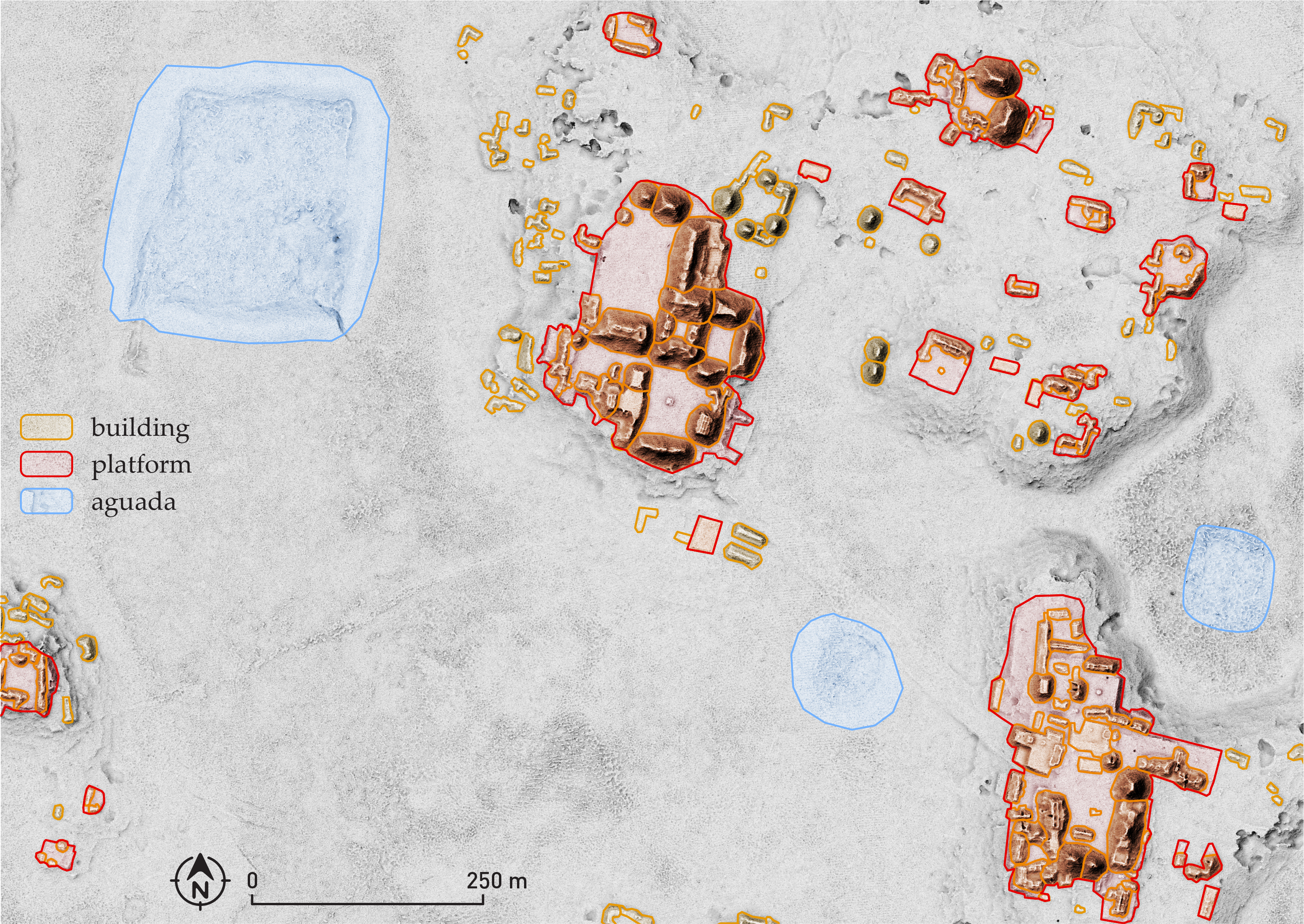
The exact boundaries were drawn on the outer edges of walls or collapsed material. Due to the configuration and state of structures, it was not always possible to delineate each construction—therefore, a single polygon may encompass several buildings (Figure 3). We annotated aguadas in the whole study area and buildings and platforms in its southern part (130 km2).
Figure 4 shows annotated buildings, which include pyramids (a), ball-courts (b), palace-like buildings (c), remnants of dwellings (d) and other architectural features supporting roofed areas (e).
Artificial terrain flattenings, elevated from the surrounding ground, were annotated as platforms (Figure 5). We only annotated platforms that were not used for agricultural purposes, i.e., we excluded agricultural terraces.
Aguadas are structures specific to and typical of ancient Maya lowland landscape. They are artificial modifications (deepening) of the terrain, usually with pronounced (slightly raised) edges. They functioned as water reservoirs—artificial ponds or lakes (Figure 6). For annotation of aguadas, we sometimes used additional visualization that accentuated embankments, for instance, local dominance or flat terrain VAT (Figure 7).
3. Experimental Setup
We developed a classification model, based on CNN, that distinguishes among four different classes: building, platform, aguada and terrain. To this end, we produced thousands of smaller image samples for each class, cut from the ALS visualizations over the study area. These generated samples, rather than the visualization of the whole area, were then used as inputs for learning and testing the CNN models. The scale is not uniform.
3.1. Generating the Dataset for the Classification
We determined a square bounding box with an additional edge buffer (2 and 15 pixels, respectively, for two dataset variants)—a patch—for every anthropogenic structure, and exported that part of the visualization as a sample for either a building, a platform or an aguada (Figure 4, Figure 5 and Figure 6, respectively). Along with the image samples of the three classes representing anthropogenic structures, we added terrain as a fourth class representing a “negative class” (the background). Terrain (Figure 8) was not annotated; therefore, square patches were randomly selected from the whole study area, making sure the patch contained no (part of) annotated structures. Terrain samples are all 128 by 128 pixels so that they are comparably sized to samples of structures and match the input size of our neural network. We generated enough terrain samples to match the combined count of building, platform and aguada samples. When generating terrain samples, we had to make sure that they did not intersect an annotated structure, and that the selected patch did not have any no-data pixels. The same was true for structure samples as well; patches at the edge of the study area that included no-data pixels were omitted when generating datasets. For this reason, the testing set for aguadas with a 15-pixels buffer contains four samples less (one aguada less) than the testing set with a 2-pixels buffer. The same is true for platforms and buildings; there are a few samples less in the 15-pixels buffer dataset.
In total, we produced 8706 samples of buildings, 2093 samples of platforms and 95 samples of aguadas. Because the total count of the latter was very low, we produced three additional image samples for each aguada by rotating the visualizations by 90°, 180° and 270°, generating 380 aguada samples in total. For visualizations where hillshading was used, we also adjusted the sun azimuth so that shading direction is preserved and consistent across all final image samples (Figure 9). The scale is uniform.
We divided the sample images of all four classes into training and testing sets, containing roughly 80% and 20% of the image samples, respectively (Table 3). The dataset was not split randomly, but according to the geographic location (Figure 2). There were two reasons for this: (1) Buildings were often built on top of platforms and platforms often contained multiple buildings. Therefore, the image samples of buildings and platforms overlap. We had to assure images with overlapping objects are all in the same dataset, either in the training or the testing set, but not split between them. (2) Because terrain samples were generated randomly, some parts of the terrain could be contained in multiple image samples. Again, the best solution is to split the generated image samples according to location, so no two images of the same area could be in both the training and the testing set. Despite the random selection of terrain patches, the same locations were used for testing of all visualizations.
3.2. CNN Architecture
We used the VGG network [56], a deep CNN architecture, for transfer learning. There are two variations of the network, the VGG-16 (13 convolutional layers and three fully connected layers) and the VGG-19 (16 convolutional layers and three fully connected layers), and both use very small (3 by 3) convolutional filters. There have been previous uses of the VGG network, where solutions (CNN architecture) either fully or partially rely on the VGG network, in other remote sensing studies [57,58,59,60,61].
Our CNN model, based on VGG-19, was implemented in Python with the Keras and TensorFlow libraries. Image samples were scaled to the input size of 128 by 128 pixels before they were fed into the network. We decided to use pre-trained weights and fine-tune the network, rather than fully train it, as similar remote sensing studies pointed out that this tends to be the best performing strategy [62]. We initialized the network with weights pre-trained on ImageNet [14] and froze the first few layers of the network so that their weights were not updated during backpropagation. We can freeze the pre-set weights for neurons of the top (first) few layers that recognize lines, edges and simple geometric shapes. These visual features are not domain-specific, and the weights set for these neurons have been thoroughly trained on millions of images. However, the weights of neurons at the bottom (end) layers of the network still need to be fine-tuned [63] for our specific task of classification of anthropogenic objects on ALS visualization; therefore, these layers remain trainable.
Our training dataset consists of roughly 17,000 images (rather than millions that would be required ideally). This is a rather small training set for image recognition tasks. With such cases, measures to prevent a model from overfitting the training set should be implemented [64]. For this purpose, a dropout layer was inserted towards the end part of the network. In the dropout layer, neurons and their connections are randomly dropped out (in our case 50% of them, which is a common practice). This regularization method prevents the network from memorization of training samples and instead encourages the network to learn more general representations. Generalization capabilities are thus improved—leading to better model performance on unseen data—resulting in the final model being more robust [65].
3.3. Experimental Design
We trained and tested the neural network in different scenarios, examining how different combinations of parameters and visualizations used affect the predictive capabilities of the resulting model.
To find the best visualization for the image classification task, we compared image inputs, generated from the following visualizations:
- Flat VAT; VAT with visualization parameters adjusted to show minute topographic variations in a level surface.
- VAT-HS; VAT without analytical hillshading (HS), as one grayscale composite (one channel).
- VAT-HS channels; slope, positive openness and sky-view factor—where layers are not combined, but fed into separate channels of the image/input layer.
- Red relief image map (RRIM); often used for manual interpretation, because it is direction-independent and easy to interpret. It overlays a slope gradient image, colored in white to red tones, with the “ridge and valley index” computed from positive and negative openness in a grayscale colormap [67,68].
- Local dominance (LD) is well suited for very subtle positive topographic features and depressions [2]. We included it to test its performance against flat VAT.
To determine the optimal preparation of image samples, we tested image samples with two sizes for the edge buffer around bounding boxes:
- 15-pixels to represent a loose edge that includes some immediate surrounding, and
- 2-pixels for a tight edge. We kept 1 m of surrounding terrain around structures, because of the positional uncertainty of hand-drawn polygons.
When we generated image samples, as described previously, we always replicated each aguada three more times with rotations. However, we also used either:
- no additional data augmentation, or
- Keras library data augmentation. Applied augmentations include zoom range, width shift range and height shift range. We did not use rotation and flip, because these would result in inconsistent relief shading and distorted orientation of buildings, which are often aligned to a certain direction.
Finally, we considered two variations of the VGG-19 architecture with different degrees of trainability. The two neural networks were initialized with either of the architectures:
- 3 frozen (untrainable) layers at the top or
- 5 frozen layers at the top.
We consider the above dimensions as independent. We tested all possible combinations of visualizations, edge buffer, data augmentation and number of frozen layers, which resulted in 48 different scenarios.
All of the layers of our network are represented in the architecture diagram (Figure 10). Layers at the top of the network are represented at the left side.
4. Results
For every scenario, the model performance was measured in terms of overall accuracy, precision for the terrain class and recall for the classes of anthropogenic structures (building, platform, aguada).
Accuracy (overall accuracy) gives us an initial evaluation of model performance in general, over all classes. While our classes have different numbers of training samples, no anthropogenic structure is more important than another (and neither is the terrain); we thus opted for non-weighted average accuracy.
Models with high overall accuracy—in our results many score above 0.95, as shown in Scheme 1—are good candidates for final model selection, even though the accuracy itself is not a sufficient measure to evaluate model performance.
Ideally, our final model would also:
- minimize false-negative results of anthropogenic structures’ classes since we do not want structures to go unrecognized. Minimizing these false negatives would result in high recall for building, platform and aguada classes. Recall (also known as detection rate or sensitivity) can be defined as the probability of detection; the proportion of the actual positive samples that have been correctly classified as such.
- minimize false-positive results for the terrain class, since we do not want any structure to be misclassified as terrain—it is, in fact, better for one type of structure to be misclassified as a different type of structure. Minimizing terrain false positives leads to high precision for the terrain class. Precision is the fraction of true positive samples among those that were classified as positive ones.
5. Discussion
The results presented in Scheme 1 show that many of the tested models can successfully classify the three types of anthropogenic structures against the natural terrain, with accuracies of 95% and above. When using a model with terrain precision of over 99.5% (rounded up to 1.0 in Scheme 1), only less than 0.5% of anthropogenic structures would be missed by not inspecting samples classified as terrain. It is also important to note that even archaeologists inspecting ALS visualizations are not always sure how to annotate a certain feature, as in many cases it is not as obvious whether a feature is natural or anthropogenic. However, when using models with terrain precision of 0.995 and above, only 0.5% of anthropogenic structures would be misclassified as terrain, the other errors would include an anthropogenic structure misclassified as belonging to another class of anthropogenic structures. From an archaeological point of view, it is better to confuse an anthropogenic structure with another type of anthropogenic structure, than to misinterpret it as terrain (e.g., for estimating the man-power needed for construction or for population estimates).
5.1. Analysis of Misclassifications
Here we analyze the misclassifications made by the learned model by the VAT-HS visualization for generating image samples with a 2-pixel edge buffer around each structure’s bounding box. This visualization is one of the two that achieved the highest performance and is the one that is visually most similar to VAT, which was used for the manual annotation in our study, as well as many others. The CNN model was learned with the top five frozen layers and with no additional data augmentation. The resulting model achieves 98% overall accuracy (Scheme 1).
It is evident from the confusion matrix (Figure 11) that the most common type of classification error is misclassifying platforms as buildings, which is also true for most of the other tested scenarios. Visual inspection reveals that the misclassified platform samples usually contain a single building on a platform (Figure 12a,b), a string of buildings and multiple buildings on a larger platform (Figure 12c) or a smaller platform with particularly pronounced edges that in itself resembles a building (Figure 12d).
Very low platforms are sometimes misclassified as terrain (Figure 13a) or as an aguada (Figure 13b). Vice versa, certain image samples with a mixture of steep and flat terrain (Figure 13c) and aguadas with steep banks (Figure 13d) are also misclassified as platforms.
Some aguadas can be rather easily mistaken for natural formations because many have very indistinct edges (Figure 6 and Figure 14a). The reverse is even more common; terrain is misclassified as an aguada in areas with a rougher surface, which we think is a highly porous limestone on the edge of a bajo (Figure 14b).
Inspection of false positives for the aguada, building and platform classes additionally reveals a number of terrain samples that contain unannotated anthropogenic structures (e.g., walls, stone piles, agricultural terraces, tracks, quarries, chultuns), which results in the misclassification of terrain samples (Figure 14c,d). Some other natural formations could resemble man-made structures as well, but these do not seem to appear frequently within our study area. They could be either smaller, steep or rugged formations, the size of a house or a palace, thus resembling ruins of a building; or natural flattening of a larger area that could be mistaken for a platform. This could present a potential issue for the algorithm, and sometimes even for the archaeologists doing manual annotation, if the ALS data itself are noisy or if the archaeological features are too heavily eroded to be easily distinguished. We believe the model works better when the terrain characteristics are quite different from the archaeological features. In any case, all terrain samples should ideally be checked for accuracy of annotations, but it is this time-consuming process we try to avoid with the use of our CNN models. Thus, the best-performing models are those that achieve not only high accuracy but also terrain precision close to 100%—meaning there are almost no anthropogenic structures misclassified as terrain. This saves time because double checking samples classified as terrain is unnecessary, and potentially only visual checking of samples classified as aguadas, buildings, or platforms is required. Therefore, we want primarily to have high accuracies for these three structures classes; yet as a consequence, this would also result in better model performance on the terrain class.
5.2. Comparison of Visualizations
Comparison of the performance of models for different visualizations reveals that no single visualization is categorically better than others. However, we notice that VAT-HS and VAT-HS channels (with accuracies of the best models reaching 98% and 99%, respectively) seem to have some advantage over VAT and Flat VAT in most of the test scenarios. Drawing conclusions from these results, the addition of hillshading into the visualization blend seems to be hindering the model performance. However, hillshading appears to remain a subjective preference for many of the researchers in archaeology and remote sensing that visually inspect ALS visualizations. This preference may only exist due to our human real-life experience and a more intuitive understanding of hillshading compared to other visualizations. Additionally, a person can better inspect a single visualization blend than three separate visualizations, while the same is not necessarily true for CNN classification models. The VAT-HS channels visualization that includes slope, positive openness and sky-view factor in separate channels in most cases performs better than VAT-HS, which blends the three into a single grayscale image. The preference for VAT-HS or VAT-HS channels does not present an issue in practice because either can achieve good results. What makes the difference is knowing—or finding—how to initialize the parameters of the neural network to optimize the performance of the final CNN classification model.
RRIM visualization performed well, achieving accuracy of up to 96%, while LD produced unsatisfactory results with accuracy ranging from 45% to 70%. Terrain precision with LD is often at 100%, meaning there are no false positives for terrain, but that is because almost all samples are classified as buildings. This could be connected to buildings and platforms appearing too bright (having a single value) to differentiate details in this particular visualization. Although LD was of great use for determining the exact boundaries of aguadas manually, this does not seem to translate to the CNN models, which perform worse with local dominance than with the other visualizations for all classes.
5.3. Effects of the Edge Buffer
When applying a smaller or larger edge buffer, there are considerable differences in the total area covered within an image sample. An additional 15-pixels edge buffer is hardly noticeable on image samples of platforms, which are usually quite large (Figure 15a,b); however, with small building samples, the added surrounding can present a relatively large portion of the final image sample (Figure 15c,d). We should also keep in mind that all samples are resized to 128 by 128 pixels before they are fed into the neural network, regardless of the absolute size of the initial (generated) image sample. The size of the edge buffer only affects image samples of aguadas, buildings and platforms because we generated terrain samples of a uniform size.
The models trained and tested on image samples with a 2-pixels edge buffer generally perform better than models with a 15-pixels edge buffer. The exceptions are Flat VAT and local dominance because their computation relies on a larger convolutional filter—they consider a larger local area in the calculation of the value for a certain pixel. Slope, for example, typically has a computational convolutional filter size of 3 by 3 pixels, while local dominance typically includes the local area in a radius from 10 to 20 pixels and excludes the nearby pixels altogether.
5.4. Effect of the Number of Frozen Layers on Model Performance
Having tested models with architectures where either the top three or the top five CNN layers are frozen and untrainable, our results do not show an obvious advantage of one scenario over the other. Keeping in mind that we only have approximately 17,000 image samples for training, perhaps the differences in performance would be greater and comparison more reliable if the training dataset had been larger. We therefore currently do not have enough information to determine the optimal number of frozen layers for our CNN classification model.
5.5. Effects of Data Augmentation
When training the CNN models with datasets of just thousands or tens of thousands of images, some form of data augmentation is often used to improve model performance [69,70]. In our tests, using the data augmentation options from the Keras library did not significantly change the final results, so the data augmentation advantages observed in other studies were not evident in our experiments. The restrictive transformations performed on our data could have prevented the data augmentation to come into its full effect.
5.6. Feasibility of the Model to Replace Manual Annotation
While our high-performing CNN models seem promising, we are, in the end, looking for a model that will eventually replace manual work, which has been the bottleneck in the data analysis workflow. If we would want to achieve this with our current CNN models for image classification, the ALS visualization of the wider area needs to be cut into thousands of smaller image samples that are fed one by one into the model. For supervised learning within our study, the wider area was cut up according to the manual annotations in the form of polygons. When using the model on a new (unannotated) area, cutting the wider image into smaller ones would be done according to a mesh (for example, a mesh with 128 by 128 squares). Additional difficulties would arise when multiple structures would be present within the same image sample. Better options for replacing the manual work in terms of recognition of individual structures from ALS images would then be CNN models for either object detection [71] or semantic segmentation [72]. The current study is as such more of a feasibility study, whose results serve as a proof-of-concept that ALS visualizations, especially VAT and VAT-HS channels, are suitable for distinguishing anthropogenic objects from images with the use of CNNs.
The results presented in this study instill the confidence that more complex CNN-based methods used with ALS visualizations are worth pursuing. The CNN models that we believe are able to come closest to replacing the manual annotation work are semantic and instance segmentation networks [73,74,75] for detecting archaeological features. While such CNN models are more complex and time-consuming to train, they produce results in the form of image-overlay with patches, which define the exact boundaries of individual objects detected (within the ALS visualization—the input image). This type of output is analogous to the polygons that are produced with manual annotation. The use of semantic or instance segmentation model would still require annotated (labeled) data for training. However, annotated data used for our current research are suitable for this task and can be reused with no to minimal additional manual work required, saving us from the most time-consuming part of the model development process.
On the contrary, if we were not to use any kind of automation for completing annotations for all of the anthropogenic structures over the whole area, we would need to manually annotate the remaining 100 km2 (out of 230 km2 total study area) to complete full anthropological analyses. Considering that annotating first 130 km2 already took 8 man-months, we are looking at potential 6 man-months more spent on manual work, only for the current study area. We believe we could save time further down the line by first implementing a sufficiently advanced CNN network, e.g., an instance segmentation model, and then use it on the remaining unannotated 100 km2 of our study area, as well as on new (unannotated) study areas where similar terrain and archaeological features can be expected.
The data we have available for training the model include different types of terrain—a lot of hilled and flat areas, but rather rare steep features. We expect the CNN model trained on such terrain to perform with comparable accuracy when used on ALS visualizations of other areas depicting similar terrain types and containing similar archaeological features. Since our data also lack any modern man-made structures, they are more suitable for use in remote areas where mostly (or only) remains of ancient structures are expected. There are thousands of square kilometers of similar areas in Mesoamerica [3,76,77] for which our CNN model could be later reused, as long as the ALS resolution and data quality of the recorded areas are comparable to ours. If criteria described in this paragraph were met, then ideally, the reuse of the model would require only fine-tuning, if at all. This way, thousands of square kilometers could be automatically examined and annotated in a matter of days or weeks instead of months. Manual inspection would then be employed for validation of annotations only and time spent for the whole analysis would still be considerably reduced.
6. Conclusions
We have shown that a CNN model can successfully classify multiple types of ancient Maya structures and differentiates them from their natural surroundings. We used ALS visualizations of individual anthropogenic structures and terrain as input images. The resulting image datasets included samples belonging to four classes: aguada, building, platform, and terrain.
We tested the performance of CNN models learned with six different ALS visualizations (visualization blends), two variants of edge buffer for the generation of image samples, training with and without the data augmentation, and deep neural network variants with three or five frozen layers. We discovered that CNN models using VAT visualization blends without the hillshading (VAT-HS, VAT-HS channels) generally perform better than models using visualizations that include hillshading (VAT or Flat VAT). Local dominance produced very poor results, and we consider it by itself unsuitable for such a classification task. From our results, we can also conclude that models using image samples with the 2-pixels edge buffer around the structure’s bounding box usually perform better than those using the 15-pixels variant. For the other parameters (data augmentation, number of frozen layers), however, one parameter value was not necessarily better than the other, and the combination of different parameters seemed more important than any one parameter by itself.
Many of the considered scenarios result in models that achieve an overall accuracy of 95% and above. Based on the overall accuracy, precision for terrain and recall for aguada, building and platform classes as deciding criteria, we selected VAT-HS channels visualization and image samples with 2-pixels edge buffer, Keras data augmentation and five frozen layers as the optimal combination for our CNN model (Scheme 1).
The research presented in this paper is a proof-of-concept that ALS visualizations can be useful and effective for deep learning-based classification of Maya archaeology from ALS data. Despite the very high performance of our CNN models, in its current form, image classification CNNs cannot replace the manual annotation process to the extent that we desire. As such, our current research presents a stepping-stone towards object recognition and/or semantic segmentation. Future work will, therefore, include using the whole ALS visualization to recognize and locate each anthropogenic structure and its exact boundaries, which holds the potential to eliminate the vast majority of manual analysis and annotation work.
Author Contributions
Ž.K. conceived and designed the research. M.S. prepared the image datasets, implemented and tested the CNN models, and analyzed the results. Ž.K., M.S. and S.D. participated in the drafting and editing of the paper text, the review of the experimental results, and in creating the figures. All authors have read and agreed to the published version of the manuscript.
Funding
This research was partly funded by the Slovenian Research Agency core funding No. P2-0406, P2-0103, and by research project No. J6-9395. The research was also supported by the European Space Agency funding of the project Artificial Intelligence Toolbox for Earth Observation.
Acknowledgments
We are grateful for the technical support of Jasmina Štajdohar, who digitized and annotated the archaeological features. We would like to acknowledge the dedicated field verification and encouragement of Prof. Ivan Šprajc. We also appreciate the constructive comments and suggestions by the anonymous reviewers.
Conflicts of Interest
The authors declare no conflict of interest. The funder had no role in the design of the study, in the collection, analyses, or interpretation of data, in the writing of the manuscript, and in the decision to publish the results.
References
- Opitz, R.S.; Cowley, C.D. Interpreting Archaeological Topography: 3D Data, Visualization and Observation; Oxbow Books: Oxford, UK, 2013. [Google Scholar]
- Kokalj, Ž.; Hesse, R. Airborne Laser Scanning Raster Data Visualization: A Guide to Good Practice; Prostor, kraj, čas; Založba ZRC: Ljubljana, Slovenia, 2017. [Google Scholar]
- Canuto, M.A.; Estrada-Belli, F.; Garrison, T.G.; Houston, S.D.; Acuña, M.J.; Kováč, M.; Marken, D.; Nondédéo, P.; Auld-Thomas, L.; Castanet, C.; et al. Ancient lowland Maya complexity as revealed by airborne laser scanning of northern Guatemala. Science 2018, 361, eaau0137. [Google Scholar] [CrossRef] [PubMed] [Green Version]
- Crutchley, S.; Crow, P. Using Airborne Lidar in Archaeological Survey: The Light Fantastic; Historic England: Swindon, UK, 2018. [Google Scholar]
- McFarland, J.; Cortes-Rincon, M. Mapping Maya Hinterlands: LiDAR Derived visualization to identify small scale features in northwestern Belize. Humboldt J. Soc. Relat. 2019, 1, 46–58. [Google Scholar]
- Kokalj, Ž.; Somrak, M. Why not a single image? Combining visualizations to facilitate fieldwork and on-screen mapping. Remote Sens. 2019, 11, 747. [Google Scholar] [CrossRef] [Green Version]
- Oštir, K. Remote Sensing in Archaeology—From Optical to Lidar, 15. Available online: https://pdfs.semanticscholar.org/b0f9/92c456f9f84b8abf64d31365d2c098b63309.pdf (accessed on 1 May 2020).
- Freeland, T.; Heung, B.; Burley, D.V.; Clark, G.; Knudby, A. Automated feature extraction for prospection and analysis of monumental earthworks from aerial LiDAR in the Kingdom of Tonga. J. Archaeol. Sci. 2016, 69, 64–74. [Google Scholar] [CrossRef]
- Cowley, D.C. What Do the Patterns Mean? Archaeological Distributions and Bias in Survey Data. In Digital Methods and Remote Sensing in Archaeology: Archaeology in the Age of Sensing; Forte, M., Campana, S., Eds.; Quantitative Methods in the Humanities and Social Sciences; Springer International Publishing: Cham, Switzerland, 2016; pp. 147–170. [Google Scholar]
- Voulodimos, A.; Doulamis, N.; Doulamis, A.; Protopapadakis, E. Deep learning for computer vision: A brief review. Comput. Intell. Neurosci. 2018, 2018, 1–13. [Google Scholar] [CrossRef] [PubMed]
- Gu, J.; Wang, Z.; Kuen, J.; Ma, L.; Shahroudy, A.; Shuai, B.; Liu, T.; Wang, X.; Wang, G.; Cai, J.; et al. Recent advances in convolutional neural networks. Pattern Recognit. 2018, 77, 354–377. [Google Scholar] [CrossRef] [Green Version]
- Rawat, W.; Wang, Z. Deep convolutional neural networks for image classification: A comprehensive review. Neural Comput. 2017, 29, 2352–2449. [Google Scholar] [CrossRef]
- Ren, S.; He, K.; Girshick, R.; Sun, J. Faster R-CNN: Towards Real-Time Object Detection with Region Proposal Networks. In Proceedings of the 28th Conference on Neural Information Processing Systems (NIPS), Montreal, QC, Canada, 7–10 December 2015; Cortes, C., Lawrence, N.D., Lee, D.D., Sugiyama, M., Garnett, R., Eds.; Curran Associates, Inc.: Red Hook, NY, USA, 2015; pp. 91–99. [Google Scholar]
- Deng, J.; Dong, W.; Socher, R.; Li, L.-J.; Li, K.; Fei-Fei, L. ImageNet: A large-scale hierarchical image database. In Proceedings of the 2009 IEEE Conference on Computer Vision and Pattern Recognition (CVPR), Miami, FL, USA, 20–21 June 2009; pp. 248–255. [Google Scholar]
- Russakovsky, O.; Deng, J.; Su, H.; Krause, J.; Satheesh, S.; Ma, S.; Huang, Z.; Karpathy, A.; Khosla, A.; Bernstein, M.; et al. ImageNet large scale visual recognition challenge. Int. J. Comput. Vis. 2015, 115, 211–252. [Google Scholar] [CrossRef] [Green Version]
- Lin, T.-Y.; Maire, M.; Belongie, S.; Hays, J.; Perona, P.; Ramanan, D.; Dollár, P.; Zitnick, C.L. Microsoft COCO: Common Objects in Context. In Proceedings of the 13th European Conference on Computer Vision (ECCV), Zurich, Switzerland, 6–12 September 2014; Fleet, D., Pajdla, T., Schiele, B., Tuytelaars, T., Eds.; Lecture Notes in Computer Science. Springer International Publishing: Cham, Switzerland, 2014; Volume 8693, pp. 740–755. [Google Scholar]
- Everingham, M.; Eslami, S.M.A.; Van Gool, L.; Williams, C.K.I.; Winn, J.; Zisserman, A. The pascal visual object classes challenge: A retrospective. Int. J. Comput. Vis. 2015, 111, 98–136. [Google Scholar] [CrossRef]
- Ravishankar, H.; Sudhakar, P.; Venkataramani, R.; Thiruvenkadam, S.; Annangi, P.; Babu, N.; Vaidya, V. Understanding the Mechanisms of Deep Transfer Learning for Medical Images. In Proceedings of the Deep Learning and Data Labeling for Medical Applications (DLMIA) and Large-Scale Annotation of Biomedical Data and Expert Label Synthesis (LABELS), Athens, Greece, 21 October 2016; Carneiro, G., Mateus, D., Peter, L., Bradley, A., Tavares, J.M.R.S., Belagiannis, V., Papa, J.P., Nascimento, J.C., Loog, M., Lu, Z., et al., Eds.; Lecture Notes in Computer Science. Springer International Publishing: Cham, Switzerland, 2016; Volume 10008, pp. 188–196. [Google Scholar]
- Zhou, S.; Liang, W.; Li, J.; Kim, J.-U. Improved VGG model for road traffic sign recognition. Comput. Mater. Continua 2018, 57, 11–24. [Google Scholar] [CrossRef]
- Nguyen, L.D.; Lin, D.; Lin, Z.; Cao, J. Deep CNNs for microscopic image classification by exploiting transfer learning and feature concatenation. In Proceedings of the 2018 IEEE International Symposium on Circuits and Systems (ISCAS), Florence, Italy, 27–30 May 2018; pp. 1–5. [Google Scholar]
- Gao, Y.; Mosalam, K.M. Deep transfer learning for image-based structural damage recognition: Deep transfer learning for image-based structural damage recognition. Comput.-Aided Civ. Infrastruct. Eng. 2018, 33, 748–768. [Google Scholar] [CrossRef]
- Xie, M.; Jean, N.; Burke, M.; Lobell, D.; Ermon, S. Transfer Learning from Deep Features for Remote Sensing and Poverty Mapping. In Proceedings of the Thirtieth AAAI Conference on Artificial Intelligence, Phoenix, AZ, USA, 12–17 February 2016. [Google Scholar]
- Ghazi, M.M.; Yanikoglu, B.; Aptoula, E. Plant identification using deep neural networks via optimization of transfer learning parameters. Neurocomputing 2017, 235, 228–235. [Google Scholar] [CrossRef]
- Akcay, S.; Kundegorski, M.E.; Willcocks, C.G.; Breckon, T.P. Using deep convolutional neural network architectures for object classification and detection within x-ray baggage security imagery. IEEE Trans. Inf. Forensics Secur. 2018, 13, 2203–2215. [Google Scholar] [CrossRef] [Green Version]
- Huang, Z.; Pan, Z.; Lei, B. Transfer learning with deep convolutional neural network for SAR target classification with limited labeled data. Remote Sens. 2017, 9, 907. [Google Scholar] [CrossRef] [Green Version]
- Cheng, P.M.; Malhi, H.S. Transfer learning with convolutional neural networks for classification of abdominal ultrasound images. J. Digit. Imaging 2017, 30, 234–243. [Google Scholar] [CrossRef] [PubMed]
- Phan, H.T.H.; Kumar, A.; Kim, J.; Feng, D. Transfer learning of a convolutional neural network for HEp-2 cell image classification. In Proceedings of the 2016 IEEE 13th International Symposium on Biomedical Imaging (ISBI), Prague, Czech Republic, 13–16 April 2016; pp. 1208–1211. [Google Scholar]
- Akkus, Z.; Galimzianova, A.; Hoogi, A.; Rubin, D.L.; Erickson, B.J. Deep learning for brain MRI segmentation: State of the art and future directions. J. Digit. Imaging 2017, 30, 449–459. [Google Scholar] [CrossRef] [PubMed] [Green Version]
- Lundervold, A.S.; Lundervold, A. An overview of deep learning in medical imaging focusing on MRI. Z. Med. Phys. 2019, 29, 102–127. [Google Scholar] [CrossRef]
- Gao, X.W.; Hui, R.; Tian, Z. Classification of CT brain images based on deep learning networks. Comput. Methods Programs Biomed. 2017, 138, 49–56. [Google Scholar] [CrossRef] [Green Version]
- McKinney, S.M.; Sieniek, M.; Godbole, V.; Godwin, J.; Antropova, N.; Ashrafian, H.; Back, T.; Chesus, M.; Corrado, G.C.; Darzi, A.; et al. International evaluation of an AI system for breast cancer screening. Nature 2020, 577, 89–94. [Google Scholar] [CrossRef]
- Esteva, A.; Kuprel, B.; Novoa, R.A.; Ko, J.; Swetter, S.M.; Blau, H.M.; Thrun, S. Dermatologist-level classification of skin cancer with deep neural networks. Nature 2017, 542, 115–118. [Google Scholar] [CrossRef]
- Cheng, G.; Han, J.; Lu, X. Remote sensing image scene classification: Benchmark and state of the art. Proc. IEEE 2017, 105, 1865–1883. [Google Scholar] [CrossRef] [Green Version]
- Zhang, L.; Zhang, L.; Du, B. Deep learning for remote sensing data: A technical tutorial on the state of the art. IEEE Geosci. Remote Sens. Mag. 2016, 4, 22–40. [Google Scholar] [CrossRef]
- Ding, P.; Zhang, Y.; Deng, W.-J.; Jia, P.; Kuijper, A. A light and faster regional convolutional neural network for object detection in optical remote sensing images. ISPRS J. Photogramm. Remote Sens. 2018, 141, 208–218. [Google Scholar] [CrossRef]
- Kopsiaftis, G.; Karantzalos, K. Vehicle detection and traffic density monitoring from very high resolution satellite video data. In Proceedings of the 2015 IEEE International Geoscience and Remote Sensing Symposium (IGARSS), Milan, Italy, 26–31 July 2015; pp. 1881–1884. [Google Scholar]
- Csillik, O.; Cherbini, J.; Johnson, R.; Lyons, A.; Kelly, M. Identification of citrus trees from unmanned aerial vehicle imagery using convolutional neural networks. Drones 2018, 2, 39. [Google Scholar] [CrossRef] [Green Version]
- Yao, Y.; Jiang, Z.; Zhang, H.; Zhao, D.; Cai, B. Ship detection in optical remote sensing images based on deep convolutional neural networks. J. Appl. Remote Sens. 2017, 11, 1. [Google Scholar] [CrossRef]
- Lee, W.; Kim, S.; Lee, Y.T.; Lee, H.W.; Choi, M. Deep neural networks for wild fire detection with unmanned aerial vehicle. In Proceedings of the 2017 IEEE International Conference on Consumer Electronics (ICCE), Las Vegas, NV, USA, 8–11 January 2017; pp. 252–253. [Google Scholar]
- Mou, L.; Zhu, X.X. Vehicle instance segmentation from aerial image and video using a multitask learning residual fully convolutional network. IEEE Trans. Geosci. Remote Sens. 2018, 56, 6699–6711. [Google Scholar] [CrossRef] [Green Version]
- Scott, G.J.; England, M.R.; Starms, W.A.; Marcum, R.A.; Davis, C.H. Training deep convolutional neural networks for land–cover classification of high-resolution imagery. IEEE Geosci. Remote Sens. Lett. 2017, 14, 549–553. [Google Scholar] [CrossRef]
- Verschoof-van der Vaart, W.B.; Lambers, K. Learning to Look at LiDAR: The use of R-CNN in the automated detection of archaeological objects in LiDAR data from the Netherlands. J. Comput. Appl. Archaeol. 2019, 2, 31–40. [Google Scholar] [CrossRef] [Green Version]
- Trier, Ø.D.; Cowley, D.C.; Waldeland, A.U. Using deep neural networks on airborne laser scanning data: Results from a case study of semi-automatic mapping of archaeological topography on Arran, Scotland. Archaeol. Prospect. 2019, 26, 165–175. [Google Scholar] [CrossRef]
- Kazimi, B.; Thiemann, F.; Sester, M. Semantic segmentation of manmade landscape structures in digital terrain models. ISPRS Ann. Photogramm. Remote Sens. Spat. Inf. Sci. 2019, IV-2/W7, 87–94. [Google Scholar] [CrossRef] [Green Version]
- Maxwell, A.E.; Pourmohammadi, P.; Poyner, J.D. Mapping the topographic features of mining-related valley fills using mask R-CNN deep learning and digital elevation data. Remote Sens. 2020, 12, 547. [Google Scholar] [CrossRef] [Green Version]
- Anderson, E. Mapping Relict Charcoal Hearths in the Northeast US Using Deep Learning Convolutional Neural Networks and LIDAR Data. Master’s Thesis, University of Connecticut, Mansfield, CT, USA, 2019. [Google Scholar]
- Landauer, J.; Hesse, R. Machine learning for large area archaeological feature detection. In Proceedings of the International Conference on Cultural Heritage and New Technologies, Vienna, Austria, 4–6 November 2019. [Google Scholar]
- Trier, Ø.D.; Reksten, J.H. Automated Detection of Cultural Heritage in Airborne Lidar Data; Norwegian Computing Center: Oslo, Norway, 2019. [Google Scholar]
- Šprajc, I. Introducción. In Exploraciones Arqueológicas en Chactún, Campeche, México; Prostor, kraj, čas; Šprajc, I., Ed.; Založba ZRC: Ljubljana, Slovenia, 2015; pp. 1–3. [Google Scholar]
- Šprajc, I.; Esquivel, A.F.; Marsetič, A. Descripción del sitio. In Exploraciones Arqueológicas en Chactún, Campeche, México; Prostor, kraj, čas; Šprajc, I., Ed.; Založba ZRC: Ljubljana, Slovenia, 2015; pp. 5–24. [Google Scholar]
- Šprajc, I.; Ogulín, O.Q.E.; Campiani, A.; Esquivel, A.F.; Marsetič, A.; Ball, W.J. Chactún, Tamchén y Lagunita: Primeras incursiones arqueológicas a una región ignota. Arqueol. Mex. 2015, 24, 20–25. [Google Scholar]
- Šprajc, I. Archaeological Reconnaissance in Eastern Campeche, Mexico: Chactun, Tamchen, and Lagunita; Tulane University, Middle American Research Institute: New Orleans, LA, USA, 2003. [Google Scholar]
- Fernandez-Diaz, J.C.; Carter, W.E.; Shrestha, R.L.; Glennie, C.L. Now you see it… now you don’t: Understanding airborne mapping LiDAR collection and data product generation for archaeological research in Mesoamerica. Remote Sens. 2014, 6, 9951–10001. [Google Scholar] [CrossRef] [Green Version]
- Fernandez-Diaz, J.C.; Carter, W.; Glennie, C.; Shrestha, R.; Pan, Z.; Ekhtari, N.; Singhania, A.; Hauser, D.; Sartori, M.; Fernandez-Diaz, J.C.; et al. Capability Assessment and Performance Metrics for the Titan Multispectral Mapping Lidar. Remote Sens. 2016, 8, 936. [Google Scholar] [CrossRef] [Green Version]
- Hesse, R. Visualisierung hochauflösender Digitaler Geländemodelle mit LiVT. In Computeranwendungen und Quantitative Methoden in der Archäologie. 4. Workshop der AG CAA 2013; Lieberwirth, U., Herzog, I., Eds.; Berlin Studies of the Ancient World; Topoi: Berlin, Germany, 2016; pp. 109–128. [Google Scholar]
- Simonyan, K.; Zisserman, A. Very Deep Convolutional Networks for Large-Scale Image Recognition. arXiv 2014, arXiv:1409.1556. [Google Scholar]
- Ge, Y.; Jiang, S.; Xu, Q.; Jiang, C.; Ye, F. Exploiting representations from pre-trained convolutional neural networks for high-resolution remote sensing image retrieval. Multimed. Tools Appl. 2018, 77, 17489–17515. [Google Scholar] [CrossRef]
- Chen, Z.; Zhang, T.; Ouyang, C. End-to-end airplane detection using transfer learning in remote sensing images. Remote Sens. 2018, 10, 139. [Google Scholar] [CrossRef] [Green Version]
- Chen, S.; Zhan, R.; Zhang, J. Geospatial object detection in remote sensing imagery based on multiscale single-shot detector with activated semantics. Remote Sens. 2018, 10, 820. [Google Scholar] [CrossRef] [Green Version]
- Xing, H.; Meng, Y.; Wang, Z.; Fan, K.; Hou, D. Exploring geo-tagged photos for land cover validation with deep learning. ISPRS J. Photogramm. Remote Sens. 2018, 141, 237–251. [Google Scholar] [CrossRef]
- Qu, B.; Li, X.; Tao, D.; Lu, X. Deep semantic understanding of high resolution remote sensing image. In Proceedings of the 2016 International Conference on Computer, Information and Telecommunication Systems (CITS), Kunming, China, 6–8 July 2016; pp. 1–5. [Google Scholar]
- Nogueira, K.; Penatti, O.A.B.; dos Santos, J.A. Towards better exploiting convolutional neural networks for remote sensing scene classification. Pattern Recognit. 2017, 61, 539–556. [Google Scholar] [CrossRef] [Green Version]
- Yosinski, J.; Clune, J.; Bengio, Y.; Lipson, H. How transferable are features in deep neural networks? In Proceedings of the 27th Conference on Neural Information Processing Systems (NIPS), Montreal, QC, Canada, 8–13 December 2014. [Google Scholar]
- Hinton, G.E.; Srivastava, N.; Krizhevsky, A.; Sutskever, I.; Salakhutdinov, R.R. Improving neural networks by preventing co-adaptation of feature detectors. arXiv 2012, arXiv:1207.0580. [Google Scholar]
- Srivastava, N.; Hinton, G.; Krizhevsky, A.; Sutskever, I.; Salakhutdinov, R. Dropout: A simple way to prevent neural networks from overfitting. J. Mach. Learn. Res. 2014, 15, 1929–1958. [Google Scholar]
- Verbovšek, T.; Popit, T.; Kokalj, Ž. VAT Method for Visualization of Mass Movement Features: An Alternative to Hillshaded DEM. Remote Sens. 2019, 11, 2946. [Google Scholar] [CrossRef]
- Chiba, T.; Kaneta, S.; Suzuki, Y. Red Relief Image Map: New Visualization Method for Three Dimension Data. Int. Arch. Photogramm. Remote Sens. Spat. Inf. Sci. 2008, 37, 1071–1076. [Google Scholar]
- Asia Air Survey Co. Visualizing system, visualizing method, and visualizing program. U.S. Patent 7764282, 23 November 2006. [Google Scholar]
- Wong, S.C.; Gatt, A.; Stamatescu, V.; McDonnell, M.D. Understanding Data Augmentation for Classification: When to Warp? In Proceedings of the 2016 International Conference on Digital Image Computing: Techniques and Applications (DICTA), Gold Coast, Australia, 30 November–2 December 2016; pp. 1–6. [Google Scholar]
- Yu, X.; Wu, X.; Luo, C.; Ren, P. Deep learning in remote sensing scene classification: A data augmentation enhanced convolutional neural network framework. GIScience Remote Sens. 2017, 54, 741–758. [Google Scholar] [CrossRef] [Green Version]
- Girshick, R. Fast R-CNN. In Proceedings of the 2015 IEEE International Conference on Computer Vision (ICCV), Santiago, Chile, 7–13 December 2015; pp. 1440–1448. [Google Scholar]
- Shelhamer, E.; Long, J.; Darrell, T. Fully Convolutional Networks for Semantic Segmentation. In Proceedings of the 2015 Computer Vision and Pattern Recognition (CVPR), Boston, MA, USA, 7–12 June 2015. [Google Scholar]
- Ronneberger, O.; Fischer, P.; Brox, T. U-Net: Convolutional Networks for Biomedical Image Segmentation. In Medical Image Computing and Computer-Assisted Intervention—MICCAI 2015; Navab, N., Hornegger, J., Wells, W.M., Frangi, A.F., Eds.; Lecture Notes in Computer Science; Springer International Publishing: Cham, Switzerland, 2015; Volume 9351, pp. 234–241. [Google Scholar]
- Chen, L.-C.; Papandreou, G.; Schroff, F.; Adam, H. Rethinking Atrous Convolution for Semantic Image Segmentation. arXiv 2017, arXiv:1706.05587. [Google Scholar]
- He, K.; Gkioxari, G.; Dollar, P.; Girshick, R. Mask R-CNN. arXiv 2017, arXiv:1703.06870. [Google Scholar]
- Chase, A.F.; Chase, D.Z.; Weishampel, J.F.; Drake, J.B.; Shrestha, R.L.; Slatton, K.C.; Awe, J.J.; Carter, W.E. Airborne LiDAR, archaeology, and the ancient Maya landscape at Caracol, Belize. J. Archaeol. Sci. 2011, 38, 387–398. [Google Scholar] [CrossRef]
- Inomata, T.; Pinzón, F.; Ranchos, J.L.; Haraguchi, T.; Nasu, H.; Fernandez-Diaz, J.C.; Aoyama, K.; Yonenobu, H. Archaeological Application of Airborne LiDAR with Object-Based Vegetation Classification and Visualization Techniques at the Lowland Maya Site of Ceibal, Guatemala. Remote Sens. 2017, 9. [Google Scholar] [CrossRef] [Green Version]
Figure 1.
Location of the scanned area in the Calakmul Biosphere Reserve, Campeche, Mexico. The area is entirely covered by forest, the exploitation of which ceased when the Biosphere Reserve was declared in 1989.
Figure 1.
Location of the scanned area in the Calakmul Biosphere Reserve, Campeche, Mexico. The area is entirely covered by forest, the exploitation of which ceased when the Biosphere Reserve was declared in 1989.

Figure 2.
The study area is covered by a natural, unmanaged forest and bushes, whose heights rarely exceed 20 m (a). Annotated buildings and platforms are concentrated in the lower part of the study area, while aguadas have been annotated throughout it (b). Terrain samples are shown in (c). Samples of all four classes were separated into the training set and the test set, according to their geographical locations. Each individual sample was placed in the train set if it was located entirely within the boundaries of the training area, or placed in the test set if it was located entirely within the boundaries of the test area.

Figure 3.
Chactún core area with annotated structures.

Figure 4.
Different building types as evident visualization for archaeological topography (VAT) with a 0.5 m resolution. The scale varies.
Figure 4.
Different building types as evident visualization for archaeological topography (VAT) with a 0.5 m resolution. The scale varies.

Figure 5.
Different man-made platforms as evident in a 0.5 m resolution VAT. The scale varies.

Figure 6.
Various aguadas and water reservoirs as evident in a 0.5 m resolution VAT. The scale varies.
Figure 6.
Various aguadas and water reservoirs as evident in a 0.5 m resolution VAT. The scale varies.

Figure 7.
The same aguadas and water reservoirs as in Figure 6, as evident in a 0.5 m resolution flat terrain VAT. The scale varies. Some have a very pronounced embankments, seen as bright hallos (a,b,d), while others less so (c,d).
Figure 7.
The same aguadas and water reservoirs as in Figure 6, as evident in a 0.5 m resolution flat terrain VAT. The scale varies. Some have a very pronounced embankments, seen as bright hallos (a,b,d), while others less so (c,d).

Figure 8.
VAT visualizations of generated terrain samples. A hill slope with a stream bed in a flat, narrow valley (a), low walls and possible quarries on a lever, raised ground (b), a bajo and a steep slope (c), a baho and a steep slope with a possible sink hole (d), and a bajo (e). The scale is uniform.

Figure 9.
Image samples of original aguada (a) and rotated aguadas (b) by 90°, (c) by 180° and (d) by 270°. The rotated image samples have shadows that are cast in the same direction (315° azimuth, orange arrows) as that of the original.
Figure 9.
Image samples of original aguada (a) and rotated aguadas (b) by 90°, (c) by 180° and (d) by 270°. The rotated image samples have shadows that are cast in the same direction (315° azimuth, orange arrows) as that of the original.

Figure 10.
Architecture of our VGG-19 based CNN network, depicted with color-coded layers. The network accepts images of 128 by 128 pixels as inputs. The first part of the network, the part on the left, represents the VGG-19 architecture, which consists of multiple blocks of convolution layers (blue) and max pooling layers (gray). At the end of the VGG-19, we added five extra layers, including flatten layer (green), dense or fully connected layer (yellow), dropout layer (orange) and dense layer with softmax function (red). The output of the network is one of the four classification labels (aguada, building, platform or terrain).

Scheme 1.
Test results for all 48 scenarios; overall accuracy (ACC) and terrain precision (TPrec). Note that terrain precision is often rounded to 1.0 when it is in reality between 0.995 and 1.0 (meaning there are still some false positive terrain samples, but very rare). Light green rows mark scenarios with test ACC and TPrec higher than 0.90 and dark green where both are higher than 0.95. For the scenarios marked, the confusion matrices are presented in Figure 11, e.g., Figure 11a for the VAT-HS visualization, 15-pixel edge buffer, Keras data augmentation and 5 frozen layers.

Figure 11.
Confusion matrices for six selected scenarios. (a) VAT-HS visualization and image samples with 15-pixels edge buffer, with Keras data augmentation, 5 frozen layers; (b) VAT-HS channels with 2-pixels edge buffer, no data augmentation, 3 frozen layers; (c) local dominance (LD) with 2-pixels edge buffer, no data augmentation, 3 frozen layers, added as an example of a low performing model; (d) VAT-HS with 2-pixels edge buffer, no data augmentation, 5 frozen layers, (e) Red relief image map (RRIM) with 2-pixels edge buffer, no data augmentation, 5 frozen layers; and finally, (f) VAT-HS channels with 2-pixels edge buffer, with Keras data augmentation and 5 frozen layers.

Figure 12.
The most common misclassifications are between platforms and buildings, which is unsurprising as they frequently overlap on image samples. Examples of a platform misclassified as a building (a,b,d), and a building misclassified as a platform (c) in the VAT-HS visualization. Scale varies.
Figure 12.
The most common misclassifications are between platforms and buildings, which is unsurprising as they frequently overlap on image samples. Examples of a platform misclassified as a building (a,b,d), and a building misclassified as a platform (c) in the VAT-HS visualization. Scale varies.

Figure 13.
Misclassification of platforms with terrain and aguadas; (a) a platform misclassified as terrain, (b) a platform misclassified as an aguada, (c) terrain misclassified as a platform and (d) an aguada misclassified as a platform. Scale varies.
Figure 13.
Misclassification of platforms with terrain and aguadas; (a) a platform misclassified as terrain, (b) a platform misclassified as an aguada, (c) terrain misclassified as a platform and (d) an aguada misclassified as a platform. Scale varies.

Figure 14.
Examples of misclassifications between terrain and aguadas; an aguada misclassified as terrain (a), and terrain misclassified as an aguada (b). Unannotated anthropogenic features among the terrain samples result in terrain misclassified as an aguada (c) and terrain misclassified as a platform (d). The scale varies.

Figure 15.
Comparison of generated image samples for a platform and a building. The left two plates (a) and (b) show image samples generated for the same platform; one with (a) a 2-pixels edge buffer, and the second with (b) a 15-pixels edge buffer added to the structure’s bounding box. The two plates on the right (c) and (d) show building samples with (c) a 2-pixels edge buffer and with (d) a 15-pixels edge buffer added to the bounding box of a building. Scale varies.


Table 1.
ALS scanning parameters of the region around Chactún, Calakmul Biosphere Reserve, Campeche, Mexico.
Table 1.
ALS scanning parameters of the region around Chactún, Calakmul Biosphere Reserve, Campeche, Mexico.
| Scanner Type | Optech Titan |
|---|---|
| platform | fixed-wing |
| date | 17–20 May 2016 |
| laser bandwidth (3 channels) (nm) | 1550 (Infrared); 1064 (Near Infrared); 532 (Green) |
| swath width (m) | 600 |
| flying height (m) | 800–900 |
| overlap (%) | 50 |
| average last and only returns per m2 on a combined dataset | 32.4 |
| average classified ground returns per m2 on a combined dataset | 14.7 |
| spatial resolution of the final elevation model [m] | 0.5 |
| ALS data © ZRC SAZU | |
Table 2.
Ground classification processing parameters.
| Maximum Building Size (m) | 30 |
| terrain angle (°) | 89 |
| iteration angle (°) | 9 |
| iteration distance (m) | 1.4 |
| reduce iteration angle edge length (m) | <5 |
Table 3.
Sample count for each class in the training set and the test set for datasets with a 2-pixels and 15-pixels edge buffer (around structure polygons). The rotated samples are included in the aguada sample count. The number of samples per class is lower for the dataset with a 15-pixels buffer. Samples were omitted from the dataset because the larger buffer intersected the border of study area and thus included no-data pixels.
| Dataset | 2-Pixels Edge Buffer | 15-Pixels Edge Buffer | ||
|---|---|---|---|---|
| train | test | train | test | |
| aguada | 300 | 80 | 300 | 76 |
| building | 6737 | 1969 | 6728 | 1954 |
| platform | 1650 | 443 | 1649 | 438 |
| terrain | 8148 | 2168 | 8148 | 2168 |
| total | 16835 | 4660 | 16825 | 4636 |
© 2020 by the authors. Licensee MDPI, Basel, Switzerland. This article is an open access article distributed under the terms and conditions of the Creative Commons Attribution (CC BY) license (http://creativecommons.org/licenses/by/4.0/).
Share and Cite
MDPI and ACS Style
Somrak, M.; Džeroski, S.; Kokalj, Ž. Learning to Classify Structures in ALS-Derived Visualizations of Ancient Maya Settlements with CNN. Remote Sens. 2020, 12, 2215. https://0-doi-org.brum.beds.ac.uk/10.3390/rs12142215
AMA Style
Somrak M, Džeroski S, Kokalj Ž. Learning to Classify Structures in ALS-Derived Visualizations of Ancient Maya Settlements with CNN. Remote Sensing. 2020; 12(14):2215. https://0-doi-org.brum.beds.ac.uk/10.3390/rs12142215
Chicago/Turabian StyleSomrak, Maja, Sašo Džeroski, and Žiga Kokalj. 2020. "Learning to Classify Structures in ALS-Derived Visualizations of Ancient Maya Settlements with CNN" Remote Sensing 12, no. 14: 2215. https://0-doi-org.brum.beds.ac.uk/10.3390/rs12142215
Note that from the first issue of 2016, this journal uses article numbers instead of page numbers. See further details here.