Regional Mapping and Spatial Distribution Analysis of Canopy Palms in an Amazon Forest Using Deep Learning and VHR Images

 , , , ,
Abstract
:
1. Introduction
2. Materials and Methods
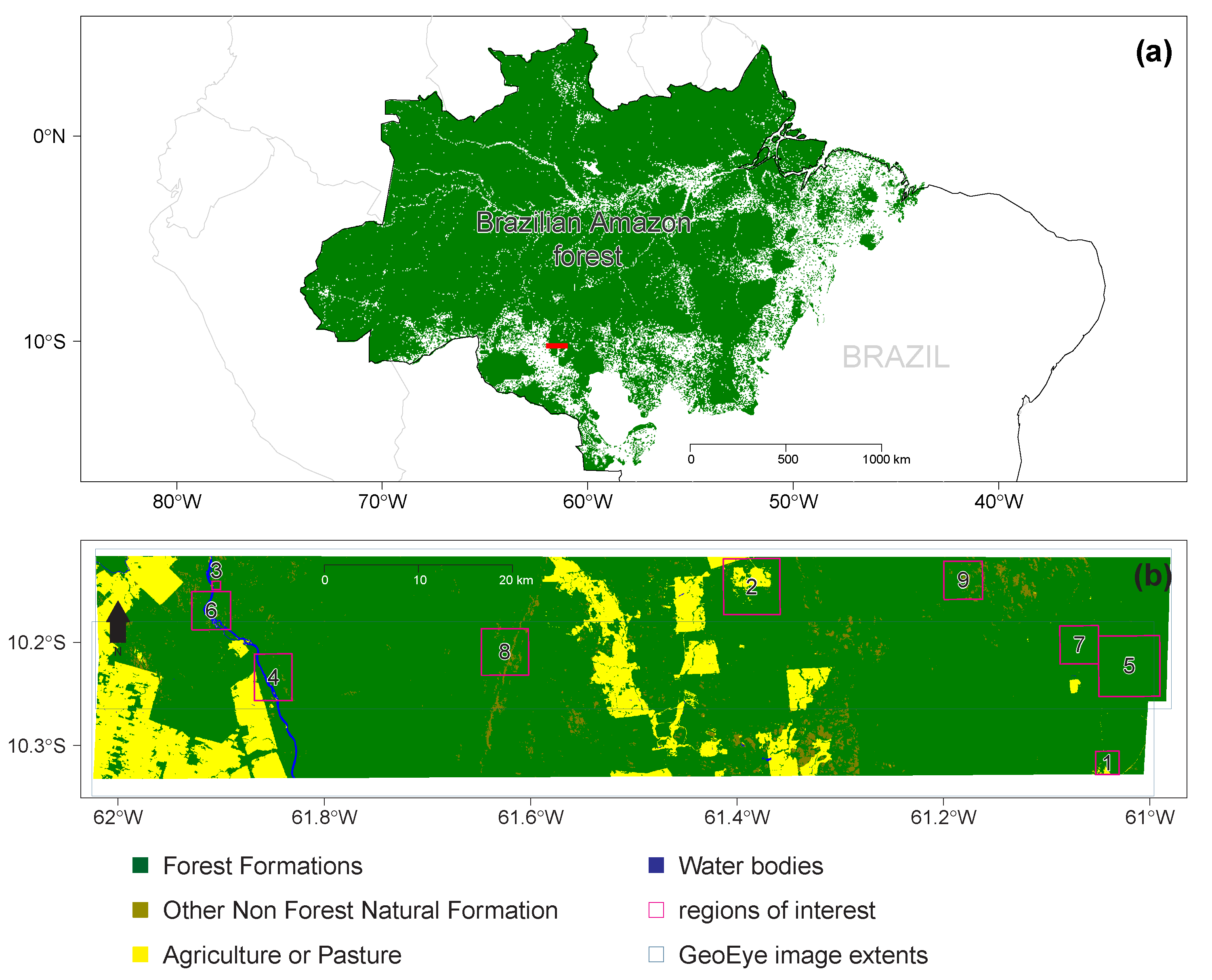
2.1. Study Region
2.2. GeoEye-1 Image
2.3. Forest Cover Mask and Clear-Cut Deforestation History from PRODES
2.4. Wetland Mask
2.5. Elevation Data
2.6. Statistical Analysis
3. Canopy Palm Segmentation Model
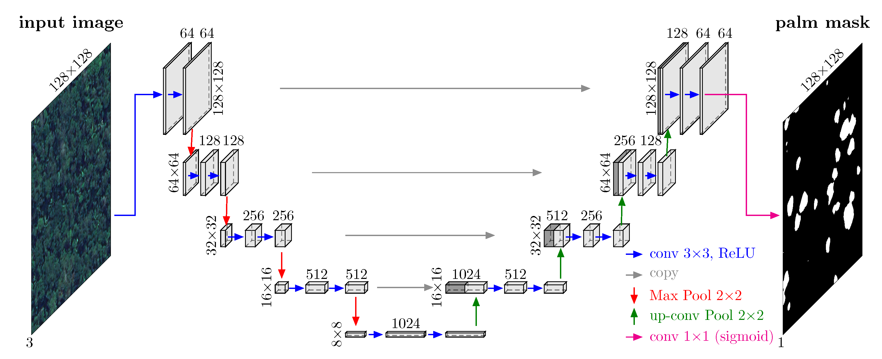
3.1. Model Architecture
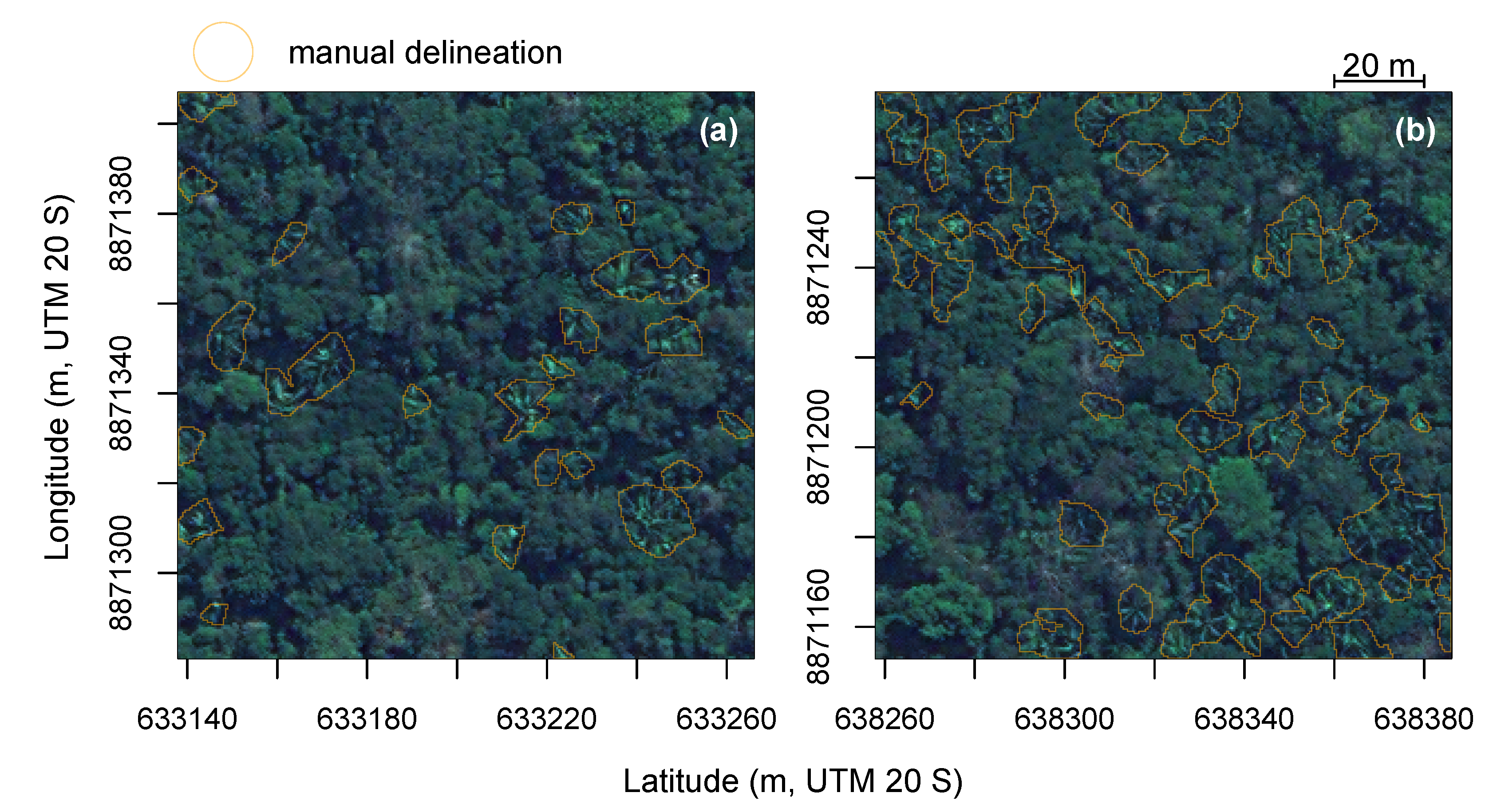
3.2. Canopy Palms Dataset
3.3. Model Training
3.4. Data Augmentation
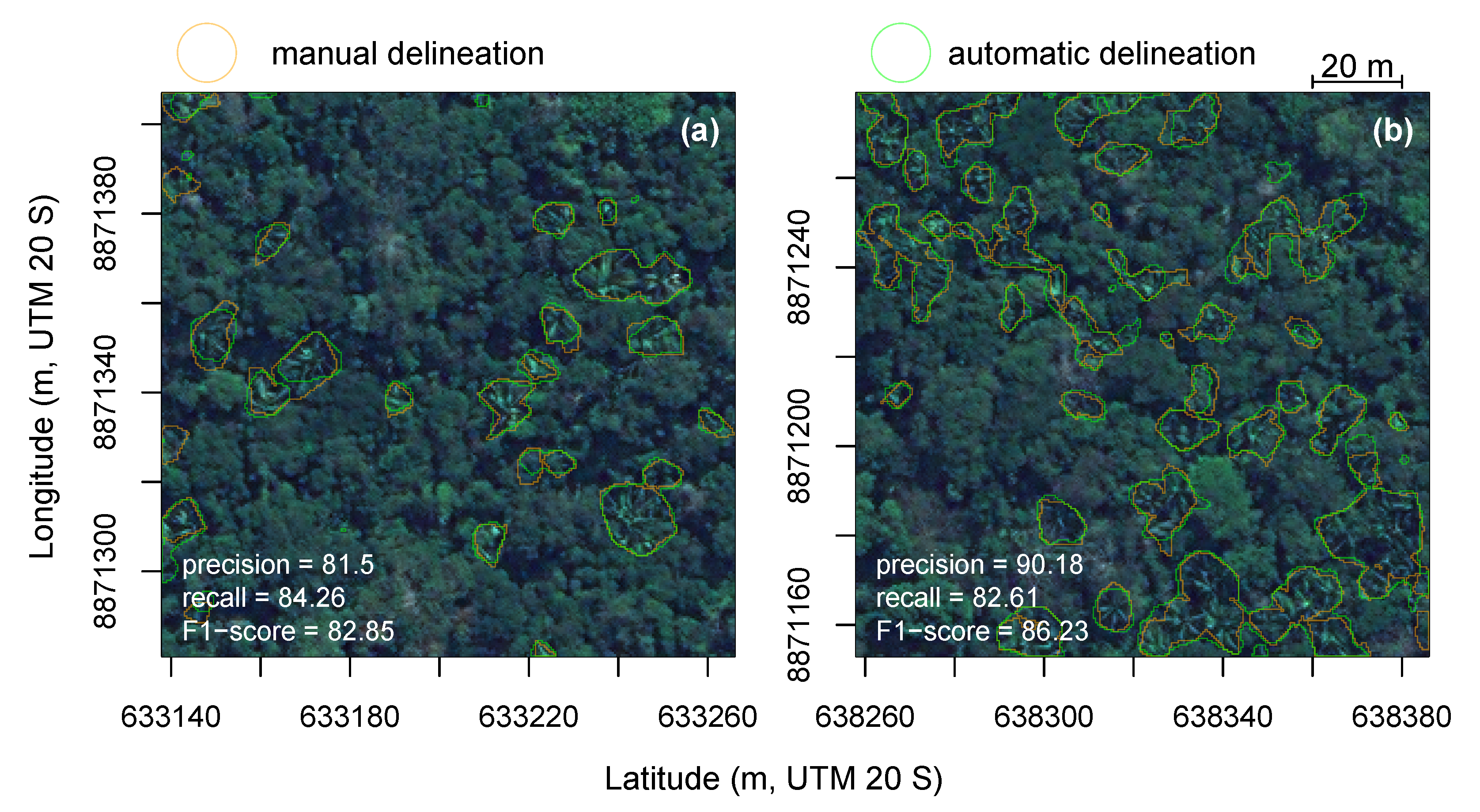
3.5. Segmentation Accuracy Assessment
3.6. Prediction
3.7. Algorithm
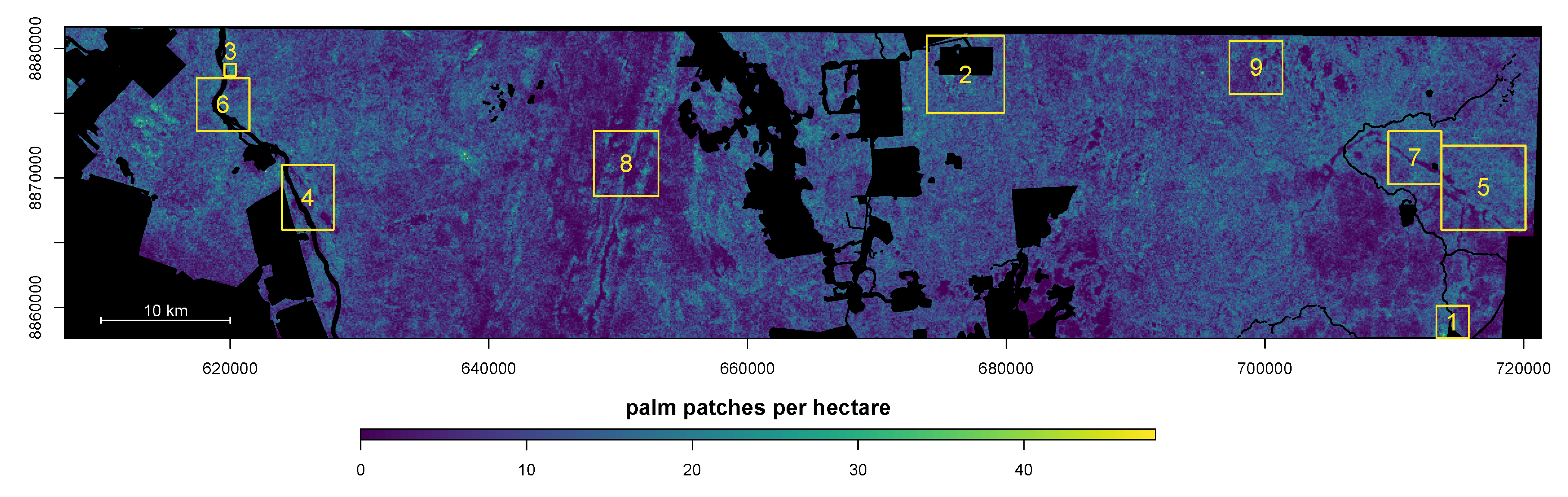
4. Results
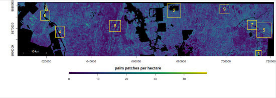
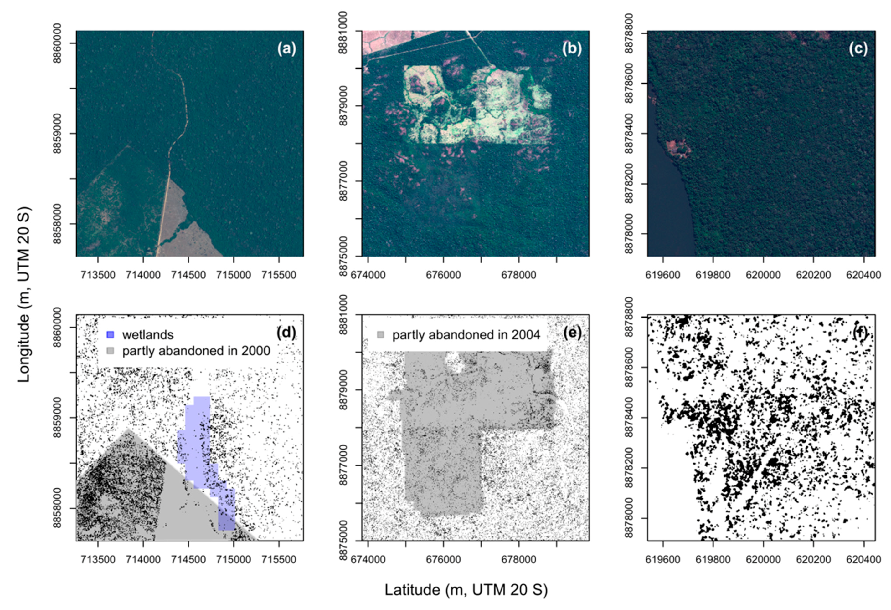
4.1. Distribution of Canopy Palms after Human Disturbances, Regions 1, 2 and 3
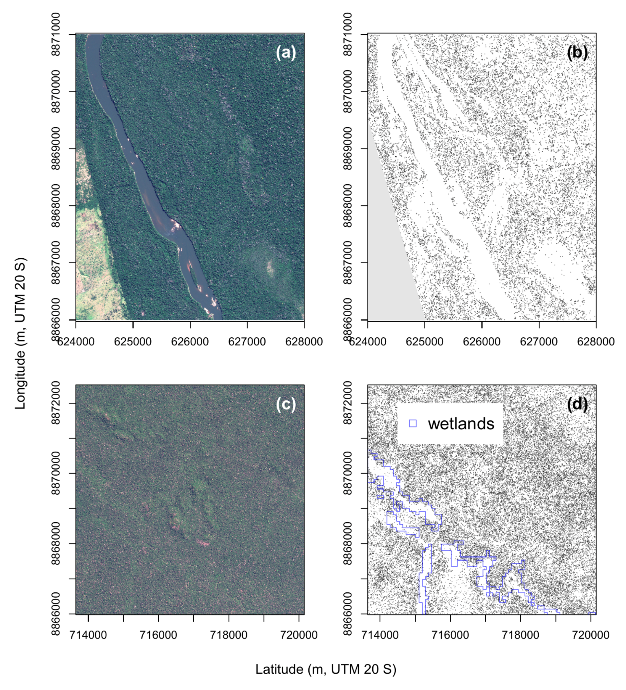
4.2. Natural Distribution of Canopy Palms near the River and Wetlands, Regions 4, 5, 6 and 7
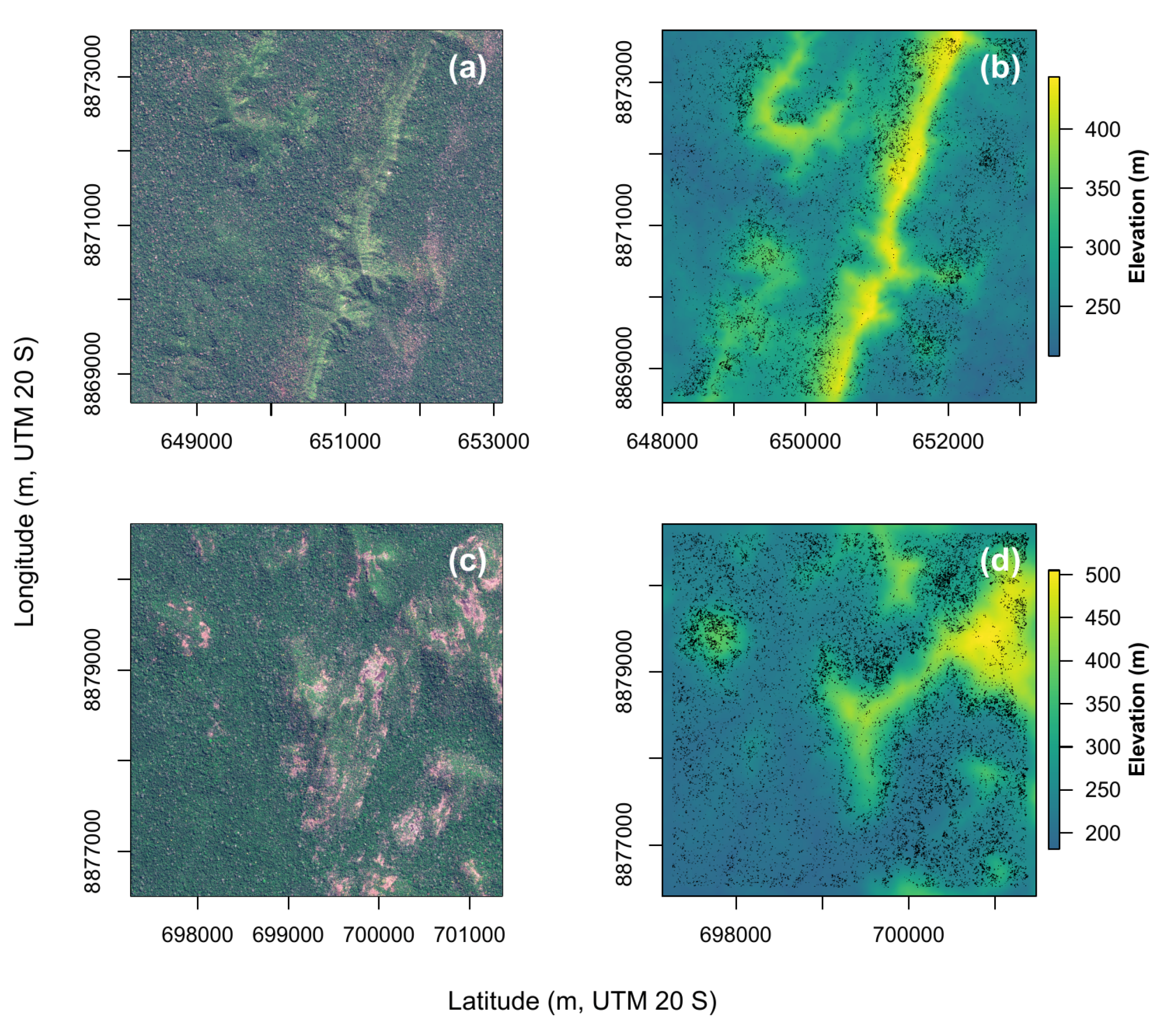
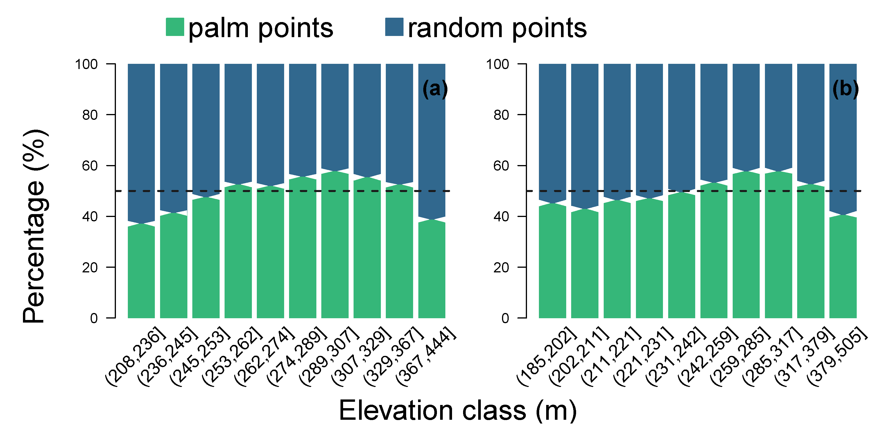
4.3. Natural Distribution of Canopy Palms at Higher Elevation Far from the Water Table, Regions 8 and 9
5. Discussion
5.1. Canopy Palm Mapping
5.2. Canopy Palm Distribution in Secondary Forests
5.3. Natural Spatial Distribution
5.4. Which Palm Species Are Observed?
6. Conclusions
Author Contributions
Funding
Acknowledgments
Conflicts of Interest
References
- Sutherland, W.J.; Freckleton, R.P.; Godfray, H.C.J.; Beissinger, S.R.; Benton, T.; Cameron, D.D.; Carmel, Y.; Coomes, D.A.; Coulson, T.; Emmerson, M.C.; et al. Identification of 100 fundamental ecological questions. J. Ecol. 2013, 101, 58–67. [Google Scholar] [CrossRef]
- Di Marco, M.; Ferrier, S.; Harwood, T.D.; Hoskins, A.J.; Watson, J.E. Wilderness areas halve the extinction risk of terrestrial biodiversity. Nature 2019, 573, 582–585. [Google Scholar] [CrossRef] [PubMed]
- Potapov, P.; Hansen, M.C.; Laestadius, L.; Turubanova, S.; Yaroshenko, A.; Thies, C.; Smith, W.; Zhuravleva, I.; Komarova, A.; Minnemeyer, S.; et al. The last frontiers of wilderness: Tracking loss of intact forest landscapes from 2000 to 2013. Sci. Adv. 2017, 3, e1600821. [Google Scholar] [CrossRef] [PubMed] [Green Version]
- Myers, N.; Mittermeier, R.A.; Mittermeier, C.G.; Da Fonseca, G.A.; Kent, J. Biodiversity hotspots for conservation priorities. Nature 2000, 403, 853. [Google Scholar] [CrossRef] [PubMed]
- Laurance, W.F. Conserving the hottest of the hotspots. Biol. Conserv. 2009, 142, 1137. [Google Scholar] [CrossRef]
- Slik, J.W.F.; Arroyo-Rodríguez, V.; Aiba, S.I.; Alvarez-Loayza, P.; Alves, L.F.; Ashton, P.; Balvanera, P.; Bastian, M.L.; Bellingham, P.J.; van den Berg, E.; et al. An estimate of the number of tropical tree species. Proc. Natl. Acad. Sci. USA 2015, 112, 7472–7477. [Google Scholar] [CrossRef] [Green Version]
- Ter Steege, H.; Pitman, N.C.; Sabatier, D.; Baraloto, C.; Salomão, R.P.; Guevara, J.E.; Phillips, O.L.; Castilho, C.V.; Magnusson, W.E.; Molino, J.F.; et al. Hyperdominance in the Amazonian tree flora. Science 2013, 342, 1243092. [Google Scholar] [CrossRef] [Green Version]
- National Institute for Space Research (INPE). Monitoring of the Brazilian Amazonian Forest by Satellite; Technical report; INPE, São José dos Campos: São José, Brazil, 2020; pp. 1988–2020. [Google Scholar]
- Mitchard, E.T.A.; Feldpausch, T.R.; Brienen, R.J.W.; Lopez-Gonzalez, G.; Monteagudo, A.; Baker, T.R.; Lewis, S.L.; Lloyd, J.; Quesada, C.A.; Gloor, M.; et al. Markedly divergent estimates of Amazon forest carbon density from ground plots and satellites. Glob. Ecol. Biogeogr. 2014, 23, 935–946. [Google Scholar] [CrossRef]
- Condit, R.; Ashton, P.S.; Manokaran, N.; LaFrankie, J.V.; Hubbell, S.P.; Foster, R.B. Dynamics of the forest communities at Pasoh and Barro Colorado: Comparing two 50–ha plots. Philos. Trans. R. Soc. Lond. B Biol. Sci. 1999, 354, 1739–1748. [Google Scholar] [CrossRef] [Green Version]
- Saatchi, S.; Mascaro, J.; Xu, L.; Keller, M.; Yang, Y.; Duffy, P.; Espírito-Santo, F.; Baccini, A.; Chambers, J.; Schimel, D. Seeing the forest beyond the trees. Glob. Ecol. Biogeogr. 2015, 24, 606–610. [Google Scholar] [CrossRef] [Green Version]
- Skidmore, A.K.; Pettorelli, N.; Coops, N.C.; Geller, G.N.; Hansen, M.; Lucas, R.; Mücher, C.A.; O’Connor, B.; Paganini, M.; Pereira, H.M.; et al. Environmental Science: Agree on Biodiversity Metrics to Track from Space. Nature 2015, 523, 403–405. [Google Scholar] [CrossRef] [PubMed] [Green Version]
- United Nations. Millennium Ecosystem Assessment, 2005. Ecosystems and Human Well-Being: Synthesis; Island Press: Washington, DC, USA, 2005. [Google Scholar]
- Brodrick, P.G.; Davies, A.B.; Asner, G.P. Uncovering Ecological Patterns with Convolutional Neural Networks. Trends Ecol. Evol. 2019, 34, 734–745. [Google Scholar] [CrossRef] [PubMed]
- Sánchez-Azofeifa, A.; Rivard, B.; Wright, J.; Feng, J.L.; Li, P.; Chong, M.M.; Bohlman, S.A. Estimation of the distribution of Tabebuia guayacan (Bignoniaceae) using high-resolution remote sensing imagery. Sensors 2011, 11, 3831–3851. [Google Scholar] [CrossRef] [PubMed]
- Kellner, J.R.; Hubbell, S.P. Density-dependent adult recruitment in a low-density tropical tree. Proc. Natl. Acad. Sci. USA 2018, 115, 11268–11273. [Google Scholar] [CrossRef] [PubMed] [Green Version]
- Wagner, F.H.; Sanchez, A.; Tarabalka, Y.; Lotte, R.G.; Ferreira, M.P.; Aidar, M.P.M.; Gloor, E.; Phillips, O.L.; Aragão, L.E.O.C. Using the U-net convolutional network to map forest types and disturbance in the Atlantic rainforest with very high resolution images. Remote Sens. Ecol. Conserv. 2019, 5, 360–375. [Google Scholar] [CrossRef] [Green Version]
- Wagner, F.H.; Sanchez, A.; Aidar, M.P.; Rochelle, A.L.; Tarabalka, Y.; Fonseca, M.G.; Phillips, O.L.; Gloor, E.; Aragão, L.E. Mapping Atlantic rainforest degradation and regeneration history with indicator species using convolutional network. PLoS ONE 2020, 15, e0229448. [Google Scholar] [CrossRef] [Green Version]
- Ronneberger, O.; Fischer, P.; Brox, T. U-Net: Convolutional Networks for Biomedical Image Segmentation. arXiv 2015, arXiv:1505.04597. [Google Scholar]
- Freudenberg, M.; Nölke, N.; Agostini, A.; Urban, K.; Wörgötter, F.; Kleinn, C. Large Scale Palm Tree Detection In High Resolution Satellite Images Using U-Net. Remote Sens. 2019, 11, 312. [Google Scholar] [CrossRef] [Green Version]
- Couvreur, T.L.; Forest, F.; Baker, W.J. Origin and global diversification patterns of tropical rain forests: Inferences from a complete genus-level phylogeny of palms. BMC Biol. 2011, 9, 44. [Google Scholar] [CrossRef] [Green Version]
- Eiserhardt, W.L.; Svenning, J.C.; Kissling, W.D.; Balslev, H. Geographical ecology of the palms (Arecaceae): Determinants of diversity and distributions across spatial scales. Ann. Bot. 2011, 108, 1391–1416. [Google Scholar] [CrossRef] [Green Version]
- Couvreur, T.L.; Baker, W.J. Tropical rain forest evolution: Palms as a model group. BMC Biol. 2013, 11, 48. [Google Scholar] [CrossRef] [PubMed] [Green Version]
- Mitja, D.; Ferraz, I.D. Establishment of babassu in pasture in Para, Brazil. Int. Palm Soc. 2001, 45, 138–147. [Google Scholar]
- Campos, J.L.A.; Albuquerque, U.P.; Peroni, N.; Araújo, E.d.L. Population structure and fruit availability of the babassu palm (Attalea speciosa Mart. ex Spreng) in human-dominated landscapes of the Northeast Region of Brazil. Acta Bot. Bras. 2017, 31, 267–275. [Google Scholar] [CrossRef] [Green Version]
- Junqueira, A.B.; Shepard, G.H.; Clement, C.R. Secondary forests on anthropogenic soils in Brazilian Amazonia conserve agrobiodiversity. Biodivers. Conserv. 2010, 19, 1933–1961. [Google Scholar] [CrossRef]
- Fraser, J.A.; Junqueira, A.B.; Kawa, N.C.; Moraes, C.P.; Clement, C.R. Crop diversity on anthropogenic dark earths in central Amazonia. Hum. Ecol. 2011, 39, 395–406. [Google Scholar] [CrossRef]
- McMichael, C.N.; Matthews-Bird, F.; Farfan-Rios, W.; Feeley, K.J. Ancient human disturbances may be skewing our understanding of Amazonian forests. Proc. Natl. Acad. Sci. USA 2017, 114, 522–527. [Google Scholar] [CrossRef] [Green Version]
- Tagle Casapia, X.; Falen, L.; Bartholomeus, H.; Cárdenas, R.; Flores, G.; Herold, M.; Honorio Coronado, E.N.; Baker, T.R. Identifying and quantifying the abundance of economically important palms in tropical moist forest using UAV imagery. Remote Sens. 2020, 12, 9. [Google Scholar] [CrossRef] [Green Version]
- Smith, N. Palms and People in the Amazon; Springer: Cham, Switzerland, 2014. [Google Scholar]
- Li, W.; Fu, H.; Yu, L.; Cracknell, A. Deep Learning Based Oil Palm Tree Detection and Counting for High-Resolution Remote Sensing Images. Remote Sens. 2017, 9, 22. [Google Scholar] [CrossRef] [Green Version]
- Guirado, E.; Tabik, S.; Alcaraz-Segura, D.; Cabello, J.; Herrera, F. Deep-learning versus OBIA for scattered shrub detection with Google earth imagery: Ziziphus Lotus as case study. Remote Sens. 2017, 9, 1220. [Google Scholar] [CrossRef] [Green Version]
- Zortea, M.; Nery, M.; Ruga, B.; Carvalho, L.B.; Bastos, A.C. Oil-Palm Tree Detection in Aerial Images Combining Deep Learning Classifiers. In Proceedings of the IGARSS 2018—2018 IEEE International Geoscience and Remote Sensing Symposium, Valencia, Spain, 22–27 July 2018; pp. 657–660. [Google Scholar]
- Mubin, N.A.; Nadarajoo, E.; Shafri, H.Z.M.; Hamedianfar, A. Young and mature oil palm tree detection and counting using convolutional neural network deep learning method. Int. J. Remote Sens. 2019, 40, 7500–7515. [Google Scholar] [CrossRef]
- Li, W.; Dong, R.; Fu, H.; Yu, L. Large-scale oil palm tree detection from high-resolution satellite images using two-stage convolutional neural networks. Remote Sens. 2019, 11, 11. [Google Scholar] [CrossRef] [Green Version]
- Neupane, B.; Horanont, T.; Hung, N.D. Deep learning based banana plant detection and counting using high-resolution red-green-blue (RGB) images collected from unmanned aerial vehicle (UAV). PLoS ONE 2019, 14, e0223906. [Google Scholar] [CrossRef] [PubMed]
- Ammar, A.; Koubaa, A. Deep-Learning-based Automated Palm Tree Counting and Geolocation in Large Farms from Aerial Geotagged Images. arXiv 2020, arXiv:cs.CV/2005.05269. [Google Scholar]
- Hofhansl, F.; Chacón-Madrigal, E.; Fuchslueger, L.; Jenking, D.; Morera-Beita, A.; Plutzar, C.; Silla, F.; Andersen, K.M.; Buchs, D.M.; Dullinger, S.; et al. Climatic and edaphic controls over tropical forest diversity and vegetation carbon storage. Sci. Rep. 2020, 10, 1–11. [Google Scholar] [CrossRef] [PubMed] [Green Version]
- Kristiansen, T.; Svenning, J.C.; Eiserhardt, W.L.; Pedersen, D.; Brix, H.; Munch Kristiansen, S.; Knadel, M.; Grández, C.; Balslev, H. Environment versus dispersal in the assembly of western Amazonian palm communities. J. Biogeogr. 2012, 39, 1318–1332. [Google Scholar] [CrossRef]
- Costa, F.R.; Guillaumet, J.L.; Lima, A.P.; Pereira, O.S. Gradients within gradients: The mesoscale distribution patterns of palms in a central Amazonian forest. J. Veg. Sci. 2009, 20, 69–78. [Google Scholar] [CrossRef]
- Feldpausch, T.R.; Banin, L.; Phillips, O.L.; Baker, T.R.; Lewis, S.L.; Quesada, C.A.; Affum-Baffoe, K.; Arets, E.J.; Berry, N.J.; Bird, M.; et al. Height-diameter allometry of tropical forest trees. Biogeosciences 2011, 8, 1081–1106. [Google Scholar] [CrossRef] [Green Version]
- MapBiomas. Project MapBiomas, Collection 2.3 of Brazilian Land Cover & Use Map Series; Technical report; MAPBIOMAS: São Paulo, Brazil, 2018; Available online: https://mapbiomas.org/en/o-que-e-o-mapbiomas (accessed on 1 September 2019).
- GDAL/OGR contributors. GDAL/OGR Geospatial Data Abstraction Software Library; Open Source Geospatial Foundation: Chicago, IL, USA, 2020. [Google Scholar]
- Grizonnet, M.; Michel, J.; Poughon, V.; Inglada, J.; Savinaud, M.; Cresson, R. Orfeo ToolBox: Open source processing of remote sensing images. Open Geospat. Data Softw. Stand. 2017, 2, 15. [Google Scholar] [CrossRef] [Green Version]
- QGIS Development Team. QGIS Geographic Information System; Open Source Geospatial Foundation: Chicago, IL, USA, 2009. [Google Scholar]
- Hess, L.; Melack, J.; Affonso, A.; Barbosa, C.; Gastil-Buhl, M.; Novo, E. LBA-ECO LC-07 Wetland Extent, Vegetation, and Inundation: Lowland Amazon Basin; ORNL DAAC: Oak Ridge, TN, USA, 2015. [Google Scholar]
- ALOS—PALSAR—JAXA/EORC ALOS PALSAR_Radiometric_Terrain_Corrected_high_res. JAXA/METI 2019, 11. [CrossRef]
- R Core Team. R: A Language and Environment for Statistical Computing; R Foundation for Statistical Computing: Vienna, Austria, 2016. [Google Scholar]
- Huang, B.; Lu, K.; Audebert, N.; Khalel, A.; Tarabalka, Y.; Malof, J.; Boulch, A.; Le Saux, B.; Collins, L.; Bradbury, K.; et al. Large-scale semantic classification: Outcome of the first year of Inria aerial image labeling benchmark. In Proceedings of the IEEE International Geoscience and Remote Sensing Symposium—IGARSS 2018, Valencia, Spain, 22–27 July 2018. [Google Scholar]
- Dice, L.R. Measures of the amount of ecologic association between species. Ecology 1945, 26, 297–302. [Google Scholar] [CrossRef]
- Allaire, J.; Chollet, F. keras: R Interface to ‘Keras’, R package version 2.1.4; GitHub; 2016. Available online: https://github.com/rstudio/keras (accessed on 1 September 2020).
- Chollet, F. Keras. Available online: https://keras.io (accessed on 1 September 2019).
- Abadi, M.; Agarwal, A.; Barham, P.; Brevdo, E.; Chen, Z.; Citro, C.; Corrado, G.S.; Davis, A.; Dean, J.; Devin, M.; et al. TensorFlow: Large-Scale Machine Learning on Heterogeneous Systems. 2015. Available online: tensorflow.org (accessed on 1 September 2019).
- Dalagnol, R.; Wagner, F.H.; Galvão, L.S.; Nelson, B.W.; Aragão, L.E.O.C. Life cycle of bamboo in the southwestern Amazon and its relation to fire events. Biogeosciences 2018, 15, 6087–6104. [Google Scholar] [CrossRef] [Green Version]
- Kahn, F.; De Granville, J.J. Palms in Forest Ecosystems of Amazonia; Springer Science & Business Media: Cham, Switzerland, 2012; Volume 95. [Google Scholar]
- Peters, C.M.; Balick, M.J.; Kahn, F.; Anderson, A.B. Oligarchic forests of economic plants in Amazonia: Utilization and conservation of an important tropical resource. Conserv. Biol. 1989, 3, 341–349. [Google Scholar] [CrossRef]
- Mitja, D.; Sirakov, N.; dos Santos, A.M.; González-Pérez, S.; Macedo, D.J.; Delaître, E.; Demagistri, L.; Loisel, P.; de Souza Miranda, I.; Rey-Valette, H.; et al. Viability of the Babassu Palm Eco-socio-system in Brazil: The Challenges of Coviability. In Coviability of Social and Ecological Systems: Reconnecting Mankind to the Biosphere in an Era of Global Change; Springer: Cham, Switzerland, 2019; pp. 257–284. [Google Scholar]
- Mesquita, R.C.; Ickes, K.; Ganade, G.; Williamson, G.B. Alternative successional pathways in the Amazon Basin. J. Ecol. 2001, 89, 528–537. [Google Scholar] [CrossRef] [Green Version]
- Wieland, L.M.; Mesquita, R.C.; Bobrowiec, P.E.D.; Bentos, T.V.; Williamson, G.B. Seed rain and advance regeneration in secondary succession in the Brazilian Amazon. Trop. Conserv. Sci. 2011, 4, 300–316. [Google Scholar] [CrossRef] [Green Version]
- Tomlinson, P.B. The uniqueness of palms. Bot. J. Linn. Soc. 2006, 151, 5–14. [Google Scholar] [CrossRef]
- Denevan, W.M. A bluff model of riverine settlement in prehistoric Amazonia. Ann. Assoc. Am. Geogr. 1996, 86, 654–681. [Google Scholar] [CrossRef]
- Clement, C.R.; Denevan, W.M.; Heckenberger, M.J.; Junqueira, A.B.; Neves, E.G.; Teixeira, W.G.; Woods, W.I. The domestication of Amazonia before European conquest. Proc. R. Soc. B Biol. Sci. 2015, 282, 20150813. [Google Scholar] [CrossRef] [Green Version]
- Svenning, J.C. On the role of microenvironmental heterogeneity in the ecology and diversification of neotropical rain-forest palms (Arecaceae). Bot. Rev. 2001, 67, 1–53. [Google Scholar] [CrossRef]
- Clark, D.A.; Clark, D.B.; Sandoval, R.M.; Castro, M.V.C. Edaphic and human effects on landscape-scale distributions of tropical rain forest palms. Ecology 1995, 76, 2581–2594. [Google Scholar] [CrossRef]
- Kahn, F. The distribution of palms as a function of local topography in Amazonian terra-firme forests. Exp. Basel 1987, 43, 251–258. [Google Scholar] [CrossRef]
- Vormisto, J.; Tuomisto, H.; Oksanen, J. Palm distribution patterns in Amazonian rainforests: What is the role of topographic variation? J. Veg. Sci. 2004, 15, 485–494. [Google Scholar] [CrossRef]
- Cámara-Leret, R.; Tuomisto, H.; Ruokolainen, K.; Balslev, H.; Munch Kristiansen, S. Modelling responses of western Amazonian palms to soil nutrients. J. Ecol. 2017, 105, 367–381. [Google Scholar] [CrossRef]
- Pimentel, D.S.; Tabarelli, M. Seed dispersal of the palm Attalea oleifera in a remnant of the Brazilian Atlantic Forest. Biotropica 2004, 36, 74–84. [Google Scholar] [CrossRef]


| Image Id | Palms Number | Palms per ha | Mean Size (m) | SD Size (m) | Median Size (m) | Minimum Size (m) | Maximum Size (m) | Forest Area (ha) | Palms Area (ha) | Palms Percent Prea (%) |
|---|---|---|---|---|---|---|---|---|---|---|
| P001 | 1,331,295 | 8.83 | 71.86 | 97.03 | 45.25 | 0.25 | 4200.25 | 150,766.11 | 9566.67 | 6.35 |
| P002 | 1,572,343 | 10.21 | 66.71 | 105.71 | 35.25 | 0.25 | 4977.25 | 153,967.32 | 10,489.85 | 6.81 |
| P001P002 | 2,147,750 | 9.51 | 67.50 | 102.16 | 38.00 | 0.25 | 4977.25 | 225,762.56 | 14,497.07 | 6.42 |
© 2020 by the authors. Licensee MDPI, Basel, Switzerland. This article is an open access article distributed under the terms and conditions of the Creative Commons Attribution (CC BY) license (http://creativecommons.org/licenses/by/4.0/).
Share and Cite
Wagner, F.H.; Dalagnol, R.; Tagle Casapia, X.; Streher, A.S.; Phillips, O.L.; Gloor, E.; Aragão, L.E.O.C. Regional Mapping and Spatial Distribution Analysis of Canopy Palms in an Amazon Forest Using Deep Learning and VHR Images. Remote Sens. 2020, 12, 2225. https://0-doi-org.brum.beds.ac.uk/10.3390/rs12142225
Wagner FH, Dalagnol R, Tagle Casapia X, Streher AS, Phillips OL, Gloor E, Aragão LEOC. Regional Mapping and Spatial Distribution Analysis of Canopy Palms in an Amazon Forest Using Deep Learning and VHR Images. Remote Sensing. 2020; 12(14):2225. https://0-doi-org.brum.beds.ac.uk/10.3390/rs12142225
Chicago/Turabian StyleWagner, Fabien H., Ricardo Dalagnol, Ximena Tagle Casapia, Annia S. Streher, Oliver L. Phillips, Emanuel Gloor, and Luiz E. O. C. Aragão. 2020. "Regional Mapping and Spatial Distribution Analysis of Canopy Palms in an Amazon Forest Using Deep Learning and VHR Images" Remote Sensing 12, no. 14: 2225. https://0-doi-org.brum.beds.ac.uk/10.3390/rs12142225