Article

Combining Satellite Multispectral Imagery and Topographic Data for the Detection and Mapping of Fluvial Avulsion Processes in Lowland Areas

1
Department of Earth Sciences, SAPIENZA University of Rome, 00185 Rome, Italy
2
Institute of Environmental Geology and Geoengineering (IGAG), National Research Council, 00010 Montelibretti (Rome), Italy
3
NHAZCA s.r.l., Spin-off SAPIENZA University of Rome, 00185 Rome, Italy
4
Department of Pure and Applied Sciences, University of Urbino “Carlo Bo”, 61029 Urbino (PU), Italy
5
Department of Ancient Sciences, SAPIENZA University of Rome, 00185 Rome, Italy
*
Author to whom correspondence should be addressed.
Remote Sens. 2020, 12(14), 2243; https://0-doi-org.brum.beds.ac.uk/10.3390/rs12142243
Submission received: 5 June 2020 / Revised: 7 July 2020 / Accepted: 8 July 2020 / Published: 13 July 2020
(This article belongs to the Special Issue Remote Sensing for Geomorphological Mapping)

Abstract

:
Fluvial avulsion is an important process in the dynamics of the riverscapes and plays a key role in the drainage network evolution in lowland areas, also influencing past and present social processes and economic activities. Crevasse splays represent significant geomorphological features for understanding the fluvial morphodynamics in lowland areas dominated by avulsion processes. Within wide floodplains characterized by very low elevation ranges, the detection and accurate mapping of crevasse splay morphology and features, such as crevasse channels, levees, and deposit, can be very challenging considering floodplain extension, anthropic impact on the natural channels network, logistic difficulties, and in some cases, climate conditions that prevent field work. This research aims at improving the detection and mapping of crevasse splays in lowland areas through the combination of different remote sensing techniques based on optical multispectral imagery and topographic data derived from satellite earth observation missions. The Lower Mesopotamia Plain (LMP) offers a unique opportunity to study the avulsion processes because it presents numerous examples of crevasse splays, characterized by different sizes and states of activity. Furthermore, in this area, a strong correlation exists between the formation and development of crevasse splays and the expansion of agriculture and early societies since the Early Holocene. Different supervised classification (SC) methods of Landsat 8 satellite images have been tested together with topographic analysis of the microrelief, carried out based on two different 1-arcsec DEMs (AW3D30 and GDEM2). The results of this study demonstrate that the combination of multispectral imagery analysis and topographic analysis of the microrelief is useful for discerning different crevasse elements, distinguishing between active and relict landforms. The methodological approach proved helpful for improving the mapping of erosional and depositional landforms generated by the avulsion process and, in the study area, provided the best results for the active landforms.

1. Introduction

The fluvial avulsion represents a periodic process in the morphoevolution of the floodplains and consists of an abrupt shift of the whole channel belt from one location to another, favouring the formation of a new watercourse [1,2,3,4,5,6]. This process mainly occurs during flood events and requires the bed of the new course being topographically lower than the old channel belt [4,6]. This implies a supra-elevation of the older channel belt above the floodplain, a condition that requires net aggradation of the channel for a long period of time [7]. As the inception of the avulsion process requires an energetic water flow, it is quite logical to consider this process connected with the widening of a channel on a crevasse splay, although the intersection of the main channel with an existing channel can favour avulsion [6]. So, crevasse processes and deposits and their associate landforms represent important geomorphological features for understanding the fluvial morphodynamics in lowland areas, and provide evidence for the mechanism of avulsion [5,8,9,10,11,12,13,14,15].
A crevasse splay typically shows a lobate sediment accumulation area, fan shaped in plan with an upward convexity and contain a system of distributive multi-channels system [16]. The fluvial avulsion begins and develops when flooding waters break through a high-topographic levee at the time of peak flood discharge or when the bankfull discharge overtops the levees. The sediment deposition occurs when the flow decelerates, passing from confined to unconfined conditions (i.e., from distributive crevasse channels in the proximal sector to lobe deposits in the middle and distal sectors), or when the flooding water enters a standing waterbody [15,17,18,19]. The crevasse splay deposits usually consist of very fine to medium-grained sands. These deposits are coarser and thicker in the proximal portion, where sharp and erosional-based structureless or medium-scale cross-bedding (dune) sand units occur (channel-bar and channel-fill deposits). Finer and thinner deposits occur in the middle and distal sectors, where cross-laminated sand (essentially climbing-ripples strata) with load structures pass downcurrent to structureless finer sand and silt deposits, and finally to the floodbasin mudstone [4,6,18,20]. Generally, these deposits are vertically organized, forming coarsening to fining upward successions that reflect the increase and the decrease of flood energy during deposition. The variation of grain-size both parallel and perpendicular to flow direction (i.e., across strike and down dip) is attributed to the decrement of floodwater energy, which is in turn related to flow expansion away from the crevasse channel [18,20]. All these processes develop during the life cycle of a crevasse splay [19] in which the floodplain gradient plays a relevant role. It acts, in fact, as the base level for the crevasse channels, adjusting towards a graded equilibrium profile. Therefore, at the beginning of the cycle, the outflow of floodwater promotes erosion near the proximal sector and deposition in the middle and distal sectors of the crevasse splay [19]. The continued erosion in the crevasse proximal suggests that this sector essentially represents a by-passing zone, that becomes a depositional zone during the waning stage of flooding. When the return flow of floodwater allows sediment deposition into the crevasse channels (backfilling), a decrease of the floodplainward gradient occurs, deactivating the crevasse splay [19]. All these data evidence that a crevasse splay is a composite body, made up of stacked vertically and laterally single splays deposited by single flooding events and organized with a typical progradational trend [19,20]. These composite bodies are generally 3–4 m thick, up to 10 km long and 5 km wide, and may reach several square kilometres [17,18,20], depending generally on sediment grain-size and floodplain-drainage conditions [19,21]. Crevasses are particularly important landforms of the anastomosed fluvial environment, as their formation represents an intermediate step in the avulsion of the main channels into new positions on the floodplain [15,19]. The floodplain sectors surrounding crevasse splays were the zones where the earliest human settlements established and developed. An outstanding example is the Mesopotamian Plain (hereafter MP) where, thanks to the fluvial avulsion process and the development of the associated landforms, the Akkadian civilization found the ideal conditions for introducing the first agricultural techniques [22].
In order to identify Earth surface processes and associated landforms and, eventually, correlated archaeological and anthropic features, especially where political conflicts/warfare occur or the climate conditions prevent detailed fieldworks, the use of remote sensing techniques give a relevant support ([23,24,25,26,27,28,29] and references therein). Moreover, wide extensions of the areas under investigation encourage the application of these techniques. Remote sensing and multispectral imagery have notable potential for detecting changing fluvial systems and reconstructing the drainage networks in areas characterized by low topographic relief, especially when landforms are no longer visible on the ground, such as those belonging to relict waterscapes [23,30]. In particular, for detecting processes and landforms within lowland areas, the exclusive use of remote sensing techniques based on digital elevation datasets can be difficult.
The aim of this study is the application of a combination of different remote sensing techniques for detecting typical landforms association due to the fluvial avulsion process, such as crevasse splays. We use the Lower Mesopotamian Plain (hereafter LMP) as a test site, being an ideal place to apply and verify such a combined approach due to data availability, landscape configuration, and the presence of a well-developed example of active and relict landforms due to the fluvial avulsion process. Indeed, both the occurrence of active and relict crevasse splays and the semi-arid morphoclimatic context with scattered vegetation cover make the LMP an exemplary study area. A visual interpretation of both Google® Earth and TerraColor satellite imagery datasets have been performed for preliminarily detecting and mapping crevasse splays over the LMP, verifying those landform datasets already available in literature for the area [31,32,33]. Terrain analysis based on topographic data from satellite has been successively performed for the study of the microrelief in selected sites. Finally, multispectral analysis and different methods of supervised classification have been carried on Landsat 8 optical imagery. Remote sensing data serves two main goals: (1) detecting and mapping the association of different active erosional and depositional landforms due to the fluvial avulsion process (i.e., rivers, levees, floodplain, crevasse splays); (2) detecting and mapping relict landforms, such as abandoned river courses, levee breaks, and associated inactive crevasse splays.

2. Study Area

The LMP is the southernmost sector of the MP, a rather flat area with a low topographic relief comprised between the latitude of 32°30′00″ N and 29°50′00″ N. LMP is bordered by the Zagros Mountains to the north-east and by the Arabian Desert to the west (Figure 1). The Tigris and Euphrates rivers are the main watercourse, occupying the marginal sectors of the Mesopotamian alluvial plain both with a northwest-southeast flow direction, parallel to the plain axis [34]: the Euphrates flows in the western side while the Tigris in the eastern sector. These rivers join near Basra, forming the Shatt-Al-Arab River, which mouths in the Persian Gulf, after about 170 km, forming an estuary with a wide marshland area [34,35]. Fluvial processes mainly characterize the entire LMP and many active and relict fluvial landforms widely occur in the area [31,34,36,37]. Fluvial avulsion was relevant for the development of the Mesopotamian civilization [31] and the evolution of such a fluvial process is due to different processes: (i) annexation, whereby an existing channel is (re-)occupied; (ii) diversion, through which a flow is deviated into the adjacent flood basin with the consequently deposition of a sediment wedge expanding downstream; (iii) incision, whereby a new channel is scoured in the floodplain [5,38].
The Quaternary deposits cover the totally of the MP and are mainly represented by clastic sediments (from gravel to clay) derived by the erosion of the Zagros Mountains and the Arabian Platform [39] and mainly delivered by the Tigris and Euphrates rivers and their tributaries. Although fluvial sedimentation is at present the main active process within the plain, due to the Quaternary climate change and glacio-eustatic sea-level oscillations, several environments were active, giving rise to different depositional units characterized by fluvial, deltaic, lacustrine, estuarine, marine and aeolian deposits [40,41,42]. The most recent sediments are Early-Mid Holocene in age and were deposited during the last post-glacial sea-level rise. This process produced a general landward and northward migration of the Persian Gulf shoreline to which followed, during Late Holocene, a seaward migration of the shoreline due to the Tigris and Euphrates delta progradation [43,44,45,46,47,48]. In detail, from the peak of the last glaciation until about 14,000 yrs BP (Late Pleistocene), the Persian Gulf was completely in sub-aerial condition. From 14,000 to 9,000 yrs BP (Late Pleistocene–Early Holocene) with the rapid sea-level rise, the Gulf was flooded, and a wide fluvial system developed in the area. Consequently, during the shoreline transgression, the existing valley was flooded and transformed in an estuary, where fluvial and tidal processes were active [49,50]. The present shoreline was reached about 7000–8000 yrs BP [44]. About 6000 yrs BP (Mid Holocene), the shoreline was at the maximum inland ingression; its position is still highly debated [48], although several studies suggest its location in the sector between the modern cities of Nasiriyah and Amarah [45,46,47,51,52], where the Tigris and Euphrates rivers gave rise to the formation of well-developed river-dominated deltas [47]. Deltaic progradation was rapid between 6000 and 4000 yrs BP, due to the wetter climate conditions, whereas it slowed significantly between 4000 and 3000 yrs BP because of the increase in aridity [45,46]. The decrease of the Tigris and Euphrates rivers sediment supply, together with climate change and tectonic movements, produced a physiographic change of the area that was transformed in a marshy environment, and freshwater conditions persisted since about 3000 yrs BP [41,45]. The Gulf probably attained its present configuration around 1000 AD as a result of the construction of the Shatt-Al-Arab delta.
Over the hydrological year, there are two major flooding peaks: November–March due to the immediate surface runoff, and April–May chiefly related to snowmelt. Instead, the summer season is broadly characterized by a decrease of rainfalls and river discharge [34,37]. Thus, the interannual discharge variability ranges from 1.9–6.3 × 10¹⁰ m³ for the Tigris, and 1.0–3.6 × 10¹⁰ m³ for the Euphrates, according to the measurements collected between 1924 and 1946, during the relatively unaltered streamflow [37].
The LMP waterscape is characterized by several active and abandoned fluvial landforms, such as active and abandoned channels of meandering and anastomosing river patterns, abandoned channels belonging to a paleo-delta distributary system, levees above the surrounding floodplains and widespread active and relict crevasse splays [31,34,36,37]. The long settlement history of this region caused a relevant alteration of the hydrological and sedimentary processes through the flood management and water supply techniques [33,36,38,53,54,55]. Man-made canals and archaeological sites are detectable in the study area, especially through their relative elevation above the surrounding flat floodplain [56].
Despite many engineering works for the management of the drainage network dynamics, avulsion processes are rather widespread in the study area, mainly due to the discharge variability and the high floods [31]. Hence, obtaining deeper insights into this fluvial process and its associated landforms, such as crevasse splays, represents an important issue for river engineers to prevent catastrophic events [38].

3. Materials and Methods

Combined remote sensing techniques which integrate data derived from different earth observation missions, have been applied in the present research. The methodological approach provided a preliminary visual inspection to support topographic data and optical multispectral imagery analysis.

3.1. Preliminary Inspection

For the preliminary recognition of possible landforms assemblage due to the fluvial avulsion, in particular crevasse deposits, channels, and levees, a visual inspection and interpretation has been performed on the optical satellite imagery freely available in the Google® Earth virtual globe and the ESRI® TerraColor dataset, included in the ESRI® ArcGIS 10.6 software package. This preliminary study allowed an early discerning of active fluvial landforms and of the present-day channels network mainly characterised by irrigation systems superimposed to the natural channel systems [33,34,37,38,46]. Google® Earth virtual globe includes the first satellite optical database with a time-lapse overview over the period 1984–2016 with a maximum geometrical resolution of 2.5 m (i.e., SPOT imagery). Moreover, the optical dataset has been enhanced by the World Imagery layer in ArcGIS 10.6, recently updated with a more distinctive and more natural look TerraColor NextGen imagery from Earthstar Geographics [57]. World Imagery provides at least one-meter satellite and aerial imagery in many parts of the world and lower resolution satellite imagery worldwide. For the study area, the map includes 15 × 15 m TerraColor imagery at small and mid-scales and 2.5 × 2.5 m SPOT Imagery [58]. The typical distributary and anastomosing patterns of the crevasse channels were the main planform feature that allowed for their preliminary recognition of the crevasse splays over the whole LMP, combined with the association to the characteristic fan-shaped planar geometry of the crevasse deposits. Moreover, the roughly perpendicular development of the crevasse splays relative to the main watercourse, especially in the outer bank of meanders (Figure 2) revealed useful in this preliminary recognition.
Comparing different optical features, such as pattern, shape and height, is essential to recognize a crevasse splay, especially on optical imagery [36]. The dataset recognized in the study area also includes the crevasse splays already identified by previous authors [31,32,33].

3.2. Topographic Analysis of the Microrelief

For the analysis of the microrelief two different digital elevation datasets have been used, based on two freely available 1 arcsec, optical derived DEMs. The first dataset derives from the Panchromatic Remote-sensing Instrument for Stereo Mapping (PRISM) on board the Advanced Land Observing Satellite (ALOS) available at https://www.eorc.jaxa.jp/ALOS/en/aw3d30/index.htm (also known as AW3D30). The second dataset is the ASTER Global DEM (GDEM2) available at https://search.earthdata.nasa.gov/search, representing an average of different images collected between 2000 and 2011 [59]. The use of two different elevation datasets allowed for enhancing the reliability of the topographic elaborations through the comparison and mutual confirmation of different sources. This procedure is mandatory in the lowland areas where digital elevation data can really present many artefacts and/or systematic errors due to the scarce elevation range. Both DEMs used have a ground resolution of about 30 m.
The analysis and interpretation of the microrelief was favoured by the generation of colour-coded DEMs with a 1–5 m re-classification scheme starting from the sea-level up to the maximum elevation of the study area (with a major interval frequency for the first 30 m a.s.l.). In particular, taking into account the vertical accuracy of the AW3D30 [59,60] and the GDEM2 [59,61], a re-classification of the elevation data using narrow elevation intervals was helpful for the visual inspection of the floodplain features, even those landforms characterized by low or very low topographic relief. Specifically, 1-m interval re-classified DEMs lead to better visualize the higher elevation of the crevasse deposits relative to the surrounding floodplain, the higher elevation of the channel levees [56], as well as to emphasize the visualization of their planform convex geometry.
In order to find topographic and morphological differences between active and abandoned crevasse splays, four elevation profiles have been drawn using both elevation datasets. The first profile is along the dip direction, proximal to the adjacent floodplain, to evaluate the limit of distal crevasse deposits, while further profiles are along the cross direction in the proximal, middle, and distal sectors of the crevasse. In this way, the floodplainward loss of thickness can be appreciated along both dip and cross directions. Due to the use of optical-derived DEMs, the elevation profiles are affected by “on-surface noise” because of acquisition limits due to the presence of the vegetation cover, though scarce and scattered in this specific study area. Thus, the moving average filter has been applied for smoothing the elevation data.

3.3. Multispectral Satellite Imagery Analysis

It has long been known that alluvial fan surfaces of different ages can be distinguished using multispectral imagery [24,62,63]. Indeed, different reflectance properties in deposits with different ages have been attributed to changes in chemistry, mineralogical composition and microrelief as a result of weathering [24,62,64]. Therefore, multispectral imagery can be used to get information about the types of sedimentary deposits characterizing the crevasse fan surfaces [24]. Due to the availability of multispectral Landsat 8 satellite imagery for the LMP, a multispectral analysis and supervised classifications have been carried on.
Landsat 8 is an American Earth observation satellite launched on February 11, 2013. First known as Landsat Data Continuity Mission (LDCM), it was created for investigating and researching feasible solutions to follow Landsat 7 mission. Since 1972, Landsat satellites have continuously acquired images of the Earth’s land surface, providing uninterrupted data until today. Landsat 8 carries the Operational Land Imager (OLI) and the Thermal Infrared Sensor (TIRS). OLI works on nine spectral bands, including a panchromatic one, while TIRS works on the last two bands [65,66,67]. Besides its brief time life, Landsat 8 is one of the best multispectral satellites thanks to the eleven bands with high-resolution [63,64,65].
The dataset for the multispectral analysis includes the image tiles displayed in Figure 3. Considering the climatic regime of the LMP, two periods characterised by opposite moisture conditions have been selected including the wettest season (October–December) and the driest one (July–August). Consequently, the selected dataset presents different conditions of reflectance because of the variation in soil moisture, vegetation cover, and percentage of suspended materials along watercourses, but the clearness of the selected imagery allows for the proper interpretation of Earth surface landforms and processes.
The multispectral analysis has been carried on through the ENVI 5.3 software, on which the six tiles reported in Figure 3 have been firstly mosaicked, obtaining two mosaics for the wettest and driest periods, respectively.
The Spectral Indices Toolbox available in ENVI 5.3 leads to compute the Normalized Difference of Vegetation Index (NDVI), in order to assess the seasonal vegetation variability, the lateral shifting degree of crevasse channels, and to identify the areas where human activities have a lesser impact. Indeed, NDVI values indicate the amount of green vegetation occurring in each raster pixel and help to discern those areas where crops and human activities have obliterated the ancient landforms. Moreover, the development of vegetation drives the kind of overbank flow (i.e., confined vs unconfined) [68]. The presence of vegetation generally increases velocities within the confined channel, while the lateral outflow occurs due to the decreasing vegetation roughness [69]. The topography establishes a lateral water surface gradient between the channel and the islands even with low vegetation roughness, which drives lateral flow. Hence, the NDVI computation leads to focus on areas where inactive crevasse splays are better preserved and human activities do not occur.
The second spectral index computed is the Clay Ratio (CR), which highlights hydrothermally altered rocks containing clay and alunite. It is essential for recognizing the activity of crevasse channels and to infer the in-channel flow direction (i.e., floodplainward or riverward). During a flood event, the sand fraction transported as bedload is deposited especially in the proximal part of the splay, whereas the silt and clay fraction is transported in suspension to be deposited in the distal parts, where flow rates are reduced [18]. The return flow after a flooding event leads to the in-channel deposition of suspended sediment [19], potentially detectable through the CR.
Finally, specific target features have been submitted in the Supervised Classification (SC). In particular, in order to recognize crevasse splays and for focusing exclusively on them, the target features are delineated like Regions Of Interest (ROIs). The target feature of a crevasse splay has been distinguished into three main sub-features in order to better specify the ROIs, where the spectral signature has been extracted: (i) active and abandoned channel; (ii) active levee; (iii) active and abandoned deposit. The ROIs have been extracted on the active C10 and the abandoned C2, which sub-features are perfectly recognizable; the calibration ROIs for the SC are composed by 22 records for both the wettest and the driest periods. In the SC, four different methods have been adopted and their performance has been estimated: (1) Mahalanobis; (2) Maximum Likelihood; (3) Minimum Distance; (4) Spectral Angle Mapper (SAM) [70]. Different iterations have been done varying the specific thresholds for each classification method, but only the most accurate results have been described and discussed in this study. Despite the unavailability of a definite method to assess the absolute accuracy of image classification for remote sensing Earth observation applications, the computation of a confusion matrix is a widely accepted method to determine the relative accuracy of classifications, using the previous identified ROIs for ground truth [71]. Each element in the major diagonal of the confusion matrix represents the number of pixels that are correctly classified for a class x, whereas the elements out of the major diagonal are the number of pixels that should be in class x but which are incorrectly classified as class y. Certainly, if all the image pixels are correctly classified, we should then have a diagonal confusion matrix where all non-diagonal elements become zero [70,71]. The confusion matrix gives back the Overall Accuracy (OA) and the Kappa coefficient (K). The first one is the percentage of the correct classification and the second one is the statistical measure of classification accuracy and quality. The maximum value of K is 1, representing the perfect agreement between the classification and the reference data, while K becomes 0 for no agreement [71]. In light of the discouraged use of the Kappa metric in the remote sensing community for validating a classification [72], the User Accuracy (UA) and the Producer Accuracy (PA) have also been taken into consideration. The first one is the probability that a value predicted to be in a class x really is in that class, (i.e., how often the class x on the map occurs on the ground). The PA is the probability that a value in a given class was classified correctly, signifying how often the real features on the ground are correctly shown on the classified map [73,74]. The UA and PA for any given class usually are not the same. Figure 4 shows an example where the 75% of the crevasse channels occurred on the ground have been correctly classified (i.e., PA = 75%) whereas some of them are wrongly classified as “levee”. Anyway, the class “crevasse channel” perfectly corresponds to the channels on the ground, except for a “fake-channel” on the right side, thus only the 90% of the classified areas as “active channel” are actually a channel (i.e., UA = 90%) [75].
The assessment of accuracy leads to define which thresholds must be adopted for the most accurate classifications of crevasse features (Table 1).
The methodological scheme adopted in this research has been summarized in Figure 5.

4. Results

Results obtained in the study area are summarized in the following sections. The first section reports the results derived from the preliminary inspection and the topographic analysis carried out exploiting the elevation datasets. The second section reports the results from the multispectral analysis.

4.1. Preliminary Inspection and Topographic Analysis of the Microrelief

The preliminary inspection of the Google® Earth and TerraColor imagery allowed to identify several crevasse splays, either along the active fluvial system, especially on the right bank of the Tigris Rivers, or along abandoned channels. In the present research, four examples of crevasse splays have been selected based on their size (> 50 km2) and their state of activity (two examples among the recognized active crevasses and two among the abandoned ones). The preliminary inspection leads to identify the abandoned Kut-Al-Hayy East airbase in the middle-distal sector of C9. The area of this airbase is about 18 km2 and occupies only the 25% of the entire C9, with a negligible “noise” in the analysis of the entire landform (Figure 6). The multi-channel system, typical of crevasse splays, is the most recognizable feature in the optical imagery and its identification favoured the planar delimitation and mapping, especially for the active forms (Figure 6). The topographic analysis really improved the preliminary mapping favoured by the relevant differences in spatial distribution of the deposits between active and abandoned crevasse splays considering the along-dip and cross directions (Figure 6 and Figure 7). Moreover, the topographic analysis leads to a preliminary estimate of the depth of the deposits through the projection of the floodplain backward, up to the proximal sector of each along-dip section.
Authors should discuss the results and how they can be interpreted in perspective of previous studies and of the working hypotheses. The findings and their implications should be discussed in the broadest context possible. Future research directions may also be highlighted.
Indeed, among the recognized active crevasses, those named C10 and C13 (Figure 6) are located along the Tigris Rivers, but their shape and spatial development are deeply different. The first one has mainly dip-direction extension while C13 is substantially developed along the cross-direction. The same divergence can be appreciated in the elevation data. Generally, both crevasses show along-dip sections with an emphasized convex-up profile at the proximal sector, gradually flattening floodplainward. On the contrary, the cross-sections show the notable differences between C10 and C13 due to the different activity of their crevasse channels and the relative distribution of sediments (Figure 8). While C10 points out a more homogeneous channel activity and spatial distribution of sediments (Figure 8A), the proximal and middle cross-sections BB’ and CC’ of C13 display the main active channels in the southern part (Figure 8B). Anyway, each cross-section at the proximal, middle, and distal sectors broadly display the progressive decrease floodplainward of the crevasse deposits thickness (Figure 8). The thickness of C10 and C13 deposits are quite different: in C10, the proximal deposit is about 2.5 m thick, the middle deposit is 3 m, and the distal one reaches the lowest thickness with 1.5 m, while in C13, the proximal deposit is thicker (about 3 m), the middle deposit is about 2 m thick, and the distal deposit is quite similar to the C10 one.
The two examples of abandoned crevasse splays, here named C2 and C9 present, as expected, rather different geomorphological and geometric characteristics with respect to the active crevasses before described. C2 is well recognizable mainly in dip-section, while the cross-sections do not preserve the typical convex-up shape (Figure 9A). C9 shows a less convex-up profile of the deposit in the along-dip and the cross-section CC’ (Figure 9B). Both C2 and C9 proximal deposits show a low thickness of about 1–2 m, the middle deposits are thicker reaching 3.5–4 m, while the distal deposits are 1.5–2 m thick. Nevertheless, a significant difference can be appreciated in the along-dip sections: the active crevasses C10 and C13 have an elevated proximal sector, directly connected to the above-floodplain levee of the parent channel (i.e., the Tigris River). On the contrary, the proximal sector of abandoned crevasse C2 shows a low elevation, seemingly disconnected to the abandoned Khalid channel, while C9 still preserves the above-floodplain elevation of the Dujaila channel.

4.2. Multispectral Satellite Imagery Analysis

4.2.1. NDVI and CR

The computation of the NDVI index and the CR improved the identification of crevasse splays, especially assessing the mobility of crevasse channels, the spatial distribution of the finest sediment and comparing the channelized/unchannelized flow. The NDVI has been classified into five classes (the lowermost value without a color) (Figure 10). In this way, the vegetation cover is highlighted in the areas where is more abundant and with a higher density, as for example along the riverbanks, within the croplands, and at crevasse splays. The NDVI does not discern which kind of vegetation we are looking (i.e., crops, riverine vegetation, or marshland), although the highest values have been recognized in the marshland areas.
The most evident difference in the NDVI computation is the occurrence of vegetation on active and abandoned crevasses, leading to discern their state of activity. Bearing in mind the influence of rainfall seasonality, the most reliable results were obtained with the images of the wettest period. Nevertheless, both examples of active crevasses (i.e., C10 and C13) show higher NDVI value than the abandoned ones (i.e., C2 and C9). Indeed, considering the NDVI during the wettest period, the highest values occur along the crevasse channels in the proximal and middle sectors of C10 (Figure 10). Otherwise, the NDVI values are higher in the southern part of C13, where the crevasse channels are largest. The occurrence of vegetation in the abandoned C2 and C9 is mainly due to the crops and human canals surrounding the crevasses.
The state of activity of crevasse channels is estimated also through the CR, which is classified into fifteen classes for the wettest period (Figure 11). As for the NDVI, the lowermost class has not a colour for emphasizing the areas with a higher clay content. This index is useful to recognize the in-channel clay like the last deposits of a flood event, when the floodwater goes back toward the parent channel due to the decrease of river discharge below the bankfull capacity. Anyway, the basinward overland flow could be captured into the crevasse channels or remnant depressions, like in C10, depositing the finest suspended load. The highest values of CR are also on the banks of crevasse channels, leading to the identification of their levees. The abandoned C2 and C9 (Figure 11) seem to be completely free of clay deposit, except for northern middle sector of C2, where the human activity can be detected, and the spotted areas in the proximal sector of C9. A preliminary re-shaping of the crevasse splays can be made starting from these elaborations. Indeed, both NDVI and CR unveils a larger areal extension of the splays, especially in the active C10 and C13.

4.2.2. Supervised Classification

Among different iterations for each classifying method, the most accurate results have been selected considering the highest OA and K values as well as the UA and the PA, as summarized in Table 2. The outcomes of the different classification methods will be described in the following sections, for emphasizing the most suitable approach to detect the features associated to the avulsion process in the study site.
Mahalanobis: In Figure 12, the classification of wettest period discerns active channels, levees and deposits, despite some areas are classified as an abandoned channel, especially in the proximal sector of C10 and along the active channel banks of C13, or as an abandoned deposit in the middle sectors of C10 and C13. In spite of the good detection of channels, levees, and deposits, their recognition beyond the C10 and C13 edges does not prove helpful for re-mapping them. Anyway, both distal sectors reveal the continuation of a crevasse channel (Figure 12). Therefore, C10 and C13 can be re-mapped for including the respectively crevasse channels after this elaboration. The abandoned crevasse C2 is better classified than C9, where channels and deposits are detected mostly in the proximal and middle sectors (Figure 13). The distal sector is recognized exclusively as abandoned channel even beyond the edge, resulting unhelpful for eventually re-mapping the crevasse limits. Only the northernmost edge of C2 delimits the classified crevasse channels and deposit. Some spurious pixels without any typical shape are categorized as active channels, largely in the proximal and middle sectors, leading to an erroneous classification. A completely different detection occurs on C9, where most of the area is classified as active deposit and active channel, but without any typical shape.
Maximum Likelihood: This classification method provides the highest OA for the driest period, well-identifying each ROI (Figure 12). As for the Mahalanobis classification, the channels, levees, and deposits of C10 are correctly classified, and allows a more accurate landform re-mapping in the distal sector with respect to the Mahalanobis classification method. Indeed, the same channel beyond the southern margin is still recognized, as the continuation of the deposit in the south-western margin, up to the backswamp. This last seems to be fed by the main crevasse channel (the white one in the optical imagery of Figure 6), allowing the re-shaping of the southern margin enclosing the backswamp. Moreover, the Maximum Likelihood classification clarifies the occurrence of another crevasse channel (the white arrow in Figure 12), which flows along the eastern margin of C10, up to the three black arrows. The same close classification is appreciable also on C13, where the edge of the distal sector can be easily re-mapped, according to the black arrows pointed to the scattered deposits. The re-shaping must also consider the aforementioned channel, out to the crevasse margin, which flows southward. The discerning between crevasse channels and the Tigris River is better in this method than in the Mahalanobis. Even if the Tigris bankfull discharge is not classified as active channel neither in Mahalanobis nor in Maximum Likelihood, this last classification looks more filtered, leaving roughly unclassified the river levee and mainly focusing on the crevasse features. The abandoned crevasse C2 is better classified than C9, like in the Mahalanobis classification (Figure 13). Indeed, this method perfectly recognized the abandoned channels and, partially, the deposit of C2, highlighting a necessary re-mapping of the southern margin (i.e., the black arrows in Figure 13). As for the active crevasses, the Maximum Likelihood is a more-filtered classification, leading to better identify the ROIs and improve the mapping of the landforms. Anyway, the same observation is not possible for the C9, where spotted areas are identified as active levees and active deposit.
Minimum Distance: For the active crevasses C10 and C13, the active channels and deposits are correctly classified in the driest period (Figure 12), leaving the levees unclassified. The classified areas are more selected, and the re-shaping of the crevasses is more straightforward. As for the previously described classification methods, the distal sector of C10 unveils the occurrence of the deposit and a channel beyond the traced edge, but even the western distal margin displays the deposit and a crevasse channel beyond the mapped limit (the black arrows in Figure 12). The Minimum Distance displays also the contribution of the eastern crevasse (the white arrow in Figure 12). A similar re-mapping is practicable on C13, where the distal edge may be shifted westward and southward following the deposits and the crevasse channels here detected. The features of abandoned C2 and C9 crevasses are classified differently (Figure 13). One more time, C2 shows up the best fitting with the ground: the abandoned channels are perfectly recognized, while the abandoned deposit is lesser identified, only in some areas. The northern middle sector is classified also like the active levee, probably because of the occurrence of the crops beyond the margin. A poor re-shaping is available for the southern edge of the proximal and middle sectors (the black arrows in Figure 13), whereas the distal sector insufficiently shows the channels and deposit beyond the margin. Again, most of C9 seems wrongly classified: only spotted areas are recognized as abandoned channels, without any typical shape, and as active deposits, especially on the edge of the airbase. Thus, the re-mapping of C9 is unattainable.
SAM: The last classification method used in this work provided the less satisfactory results. Indeed, the active C10 and C13 are mostly classified as active deposit and secondary as active channels and levees in the wettest period imagery (Figure 12). Furthermore, the Tigris bankfull is classified as an active crevasse channel, like the other watercourses in the area not connected to the avulsion processes. The areas recognized as active deposit are in and out the C10 and C13 margins, forbidding an intuitive re-mapping of the crevasses. Anyway, the abandoned C2 looks roughly identified, especially for the abandoned channels, but the deposit is mainly classified as active (Figure 13). A partial re-shaping is practicable along the southern edge and in the distal sector (the black arrows in Figure 13). The SAM classifier does not improve the detection of C9, where most of the area is recognized as an active deposit.

5. Discussion

The adopted methodological approach allowed to combine the data derivable from elevation datasets to the outcomes of satellite multispectral imagery analysis for the detection and mapping of fluvial landforms in wide and remote areas. The study area is mainly characterized by a very low relief, increasing the difficulties in discerning crevasse splays and their related landforms. In particular, the detection and mapping of the abandoned crevasses is quite challenging just adopting a single remote sensing method. Thus, the combination of the topographic analysis of the microrelief and the multispectral satellite imagery analysis successfully allowed recognizing crevasse splays, favouring, mainly for the active landforms, their mapping. The topographic analysis of the microrelief mainly highlights the active crevasse splays, where the channels and levees are easily detectable when their height is above the deposit. Moreover, this is more easily detectable when the profile trace includes the surrounding floodplain, leading to better define the edge of the crevasse splay. Despite the crevasse channels and levees are frequently above the crevasse deposit, the height above the floodplain of the crevasse deposit is frequently the only characteristic for recognizing the abandoned crevasse splays in the micro-relief analysis. In fact, the abandoned crevasse channels are unlikely distinguishable from the abandoned crevasse deposit, pointing out a probable re-working of the abandoned crevasse. Thus, the micro-relief analysis requires combination with the multispectral analysis, which can enhance the recognition of either vegetation or clay occurrence. Indeed, both NDVI and CR are fundamental for discerning between active and abandoned crevasse splays, but also between channelized and unchannelized flow or for recognizing which crevasse channels is most likely under siltation. It is particularly true for the active crevasses (i.e., C10 and C13), where the occurrence of the vegetation mainly influences the channel sinuosity and so, that the different spatial distribution of the deposit. Indeed, the crevasse splays are composed by various sub-fan-shaped deposits (i.e., single splays), each of which is due to the occurrence of a single flood event. The spatial distribution of the crevasse channels, levees, and deposits allowed to recognize these sub-splays, arranging the entire crevasse into a hierarchical framework (Figure 14). The frequency and the intensity of the flood events decrease until the abandonment of the crevasse splays, leaving a relict landform, where deposits can be re-organized by aeolian processes.
The SC through well-known methods is the last step for improving the re-mapping and understanding the deep difference in crevasse shape due to the hierarchy. For example, a wider proximal sector is due to the occurrence of different sub-splays and the coalescence among adjacent avulsion processes, which should lead to stretching of the crevasse channels, developing the crevasse splay mainly in the along-dip direction. The along-dip development is also due to the depth of crevasse channels: deepest crevasse channels are mainly in the proximal and middle sectors, preventing the overflow, while in the distal sector the crevasse channels are shallow, favouring the overflow (like in C10).
Starting from the micro-relief analysis, a common geometric altimetry scheme can be tentatively supposed for the active crevasse splays. As shown in Figure 15, the proximal sector of active crevasse splays is above the parent channel with an along-dip convex-up profile more emphasized than in the distal sector.
The stressed convex-up profile suggests the deposition of middle-fine sands, whereas the end of the middle sector and the distal one could be characterized by the finest grainsize, although a field check would be required for confirming the real spatial distribution of the deposit that distinguishes a crevasse splay from the floodplain.
Despite the uncertain results obtained for the abandoned crevasses, the methodological approach here proposed provided satisfying examples of landforms and deposits due to relict avulsion processes. In particular, the micro-relief analysis of C2 highlights a convex-up profile disconnected from the parent channel, shifted to the end of the proximal sector up to the beginning of the distal one. Thus, the middle sector is the highest one, revealing an opposite condition to the active crevasse splays (Figure 14). Both C2 and C9 still preserve the convex-up profile along-dip direction and only partially along the cross-sections, leading to appreciate a relevant difference between active and abandoned crevasse splays. Indeed, the active crevasse splays are directly connected to their parent channel, while the abandoned crevasse splays seem disconnected (like C2 seems disconnected to the Khalid channel), despite C9 reveals an opposite framework. The SC of abandoned crevasse splays provide inhomogeneous results, suggesting these landforms are subjected to various alterations and the re-working of the deposits. Even if the optical features like the planar fan-shape, the anastomosing pattern of the crevasse channels and the perpendicular development with respect to the river belts are easily detectable on both active and abandoned crevasse splays, the micro-relief analysis and the multispectral analysis improve the discerning between active and abandoned crevasses. Especially the micro-relief analysis leads to recognition of how the typical convex-up profile of the deposit is modified because of the spatial distribution of single splays, the depth of active crevasse channels, vegetation occurrence, aeolian reworking of abandoned deposits, and human activities.
Results from the SC proved useful for re-mapping the limits of the crevasse deposit and the spatial distribution of the inner distributive channels. In particular, the SC revealed useful for recognizing and properly mapping the active crevasse splays. This approach allowed to evaluate how well the crevasse channels, levees, and deposit are detectable and the suitable classification method for the selected ROIs. Generally, the SC better recognizes the selected ROIs for active crevasse splays, while the abandoned crevasses present a different detail and accuracy.
Finally, among the classification methods adopted, in general, the Maximum Likelihood resulted the best method for recognizing the crevasse channels, levees, and deposits. On the contrary, the SAM method poorly recognized the selected ROIs.
The avulsion processes potentially represent the onset of a new watercourse, especially when the morphodynamics of the drainage pattern are characterized by a multi-channel system. Omitting the different factors involved during the avulsion processes (both human-induced and natural), their recognition is potentially useful for reconstructing the Early Holocene distributary system. Moreover, the avulsion process favoured the irrigation of croplands and the development of the early settlements [76]. Thus, the crevasse splays assume a dual importance in the study area, both for the reconstruction of the Holocene multi-channel fluvial system and for the geoarchaeological surveys of the numerous ancient settlements. Moreover, at present, a correct and accurate mapping of the active crevasse splays can contribute to a better management of the water resource, supporting sustainable agriculture and avoiding water wastage.

6. Conclusions

In the present work, a combined remote sensing methodological approach based on the use of topographic data from satellite and multispectral images has been applied for recognizing and mapping crevasse splays. These landforms are the result of fluvial avulsion process, acting along lowland areas and characterizing the morphodynamics of both alluvial channels and river deltas.
The main results emerging from this work are synthesized as follows:
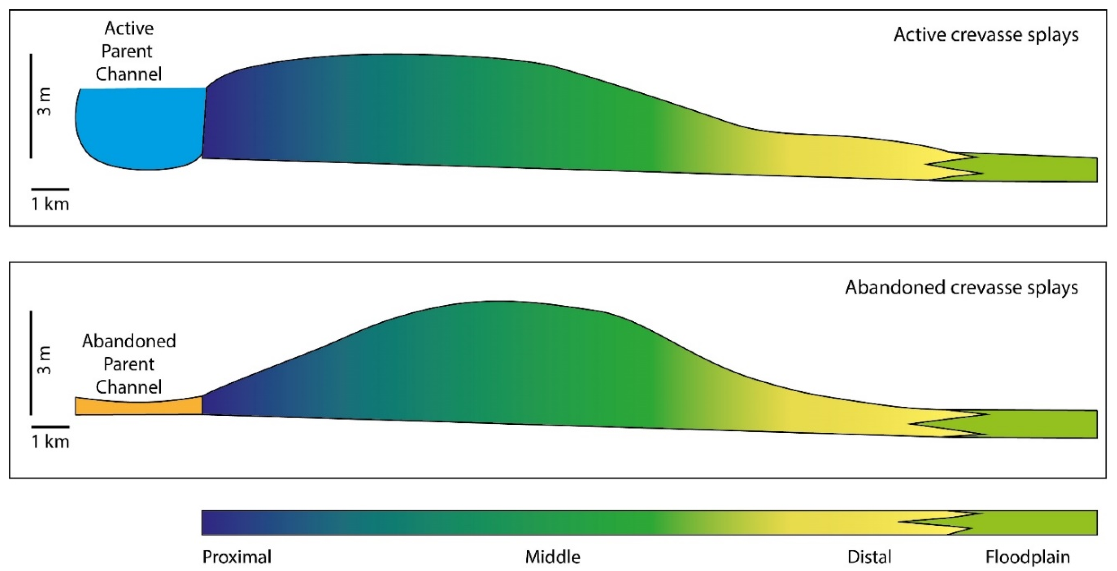
  • The spatial distribution of the crevasse deposit in the active landforms is generally controlled by the occurrence of vegetation, and the latter generally occurs in the proximal sector, favouring the transport of silt and clay up to the distal sector. The vegetation fixes the crevasse levees, favouring the channelized flow mainly in the proximal and middle sectors.
  • The maximum convexity of the along-dip altimetric profile shifts from the proximal-middle sectors of the active crevasse splays to the middle sector of the abandoned ones.
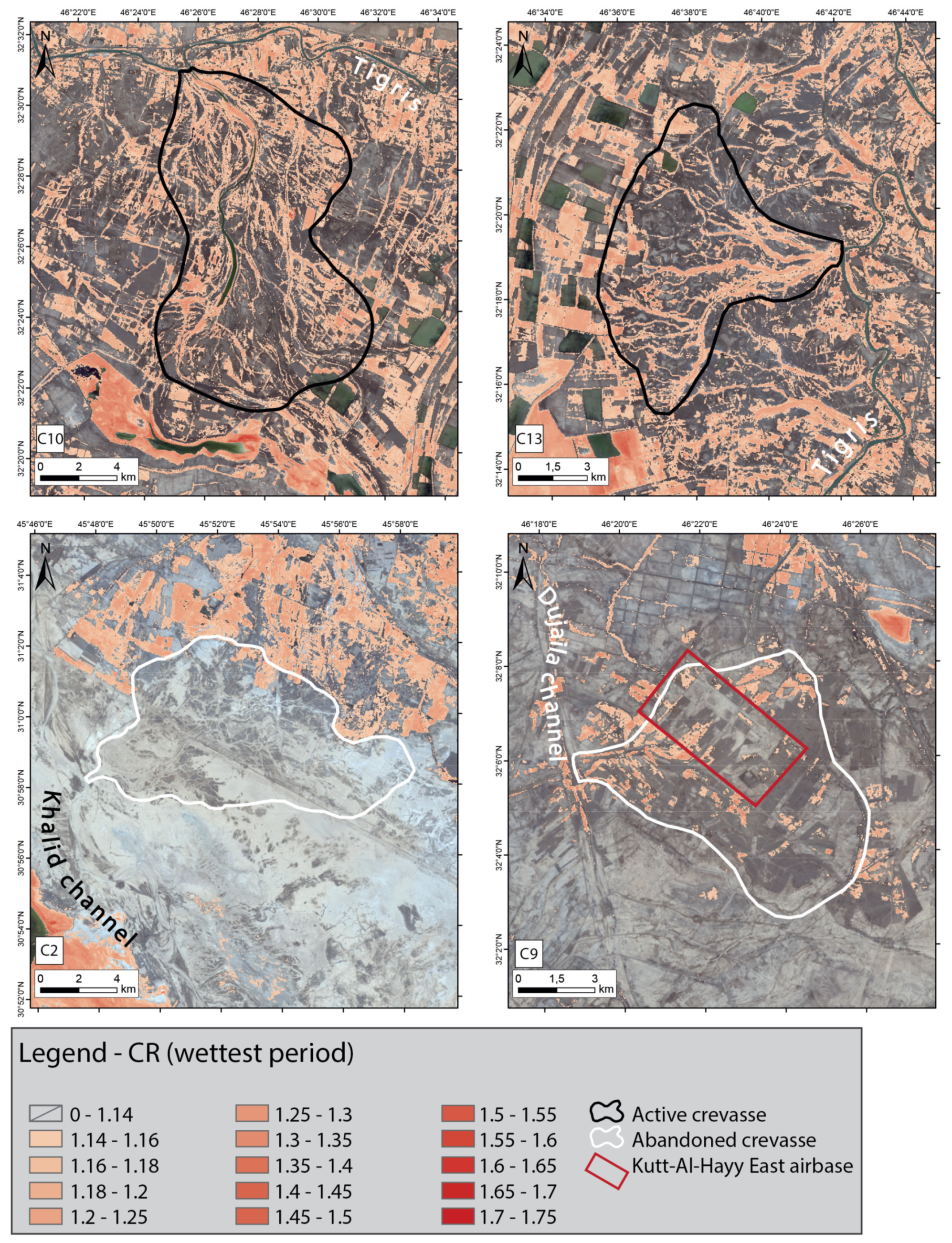
  • The CR can be used for a change detection of crevasse channels aimed at recognizing which step of a flood event we are observing, and thus for determining the state of activity of a crevasse splay as well as the NDVI.
  • The topographic analysis of the microrelief and the multispectral analysis are useful tools for discerning crevasse channels, levees, and deposits, improving their delimitation and mapping, especially for the active landforms.
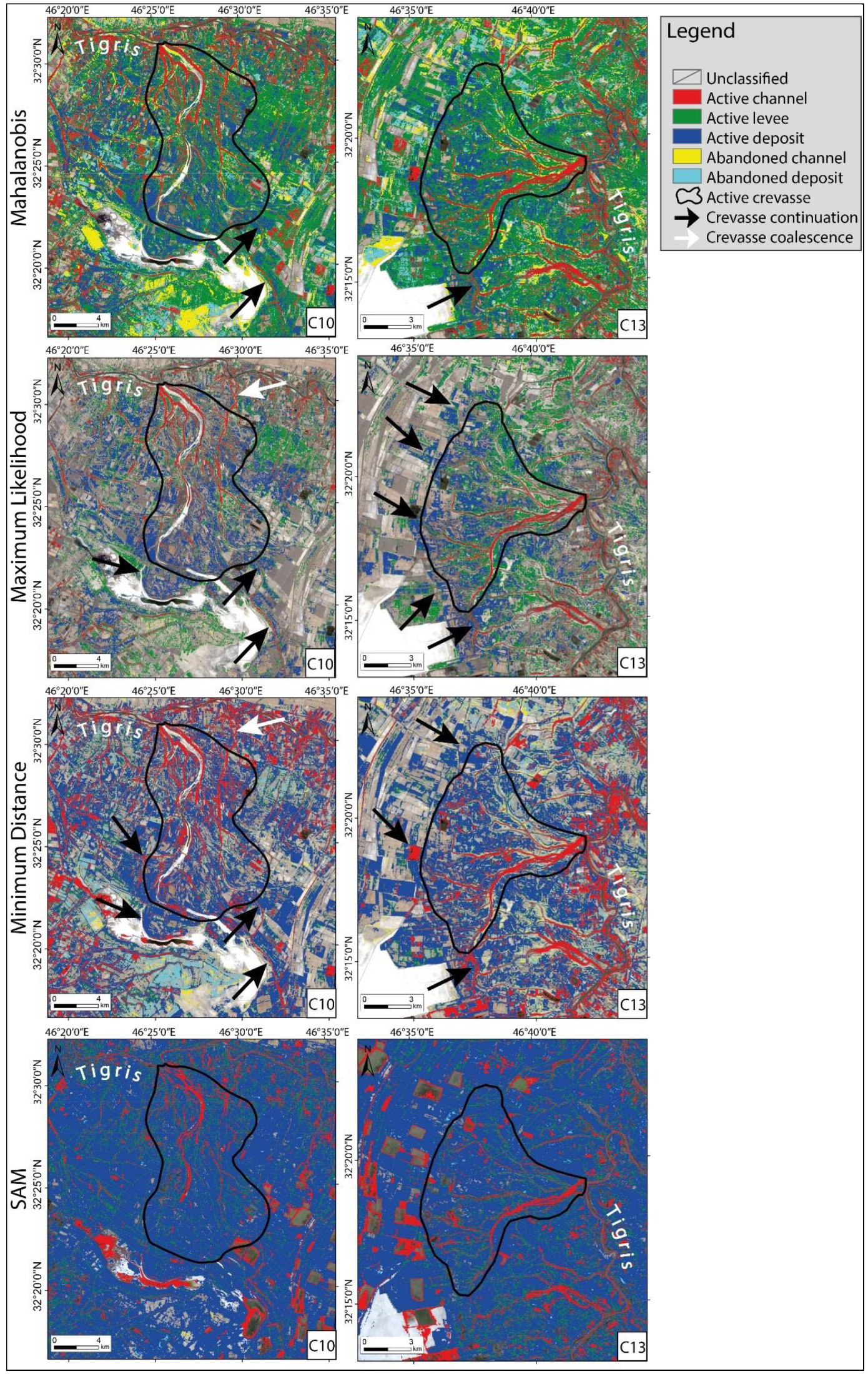
  • Maximum Likelihood proved to be the best classification method, whereas the SAM method proved unsuitable for detecting and mapping the crevasse features in the context of this work.
The results of this work can contribute to the evaluation of the risk associated along lowland areas to the formation and development of crevasse splays. Furthermore, in the specific study area, this work can contribute to the enhancement of knowledge concerning the Holocene waterscape dynamics that favoured the development of the first agricultural techniques and the development of the early human settlements.

Author Contributions

Conceptualization, G.I., F.T., and S.M.; methodology, G.I., F.T., S.M., and P.M.; software, G.I. and M.Z.; validation, D.P. and P.M.; investigation, G.I. and F.T.; data curation, G.I.; writing—original draft preparation, G.I.; writing—review and editing, F.T., S.M., D.P., and P.M.; visualization, G.I. and D.P.; supervision, F.T.; project administration, F.T. and D.N.; funding acquisition, D.N. All authors have read and agreed to the published version of the manuscript.

Funding

This research received no external funding.

Conflicts of Interest

The authors declare no conflict of interest.

References

  1. Allen, J.R.L. A review of the origin and characteristics of recent alluvial sediments. Sedimentology 1965, 5, 89–191. [Google Scholar] [CrossRef]
  2. Bridge, J.S.; Leeder, M.R. A simulation model of alluvial stratigraphy. Sedimentology 1979, 26, 617–644. [Google Scholar] [CrossRef]
  3. Jones, L.S.; Schumm, S.A. Causes of avulsion: An overview. In Fluvial Sedimentology VI; Smith, N.D., Rogers, J., Eds.; Blackwells: Oxford, UK, 1999; pp. 171–178. [Google Scholar]
  4. Bridge, J.S. Rivers and Floodplains: Forms, Processes, and Sedimentary Record; Blackwells: Oxford, UK, 2003. [Google Scholar]
  5. Slingerland, R.L.; Smith, N.D. River avulsions and their deposits. Annu. Rev. Earth Planet Sci. 2004, 32, 255–283. [Google Scholar] [CrossRef]
  6. Bridge, J.; Demicco, R. Earth Surface Processes, Landforms, and Sediment Deposits; Cambridge University Press: New York, NY, USA, 2008. [Google Scholar]
  7. Leeder, M. Sedimentology and Sedimentary Basins, 2nd ed.; Wiley-Blacvkwell: Oxford, UK, 2011. [Google Scholar]
  8. Bristow, C.; Skelly, R.; Ethridge, F. Crevasse splays from the rapidly aggrading, sand-bed, Niobrara River, Nebraska: Effect of base-level rise. Sedimentology 1999, 46, 1029–1048. [Google Scholar] [CrossRef]
  9. Smith, N.D.; Cross, T.A.; Dufficy, J.P.; Clough, S.R. Anatomy of an avulsion. Sedimentology 1989, 36, 1–23. [Google Scholar] [CrossRef]
  10. Smith, N.D.; Pérez-Arlucea, M. Fine-grained splay deposition in the avulsion belt of the lower Saskatchewan River, Canada. J. Sediment. Res. 1994, 64, 159–168. [Google Scholar]
  11. Buehler, H.A.; Weissmann, G.S.; Scuderi, L.A.; Hartley, A.J. Spatial and temporal evolution of an avulsion on the Taquari River distributive fluvial system from satellite image analysis. J. Sediment. Res. 2011, 81, 630–640. [Google Scholar] [CrossRef]
  12. Hajek, E.A.; Wolinsky, M.A. Simplified process modeling of river avulsion and alluvial architecture: Connecting models and field data. Sediment. Geol. 2012, 257–260, 1–30. [Google Scholar] [CrossRef]
  13. Bernal, C.; Christophoul, F.; Darrozes, J.; Laraque, A.; Bourrel, L.; Soula, J.C.; Guyot, J.L.; Baby, P. Crevassing and capture by floodplain drains as a cause of partial avulsion and anastomosis (lower Rio Pastaza, Peru). J. S. Am. Earth Sci. 2013, 44, 63–74. [Google Scholar] [CrossRef] [Green Version]
  14. Kleinhans, M.G.; Ferguson, R.I.; Lane, S.N.; Hardy, R.J. Splitting rivers at their seams: Bifurcations and avulsion. Earth Surf. Proc. Land. 2013, 38, 47–61. [Google Scholar] [CrossRef]
  15. Yuill, B.T.; Khadka, A.K.; Pereira, J.; Allison, M.A.; Meselhe, E.A. Morphodynamics of the erosional phase of crevasse-splay evolution and implications for river sediment diversion function. Geomorphology 2016, 259, 12–29. [Google Scholar] [CrossRef]
  16. Goudie, A.S. Encyclopedia of Geomorphology, 1st ed.; Routledge: London, UK, 2004; pp. 19–21, 381–384. ISBN 0–415–32737–7. [Google Scholar]
  17. Miall, A.D. The Geology of Fluvial Deposits, 4th ed.; Springer: Berlin/Heidelberg, Germany, 2006; pp. 172–176. ISBN 978-3-540-59186-3. [Google Scholar]
  18. Burns, C.; Mountney, N.P.; Hodgson, D.M.; Colombera, L. Anatomy and dimensions of fluvial crevasse-splay deposits: Examples from the Cretaceous Castlegate Sandstone and Neslen Formation, Utah, USA. Sediment. Geol. 2017, 351, 21–35. [Google Scholar] [CrossRef]
  19. Van Toorenenburg, K.A.; Donselaar, M.E.; Weltje, G.J. The life cycle of crevasse splays as a key mechanism in the aggradation of alluvial ridges and river avulsion. Earth Surf. Proc. Land. 2018, 43, 2409–2420. [Google Scholar] [CrossRef]
  20. Gulliford, A.R.; Flint, S.S.; Hodgson, D.M. Crevasse splay processes and deposits in an ancient distributive fluvial system: The lower Beaufort Group, South Africa. Sediment. Geol. 2017, 358, 1–18. [Google Scholar] [CrossRef]
  21. Millard, C.; Hajek, E.A.; Edmonds, D.A. Evaluating controls on crevasse-splay size: Implications for floodplain-basin filling. J. Sediment. Res. 2017, 87, 722–739. [Google Scholar] [CrossRef]
  22. Roberts, N. The Holocene: An Environmental History, 3rd ed.; Wiley-Blackweel: Oxford, UK, 2014. [Google Scholar]
  23. Walstra, J.; Heyvaert, V.M.A.; Verkinderen, P. Remote sensing for the study of fluvial landscapes in Lower Khuzestan, SW Iran. In Proceedings of the RSPSoc Annual Conference 2009, Leicester, UK, 8–11 September 2009. [Google Scholar]
  24. D’Arcy, M.; Masonc, P.J.; Roda-Boludab, D.C.; Whittakerc, A.C.; Lewisc, J.M.T.; Najorkad, J. Alluvial fan surface ages recorded by Landsat-8 imagery in Owens Valley, California. Remote Sens. Environ. 2018, 216, 401–414. [Google Scholar] [CrossRef] [Green Version]
  25. Borie, C.; Parcero-Obiῆa, C.; Kwon, Y.; Salazar, D.; Flores, C.; Olguìn, L.; Andrade, A. Beyond site detection: The role of satellite remote sensing in analysing archaeological problems. A case study in lithic resource procurement in the Atacama Desert, Northern Chile. Remote Sens. 2019, 11, 869. [Google Scholar] [CrossRef] [Green Version]
  26. Mihu-Pintilie, A.; Nicu, I.C. GIS-based landform classification of eneolithic archaeological sites in the plateau-plain transition zone (NE Romania): Habitation practices vs. flood hazard perception. Remote Sens. 2019, 11, 915. [Google Scholar] [CrossRef] [Green Version]
  27. Guyot, A.; Lennon, M.; Thomas, N.; Gueguen, S.; Petit, T.; Lorho, T.; Cassen, S.; Hubert-Moy, L. Airborne hyperspectral imaging for submerged archaeological mapping in shallow water environments. Remote Sens. 2019, 11, 2237. [Google Scholar] [CrossRef] [Green Version]
  28. Hill, A.C.; Laugier, E.J.; Casana, J. Archaeological remote sensing using multi-temporal, drone-acquired thermal and Near Infrared (NIR) Imagery: A case study at the Enfield Shaker Village, New Hampshire. Remote Sens. 2020, 12, 690. [Google Scholar] [CrossRef] [Green Version]
  29. Capolupo, A.; Monterisi, C.; Tarantino, E. Landsat Images Classification Algorithm (LICA) to automatically extract land cover information in Google Earth Engine environment. Remote Sens. 2020, 12, 1201. [Google Scholar] [CrossRef] [Green Version]
  30. Orengo, H.A.; Petrie, C.A. Large-scale, multi-temporal remote sensing of Palaeo-River Networks: A case study from Northwest India and its implications for the Indus civilisation. Remote Sens. 2017, 9, 735. [Google Scholar] [CrossRef] [Green Version]
  31. Morozova, G.S. A review of holocene avulsions of the Tigris and Euphrates rivers and possible effects on the evolution of civilizations in Lower Mesopotamia. Geoarchaeology 2005, 20, 401–423. [Google Scholar] [CrossRef]
  32. Wilkinson, T.J.; Rayne, L.; Jotheri, J. Hydraulic landscapes in Mesopotamia: The role of human niche construction. Water Hist. 2015, 7, 397–418. [Google Scholar] [CrossRef]
  33. Jotheri, J. Holocene Avulsion History of the Euphrates and Tigris Rivers in the Mesopotamian Floodplain. Ph.D. Thesis, Durham University, Durham, UK, June 2016. [Google Scholar]
  34. Yacoub, S.Y. Geomorphology of the Mesopotamia plain. Iraqi Bull. Geol. Min. 2011, 4, 7–32. [Google Scholar]
  35. Al-Ameri, I.D.S.; Briant, R.M. A late Holocene molluscan-based palaeoenvironmental reconstruction from southern Mesopotamia: Implications for the palaeogeographic evolution of the Arabo-Persian Gulf. J. Afr. Earth Sci. 2019, 152, 1–9. [Google Scholar] [CrossRef]
  36. Jotheri, J.; Allen, M.B.; Wilkinson, T.J. Holocene avulsions of the Euphrates river in the Najaf area of Western Mesopotamia: Impacts on human settlement patterns. Geoarchaeol. Int. J. 2016, 31, 175–193. [Google Scholar] [CrossRef]
  37. Engel, M.; Brückner, H. Holocene climate variability of Mesopotamia and its impact on the history of civilisation. EarthArXiv 2018. [Google Scholar] [CrossRef]
  38. Heyvaert, V.M.A.; Walstra, J. The role of long-term human impact on avulsion and fan development. Earth Surf. Proc. Land. 2016, 41, 2137–2152. [Google Scholar] [CrossRef]
  39. Garzanti, E.; Al-Juboury, A.I.; Zoleikhaei, Y.; Vermeesch, P.; Jotheri, J.; Akkoca, D.B.; Obaid, A.K.; Allen, M.B.; Andó, S.; Limonta, M.; et al. The Euphrates-Tigris-Karun river system: Provenance, recycling and dispersal of quartz-poor foreland-basin sediments in arid climate. Earth Sci. Rev. 2016, 162, 107–128. [Google Scholar] [CrossRef] [Green Version]
  40. Yacoub, S.Y.; Roffa, S.H.; Tawfiq, J.M. The Geology Al-Amara, Al-Nasiriya, Al-Basrah Area; International Report no. 1386; GEOSURV: Baghdad, Iraq, 1985. [Google Scholar]
  41. Aqrawi, A.A.M.; Evans, G. Sedimentation in the lake and marshes (Ahwar) of the Tigris and Euphrates delta. Sedimentology 1994, 41, 755–776. [Google Scholar] [CrossRef]
  42. Yacoub, S.Y. Stratigraphy of the Mesopotamia Plain. Iraqi Bull. Geol. Min. 2011, 4, 47–82. [Google Scholar]
  43. Lees, G.M.; Falcon, N.L. The geographical history of the Mesopotamian plains. Geogr. J. 1952, 118, 24–39. [Google Scholar] [CrossRef]
  44. Lambeck, K. Shoreline reconstructions for the Persian Gulf since the last glacial maximum. Earth Planet. Sci. Lett. 1996, 142, 43–57. [Google Scholar] [CrossRef]
  45. Aqrawi, A.A.M. Stratigraphic signatures of climatic change during the Holocene evolution of the Tigris–Euphrates delta, lower Mesopotamia. Glob. Planet. Chang. 2001, 28, 267–283. [Google Scholar] [CrossRef]
  46. Kennett, D.J.; Kennett, J.P. Early state formation in Southern Mesopotamia: Sea levels, shorelines, and climate change. J. Isl. Coast. Archaeol. 2006, 1, 67–69. [Google Scholar] [CrossRef]
  47. Milli, S.; Forti, L. Geology and palaeoenvironment of Nasiriyah area/southern Mesopotamia. In Abu Tbeirah Excavations I. Area 1, 1st ed.; Romano, L., D’Agostino, F., Eds.; Sapienza Università Editrice: Roma, Italy, 2019; pp. 19–33. ISBN 978-88-9377-108-5. [Google Scholar]
  48. Sissakian, V.K.; Adamo, N.; Al-Ansari, N.; Abdullah, M.; Laue, J. Sea level changes in the Mesopotamian Plain and limits of the Arabian Gulf: A critical review. J. Earth Sci. Geotech. Eng. 2020, 10, 87–110. [Google Scholar]
  49. Bogemans, F.; Janssens, R.; Baeteman, C. Depositional evolution of the Lower Khuzestan plain (SW Iran) since the end of the Late Pleistocene. Quat. Sci. Rev. 2017, 171, 154–165. [Google Scholar] [CrossRef]
  50. Bogemans, F.; Boudin, M.; Janssens, R.; Baeteman, C. New data on the sedimentary processes and timing of the initial inundation of Lower Khuzestan (SW Iran) by the Persian Gulf. Holocene 2017, 27, 613–620. [Google Scholar] [CrossRef]
  51. Pournelle, J.R. Marshland of Cities: Deltaic Landscapes and the Evolution of Early Mesopotamian Civilization. Ph.D. Thesis, Univeristy of California, San Diego, CA, USA, 2003; p. 314. [Google Scholar]
  52. Pournelle, J.R. Physical geography. In The Sumerian World; Crawford, H., Ed.; Routledge Taylor & Francis Group: London, UK; New York, NY, USA, 2013; pp. 13–32. [Google Scholar]
  53. Jotheri, J.; Altaweel, M.; Tuji, A.; Anma, R.; Pennington, B.; Rost, S.; Watanabe, C. Holocene fluvial and anthropogenic processes in the region of Uruk in southern Mesopotamia. Quat. Int. 2018, 483, 57–69. [Google Scholar] [CrossRef]
  54. Heyvaert, V.M.A.; Walstra, J.; Verkinderen, P.; Weerts, H.J.T.; Ooghe, B. The role of human interference on the channel shifting of the Karkheh River in the Lower Khuzestan plain (Mesopotamia, SW Iran). Quat. Int. 2012, 251, 52–63. [Google Scholar] [CrossRef]
  55. Macklin, M.G.; Lewin, J. The rivers of civilization. Quat. Sci. Rev. 2015, 114, 228–244. [Google Scholar] [CrossRef]
  56. Jotheri, J. Recognition criteria for canals and rivers in the Mesopotamian floodplain. In Water Societies and Technologies from the Past and Present, 1st ed.; Zhuang, Y., Altaweel, M., Eds.; UCL Press: London, UK, 2018; pp. 111–126. ISBN 978-1-911576-69-3. [Google Scholar]
  57. Waterman, R. ArcGIS Blog. Available online: https://www.esri.com/arcgis-blog/products/arcgis-living-atlas/imagery/whats-new-in-world-imagery-basemap-july-2017-through-june-2018/ (accessed on 4 April 2020).
  58. World Imagery. Available online: https://www.arcgis.com/home/item.html?id=10df2279f9684e4a9f6a7f08febac2a9 (accessed on 4 April 2020).
  59. Mudd, S.M. Topographic data from satellites. In Remote Sensing of Geomorphology; Developments in Earth Surface Processes; Tarolli, P., Mudd, S.M., Eds.; Elsevier: Amsterdam, The Netherlands, 2020; Volume 23, pp. 91–128. [Google Scholar]
  60. Santillan, J.R.; Makinano-Santillan, M.; Makinano, R.M. Vertical accuracy assessment of ALOS World 3D-30M Digital Elevation Model over northeastern Mindanao, Philippines. In Proceedings of the 2016 IEEE International Geoscience and Remote Sensing Symposium (IGARSS), Beijing, China, 10–15 July 2016; pp. 5374–5377. [Google Scholar]
  61. Tachikawa, T.; Kaku, M.; Iwasaki, A.; Gesch, D.; Oimoen, M.; Zhang, Z.; Danielson, J.; Krieger, T.; Curtis, B.; Haase, J.; et al. ASTER Global Digital Elevation Model Version 2—Summary of Validation Results. Available online: https://ssl.jspacesystems.or.jp/ersdac/GDEM/ver2Validation/Summary_GDEM2_validation_report_final.pdf (accessed on 19 April 2020).
  62. Kahle, A.B.; Shumate, M.S.; Nash, D.B. Active airborne infrared laser system for identification of surface rock and minerals. Geophys. Res. Lett. 1984, 11, 1149–1152. [Google Scholar] [CrossRef]
  63. Gillespie, A.R. Spectral mixture analysis of multispectral thermal infrared images. Remote Sens. Environ. 1992, 42, 137–145. [Google Scholar] [CrossRef]
  64. Bull, W.B. Geomorphic Responses to Climatic Change; Oxford University Press: New York, NY, USA, 1991; ISBN 978-1932846218. [Google Scholar]
  65. Roy, D.P.; Wulder, M.A.; Loveland, T.R.; Woodcock, E.; Allen, R.G.; Anderson, M.C.; Helder, D.; Irons, J.R.; Johnson, D.M.; Kennedy, R.; et al. Landsat-8: Science and product vision for terrestrial global change research. Remote Sens. Environ. 2014, 145, 154–172. [Google Scholar] [CrossRef] [Green Version]
  66. Sekandari, M.; Masoumi, I.; Pour, A.B.; Muslim, A.M.; Rahmani, O.; Hashim, M.; Zoheir, B.; Pradhan, B.; Misra, A.; Aminpour, S.M. Application of Landsat-8, Sentinel-2, ASTER and WorldView-3 spectral imagery for exploration of carbonate-hosted Pb-Zn deposits in the CENTRAL IRANIAN TERRANE (CIT). Remote Sens. 2020, 12, 1239. [Google Scholar] [CrossRef] [Green Version]
  67. USGS Landsat Missions. Available online: https://www.usgs.gov/land-resources/nli/landsat/landsat-8?qt-science_support_page_related_con=0#qt-science_support_page_related_con (accessed on 20 May 2020).
  68. Dawson, H.F. Water flow and the vegetation of running waters. In Vegetation of Inland Waters, 1st ed.; Symoens, J.J., Ed.; Kluwer Academic Publishers: Dordrecht, The Netherlands, 1988; Volume 15-1, pp. 283–309. ISBN 978-94-010-7887-0. [Google Scholar]
  69. Hiatt, M.; Passalacqua, P. What controls the transition from confined to unconfined flow? Analysis of hydraulics in a coastal river delta. J. Hydraul. Eng. 2017, 143. [Google Scholar] [CrossRef]
  70. L3 Harris Geospatial. Classification. Available online: https://www.harrisgeospatial.com/docs/Classification.html#ClassSupervised (accessed on 19 April 2020).
  71. Liu, J.G.; Mason, P.J. Image classification. In Essential Image Processing and GIS for Remote Sensing, 1st ed.; Wiley-Blackwell: Oxford, UK, 2009; pp. 91–103. ISBN 978-0-470-51032-2. [Google Scholar]
  72. Pontius, R.G., Jr.; Millones, M. Death to Kappa: Birth of quantity disagreement and allocation disagreement for accuracy assessment. Int. J. Remote Sens. 2011, 32, 4407–4429. [Google Scholar] [CrossRef]
  73. L3 Harris Geospatial. Calculate Confusion Matrices. Available online: https://www.harrisgeospatial.com/docs/CalculatingConfusionMatrices.html (accessed on 2 March 2020).
  74. Humboldt State University. Accuracy Metrics. Available online: http://gis.humboldt.edu/OLM/Courses/GSP_216_Online/lesson6-2/metrics.html (accessed on 3 March 2020).
  75. Banko, G. A Review of Assessing the Accuracy of Classifications of Remotely Sensed Data and of Methods Including Remote Sensing Data in Forest Inventory; Interim Report IR-98-081; University of Agricultural Sciences: Wien, Austria, 1998. [Google Scholar]
  76. Jotheri, J.; de Gruchy, M.W.; Almaliki, R.; Feadha, M. Remote sensing the archaeological traces of boat movement in the marshes of Southern Mesopotamia. Remote Sens. 2019, 11, 2474. [Google Scholar] [CrossRef] [Green Version]
Figure 1. Satellite nadiral view of the study area from TerraColor satellite imagery and distribution of the crevasse splays in the investigated area. Black rectangles indicate the floodplain sectors where the crevasse splays reported and discussed in this work. (A) active crevasse splays along the present Tigris fluvial system (C10 and C13); (B) abandoned crevasse splay along an ancient watercourse (C9); (C) abandoned crevasse splay along an ancient watercourse belonging to the Euphrates fluvial system (C2).
Remotesensing 12 02243 g001
Figure 2. Conceptual sketch of a typica fan-shaped crevasse splays due to a levee break at the external zone of a river belt. The along-dip crevasse sub-division adopted in this work is reported. Direction and terminology for the altimetric profiles elaborated in this work is also shown. Keys: XX’: along-dip direction; YY’ cross direction.
Remotesensing 12 02243 g002
Figure 3. The tiles of Landsat 8 available for the LMP. The tiles are identified by their Path-Row code in the table, specifying the acquisition date for the wettest and driest period.
Remotesensing 12 02243 g003
Figure 4. Example for producer and user accuracy (sensu Banko 1998) for a typical landforms association of a crevasse splay.
Remotesensing 12 02243 g004
Figure 5. The adopted methodological scheme (workflow and software) for the analyses conducted in this research.
Remotesensing 12 02243 g005
Figure 6. Example of active (C10, C13) and abandoned (C2, C9) crevasse splays recognized in the area. The traces of altimetric profiles shown in Figure 8 and Figure 9 are reported: AA’: along-dip profiles, BB’: cross-direction profiles of the proximal sector, CC’: cross-direction profiles of the middle sector, DD’: cross-direction profiles of the distal sector.
Remotesensing 12 02243 g006
Figure 7. Example of the differences between the altimetric configuration of crevasse C10 as visualized using the AW3D30 (A) and GDEM2 (B) datasets.
Remotesensing 12 02243 g007
Figure 8. Altimetric profiles based on elevation data of both AW3D30 (blue line) and GDEM2 (red line) datasets. Moving averaged values range from 10 up to 20 m. Location of the profile traces are reported in Figure 6. (A) Altimetric profiles for the crevasse C10; (B) Altimetric profiles for the crevasse C13.
Remotesensing 12 02243 g008
Figure 9. Altimetric profiles based on elevation data of both AW3D30 (blue line) and GDEM2 (red line) datasets. Moving averaged values range from 8 up to 20 m. Location of the profile traces are reported in Figure 5. (A) Altimetric profiles for the crevasse C2; (B) Altimetric profiles for the crevasse C9.
Remotesensing 12 02243 g009
Figure 10. Spatial distribution of NDVI, during the wettest period, for the active (C10, C13) and the abandoned (C2, C9) crevasse splays.
Remotesensing 12 02243 g010
Figure 11. Spatial distribution of the CR, during the wettest period, for the active (C10, C13) and the abandoned (C2, C9) crevasse splays.
Remotesensing 12 02243 g011
Figure 12. Classified active crevasse splay (C10, C13) using four classification methods. For the Mahalanobis and Minimum Distance the wettest period is shown, while for the Maximum Likelihood and SAM is the driest period.
Remotesensing 12 02243 g012
Figure 13. Classified abandoned crevasse splay (C2, C9) using four classification methods. For the Mahalanobis and Minimum Distance the wettest period is shown, while for the Maximum Likelihood and SAM is the driest period.
Remotesensing 12 02243 g013
Figure 14. The re-mapping of active (C10 and C13) and abandoned (C2 and C9) crevasses for highlighting the hierarchy of the single flood event.
Remotesensing 12 02243 g014
Figure 15. Along-dip conceptual altimetric profiles of typical active and abandoned crevasse splays as inferred from this research. Crevasse splay sections terminology according to Figure 1.
Remotesensing 12 02243 g015
Table 1. The most accurate thresholds for each classification method.
Driest Period
Active ChannelActive LeveeActive DepositAbandoned ChannelAbandoned Deposit
Mahalanobis
(Maximum distance error)
30002000200020002000
Maximum Likelihood
(Probability threshold)
0.300.700.300.300.30
Minimum distance
(Standard deviation from mean)
4.001.503.001.503.00
SAM
(Maximum spectral angle)
0.100.040.050.0080.008
Wettest period
Mahalanobis
(Maximum distance error)
30001500150010001000
Maximum Likelihood
(Probability threshold)
0.200.600.400.600.30
Minimum Distance
(Standard deviation from mean)
3.002.002.001.501.30
SAM
(Maximum spectral angle)
0.100.030.030.010.015
Table 2. Accuracy of each ROIs derived from the different classification methods applied in this work.
Driest PeriodWettest Period
OA (%)KOA (%)K
Mahalanobis66.00260.514867.94020.5755
Maximum Likelihood69.18010.563667.75340.5925
Minimum Distance62.01840.460758.44800.4841
SAM61.27760.367663.94970.4655
Driest PeriodWettest Period
PA (%)UA (%)PA (%)UA (%)
MahalanobisActive channel69.1890.8876.7370.07
Active levee54.2417.4924.4235.15
Active deposit67.5598.0568.2994.92
Abandoned channel54.2273.8346.1768.20
Abandoned deposit72.2657.3184.9273.18
Maximum LikelihoodActive channel79.9299.7479.6599.09
Active levee23.7346.6737.6860.47
Active deposit71.1798.9766.4296.71
Abandoned channel63.9196.2452.6388.71
Abandoned deposit73.2978.4974.4098.85
Minimum DistanceActive channel70.5683.1588.5679.29
Active levee34.7514.4947.7929.75
Active deposit66.4696.4645.8091.24
Abandoned channel28.9187.2966.5189.39
Abandoned deposit69.3676.4846.4295.96
SAMActive channel71.8258.4875.0077.37
Active levee27.9719.8811.3741.22
Active deposit76.0079.7684.8264.04
Abandoned channel7.5024.2454.5579.17
Abandoned deposit25.0526.0219.0997.78

