Article

Investigating Live Fuel Moisture Content Estimation in Fire-Prone Shrubland from Remote Sensing Using Empirical Modelling and RTM Simulations

1
AGRESTA S. Coop., calle Duque de Fernán Núñez 2, 28012 Madrid, Spain
2
Australian National University, Fenner School of Environment & Society, Forestry Building (48), Linnaeus Way, ACTON ACT 2601, Canberra, Australia
3
Australian National University, Research School of Aerospace, Mechanical and Environmental Engineering 2601, Canberra, Australia
4
Bushfire and Natural Hazards CRC, Melbourne, 3002 Victoria, Australia
5
INIA, Forest Research Centre, Department of Silviculture and Forest Management, Forest fire laboratory. Crta. A Coruña Km 7.5, 28040 Madrid, Spain
6
iuFOR, University Institute for Sustainable Forest Management, uVA-INIA, 34004 Palencia, Spain
*
Author to whom correspondence should be addressed.
Remote Sens. 2020, 12(14), 2251; https://0-doi-org.brum.beds.ac.uk/10.3390/rs12142251
Submission received: 6 June 2020 / Revised: 11 July 2020 / Accepted: 12 July 2020 / Published: 14 July 2020
(This article belongs to the Collection Sentinel-2: Science and Applications)

Abstract

:
Previous research has demonstrated that remote sensing can provide spectral information related to vegetation moisture variations essential for estimating live fuel moisture content (LFMC), but accuracy and timeliness still present challenges to using this information operationally. Consequently, many regional administrations are investing important resources in field campaigns for LFMC monitoring, often focusing on indicator species to reduce sampling time and costs. This paper compares different remote sensing approaches to provide LFMC prediction of Cistus ladanifer, a fire-prone shrub species commonly found in Mediterranean areas and used by fire management services as an indicator species for wildfire risk assessment. Spectral indices (SI) were derived from satellite imagery of different spectral, spatial, and temporal resolution, including Sentinel-2 and two different reflectance products of the Moderate Resolution Imaging Spectrometer (MODIS); MCD43A4 and MOD09GA. The SI were used to calibrate empirical models for LFMC estimation using on ground field LFMC measurements from a monospecific shrubland area located in Madrid (Spain). The empirical models were fitted with different statistical methods: simple (LR) and multiple linear regression (MLR), non-linear regression (NLR), and general additive models with splines (GAMs). MCD43A4 images were also used to estimate LFMC from the inversion of radiative transfer models (RTM). Empirical model predictions and RTM simulations of LFMC were validated and compared using an independent sample of LFMC values observed in the field. Empirical models derived from MODIS products and Sentinel-2 data showed R2 between estimated and observed LFMC from 0.72 to 0.75 and mean absolute errors ranging from 11% to 13%. GAMs outperformed regression methods in model calibration, but NLR had better results in model validation. LFMC derived from RTM simulations had a weaker correlation with field data (R2 = 0.49) than the best empirical model fitted with MCD43A4 images (R2 = 0.75). R2 between observations and LFMC derived from RTM ranged from 0.56 to 0.85 when the validation was performed for each year independently. However, these values were still lower than the equivalent statistics using the empirical models (R2 from 0.65 to 0.94) and the mean absolute errors per year for RTM were still high (ranging from 25% to 38%) compared to the empirical model (ranging 7% to 15%). Our results showed that spectral information derived from Sentinel-2 and different MODIS products provide valuable information for LFMC estimation in C. ladanifer shrubland. However, both empirical and RTM approaches tended to overestimate the lowest LFMC values, and therefore further work is needed to improve predictions, especially below the critical LFMC threshold used by fire management services to indicate higher flammability (<80%). Although lower extreme LFMC values are still difficult to estimate, the proposed empirical models may be useful to identify when the critical threshold for high fire risk has been reached with reasonable accuracy. This study demonstrates that remote sensing data is a promising source of information to derive reliable and cost-effective LFMC estimation models that can be used in operational wildfire risk systems.

Graphical Abstract

1. Introduction

Wildfire activity is highly influenced by fuel characteristics, especially vegetation moisture dynamics [1,2]. Live fuel moisture content (LFMC) has been proven to be a major driver of vegetation flammability and fire behavior as it determines both the ability of ignition and the spread rate of flames [3,4,5]. Due to the dampening effect of water content in plant tissues, vegetation may act as a heat source or sink in a wildfire depending on LFMC level, thus conditioning fire front progression and transition from surface to crown fires [6,7].
Many regions around the world are suffering more frequent extreme weather conditions and an extension of the fire season along the year, with even worse scenarios projected in the future [8,9]. In Southern Europe, global change has also led to a shift in fire regimes from fuel-limited to drought-driven due to rural abandonment that favors fuel build-up in unmanaged landscapes [10,11]. Current wildfire 3D models and simulation tools are useful for predicting potential fire behavior and severity at the landscape level, but they require detailed and spatially-explicit fuel characteristics, including LFMC, as key input parameters [12,13,14,15]. So, there is an increasing need for reliable and updated spatial and temporal estimations of LFMC to improve fire danger rating systems and the emergency response [16].
Despite its relevance, the estimation of LFMC variation is still uncertain because of the complex interaction between weather, plants, and soil characteristics [17]. Research institutions and management services in many countries are investing an important amount of resources on field-based vegetation monitoring to understand LFMC dynamics and support operational fire management activities for wildfire prevention and suppression planning [17,18]. Field sampling is expensive and time-consuming, implying also a delay time until moisture data are available, hence fire managers often focus on only collecting data from indicator species that are relevant for wildfire risk assessment.
Remote sensing is the only efficient alternative that can provide systematic and accurate vegetation monitoring on a large scale. Previous research highlights the ability of satellite imagery for LFMC estimation at different spatial and temporal resolutions [19]. Among optical sensors, the Moderate Resolution Imaging Spectrometer (MODIS) is commonly used to this end due to its adequate temporal and spectral resolution. Many authors proposed empirical models to estimate LFMC from several spectral indices derived from MODIS data [20,21,22,23]. However, MODIS provides spectral information at a coarse spatial resolution (500 m in the near to short wave infrared, NIR to SWIR), which may limit its use in areas with heterogeneous vegetation or strong topographic effects that determine differences in moisture conditions. Sentinel-2 is a new generation of sensors with similar spectral information to MODIS and extra red-edge bands but with a higher spatial resolution (ranging from 10 m to 60 m) which provides an opportunity to potentially improve LFMC estimations and the applications of the final products for more detailed wildfire management. Nevertheless, to date, there are still very few studies testing Sentinel-2 imagery for LFMC estimation [24], and no study has carried out a comprehensive analysis of Sentinel-2 capability in comparison to other commonly-used sensors. Some authors have assessed the potential of microwave remote sensing for LFMC estimation, obtaining moderate results compared to optical indices derived from MODIS [25,26]. Recently, Wang et al. [27] tested the performance of synthetic aperture radar (SAR) from Sentinel-1A for LFMC retrieval, obtaining better results compared to Landsat data.
In addition to the empirical modeling of LFMC, some authors proposed the use of radiative transfer models (RTM) to retrieve LFMC from optical sensors. RTM is a more complex method based on physical approaches from simulations that can provide robust LFMC estimations independent of site specificities [19,28,29,30,31]. Yebra et al. [29] compared the performance of empirical and statistical models based on RTM from MODIS images for LFMC estimation, reporting good results for Mediterranean grassland and shrubland in central Spain. However, these authors used MODIS data from an 8-day composite product that may not be ideal for LFMC retrieval with operational purposes. Shu et al. [24] combined Sentinel-2A data and coupled RTMs to retrieve LFMC in different types of vegetation, including grassland, shrubland, and forest ecosystems from USA, South Africa, Australia, and France, with promising preliminary results in terms of correlation (R2 = 0.64), but still obtaining low accuracies (RMSE = 47%).
Research on LFMC estimation from satellite imagery to date has been mainly focused on composite products that are useful to study vegetation dynamics, but there is a lack of information regarding the ability of near-real-time remote sensing data for LFMC retrieval. Hence, accurate LFMC estimation is still a challenge at an operational level, either through empirical modeling or RTM approaches, which is a requirement for its integration into efficient fire pre-alert systems.
The aims of the present study are: (i) to assess the potential of satellite images of different spectral, spatial and temporal resolutions collected by Sentinel-2 and MODIS to estimate LFMC, including operational and non-operational products, and (ii) to compare the performances of empirical models and RTM simulations based on the same MODIS product, assessing model accuracy within the framework of previous results. We focused on Cistus ladanifer L., a fire-prone species commonly found in Mediterranean shrubland areas. C. ladanifer is used by fire management services as an indicator species for wildfire risk assessment. To our knowledge, this is the first study carrying out a comprehensive analysis of Sentinel-2 capability in comparison to other sensors and retrieval algorithms.

2. Methods

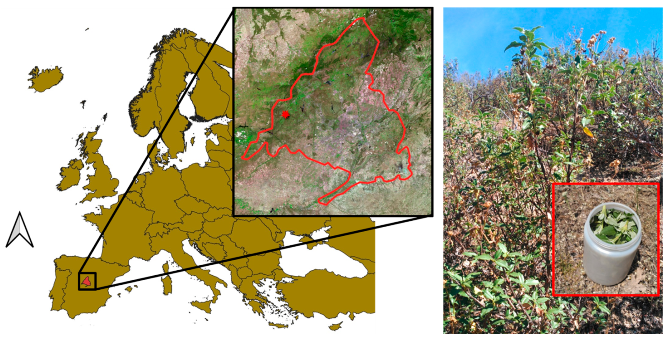
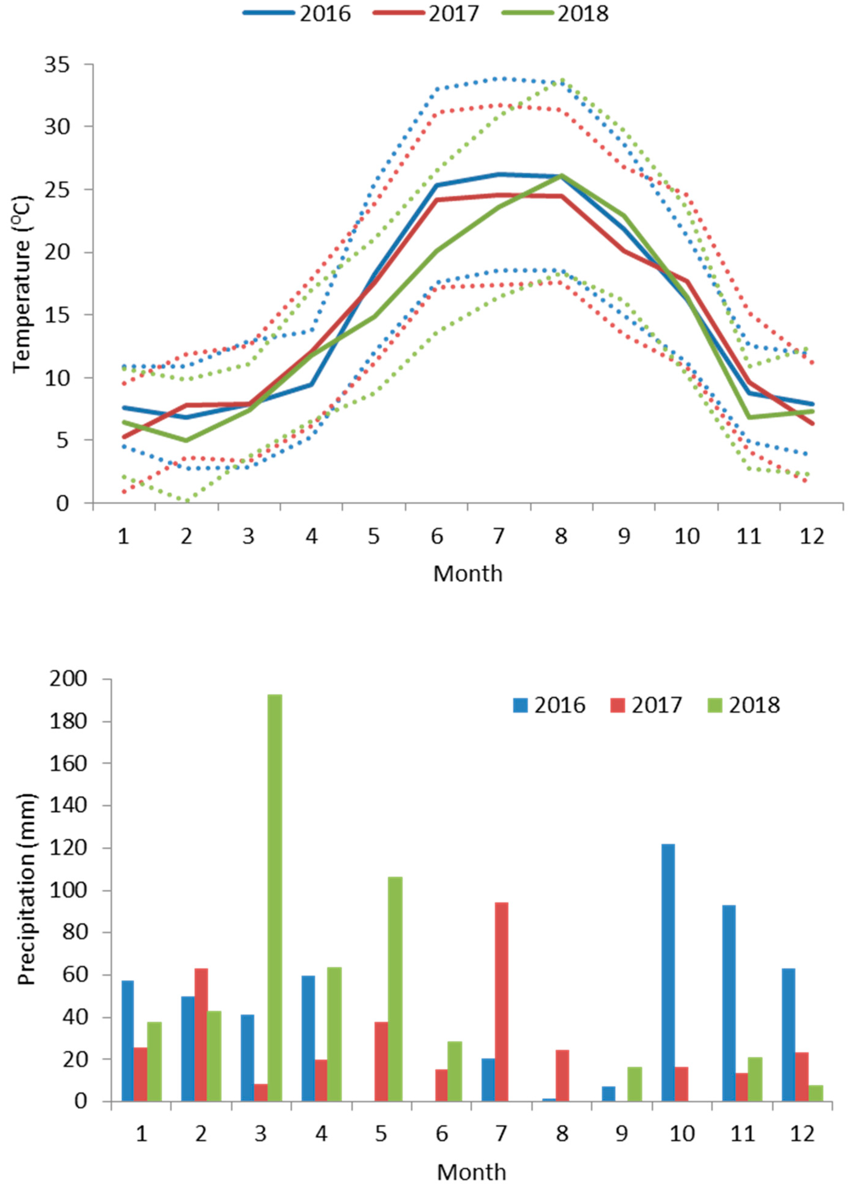
2.1. Study Area and Reference Data

The study area is a 45 ha monospecific shrubland located in the Madrid region, Central Spain (40°30′ N, 4°12′ W) (Figure 1). Vegetation is dominated by C. ladanifer, a shrub species that has been identified by Spanish regional fire management services as a fire risk indicator species due to the high seasonal variability and the low minimum moisture values reached during the fire season. The climate is typically Mediterranean, with hot dry summers and rainfalls occurring mainly during spring and autumn. The average minimum and maximum temperatures are 1 °C in winter and 31 °C in summer, respectively, and mean annual precipitation is 450 mm.
Samples of C. ladanifer live fine fuels, including leaves and terminal twigs (Figure 1), were systematically collected in the study area according to a field protocol defined by the Forest Fire Laboratory of the Spanish National Institute for Agricultural and Food Research and Technology (INIA). Random linear transects were established in order to avoid re-sampling of the same plants throughout the study period. Between 50–100 g of fine fuel, i.e., twigs and leaves lesser than 6 mm according to Fosberg and Deeming [32], were extracted using a manual saw on at least five different plants along the selected transect. Samples were collected at 12:00 AM on a sunny hill facing southeast, were introduced in a hermetic plastic recipient, and were transported to the laboratory before 3:00 PM to avoid potential humidity loss. Sampling frequency varied along the year, starting in spring 2016, with an increased frequency from up to three days during the summer, weekly during spring and autumn, and biweekly in winter. Fresh samples were weighed daily in a laboratory, and then oven-dried at 100 °C for 24 h and weighed dry for moisture content estimation. LFMC was calculated as the percentage of water content of vegetation on a dry-weight basis.
A total of 143 field samples were available for the study area. Reference data were carefully selected in order to exclude any sample with potential LFMC anomaly detected due to incorrect field sampling (e.g., dead leaves, flowers or fruits included), previous rainfall, or loss of moisture prior to laboratory processing.

2.2. Remote Sensing Data

2.2.1. Image Selection and Preprocessing

Spectral information derived from two types of satellite sensors was used: the Moderate Resolution Imaging Spectroradiometer (MODIS) and the Sentinel-2 Multi-Spectral Instrument (MSI). MODIS provides daily images with a coarse spatial resolution (250 m, 500 m or 1000 m). Sentinel-2 satellites provide images at a finer spatial resolution, revisiting the same portion of the earth at least every 5 days with the two satellites (2A and 2B) available. The high-resolution optical sensor (MSI) included in Sentinel-2 satellites operates in 13 bands between the visible and the SWIR. The spatial resolution is 10 m for visible and NIR bands, 20 m for red-edge and SWIR bands, and 60 m for atmospheric bands.
Two standard products of MODIS were selected: (i) MCD43A4, a 16-day composite that combines images from Terra an Aqua satellites, which is daily available but with a timelag until the 16-day composite period is completed, and (ii) MOD09GA, a non-composite daily product provided by Terra satellite that has the drawback of depending on cloud-free image availability. We choose MOD09GA over other similar MODIS products provided by Aqua satellite (e.g., MYD09GA) because image acquisition time was closer to field data collection time (MODIS Terra is before noon, whereas MODIS Aqua is later in the afternoon). Both MODIS products corresponded to atmospherically-corrected surface reflectance, and MCD43A4 also include bidirectional reflectance distribution function (BRDF) correction. The images were downloaded from the NASA Land Processess Distributed Active Archive Center (LP DAAC, https://lpdaac.usgs.gov/).
Sentinel-2 products are non-composite images. Sen2Cor software [33] from the European Space Agency (ESA) was used to convert the original bands (Level 1C images) from the top of the atmosphere (TOA) to corrected reflectances at the bottom of the atmosphere (BOA).

2.2.2. Spectral Indices

A set of spectral indices (SI) derived from MODIS images were calculated at 500 m resolution (Table 1). The same MODIS indices were calculated for Sentinel-2 images at a 20 m pixel resolution, with the exception of NDWI that cannot be computed due to the spectral resolution of Sentinel-2 (lack of an equivalent formulation for the two NIR bands in MODIS). Instead, an additional index for the red-edge (NDI45) was tested for Sentinel-2 images (Table 1).
To compare image reflectance and LFMC field measurements, the extraction of pixel data for the calculation of SI values was performed accounting for the different spatial resolutions of each sensor. In the case of MODIS images (500 m), different pixels covered the study area but were not completely included. Therefore, SI values calculated from MODIS products corresponded to the weighted mean of pixel values according to the portion of each pixel surface overlapping the study area. For Sentinel-2 (20 m), SI values were the mean values of the pixels completely included inside the study area.

2.3. Empirical Methods

Empirical methods were used to estimate LFMC from SI derived from the three selected products collected by MODIS and Sentinel-2 satellite sensors. The temporal variability of LFMC observed in the field was assessed and compared with the temporal profiles of each SI. In addition, specific Pearson correlation matrices between LFMC and the SI were obtained for each type of sensor and MODIS product (Table 1).
The statistical methods assessed for empirical modeling included simple linear regression (LR), multivariate linear regression (MLR), non-linear regression (NLR), and general additive models with splines (GAMs). LFMC distribution in all datasets was tested for normality using the Shapiro-Wilk test before regression analysis. Collinearity among potential predictors was checked using the variance inflation factor (VIF), rejecting models with VIF > 5 for any variable included.
Models were fitted with 67% of the samples (calibration dataset), and then applied to the rest of the field measured LFMC (33% of samples) to get an independent validation. We systematically selected one out of three observations for the validation dataset for each year, and checked that the whole range of LFMC values was represented in both the calibration and validation datasets.
Model performance was assessed with the coefficient of determination (adjusted value of R2 to compare goodness-of-fit between models with a different number of input variables), mean absolute error (MAE), and root mean square error (RMSE). Statistical analyses were performed in R Software [42].

2.4. Radiative Transfer Model (RTM) Simulations

A radiative transfer model (RTM)-derived FMC product was used to compare the results of empirical and physically-based approaches for LFMC estimation. This RTM-based product is operationally generated by the Australian National University’s Centre for Water and Landscape Dynamic for Australia (WALD, http://anuwald.science/afms) but also tested and operationally used in Europe (https://effis.jrc.ec.europa.eu/) and South Africa (https://www.afis.co.za/). The product is based on Look-up Table (LUT) inversion techniques [43], making use of three different LUTs, including MODIS simulated spectra and corresponding fuel moisture values representative of the range of values observed for grassland, shrubland, and forest. The shrubland’s LUT, which is the land cover of interest in this paper, was generated using the leaf level PROSPECT [44] coupled with the canopy level SAILH RTM [45,46].
PROSPECT simulates leaf reflectance and transmittance over the solar spectrum (400–2500 nm) as a function of the chlorophyll a + b content (Ca+b), the equivalent water thickness (EWT), the dry matter content (DM), and the leaf structural parameter N [44]. As LFMC is the percentage of the water content of vegetation on a dry-weight basis, it can be estimated from PROSPECT parameters (LFMC = EWT/DM). SAILH simulates canopy reflectance from the hot-spot parameter (h), the leaf area index (LAI), the leaf angle distribution (LAD), the soil reflectance, the viewing and illumination conditions, and the leaf reflectance and transmittance [45,46].
Yebra et al. [43] parameterized PROSPECT and SAILH using detailed ecological information for the main shrubland species of Spain, including C. ladanifer [30,47]. More specifically, the authors used a set of 26 and 49 specific combinations of leaf-level parameters measured in the field for Mediterranean and Eurosiberian shrublands, respectively, as the input into the PROSPECT model. At the canopy level, each combination of leaf parameters was assigned a theoretical LAD according to the re-orientation that leaves experience as a strategy to decrease the light intercepted and the water stress. The hot-spot was fixed (h = 0.001) as well as the viewing geometry (sun zenith angle = 30° and 0°, nadir angle = 0° and azimuth angle = 0°). The ranges of LAI considered were 0.5 to 2.5 and 0.5 to 5 according to previous field measures in Mediterranean and Eurosiberian shrublands, respectively [29]. The product developers linearly mixed the spectra with normal and dry soils in a proportion of 40–60 percent to account for the heterogeneity in the fraction of cover. As per the RTM inversion procedure, the product is generated using bands 1, 2, 4, 6, 7, and the NDII computed from B6 and B1 of MCD43A4 as input in the computation of the spectral angle, which is used as the merit function. The spectral angle was found to be the best merit function given its insensitivity to illumination or albedo effects [46]. All the details behind the production of this product are made publicly available at the “Fire Data Processing” repository of WALD (https://github.com/ANU-WALD/fire-data-processing).

3. Results

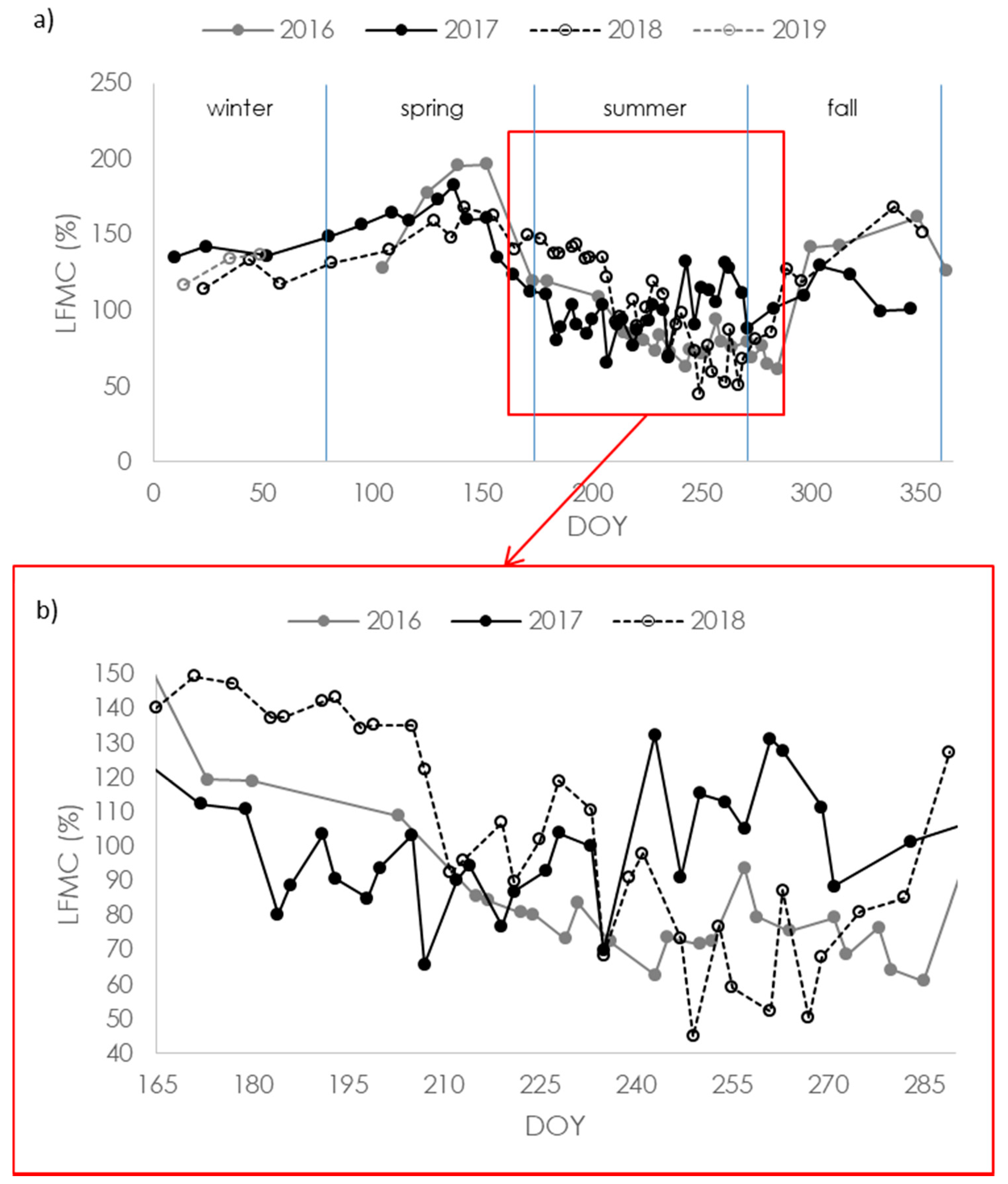
3.1. LFMC Variability and Remote Sensing Data

LFMC monitored in the field varied between years along the study period, especially during the fire season (15 June to 15 October). Maximum values were generally registered in spring, with the highest value in 2016 (196%), whereas minimum LFMC was observed in summer, with 44.9% as the lowest value registered in 2018 (Figure 2a). Differences between years were observed in LFMC values along the fire season (Figure 2b), which may be explained by the different meteorological conditions. Whereas the temperature regime between years was similar during the study period (April 2016 to February 2019), with an absolute maximum reaching 38 °C to 40 °C in summer (June/August) and an absolute minimum ranging −3 °C to −6 °C in winter (December/February), precipitation varied between years (Figure 3). A typical drought period occurred during the 2016 and 2018 fire seasons, but 2017 registered some storm rainfalls during the summer. However, the year 2018 was considerably wetter than in 2016 and 2017 mainly due to a higher amount of precipitation in spring (Figure 3).
Concerning remote sensing data, the time series available for the study period varied depending on the sensor and MODIS product used. The timelag between images and the sampling date was limited to a maximum of 2 days to compare with the field data. Both Sentinel-2 sensors were not fully operational in 2016, hence only 8 images from 2A (and non from 2B) were available in the study area, compared to 30 and 25 images for MODIS composite (MCD43A4) and non-composite (MOD09GA) products, respectively.
Outliers in SI for each surface reflectance source were checked in scatter plots and excluded from the modeling datasets (see an example in Appendix A, Figure A1). Final sample size was n = 120 for MCD43A4, n = 97 for MOD09GA and n = 71 for Sentinel-2. The range of field LFMC values included in both calibration and validation datasets for each sensor and MODIS product is shown in Table 2.

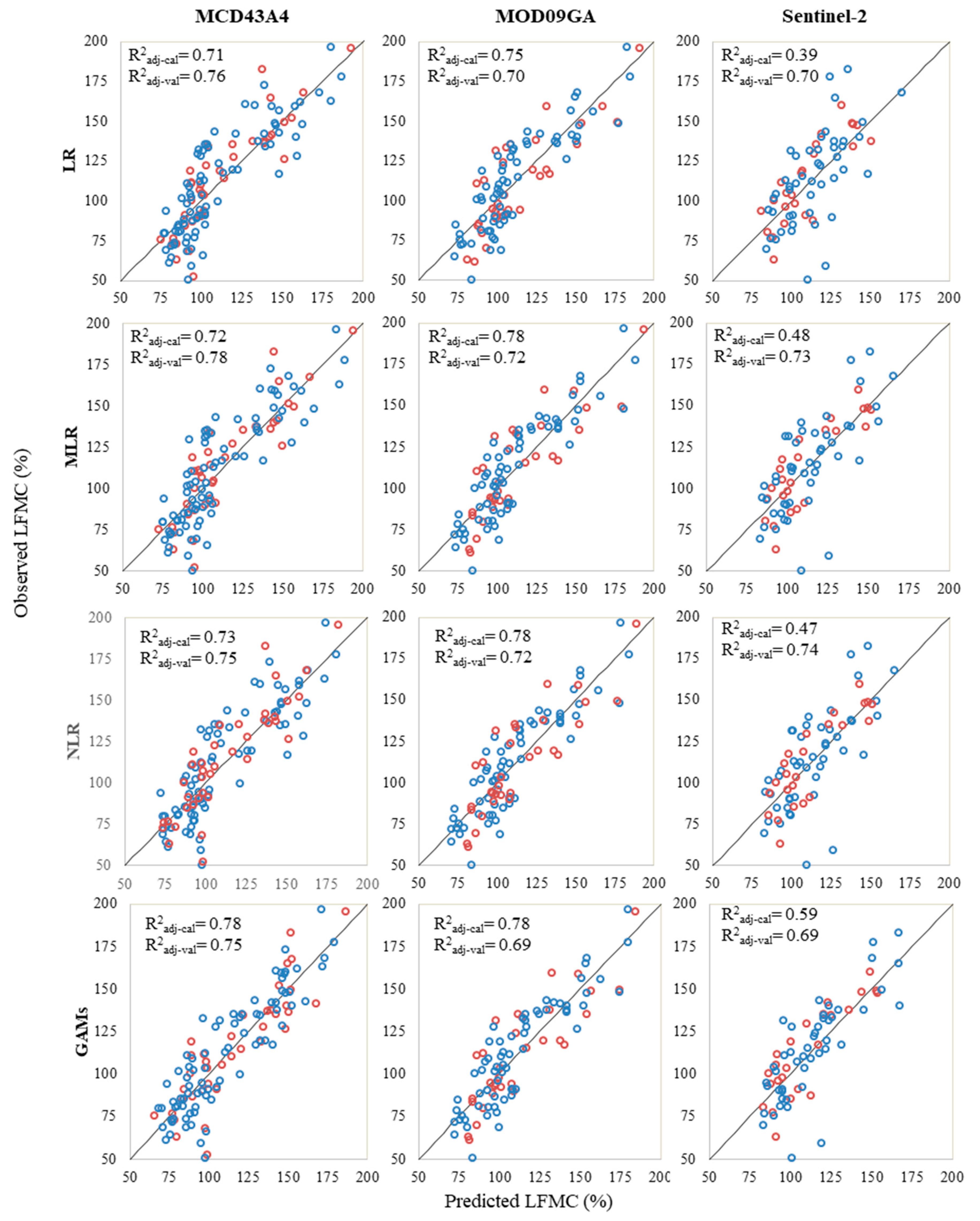
3.2. Comparison between Reflectance Source and Statistical Method

Most of the SI derived from MODIS and Sentinel-2 showed a high correlation with LFMC data (Table 3 and Table 4). For the composite product (MCD43A4), all indices had a significant linear relationship with LFMC (p-value < 0.01). The strongest correlations were found for NDVI, VARI, and VIgreen, with R2 from 0.70 to 0.71, RMSE ranging 17.9% to 18%, and MAE from 14.1% to 14.2%. The best MLR model included VIgreen, GVMI, and NDWI providing a very slight improvement compared to the simple regression models, but all parameters were not significant at the 0.05 level (Table 5).
The indices with higher correlation with LFMC from MOD09GA images were VARI and VIgreen, followed by NDVI and SAVI (Table 3). However, simple regression analysis only resulted in significant LR models for VARI (R2adj = 0.75, MAE = 12.9%) and VIgreen (R2adj = 0.73, MAE = 13.1%). A significant MLR model was found combining NDVI and VARI, with an increase in estimation accuracy compared to LR models (R2adj = 0.78 with MAE = 11.8%).
Regarding Sentinel-2, VARI and VIgreen also showed a higher correlation with LFMC (Table 4), but simple linear regression models had a poorer fit (R2adj < 0.40, MAE > 17%) (Table 5). In this case, the MRL model combining VARI and SAVI significantly improved linear regression results (R2adj = 0.48, MAE > 15.8%).
Concerning non-linear regression methods, the best formulation found was similar in all cases, including log(1 + VARI) as the main input variable, and either log(NDVI) or log(SAVI) for MODIS and Sentinel-2 images, respectively. GAMs models included similar SI indices as NLR models, but showing a higher R2adj and lower errors for the three types of surface reflectance source used, with R2adj > 0.78 for both MODIS products and R2adj = 0.58 for Sentinel-2. Details of the best models found for each fitting method and surface reflectance source are shown in Table 5.
Despite the fact that GAMs models showed the best goodness of fit and error for model calibration in all cases, the model performance with the independent datasets suggested that more simple formulations provide better validation results (Table 5). Linear regression methods had the best fit for MCD43A4 images, but NLR showed the lowest estimation error (12%) with a good model performance (R2adj > 0.75). For MOD09GA images, MLR and NLR showed similar validation results (R2adj > 0.72, MAE = 13%), although lower RMSE estimation errors for NLR model (<16%). NLR model provided the best validation results for Sentinel-2 images, with a good performance and estimation errors (R2adj = 0.74, RMSE = 13%, MAE = 11%). However, regarding critical moisture levels (LFMC < 80 %) there is a tendency to overestimate in all cases (Figure 4). Examples of spectral reflectance profiles derived from Sentinel-2 and both MODIS products comparing two different levels of moisture during the summer period (LFMC = 62% and LFMC = 109%) are shown in Appendix B (Figure A2).

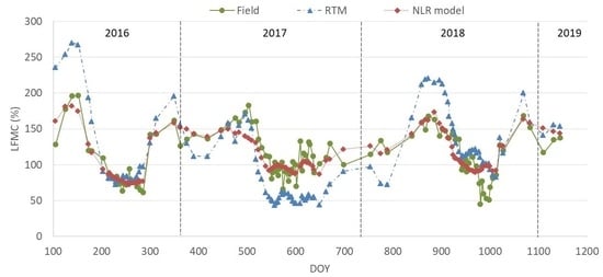
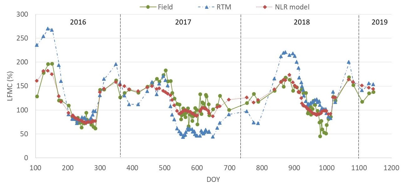
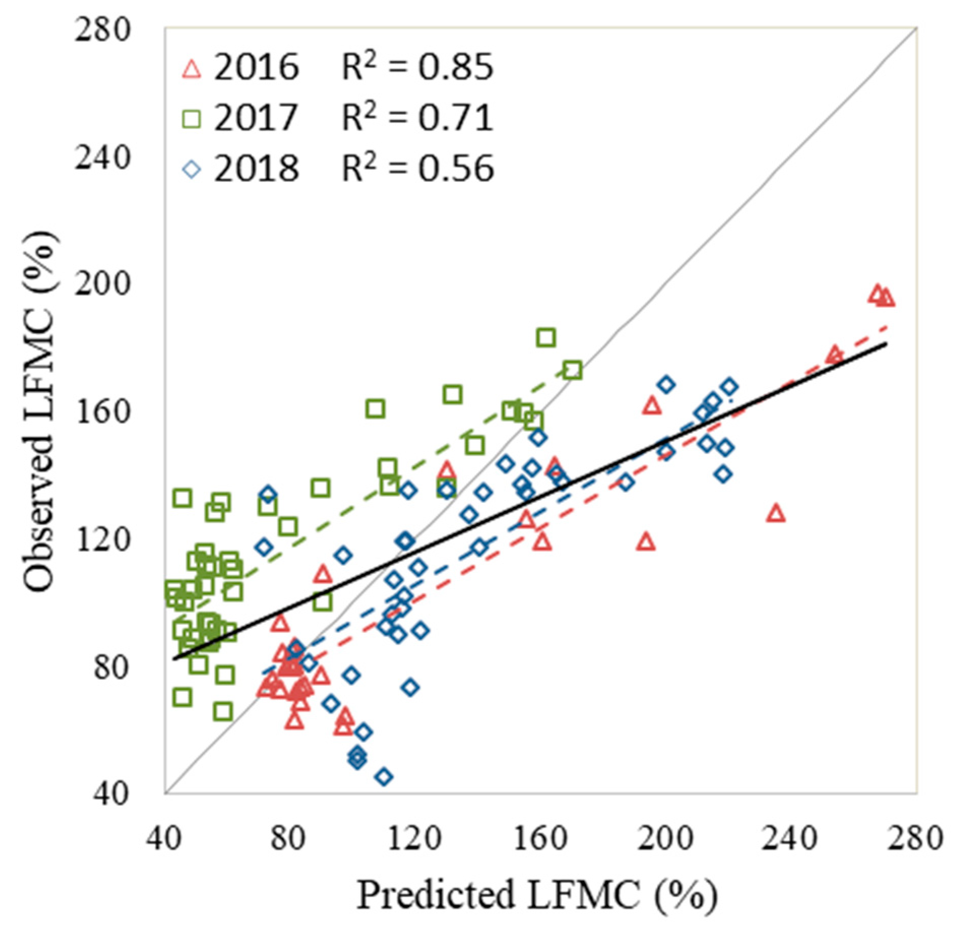
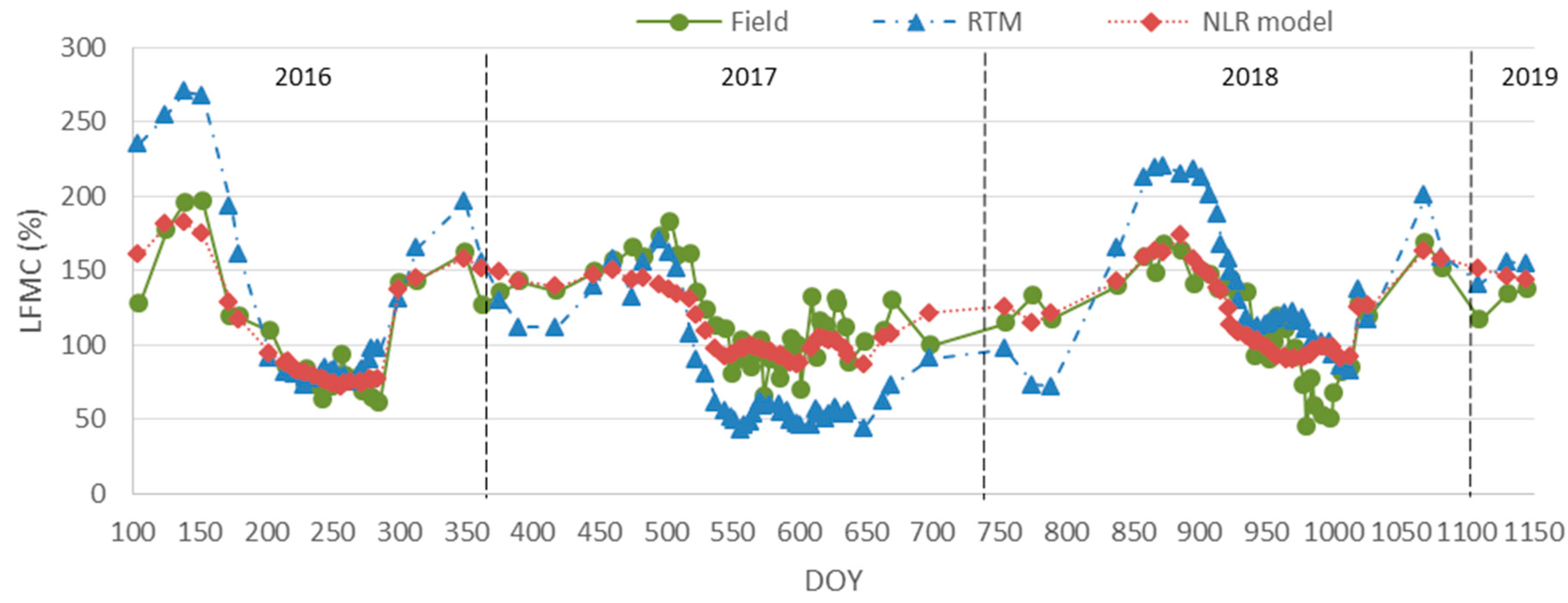
3.3. RTM Simulations

Predicted LFMC using RTM showed a significant correlation with observed LFMC but weaker compared to LFMC values derived from empirical models for the same type of MODIS product (Table 6). Stronger correlations between predictions and observations were found when assessing the performance of RTM simulations per year, with R2 between 0.56 and 0.85 (Table 6, Figure 5). However, these values were still lower than the equivalent statistics using the empirical models. Errors ranged from 36% to 43% (RMSE) and 25% to 38% (MAE), whereas NLR model validation for MCD43A4 images provided errors ranging 11% to 21% (RMSE) and 7% to 15% (MAE).
RTM simulations systematically overestimated the observed LFMC under a threshold value of 65% (Figure 5). When assessing the performance of the RTM per year, the slopes of the correlation between observed LFMC and RTM estimations are similar between years (Figure 5). However, estimated LFMC in 2017 always underpredicted the observed values, being also generally lower than estimations in 2016 and 2018 for the same field data. Temporal trends of LFMC along the study period showed that RTM simulations seemed to amplify either the increasing or decreasing LFMC values, thus resulting in higher overestimation or underestimation, respectively, of moisture levels compared to empirical modeling (Figure 6).

4. Discussion

Reflectance data from Sentinel-2 and two MODIS products (MOD09GA and MCD43A4) provided useful information for LFMC retrieval in C. ladanifer shrubland. Comparing the best models for both types of MODIS products, similar results were found for the composite product MCD43A4 (R2 = 0.75, MAE = 12%, RMSE = 17%) compared to non-composite product MOD09GA (R2 = 0.72, MAE = 13%, RMSE = 16%). These results are in the range of values reported by previous authors using empirical modeling for LFMC from MODIS composite products in different types of vegetation [19,21,22,23]. However, even though MCD43A4 is a daily product, reflectance data would not be valid for retrieving LFMC estimations at an operational level due to the timelag in image availability inherent to a 16-day composite. Moreover, image composite products tend to smooth LFMC variability in the short term, which hinders the identification of days with higher fire risk associated with anomalous extreme LFMC values (see Appendix B, Figure A2, for an example comparing spectral reflectance profiles derived from each type of product for two different field LFMC levels measured in the study area during the same summer period). This may be more relevant in areas covered by vegetation types including species that are more sensitive to LFMC variations in short periods of time, i.e., shrubland and grassland, compared to forests that do not generally change moisture contents within a few days.
Regarding the comparison of non-composite products between sensors, MODIS showed a considerably better performance in model calibration than Sentinel-2. It should be highlighted that, despite the worse fitting results obtained for Sentinel-2, the good performance observed with an independent validation dataset (R2 = 0.74, MAE = 11%, RMSE = 13%) suggests that the proposed NLR model seems robust enough to estimate LFMC in similar shrubland, at least within the range of values tested in this study (50–183%). These are good results, taking into account that errors of 10% in LFMC estimation from field measurements are generally acceptable according to fire management services. Nevertheless, lower LFMC values are extreme and anomalous values, and hence are less frequent in the sample for the three types of images. So, despite calibration and validations datasets are well balanced to represent the whole range of the LFMC in both the MODIS and Sentinel-2, the numbers of observations regarding extreme LFMC values are not as large as in the calibration. This is especially true in the case of Sentinel-2, where there is also a lower number of total samples. We hypothesize that as low LFMC values are more difficult to predict, validation in our models may, in turn, provide better results compared to the calibration dataset in most cases. In the particular case of Sentinel-2, only 3 data were available below the critical threshold of 80% in the validation, highlighting the need for longer time series that include more samples with lower LFMC values.
Regarding previous studies using Sentinel-2 data, our results are remarkably better than those obtained by Shu et al. [24], especially in terms of errors. However, we recognized that this could be due to the limited number of observations available in Shu et al. [24] study compared to the longer number of observations used in the present work. The finer spatial resolution of Sentinel-2 did not substantially increase model performance, at least for the monospecific shrubland site used in this manuscript. Consequently, the MOD09GA daily reflectance product may be recommended when near real-time estimations of LFMC are required. However, with both satellites 2A and 2B fully operational, it could be possible to retrieve LFMC from Sentinel-2 every 5 days or less, depending on the latitude (e.g., 2–3 days in the study area). Hence, Sentinel-2 may be a good alternative to MODIS if daily estimations are not a priority but higher spatial resolution is needed (e.g., patchy vegetation areas). Other authors proposed upscaling methods using multiple remote sensing data to provide higher temporal resolution, as reported by Adab et al. [48] to retrieve daily estimations of LFMC from Landsat and MODIS in a humid temperate forest. These authors first fitted empirical models based on spectral data derived from Landsat to predict LFMC measured at 30 m and then aggregated pixel values to 500 m using the nearest neighbor resampling method to perform PCA analysis and get daily LFMC estimations from MODIS data [48]. However, this method is not suitable when near-real-time estimations of vegetation moisture are required at a finer spatial resolution.
Comparing fitting methods for empirical modeling, validation results showed that although GAMs models had a better performance in terms of model calibration, simpler models can provide higher estimation accuracy. Namely, NLR formulation showed the best results in both MODIS and Sentinel-2 images, especially for the non-composite products (Table 5). The best NLR model for MODIS products (MCD43A4 and MOD09GA) included VARI and NDVI with a log-transformation. The Sentinel-2 model had a very similar NLR equation but included SAVI instead of NDVI.
The present study is in agreement with previous studies reporting VARI as the best SI to predict LFMC variation from MODIS images [21,22,23,26,29]. VARI is an SI based on reflectance from only visible wavelength bands (blue-green-red), but it has been reported to be very sensitive to chlorophyll and LAI variations associated with leaf drying [29]. Yebra et al. [29] observed that VARI provided the best correlation for C. ladanifer but offered the lowest for grasslands, being the only index with higher correlations for shrubs than for grasslands in their study. Our results showed that the combination of VARI with NDVI resulted in the best multivariate models for both MODIS products tested. Some authors have suggested that other SI improve model performance. For example, Peterson et al. [22] proposed a combination of VARI and VIgreen. Even though, in our case, VIgreen also explained well the variability of LFMC in the three types of surface reflectance sources, the high correlation found between VIgreen and VARI precluded the use of the former as an input in our models when the latter was included (Table 3). Stow et al. [21] reported the best empirical model with VARI and NDWI in California chaparral, whereas Caccamo et al. [23] found a better model performance combining VARI with NDII6 for Australian vegetation. Conversely, NDII6 and NDWI were among the indices with lower correlation in this study. VARI and NDVI are based on visible/NIR reflectance data, which is suitable for measuring greenness variations, whereas NDWI and NDII6 are supposed to be more sensitive to water content as they are based on NIR/SWIR reflectance [23]. Our results suggest that, since moisture variations affect C. ladanifer’s chlorophyll activity, greenness indices can effectively provide an indirect estimation of water content even though they do not include water absorption bands [29].
When comparing results between RTM and empirical modeling for the MODIS composite product (MCD43A4), NRL model provided better results than RTM simulations, especially regarding error level. Both RTM and empirical models showed higher accuracy assessing the performance per year than when including the complete time series. The best results were observed in 2016, with R2 of 0.85 and 0.95 and MAE of 25% and 7.5% for RTM and NLR empirical model, respectively. This shows that the effect of inter-annual variability on LFMC could be partly due to the different weather conditions occurring during the study period (Figure 3), especially regarding precipitation distribution [2,17]. Hence, further work is needed to disentangle the complex interactions between plant water status, soil moisture, and previous rainfalls [17,49]. Nevertheless, ecophysiological and weather data may be considered in order to improve model estimations [50,51].
Both approaches (empirical and RTM) tended to overestimate the lower LFMC values observed in the field, although with RTM simulations at a lower threshold (<65%) than empirical models (<80%). These values are below the 80% critical value considered by the fire management services in Spain for C. ladanifer and similar to other fire-prone shrubland fuels reported in previous studies. For example, the critical threshold considered in California chaparral varied from 60% to 79% [2,3,49]. Our results suggest that models should be further developed to improve estimations under these critical LFMC values. Our empirical models do not seem biased (Figure 4), but an enlarged calibration dataset with more reference values with LFMC < 60% would be strongly recommended to improve estimations at the highest flammability levels of C. ladanifer. However, despite the general trend to overpredict lower LFMC values, the proposed empirical models may be useful to identify when the critical threshold for high fire risk has been reached with reasonable accuracy in operational pre-alert systems.
Results in this study confirm that empirical modeling is an effective method to get reasonably accurate estimations of LFMC (MAE < 13%) at the local scale for fire-prone shrub species with high moisture variability, and under differing weather conditions when reliable field data is available for the calibration. With robust, long-term databases of LFMC measurements recently becoming open-access [17,18], the empirical approach is still an efficient one that should be considered for remote sensing estimation of vegetation moisture dynamics of the main species affected by wildfire at local scales. Empirical modeling may be successfully applied to estimate LFMC of indicator species useful for wildfire risk rating, as presented in this study. The adequacy of using indicator species for LFMC monitoring has already been highlighted by other authors [49]. Nevertheless, this approach may also be used to retrieve LFMC of mixed vegetation, provided that the cover fraction of dominant species would be registered to obtain a representative LFMC value at an appropriate scale according to the equivalent pixel value estimated by each sensor [19].
Conversely, current results regarding RTM suggest that estimation accuracy should be further improved to be efficiently used at an operational level. Although RTM provided less tendency to systematically overpredict lower moisture values compared to empirical models, the estimation error (MAE > 25%) may somehow hinder its use when more detailed LFMC monitoring would be required. Calibration and validation are on-going to adapt RTM simulations to reflectance from different types of sensors, including Sentinel-2. Hence, more operational applications of RTM are expected in the near future, which may favor the implementation of advanced fire danger rating systems at a global level.

5. Conclusions

This is the first study to date that carried out a comprehensive analysis of Sentinel-2 capability for LFMC estimation in comparison to MODIS products (composite and non-composite images) and different retrieval methods (empirical vs. RTM). Our results suggest that empirical modeling is an effective method to monitor LFMC dynamics in fire-prone shrubland with operational remote sensing products at a reasonable accuracy for wildfire danger rating at a local scale. Empirical models derived from Sentinel-2 and MODIS data provide similar results in terms of fitting and error level. VARI is the best spectral index for LFMC retrieval in C. ladanifer shrubland, showing an improved model performance in a non-linear formulation with NDVI or SAVI, depending on the type of sensor used. RTM simulations are a suitable alternative for LFMC estimation at a regional or global scale but do not yet provide the same accuracy level as empirical models at a local scale. Both RTM simulations and empirical models tend to overestimate the lower LFMC values observed in the field and should be further improved to get better estimations of vegetation moisture under the critical levels considered as more extreme flammability conditions for wildfires.

Author Contributions

Conceptualization, E.M., J.L.T., J.M., M.G., C.H.; methodology, E.M., M.Y., M.G.-C., N.A., J.L.T., J.M., M.G., C.H.; validation, E.M, M.Y.; formal analysis, E.M, M.Y, M.G.-C., N.A.; investigation, E.M., M.Y., M.G.-C., N.A., J.M., C.H.; writing—original draft preparation, E.M.; writing—review and editing, E.M., M.Y., J.L.T., J.M., M.G., C.H.; visualization, E.M.; supervision, E.M., M.Y., J.L.T., J.M., C.H.; project administration, E.M., J.L.T., J.M., C.H.; funding acquisition, E.M., J.L.T., J.M., M.G., C.H. All authors have read and agreed to the published version of the manuscript.

Funding

This research was partially funded by the Spanish National Research Institute for Agriculture (INIA) through projects VIS4FIRE (RTA2017-00042-C05-01) and GEPRIF (RTA2014-00011-C06-06), and co-funded by the EU-FEDER program. Eva Marino’s participation was also partially funded by a postdoctoral grant from the Spanish Ministry of Economy and Competitiveness (Torres-Quevedo program) supported by European Social Fund (ESF).

Acknowledgments

We are grateful to the firefighting service from Comunidad de Madrid for providing field data. We also thank Francisco Rodríguez-Sánchez for his helpful comments on GAM models.

Conflicts of Interest

The authors declare no conflict of interest.

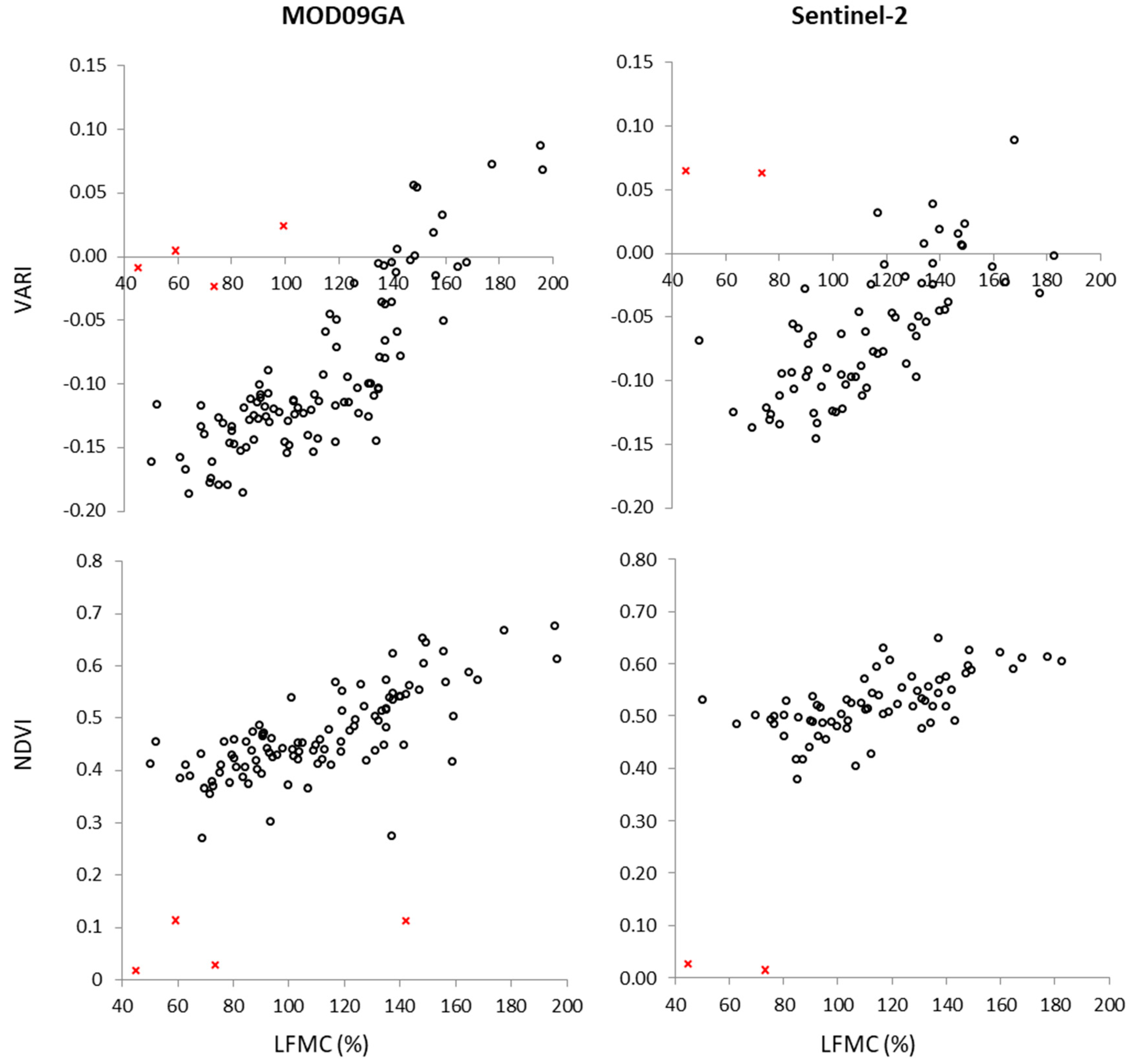
Appendix A. Example of Outlier Detection in Spectral Indices Described in Section 3.1

Figure A1. Examples of scatter plots of NDVI and VARI derived from MOD09GA and Sentinel-2. Ouliers detected and excluded from the modelling datasets are depicted as red crosses.
Remotesensing 12 02251 g0a1

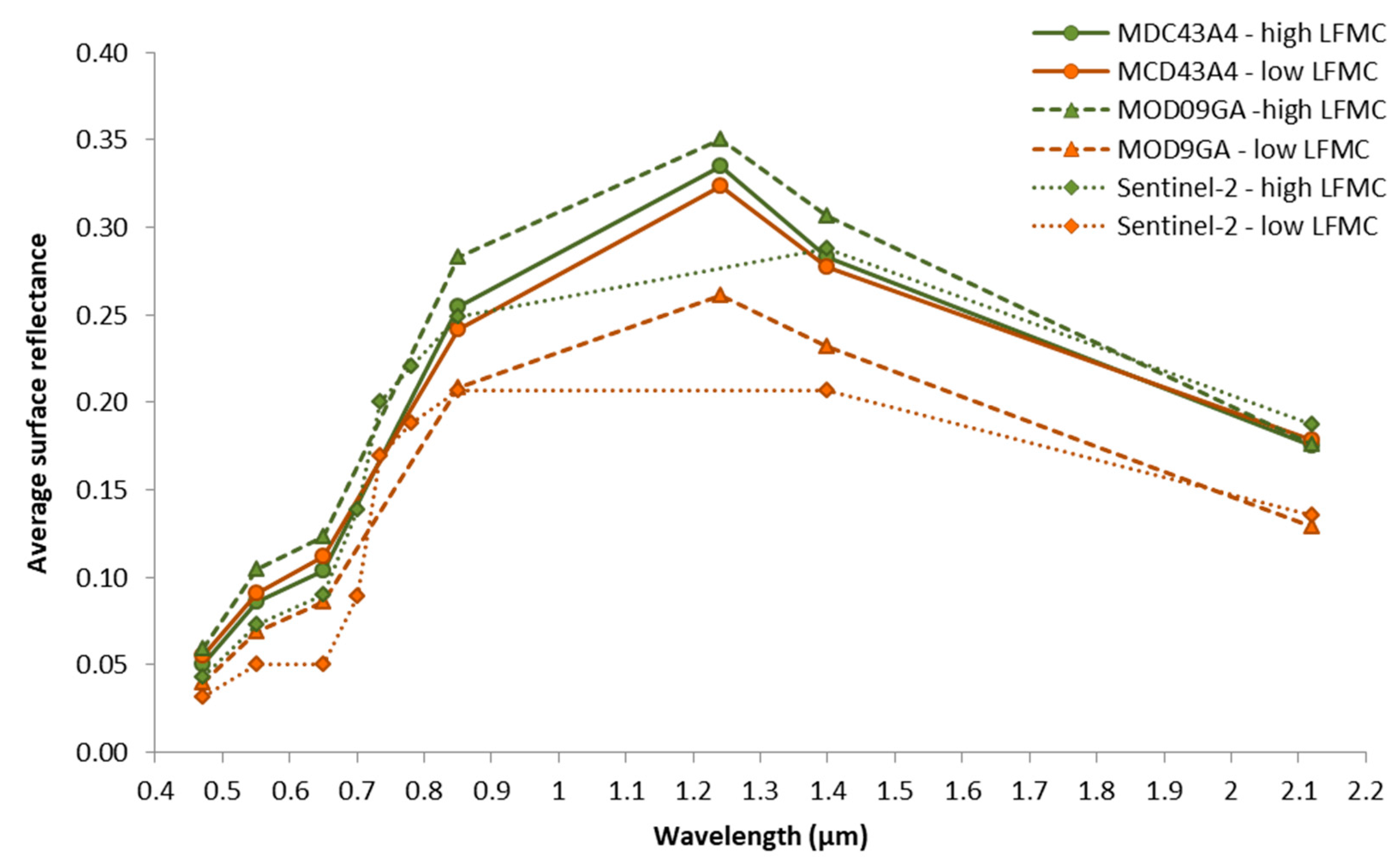
Appendix B. Examples of Spectral Reflectance Profiles Derived from Sentinel-2 and Both MCD43A4 and MOD09GA MODIS Products

Figure A2 depicts the spectral reflectance profiles for two sampling dates during the summer of 2016 (21 of July and 30 of August, respectively) with contrasting C. ladanifer’s LFMC (109% and 62%). Reflectance values obtained from Sentinel-2 and the MODIS daily reflectance product (MOD09GA) for the LFMC = 109% and LFMC = 62% show higher variability than those obtained from the 16-day MODIS composite product (MCD43A4). In the higher moisture case (109%), estimated LFMC is 109% and 94% using the best empirical models (NLR) derived from Sentinel-2 and MODIS products, respectively, whereas 91% using RTM simulations. In the lower moisture case (62%) all models overestimated observed LFMC, with empirical models providing values of 92% with Sentinel-2, 81% with MOD09GA and 77% with MCD43A4, whereas a value of 82% is estimated with RTM simulations. The similar trend in reflectance spectra observed between both LFMC levels that basically vary only in magnitude but not in shape (as it is expected as wetter vegetation has higher values in NIR and lower values in SWIR than dryer vegetation), might be the cause of the overestimation of the LFMC on the 30th August and be influenced by the effect of soil reflectance during the dry summer period. Nevertheless, the expected variability in spectral reflectance profiles is observed in samples with larger differences in LFMC along the year.
Figure A2. Comparison of spectral reflectance profiles from Sentinel-2 and the composite (MCD43A4) and non-composite (MOD09GA) MODIS products for dates in the 2016 summer period with contrasting values of field measured LFMC: high LFMC = 109% (21 July 2016) and low LFMC = 62% (30 August 2016).
Remotesensing 12 02251 g0a2

References

  1. Chuvieco, E.; Gonzalez, I.; Verdú, F.; Aguado, I.; Yebra, M. Prediction of fire occurrence from live fuel moisture content measurements in a Mediterranean ecosystem. Int. J. Wildland Fire 2009, 18, 430. [Google Scholar] [CrossRef]
  2. Dennison, P.E.; Moritz, M.A. Critical live fuel moisture in chaparral ecosystems: A threshold for fire activity and its relationship to antecedent precipitation. Int. J. Wildland Fire 2009, 18, 1021–1027. [Google Scholar] [CrossRef]
  3. Weise, D.R.; Zhou, X.; Sun, L.; Mahalingam, S. Fire spread in chaparral- ‘go or no go?’. Int. J. Wildland Fire 2005, 14, 99–106. [Google Scholar] [CrossRef]
  4. Marino, E.; Dupuy, J.L.; Pimont, F.; Guijarro, M.; Hernando, C.; Linn, R. Fuel bulk density and fuel moisture content effect on fire rate of spread: A comparison between FIRETEC model predictions and experimental results in shrub fuels. J. Fire Sci. 2012, 30, 277–299. [Google Scholar] [CrossRef]
  5. Rossa, C.G.; Veloso, R.; Fernandes, P.M. A laboratory-based quantification of the effect of live fuel moisture content on fire spread rate. Int. J. Wildland Fire 2016, 25, 569–573. [Google Scholar] [CrossRef] [Green Version]
  6. Agee, J.K.; Wright, C.S.; Williamson, N.; Huff, M.H. Foliar moisture content of Pacific Northwest vegetation and its relation to wildland fire behavior. Forest Ecol. Manag. 2002, 167, 57–66. [Google Scholar] [CrossRef]
  7. Alexander, M.E.; Cruz, M.G. Assessing the effect of foliar moisture content on the spread rate of crown fires. Int. J. Wildland Fire 2013, 22, 415–427. [Google Scholar] [CrossRef]
  8. Ruffault, J.; Curt, T.; Martin-StPaul, N.K.; Moron, V.; Trigo, R.M. Extreme wildfire events are linked to global-change-type droughts in the northern Mediterranean. Nat. Hazards Earth Syst. Sci. 2018, 18, 847–856. [Google Scholar] [CrossRef] [Green Version]
  9. Spinosi, J.; Barbosa, P.; Bucchgnai, E.; Cassano, J.; Cavazos, T.; Christensen, J.H.; Christensen, O.B.; Coppola, E.; Evans, J.; Giorgi, F.; et al. Future Global Meteorological Drought Hot Spots: A Study Based on CORDEX Data. J. Clim. 2020, 33, 3635–3661. [Google Scholar] [CrossRef]
  10. Moreira, F.; Viedma, O.; Arianoutsou, M.; Curt, T.; Koutsias, N.; Rigolot, E.; Barbati, A.; Corona, P.; Vaz, P.; Xanthopoulos, G.; et al. Landscape–wildfire interactions in southern Europe: Implications for landscape management. J. Environ. Manag. 2011, 92, 2389–2402. [Google Scholar] [CrossRef] [Green Version]
  11. Pausas, J.G.; Fernández-Muñoz, S. Fire regime changes in the Western Mediterranean Basin: From fuel-limited to drought-driven fire regime. Clim. Chang. 2012, 10, 215–226. [Google Scholar] [CrossRef] [Green Version]
  12. Linn, R.; Reisner, J.; Colman, J.J.; Winterkamp, J. Studying wildfire behavior using FIRETEC. Int. J. Wildland Fire 2002, 11, 233–246. [Google Scholar] [CrossRef]
  13. Finney, M.A. FARSITE: Fire Area Simulator–Model Development and Evaluation. In USDA Forest Service, Rocky Mountain Research Station; Research Paper RMRS-RP-4 Revised: Fort Collins, CO, USA, 2004. [Google Scholar]
  14. Finney, M.A. An overview of FlamMap fire modelling capabilities. In Proceedings of the ‘Fuels Management–How to Measure Success: Conference Proceedings’, Portland, OR, USA, 28–30 March 2006; Andrews, P.L., Butler, B.W., Eds.; USDA Forest Service, Rocky Mountain Research Station, Proceedings RMRS-P 41: Fort Collins, CO, USA, 2006; pp. 213–220. [Google Scholar]
  15. García, M.; Riaño, D.; Yebra, M.; Salas, J.; Cardil, A.; Monedero, S.; Ramirez, J.; Martín, M.P.; Vilar, L.; Gajardo, J.; et al. A Live Fuel Moisture Content Product from Landsat TM Satellite Time Series for Implementation in Fire Behavior Models. Remote Sens. 2020, 12, 1714. [Google Scholar] [CrossRef]
  16. Chuvieco, E.; Aguado, I.; Salas JGarcia, M.; Yebra, M.; Oliva, P. Satellite Remote Sensing Contributions to Wildland Fire Science and Management. Curr. For. Rep. 2020, 6, 81–96. [Google Scholar] [CrossRef]
  17. Martin-StPaul, N.; Pimont, F.; Dupuy, J.L.; Rigolot, E.; Ruffault, J.; Fargeon, H.; Cabane, E.; Duché, Y.; Savazzi, R.; Toutchkov, M. Live fuel moisture content (LFMC) time series for multiple sites and species in the French Mediterranean area since 1996. Ann. For. Sci. 2018, 75, 57. [Google Scholar] [CrossRef] [Green Version]
  18. Yebra, M.; Scortechini, G.; Badi, A.; Beget, M.E.; Boer, M.M.; Bradstock, R.; Chuvieco, E.; Danson, F.M.; Dennison, P.; de Dios, V.R.; et al. Globe-LFMC, a global plant water status database for vegetation ecophysiology and wildfire applications. Nat. Sci. Data 2019, 6, 155. [Google Scholar] [CrossRef] [Green Version]
  19. Yebra, M.; Dennison, P.E.; Chuvieco, E.; Riaño, D.; Zylstra, P.; Hunt ERJr Danson, F.M.; Qi, Y.; Jurdao, S. A global review of remote sensing of live fuel moisture content for fire danger assessment: Moving towards operational products. Remote Sens. Environ. 2013, 136, 455–468. [Google Scholar] [CrossRef]
  20. Dennison, P.E.; Roberts, D.A.; Peterson, S.H.; Rechel, J. Use of Normalized Difference Water Index for monitoring live fuel moisture. Int. J. Remote Sens. 2005, 26, 1035–1042. [Google Scholar] [CrossRef]
  21. Stow, D.; Madhura, N.; Kaiser, J. Time series of chaparral live fuel moisture maps derived from MODIS satellite data. Int. J. Wildland Fire 2006, 15, 347–360. [Google Scholar] [CrossRef]
  22. Peterson, S.; Roberts, D.A.; Dennison, P.E. Mapping live fuel moisture with MODIS data: A multiple regression approach. Remote Sens. Environ. 2008, 112, 4272–4284. [Google Scholar] [CrossRef]
  23. Caccamo, G.; Chisholm, L.A.; Bradstock, R.A.; Puotinen, M.L.; Pippen, B.G. Monitoring live fuel moisture content of heathland, shrubland and sclerophyll forest in south-eastern Australia using MODIS data. Int. J. Wildland Fire 2012, 21, 257–269. [Google Scholar] [CrossRef]
  24. Shu, Q.; Quan, X.; Yebra, M.; Liu, X.; Wang, L.; Zhang, Y. Evaluating the Sentinel-2A satellite data for fuel moisture content retrieval. In Proceedings of the IEEE International Geoscience and Remote Sensing Symposium, Yokohama, Japan, 28 July–2 August 2019; pp. 9416–9419. [Google Scholar]
  25. Tanase, M.A.; Panciera, R.; Lowell, K.; Aponte, C. Monitoring live fuel moisture in semiarid environments using L-band radar data. Int. J. Wildland Fire 2015, 24, 560–572. [Google Scholar] [CrossRef]
  26. Fan, L.; Wigneron, J.P.; Xiao, Q.; Al-Yaari, A.; Wen, J.; Martin-St Paul, N.; Dupuy, J.L.; Pimont, F.; Al Bitar, A.; Fernandez-Moran, R.; et al. Evaluation of microwave remote sensing for monitoring live fuel moisture content in the Mediterranean region. Remote Sens. Environ. 2018, 205, 210–223. [Google Scholar] [CrossRef]
  27. Wang, L.; Quan, X.; He, B.; Yebra, M.; Xing, M.; Liu, X. Assessment of the dual polarimetric Sentinel-1A data for forest fuel moisture content estimation. Remote Sens. 2019, 11, 1568. [Google Scholar] [CrossRef] [Green Version]
  28. Hao, X.J.; Qu, J.J. Retrieval of real-time live fuel moisture content using MODIS measurements. Remote Sens. Environ. 2007, 108, 130–137. [Google Scholar] [CrossRef]
  29. Yebra, M.; Chuvieco, E.; Riaño, D. Estimation of live Fuel Moisture Content from MODIS images for fire risk assessment. Agric. For. Meteorol. 2008, 148, 523–536. [Google Scholar] [CrossRef]
  30. Yebra, M.; Chuvieco, E. Linking ecological information and radiative transfer models to estimate fuel moisture content in the Mediterranean region of Spain: Solving the ill-posed inverse problem. Remote Sens. Environ. 2009, 113, 2403–2411. [Google Scholar] [CrossRef]
  31. Jurdao, S.; Yebra, M.; Guerschman, J.P.; Chuvieco, E. Regional estimation of woodland moisture content by inverting Radiative Transfer Models. Remote Sens. Environ. 2013, 132, 59–70. [Google Scholar] [CrossRef]
  32. Fosberg, M.A.; Deeming, J.E. Derivation of the 1- and 10-hour Timelag Fuel Moisture Calculation for Fire Danger Rating. In USDA Forest Service, Rocky Mountain Forest and Range Experiment Station; Research Paper RM-207; Rocky Mountain Forest and Range Experiment Station: Fort Collins, CO, USA, 1971; 10p. [Google Scholar]
  33. Louis, J.; Debaecker, V.; Pflug, B.; Main-Knorn, M.; Bieniarz, J.; Mueller-Wilm, U.; Cadau, E.; Gascon, F. Sentinel-2 Sen2Cor: L2A Processor for Users. In Proceedings of the Living Planet Symposium, Prague, Czech Republic, 9–13 May 2016; Ouwehand, L.L., Ed.; ESA-SP: São Paulo, Brazil, 2016; p. 91, ISBN 978-92-9221-305-3. [Google Scholar]
  34. Rouse, J.W., Jr.; Haas, R.W.; Schell, J.A.; Deering, D.H.; Harlan, J.C. Monitoring the Vernal Advancement and Retrogradation (Greenwave Effect) of Natural Vegetation; Type III Final Report; NASA/GSFC: Greenbelt, MD, USA, 1974.
  35. Hardisky, M.A.; Klemas, V.; Smart, R.M. The influence of soil salinity, growth form, and leaf moisture on the spectral radiance of Spartina alterniflora canopies. Photogramm. Eng. Remote Sens. 1983, 49, 77–83. [Google Scholar]
  36. Ceccato, P.; Flasse, S.; Gregoire, J.M. Designing a spectral index to estimate vegetation water content from remote sensing data: Part 2. Validation and applications. Remote Sens. Environ. 2002, 82, 198–207. [Google Scholar] [CrossRef]
  37. Gao, B.C. NDWI. A normalized difference water index for remote sensing of vegetation liquid water from space. Remote Sens. Environ. 1996, 58, 257–266. [Google Scholar] [CrossRef]
  38. Huete, A.; Didan, K.; Miura, T.; Rodriguez, E.P.; Gao, X.; Ferreira, L.G. Overview of the radiometric and biophysical performance of the MODIS vegetation indices. Remote Sens. Environ. 2002, 83, 195–213. [Google Scholar] [CrossRef]
  39. Huete, A.R. A soil-adjusted vegetation index (SAVI). Remote Sens. Environ. 1988, 25, 295–309. [Google Scholar] [CrossRef]
  40. Gitelson, A.; Kaufmam, J.Y.; Stark, R.; Rundquist, D. Novel algorithms for remote estimation of vegetation fraction. Remote Sens. Environ. 2002, 80, 76–87. [Google Scholar] [CrossRef] [Green Version]
  41. Tucker, C.J. Red and photographic infrared linear combinations for monitoring vegetation. Remote Sens. Environ. 1979, 8, 127–150. [Google Scholar] [CrossRef] [Green Version]
  42. R Core Team. R: A Language and Environment for Statistical Computing; URL: R Foundation for Statistical Computing: Vienna, Austria, 2016. Available online: https://www.gbif.org/tool/81287/r-a-language-and-environment-for-statistical-computing (accessed on 10 July 2020).
  43. Yebra, M.; Quan, X.; Riaño, D.; Rozas, P.; van Dijk, A.; Cary, J.K. A fuel moisture content and flammability monitoring methodology for continental Australia based on optical remote sensing. Remote Sens. Environ. 2018, 212, 260–272. [Google Scholar] [CrossRef]
  44. Jacquemoud, S.; Baret, F. PROSPECT: A model of leaf optical properties spectra. Remote Sens. Environ. 1990, 34, 75–91. [Google Scholar] [CrossRef]
  45. Verhoef, W. Light scattering by leaf layers with application to canopy reflectance modeling: The SAIL model. Remote Sens. Environ. 1984, 16, 125–141. [Google Scholar] [CrossRef] [Green Version]
  46. Kuusk, A. The Hot Spot Effect in Plant Canopy Reflectance. In Photon-Vegetation Interactions; Myneni, R., Ross, J., Eds.; Springer: Berli/Heidelberg, Germany, 1991; pp. 139–159. [Google Scholar]
  47. Jurdao, S.; Yebra, M.; Chuvieco, E. Live Fuel Moisture Content Derived from Remote Sensing Estimates in Temperate Shrublands and Grasslands. In Earthzine; IEEE Oceanic Engineering Society, 2013; Available online: https://earthzine.org/live-fuel-moisture-content-derived-from-remote-sensing-estimates-in-temperate-shrublands-and-grasslands/ (accessed on 24 October 2013).
  48. Adab, H.; Kanniah, K.D.; Beringer, J. Estimating and up-scaling fuel moisture and leaf dry matter content of a temperate humid forest using multi resolution remote sensing data. Remote Sens. 2016, 8, 961. [Google Scholar] [CrossRef] [Green Version]
  49. Pivovaroff, A.L.; Emery, N.; Sharifi, M.R.; Witter, M.; Keeley, J.E.; Rundel, P.W. The effect of ecophysiological traits on live fuel moisture content. Fire 2019, 2, 28. [Google Scholar] [CrossRef] [Green Version]
  50. Garcia, M.; Chuvieco, E.; Nieto, H.; Aguado, I. Combining AVHRR and meteorological data for estimating live fuel moisture content. Remote Sens. Environ. 2008, 112, 3618–3627. [Google Scholar] [CrossRef]
  51. Nolan, R.H.; Resco de Dios, V.; Boer, M.M.; Caccamo, G.; Goulden, M.L.; Bradstock, R.A. Predicting dead fine fuel moisture at regional scales using vapour pressure deficit from MODIS and gridded weather data. Remote Sens. Environ. 2016, 174, 100–108. [Google Scholar] [CrossRef] [Green Version]
Figure 1. Location of the study area and example of a field sample collected in the C. ladanifer shrubland.
Remotesensing 12 02251 g001
Figure 2. LFMC of C. ladanifer monitored in the field: (a) from April 2016 to February 2019 and (b) during the fire season (15 June (DOY = 166) to 15 October (DOY = 288)).
Remotesensing 12 02251 g002
Figure 3. Comparison of the temperature regime (average maximum, mean and minimum values) and precipitation distribution between years during the study period.
Remotesensing 12 02251 g003
Figure 4. Observed vs. predicted values of LFMC using the best empirical model obtained for each type of surface reflectance source and method used (LR, MLR, NLR, and GAMs). Blue and red circles depict calibration and validation data, respectively.
Remotesensing 12 02251 g004
Figure 5. Observed vs. predicted values of LFMC obtained from RTM with correlation lines for the complete dataset (continuous black) and each year (dashed color lines).
Remotesensing 12 02251 g005
Figure 6. Comparison of C. ladanifer LFMC values from field monitoring and estimations from RTM and an empirical model (NLR).
Remotesensing 12 02251 g006
Table 1. Spectral indices obtained from MODIS and Sentinel-2 data. ρx is the reflectance in band x; NIR, near-infrared; SWIR, short wave infrared; n.a., not applicable.
IndexFormulationMODIS BandsSentinel-2 BandsRefer.
Normalized Difference Vegetation Index N D V I = ρ N I R ρ r e d ρ N I R + ρ r e d ρ N I R = ρ 2
ρ r e d = ρ 1
ρ N I R = ρ 8 A
ρ r e d = ρ 4
[34]
Normalized Difference Infrared Index N D I I = ρ N I R ρ S W I R ρ N I R + ρ S W I R ρ N I R = ρ 2
ρ S W I R = ρ 6 (NDII6)
ρ N I R = ρ 2
ρ S W I R = ρ 7 (NDII7)
ρ N I R = ρ 8 A
ρ S W I R = ρ 11
[35]
Global Vegetation Moisture Index G V M I = ( ρ N I R + 0.1 ) ( ρ S W I R + 0.02 ) ( ρ N I R + 0.1 ) + ( ρ S W I R + 0.02 ) ρ N I R = ρ 2
ρ S W I R = ρ 6
ρ N I R = ρ 8 A
ρ S W I R = ρ 11
[36]
Normalized Difference Water Index N D W I = ρ N I R 2 ρ N I R 1 ρ N I R 2 + ρ N I R 1 ρ N I R 2 = ρ 2
ρ N I R 1 = ρ 5
n.a.[37]
Normalized Difference Red-Edge Index N D I 45 = ρ r e d e d g e ρ r e d ρ r e d e d g e + ρ r e d n.a. ρ r e d = ρ 4
ρ r e d e d g e = ρ 5
Enhanced Vegetation Index E V I = 2.5 ( ρ N I R ρ r e d ) ρ N I R + 6 ( ρ r e d ) 7.5 ( ρ b l u e ) + 1 ρ N I R = ρ 2
ρ r e d = ρ 1
ρ b l u e = ρ 3
ρ N I R = ρ 8 A
ρ r e d = ρ 4
ρ b l u e = ρ 2
[38]
Soil Adjusted Vegetation Index S A V I = ( 1 + 0.5 ) ( ρ N I R ρ r e d ) ( ρ N I R + ρ r e d + 0.5 ) ρ N I R = ρ 2
ρ r e d = ρ 1
ρ N I R = ρ 8 A
ρ r e d = ρ 4
[39]
Visible Atmospherically Resistant Index V A R I = ρ g r e e n ρ r e d ρ g r e e n + ρ r e d ρ b l u e ρ g r e e n = ρ 4
ρ r e d = ρ 1
ρ b l u e = ρ 3
ρ g r e e n = ρ 3
ρ r e d = ρ 4
ρ b l u e = ρ 2
[40]
Vegetation Index—Green V I g r e e n = ρ g r e e n ρ r e d ρ g r e e n + ρ r e d ρ g r e e n = ρ 4
ρ r e d = ρ 1
[41]
Table 2. Sample size (n) and the range of LFMC field values available in model calibration and validation datasets for each surface reflectance source.
ImageCalibrationValidation
nLFMC Range (%)nLFMC Range (%)
MCD43A48050–1974045–196
MOD09GA6550–1963261–195
Sentinel-24750–1832463–160
Table 3. Pearson correlation matrix for each MODIS product calibration dataset. All correlations significant at p-value < 0.001.
ProductSILFMCNDVINDII6NDII7GVMINDWIEVISAVIVARI
MCD43A4NDVI0.844
NDII60.4610.578
NDII70.5900.7300.647
GVMI0.6780.8520.6400.918
NDWI0.6710.7510.6190.8540.804
EVI0.7120.7990.6600.7750.7420.875
SAVI0.7280.8160.6540.7580.7360.8680.999
VARI0.8460.9610.6160.7180.8380.7350.8030.815
VIgreen0.8430.9610.6220.7290.8460.7410.8070.8171.000
MOD09GANDVI0.761
NDII60.6300.633
NDII70.5660.5810.949
GVMI0.6300.6331.0000.949
NDWI0.5960.4770.6990.7110.699
EVI0.7140.5060.6830.6390.6830.677
SAVI0.7611.0000.6330.5810.6330.4770.506
VARI0.8660.7380.6820.5920.6820.6730.7930.738
VIgreen0.8590.7240.6890.5970.6890.6810.7940.7240.999
Table 4. Pearson correlation matrix for Sentinel-2 calibration dataset. Significance level: * p-value < 0.05, ** p-value < 0.01, *** p-value < 0.001.
SILFMCNDVINDIINDI45GVMIEVISAVIVARI
NDVI0.428 **
NDII0.445 **0.311 *
NDI450.382 **0.959 ***0.274
GVMI0.1590.307 **0.2250.166
EVI0.523 ***0.338 *0.385 **0.396 **0.338 **
SAVI0.458 **0.708 ***0.1780.743 ***0.0130.729 ***
VARI0.637 ***0.456 **0.825 ***0.408 **0.233 *0.407 **0.239
VIgreen0.624 ***0.432 **0.815 ***0.375 **0.251 *0.392 **0.2210.995 ***
Table 5. Best empirical models fitted for each sensor, MODIS product, and method used. R2adj, adjusted R2; MAE, mean absolute error; RMSE, root mean square error.
Sensor/MODIS ProductModel FormulationParametersp-valueCalibrationValidation
R2 adjRMSE (%)MAE (%)R2 adjRMSE (%)MAE (%)
MCD43A4LRFMC = a+b·VARIa = 152.676
b = 487.731
< 0.0001
< 0.0001
0.71117.8714.140.75617.2912.32
MLRFMC = a+b· VIgreen +c·GVMI+d·NDWIa = 198.73
b = 715.49
c = −149.33
d = 234.32
< 0.0001
< 0.0001
0.0556
0.0534
0.71817.5413.880.78216.3112.12
NLRFMC = a+b·log(1+VARI)+c·log(NDVI)a = 203.5
b = 253.5
c = 88.61
< 0.0001
0.0195
0.0441
0.72917.2013.580.75217.3612.05
GAMsFMC = f(a,s(VARI),s(NDVI))a = 111.23
s(VARI)
s(NDVI)
< 0.0001
< 0.0001
0.0012
0.78115.0511.910.75016.5412.47
MOD09GALRFMC = a+b·VARIa = 153.352
b = 430.273
< 0.0001
< 0.0001
0.75015.4612.960.69617.0114.52
MLRFMC = a+b·VARI+c·NDVIa = 96.18
b = 331.77
c = 101.37
< 0.0001
< 0.0001
0.0032
0.78314.4111.830.72116.2413.35
NLRFMC = a+b·log(1+VARI)+c·log(NDVI)a = 178.00
b = 325.36
c = 42.07
< 0.0001
< 0.0001
0.0034
0.78014.3011.660.72015.96 13.39
GAMsFMC = f(a,s(VARI),s(NDVI))a = 111.65
s(VARI)
s(NDVI)
< 0.0001
< 0.0001
0.0157
0.78413.9811.470.68615.9913.33
Sentinel-2LRFMC = a+bVARIa = 136.320
b = 372.929
< 0.0001
< 0.0001
0.39322.8417.330.70214.7312.69
MLRFMC = a+b·VARI+c·SAVIa = 60.57
b = 333.05
c = 390.22
0.0242
< 0.0001
0.0048
0.48220.8515.770.73213.6511.21
NLRFMC = a+b·log(1+VARI)+c·log(SAVI)a = 244.53
b = 327.81
c = 65.41
< 0.0001
< 0.0001
0.0075
0.47320.8115.460.73713.5411.11
GAMsFMC = f(a,s(VARI),s(SAVI))a = 113.88
s(VARI)
s(SAVI)
< 0.0001
0.0002
0.0031
0.58617.6313.330.69513.5811.06
Table 6. Comparison between observed data and LFMC estimations from RTM simulations and NLR empirical model for MCD43A4 images. RMSE, root mean square error; MAE, mean absolute error; n, sample size.
DatasetRTMNLR Model (Validation Dataset)
R2RMSE (%)MAE (%)nR2RMSE (%)MAE (%)n
Total0.48939.4431.551160.75217.3612.0540
20160.84837.5225.02300.93810.747.4710
20170.71143.4438.07430.7916.2412.0314
2018 *0.56236.4329.58430.64721.2214.9216
Notes: * data from 2019 are included in 2018 dataset given the short sampling period.

