Semi-Automated Roadside Image Data Collection for Characterization of Agricultural Land Management Practices


1
Department of Geography, Environment & Geomatics, University of Guelph, Guelph, ON N1G 2W1, Canada
2
Guelph Science and Technology Branch, Agriculture and Agri-Food Canada (AAFC), Guelph, ON N1G 4S9, Canada
*
Author to whom correspondence should be addressed.
Remote Sens. 2020, 12(14), 2342; https://0-doi-org.brum.beds.ac.uk/10.3390/rs12142342
Submission received: 5 June 2020
/
Revised: 15 July 2020
/
Accepted: 18 July 2020
/
Published: 21 July 2020
(This article belongs to the Special Issue Remote Sensing of Crop Residue and Non-photosynthetic Vegetation)
Abstract
:Land cover management practices, including the adoption of cover crops or retaining crop residue during the non-growing season, has important impacts on soil health. To broadly survey these practices, a number of remotely sensed products are available but issues with cloud cover and access to agriculture fields for validation purposes may limit the collection of data over large regions. In this study, we describe the development of a mobile roadside survey procedure for obtaining ground reference data for the remote sensing of agricultural land use practices. The key objective was to produce a dataset of geo-referenced roadside digital images that can be used in comparison to in-field photos to measure agricultural land use and land cover associated with crop residue and cover cropping in the non-growing season. We found a very high level of correspondence (>90% level of agreement) between the mobile roadside survey to in-field ground verification data. Classification correspondence was carried out with a portion of the county-level census image data against 114 in-field manually categorized sites with a level of agreement of 93%. The few discrepancies were in the differentiation of residue levels between 30–60% and >60%, both of which may be considered as achieving conservation practice standards. The described mobile roadside image capture system has advantages of relatively low cost and insensitivity to cloudy days, which often limits optical remote sensing acquisitions during the study period of interest. We anticipate that this approach can be used to reduce associated field costs for ground surveys while expanding coverage areas and that it may be of interest to industry, academic, and government organizations for more routine surveys of agricultural soil cover during periods of seasonal cloud cover.

1. Introduction
The identification and verification of in-field management characteristics is an inherent component of the remote sensing of land use and land cover (LULC), and change detection classifications for the assessment of post-harvest tillage and cover crop practices [1]. Traditionally, the generation of training and evaluation data sets for remote sensing classification approaches rely on in-field physical measures that include both nadir and oblique image capture, physical counts of crop residue or green cover to bare earth percentages over a series of 3–5 geo-referenced sample photos to represent a satellite pixel [2,3,4]. Such methods, while effective in the categorization of crop residue classes for research purposes, are costly, labor intensive, and limited logistically for characterizing a large region for quantifying annual tillage and cover crop use and trends. These methods are also inefficient for situations when generalized classes of landcover are sufficient for program and policy decision-making activities.
The common post-harvest activities used in agriculture land management in the southern Ontario region studied include conventional (CV), conservation (CS) and no tillage (NT), and potentially green cover (GC) practices, defined as follows [5]. Conventional tillage is a common post-harvest practice for many agricultural operations. This tillage practice involves incorporating or turning the majority of residual plant matter into the soil following harvest, and typically includes additional tillage for seedbed preparation prior to the following planting cycle. CV is effective at controlling weeds, however, the burial of residue and the increased disaggregation of the soil encourages runoff and erosion [6,7]. This practice also increases in carbon release to the atmosphere via accelerated organic soil matter breakdown, which has been linked to climate change [8,9]. In addition to these issues are costs associated with time and fuel for repeated passes over the field. Generally, CV practices result in less than 30 percent residue cover, which is a common classification threshold.
Conservation tillage (CS) and No-tillage (NT) use implements designed to reduce surface disruption and leave a soil protecting organic layer (crop residue) between harvest and subsequent plantings. The difference between CS and NT residue classes lie in the amount of material left on the surface between harvest and replanting, where CS is typically classified with residue coverage between 30 and 60 percent, and NT categorization having an excess of 60 percent. Both CS and NT practices have been shown to influence soil microbial biomass [10,11,12] and hydraulic properties [13,14]. Both methods reduce soil disturbance, compared to conventional methods, and therefore assist in carbon sequestration [15,16,17]. By maintaining large amounts of non-photosynthetic plant material on the surface, no-till practices somewhat mimic a natural ecosystem scenario [18,19]. The added layer of plant material, however, can trap moisture and create a fertile environment for both fungal and weed development [11].
Another practice employed after crop harvest is to establish a living plant green cover (GC). In this study, GC included fields planted to perennial crops (i.e., predominantly alfalfa or alfalfa/grass mixtures), winter cereals (i.e., winter wheat predominantly), as well as cover crops (e.g., oats, oilseed radish, clover). GC secures the soil against erosion and maintains moisture levels and material for decomposition prior to spring planting. GC species with deep tap roots can be important to breaking through compacted layers and may be considered a fourth tillage practice [20]. If it can be established early enough before winter that there is significant cover of the soil, GC can effectively dissipate direct rainfall striking the soil surface, promoting diffuse infiltration and reducing the potential for surface runoff and subsequent erosion.
Since 2009, Agriculture and Agri-Food Canada (AAFC) has implemented an annual crop inventory database over Canada that uses satellite remote sensing data and ground-based verification [21]. While orbital, or high altitude aerial remote sensing is routinely employed for land-use classification, optical remote sensing methods are limited by opaque atmospheres [22], a condition regularly present in both the spring pre-planting and fall post-harvest period over the study region in Southern Ontario. While applications ofsynthetic aperture RADAR (SAR) remote sensing has been utilized to address these issues e.g., [23,24] wider-scale deployment of SAR classification approaches were not available operationally for land management practice monitoring. Field verification missions, which are costly from a personnel and travel perspective, can be minimized using single vehicle large-scale roadside surveys, which function equally well under clear or overcast conditions. Roadside surveys primarily focus on oblique horizontal/ landscape data capture, as opposed to vertical nadir views afforded by most high altitude airborne and orbital platforms.
An issue prevalent in using oblique photography for landscape evaluation lies in the variable scale inherent in such images, as this is a function of image tilt, focal length, sensor resolution, and camera height [25]. Subsequently, the background image pixels are representative of a larger geographic area than their foreground counterparts, and effective quantification of surface variation is limited to relative, rather than absolute, measures [26]. However, for generally homogeneous landscape classification, such methods may be suitable for rapid ground cover class assessment. The virtue in oblique imagery lies in its simplicity of interpretation and understanding, being the way in which we are accustomed to viewing the world [25].
The objective of this study was to develop and test the accuracy of a vehicle-mounted camera system to establish a baseline percentage of agriculture fields employing different tillage and green cover practices over two counties in southern Ontario, Canada. While there are a host of mobile mapping vehicles commercially available, including those with 3D mapping capability (e.g., Googlecar), this project was based around minimizing costs (labor, time, and resources) for the capture of ground verification data of post-harvest activities exclusively and to match these acquisitions directly with field surveys obtained at the time of optical satellite overpasses. The survey system was developed to compare in-field photos for measuring soil cover in order to determine the value of roadside acquisition for both routine ground truth data collection for remote sensing analysis of soil cover, and the utility of using such data collection as a surrogate to standard practices which can be both costly and inefficient to implement. This project, a precursor to follow-up studies e.g., [4] was not designed to rigorously sample, but to provide a cost-effective census of field conditions at the county level, during the non-growing season. Such dates are often overcast or exhibit scattered cloud cover for the geographic areas under investigation, hindering the exclusive use of optical orbital data.
2. Materials and Methods
2.1. Site Location
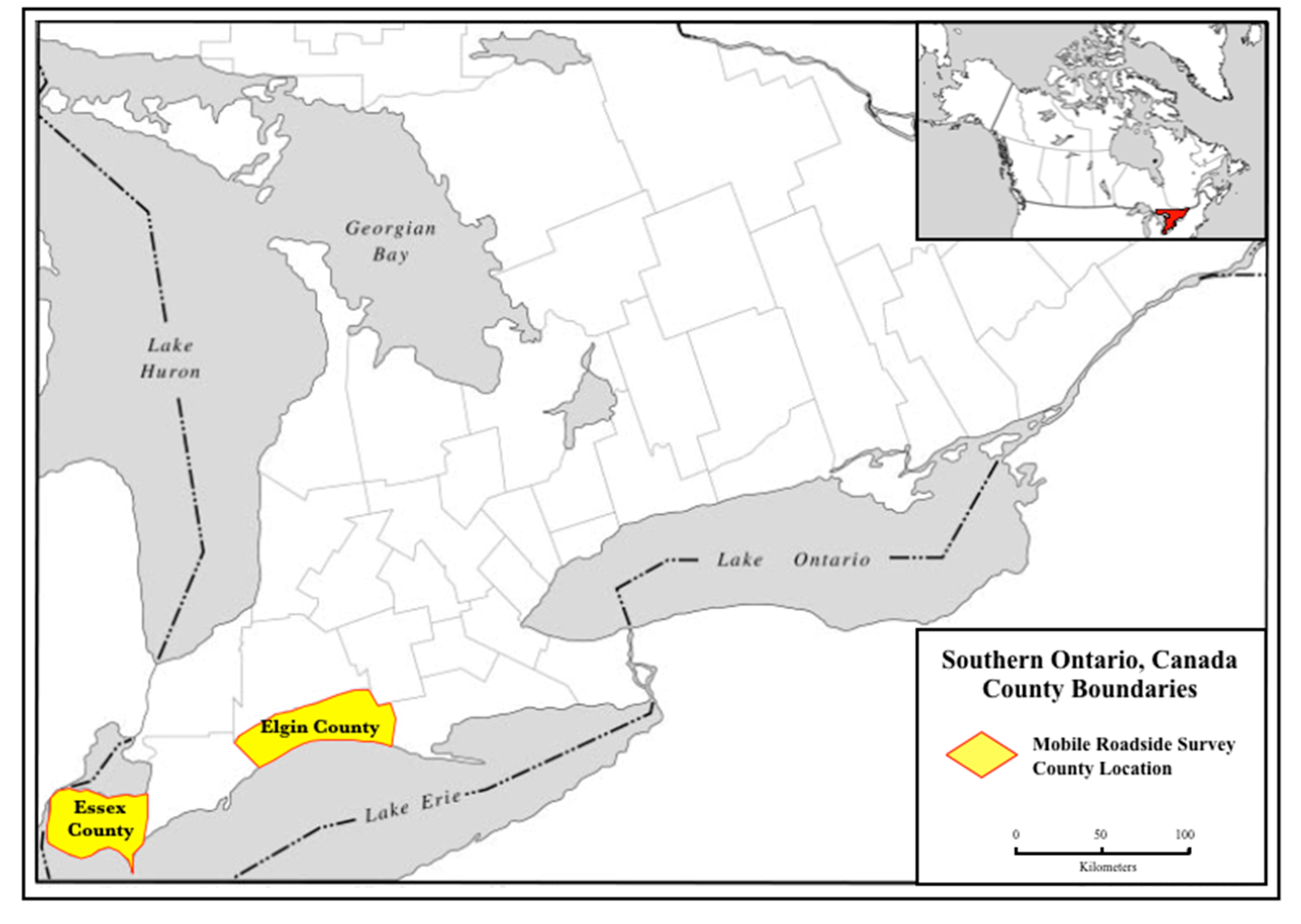
Fieldwork was conducted in Elgin and Essex counties in southwestern Ontario, Canada (Figure 1). Dominant crops in these areas include corn (Zea mays), soybean (Glycine max), and winter wheat (Triticum aestivum L.) often grown in rotation, interspersed occasionally with perennial forages. As discussed above, various practices are followed after harvest, including use of CV, CS, NT, or GC, resulting in different soil surface cover conditions during the non-growing season.
2.2. Instrumentation Description
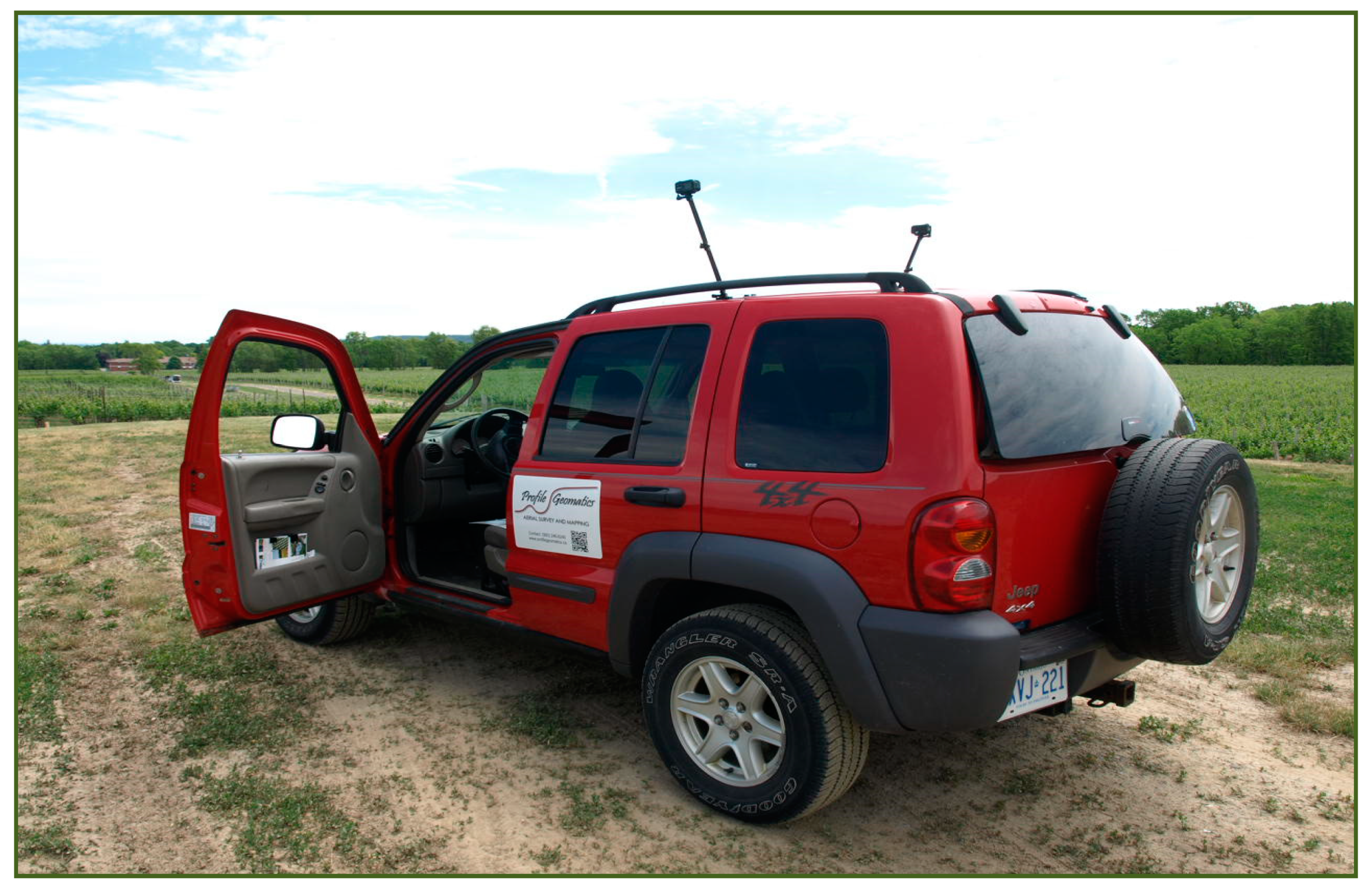
The vehicle mounted roadside imagery system (Figure 2) included a pair of GPS enabled Garmin VIRB XE 12 MP digital imaging cameras with auto exposure (generally running between 1/1000 and 1/2500 of a second) and variable aperture settings automatically calculated based on incident illumination. Various camera systems could be employed in such a system (e.g., GoPro) however the features of the selected cameras that made it suitable for this experiment included: the variable aperture settings to allow the cameras to capture suitable photos under variable lighting conditions such as intermittent clouds (pictured in Figure 2); a built in GPS to geolocate the photo locations; wide angle footage with electronic image stabilization (based on built-in accelerometers) to reduce blurring effects from camera vibration; Wi-Fi capability to allow for remote camera operation and previewing images from a tablet within the vehicle; and waterproof cases. The two cameras were mounted perpendicular to the vehicle’s direction of travel, extended above permanent mounting brackets to an above ground elevation of 2.3m on the right (curb-side) and 2.6m on the left (driver-side) to compensate for the additional distance to the fields. The extension poles were further reinforced against vibration using foam insulated cable ties to roof rails and support mounts on the vehicle. A large proportion of the driving route for each county was comprised of rough gravel, or packed dirt roads; hence, a 4WD with a modified soft suspension was required to reduce vibration on the imaging platforms themselves. Further, the 4WD vehicle, with its higher ground clearance, allowed for higher mounting of the side-looking cameras.
2.3. Data Collection and Processing
Data collection for Essex and Elgin County were carried out on May 18 and 20, 2016, respectively. The Essex County survey had a total driving distance of 102 km and the Elgin County survey a total driving distance of 248 km. Atmospheric conditions for both dateswere mostly clear. Although not examined directly in this paper, the acquisition of the roadside images was conducted to coincide with a Landsat 8 OLI overpass and was collected concurrent with in-field ground-truth data collection for each respective area [4]. Data collection was carried out in this manner to produce a value-added product that could be employed for ground-truth evaluation of future studies employing the Landsat orbital platform.
Route maps (shown partially in Figure 3) were designed for the two sampling locations to minimize overlap in image acquisition, and to ensure adequate coverage of manually sampled field plots for comparison between mobile collected, and in-field static image capture and residue quantification. Overlap of the roadside photos was not of interest for this study, as only one or two photos were needed to characterize post-harvest land cover over each field. The driving speed was maintained between 40–45 km/h to ensure image capture of every field, with shutter actuation on each camera set at 5-second intervals. Reduced driving speeds were also required to reduce camera vibration.
To ensure that each field was adequately imaged, the shutter actuation (SA) was predetermined before each trip. The SA was determined by dividing the proposed upper limit of the driving speed (m/s) by the number of images to appropriately image each field, given a predetermined estimate of the typical field size in each county. Multiple field image captures (≈2–3 images per field) was conducted in the event that undesired features (e.g. people, vehicles, trees, etc.) were visible at the forefront of the imaging plane, obscuring the background.
Following image collection in each county, the photos were transferred to a desktop computer for sorting. A total of 18,462 images were acquired for the 2 routes/days. The images were sorted by site, date, and look direction for the particular camera. The clearest, most central image of the field (from the 2–3 captured) was retained. Images not meeting the requirements of the project were subsequently deleted, resulting in a filtered dataset containing imagery for 991 and 772 agricultural fields in Elgin and Essex County, respectively. This manual sorting was the longest aspect of the research, requiring approximately 1 full day to visually inspect and delete non useful photographs. Examples of deleted scenes include images of forests, houses, quarries, intersections, overpasses, non-agricultural structures, road-vehicles, or any that contained identifiable footage of individuals.
An issue prevalent with wide-angle oblique image capture is the so-called fisheye, or barrel, effect. The geometric distortion in the radial direction, present in all aspects away from the centroid of the imaging plane, results from compression in peripheral regions, allowing for a wide-angle view to be presented in the image plane [27]. Such distortion presents issues in many land-use studies by virtue of a variable pixel-to-ground scale across the image plane, and the removal of lens distortion is preferred in multi-class image classification, especially where volumetric measures of scene features are required [26,28]. Image correction was performed using software from Liquivid© Video Fisheye Removal. The correction permits cross platform image sharing where geometrically rectified imagery is required.
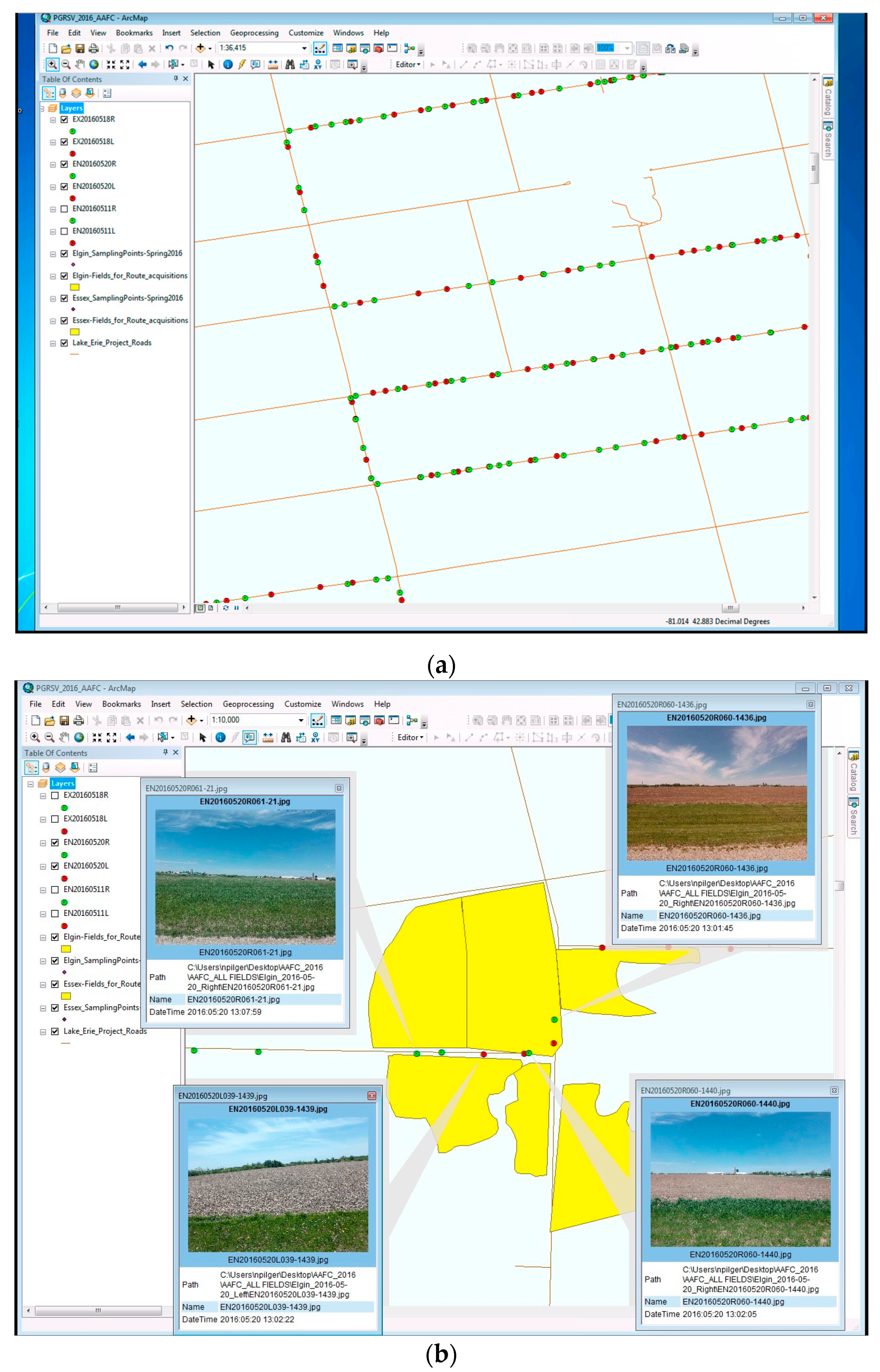
The GPS vehicle mounted cameras included the horizontal geographic latitude and longitude coordinate information, in addition to other variables including elevation, slope, and aspect, that are transferrable to the imagery via still-to-video image conversion. The transfer of ancillary information to coordinate geometry was performed by creating a stop-motion video comprised of the 4 sorted, and geometrically rectified image data-sets (left and right look direction for 2 acquisitions), and then deconstructing the video back to individual static images. The process allowed for extraction of coordinate coding for each image and the generation of a point for each image location to be displayed in a Geographic Information System (GIS) (Figure 3a).
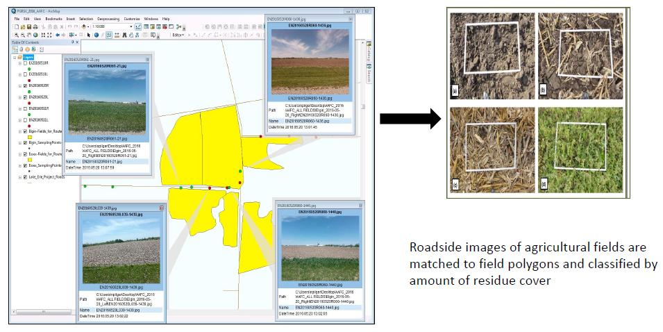
A geodatabase of the roadside imagery was created within an ESRI ArcGIS 10.1 environment, with the polygons of the individual agricultural fields digitized from air photos. The roadside images were linked to a point feature class layer for spatial identification based on the inherent coordinate data captured coincident with the roadside imagery (Figure 3b). Each camera had a dedicated micro-SD card for storage of photos from the driver and passenger side of the vehicle. The vehicle direction and orientation were determined using the photo time stamps. The point feature classes (photos) were then linked to the appropriate field polygons (based on vehicle orientation) to allow for photo identification with each field in the study region. This procedure allows the user to zoom in to each field location and visually assess any roadside images connected to the given field polygon (Figure 3b).
Storage of the photos within a GIS allows for updating the imagery related to each field and would facilitate comparison of tillage practices to establish a land cover time series. The sorted images were individually assessed by personnel trained in conducting visual roadside surveys to classify fields to one of four residue classes (described in the introduction and shown in Figure 4). The green cover class was assigned when >90% field was visually composed of green, actively photosynthesizing vegetation. For this experiment, the classification of the oblique roadside images was carried out by 4 individually trained researchers, and subsequently recorded on a spreadsheet for each field. The independent classifications were then combined, and final labeling based on simple majority rule applied (no ties occurred). Automated methods, such as those described in [29], could be implemented. However, these approaches are typically not applied to the oblique camera views used in this study.
2.4. Image Validation
Validation of the residue land cover classes (Figure 4) estimated from the roadside image capture system was performed using data from 114 research sites across the two counties. This field data was obtained either the same day or within one day of the roadside image capture. The in-field research sites were evaluated for soil cover using a photo-grid sampling technique where average counts were derived from three digital images captured at 90 degrees from surface normal, or nadir view, using 0.75 × 1.0 m survey quadrats over a 30 m × 30 m area; the three photo locations were selected to represent the low, medium, and high range of soil cover in the field [29]. Residue and green cover counts of the quadrat photos were performed using 10 × 10 digital grids, representing 100 points for each photo imaging frame (e.g., left side of Figure 4 [3,4,29], where cover percentage was based on presence or absence over each of the 100 grid intersection points, and categorized as CV (0%–30%); CS (30–60%); and NT (60%–100%). For this experiment, the green cover class was assigned when >90% field was visually composed of green, actively photosynthesizing vegetation which was representative of the spring season (May); however, different classifications of green cover may be desired if the survey was conducted in the fall when green cover would be less established. The nadir photo-grid counts were conducted by different technicians than those assessing roadside oblique images visually to reduce bias. The three photo-based residue measures taken on each field were averaged for each of 114 field sites, resulting in an estimate of the percentage of cover for each site. This digital method of in-field residue evaluation was found to be highly correlated to traditional line transect methods to accurately estimate post-harvest residue percentages, but in a more efficient manner [3]. The fields where the samples were taken were typically large (>40 ha) with relatively homogeneous land management practices employed, therefore the photos taken from both the vehicle system and nadir within the field are assumed to be representative of the overall landcover within the field. Residue coverage may not be homogeneous in the field, this often occurs near the field edge, therefore, the in-field sample sites were at least 100 m from any field boundary, and the assessment of the roadside photos was for mid-field residue conditions as much as possible.
3. Results
A confusion matrix (shown in Table 1) was used to compare classes based on imagery captured by the mobile roadside sytem against coincident in-field collected data classes for the 114 research sites distributed over the two counties surveyed during this pilot project. While overall agreement between mobile roadside (MR) collected imagery and in-field (IF) classification was strong, there are some minor areas of confusion, primarily between conservation (CS) and no-till (NT) fields. This may be explained by the visual similarity at distance from the roadside between these two land-classes (Figure 4b,c (right side)). In particular the oblique camera view may overestimate the cover in the case of standing residue. However, overall accuracy of the approach was 93% and the calculated Kappa Coefficient of Agreement was 0.904 suggesting very strong agreement [30].
Another issue relating to confusion between the tillage classes involves the look direction variation between nadir and oblique image capture. For example, a harvested field of corn will appear to contain higher levels of residue in an oblique image, as we are viewing the residue from the side, and overlap occurs as a function of perspective, whereas in a nadir view a greater proportion of bare soil will be visible within the image.
Using the described approach, a total of 772 fields were mapped within Essex County, and 991 fields in Elgin County. The results of the survey are characterized in Table 2. Over both counties’, CV practices dominate the fields imaged, accounting for approximately 1/3 or greater of land management practices. This is not an unusually high level, given that the imaging took place past mid-May, when planting of corn had already taken place and soybean planting was still underway in these counties, which could have influenced conventional land cover rates as spring tillage and planting implements can breakdown and bury previous crop residue. Combined, conservation and no-till practices are conducted more within Essex County (≈36% of fields mapped) than observed in Elgin County (29%). As both Conservation tillage and No-Till meet thresholds that are representative of conservation methods (i.e., >30% cover for soil erosion protection), the misclassification demonstrated in Table 1 between these two classes would be acceptable in this case. The roadside survey was also able to identify land management practices that did not fit into the classification scheme. These activities include permanent pasture, orchards, and sod farms. Several of these activities could be susceptible to misclassification errors when using moderate resolution remote sensing products without using further verification data, such as annual crop survey information [21] or the images available from the roadside survey.
4. Discussion
The key benefit of the described mobile roadside reference data collection method was the flexibility of not relying on specific meteorological conditions coinciding with satellite pass dates, as is the case with most optical airborne and orbital platforms. Other potential advantages included: enhanced safety by eliminating roadside pullover for manual real-time roadside classification, reduction of driver distraction by incorporating an automatic imaging system, and creation of archival footage of land cover conditions for future reference or for corroboration with satellite-based surveys. In southwestern Ontario, skies are often overcast during the non-growing season (particularly in autumn), limiting traditional classification using orbital, or high-altitude airborne image capture. With the described mobile system, specific fields that have not been harvested at the time of roadside image capture may readily be re-visited, or field-data may be in-filled at a later date, either via direct contact with land holders, or through other citizen provided reference data [31].
Mounted with opposing side viewing cameras, the roadside survey vehicle was shown to be highly efficient in the collection of geo-referenced imagery of up to 500 fields per hour, with an overall level of agreement to in-field ground surveys at 93 percent, employing a single vehicle and a single operator to produce a more reliable and robust data-set for extrapolation to larger areas. As shown in Table 1, errors are typically limited to distinctions between the conservation and no-till classifications. Hively et al. [32] conducted a similar study that verified residue coverage using optical satellite data with information from roadside surveys. They noted the largest discrepancies between the classified satellite images and the roadside surveys satellite occurred at moderate residue classes and suggest that the oblique angles of the survey may contribute to this impact. Inspection of classification errors for our data set suggests that the roadside image approach overestimates relative to the nadir photos. In particular, our errors in the classification occurred near the thresholds (e.g., 30% for CV vs. CS or 60% for CS vs. NT), with the roadside images biased towards more residue. As we manually classified the roadside photos into the main residue classes, a direct 1:1 relationship between the nadir and roadside images could not be completed, however, the direction of the bias (in this case bias towards more residue near the thresholds) should be noted.
With respect to efficiency, the post processing of the nadir infield photos and of the roadside images are similar in the amount of the time required for laboratory processing (i.e., sorting, counting, and classification) after acquisition of the photos. As traditional measures extrapolate a small sample over larger areas, a census method described here potentially minimizes error promoted through bias in the sampling methodology, by surveying a much greater number of fields over a larger geographic extent while simultaneously providing a robust data record, not dependent on meteorological conditions. We also believe the cost of the data collection is significantly lower than low-altitude aerial image capture (assuming the costs of the rental of an aircraft or the large number of UAVs necessary to conduct a similar sized survey of more than1000 fields surveyed in two days). With respect to UAVs, their use is limited to line of site in our study region, which would further limit their use for the broad areas covered over a short time discussed here. Another benefit is that time series of these vehicle mounted camera surveys would permit change detection analysis over subsequent anniversary dates, regardless of atmospheric conditions, to quickly assess how land owners are adapting land management practice to climate and weather, to monitor the land use implications of changes to regulations toward the adoption of particular cropping practices, and to perform more routine measurement of soil cover [33,34].
The roadside survey techniques described will have value for further interpretation in follow up satellite derived residue and cover crop validation studies e.g., [4,32]. In residue quantification studies such as [2,4], where selection of both high and low residue endmembers was necessary for the development of spectral unmixing components, the ability to corroborate the selection process with a large number of near coincident photos would be beneficial. The corroboration can also be useful for verification. For example, based on the date of our captured images, some fields showed evidence of very recent soil turning; therefore, the fields analyzed may indicate higher levels of soil disturbance being classed as conventional tillage, than what may in fact be a conservation practice carried out over the majority of the non-growing season by the landowner (with only recent seedbed preparation). In this respect, one must take into account the temporal influence of any tillage residue survey. With many agricultural surveys being carried out coincident with satellite overpass, these rapid transitions may result in potential classification errors, thus reinforcing the benefit of complementary non-orbital dependent classification techniques.
There are challenges that should be noted for researchers interested in developing similar systems. Notably:
- Driving speed: Higher speeds could lead to blurring effects in lower light conditions, particularly closer to the lens. However, preliminary comparative tests between images captured at 40 km/h in bright atmospheric conditions and images captured at 60 km/h during overcast conditions were similar in quality.
- Wind speed: As with vehicular velocity above, higher wind speeds increase vibration through the vehicle and the extended camera mounts. Vibration can significantly affect image clarity and subsequent assessments. From this pilot project, there was some evidence that heavy gusts offset the horizontal plane of the camera.
- Shutter actuation: Shutter actuation, is intrinsically linked to driving speed and external light conditions. The cameras could technically achieve 10 shots/s. However, the associated image sorting time would be inefficient. Therefore, using knowledge of field size and proposed driving speed to ensure that the shutter actuation results in a minimum of three images per field can reduce post-processing time associated with sorting of the photos.
- Privacy concerns: Privacy concerns are paramount in post-production, though not a technical issue. Any images where people, especially children, vehicles, homes, etc., are visible and identifiable, have potential to raise privacy concerns depending on local laws. With a sound editing and sorting methodology, any such images can be deleted in an expedient manner.
5. Conclusions
Agricultural land cover management practices have impact on soil health through retaining plant residues and water quality, through reduction of overland flow and subsequent soil erosion and transport to water courses. Knowledge of land cover practices is thus a necessary input for many erosion modeling tools, yet over large areas, this data is often not available. Several satellite remote sensing techniques have been developed for characterization of land management practices, but these approaches are typically dependent on clear atmospheric conditions at the time of overpass. Furthermore, many of these approaches still require ground verification data [2,4,32]. To broadly survey practices over large regions, methods for timely collection of land management data are necessary. This project has demonstrated that a semi-automated, vehicular approach for rapid collection and determination of post-harvest tillage and green cover practices has relatively high accuracy (overall accuracy 93%; Kappa agreement 0.904), compared to nadir validation photos, for characterization of the four non-growing season land cover classifications used in Ontario Canada (CV, CS, NT, and green cover). Based on this result we suggest that the approach would be beneficial for conducting land cover surveys when atmospheric conditions are unfavorable for satellite remote sensing, or for collecting census level data for validation and error estimation of remotely sensed estimates.
Author Contributions
Conceptualization, N.P. and A.B.; Data curation, N.P. and P.J., Formal analysis, N.P., A.B., and P.J. Funding acquisition, A.B. and P.J.; Methodology, A.B. and N.P.; Writing—original draft, N.P. and A.B. Writing—review & editing of original draft, N.P., A.B., and P.J. All authors have read and agreed to the published version of the manuscript.
Funding
This research was funded by the Ontario Ministry of Agriculture Food and Rural Affairs and Agriculture and Agri-food Canada. The views expressed in this publication are those of the authors and do not necessarily reflect those of the Province of Ontario or the Government of Canada. Additional funding was provided Canada First Research Excellence Fund—Food from Thought.
Acknowledgments
Joshua Antinolfi and Garrett Mellan are acknowledged for their role in the interpretation of the field photos. Thanks to Jennifer Birchmore and Adam Hayes Ontario Ministry of Agriculture, Food and Rural Affairs for their sharing of manual roadside survey protocols and training materials, and Ahmed Laamrani and Natalie Feisthauer from Agriculture and Agri-Food Canada STB Guelph for supporting in-field photo data collection and analysis.
Conflicts of Interest
The authors declare no conflict of interest.
Disclaimer
The use, evaluation, and reference to particular products by the authors of this manuscript should not be regarded as an endorsement by AAFC or the University of Guelph.
References
- Hussain, M.; Chen, D.; Cheng, A.; Wei, H.; Stanley, D. Change detection from remotely sensed images: From pixel-based to object-based approaches. ISPRS J. Photogram Remote Sens. 2013, 80, 91–106. [Google Scholar] [CrossRef]
- Pacheco, A.; McNairn, H. Evaluating multispectral remote sensing and spectral unmixing analysis for crop residue mapping. Remote Sens. Environ. 2010, 114, 2219–2228. [Google Scholar] [CrossRef]
- Laamrani, A.; Joosse, P.; Feisthauer, N. Determining the number of measurements required to estimate crop residue cover by different methods. J. Soil Water Conserv. 2017, 72, 471–479. [Google Scholar] [CrossRef] [Green Version]
- Laamrani, A.; Joosse, P.; McNairn, H.; Berg, A.A.; Hagerman, J.; Powell, K.; Berry, M. Assessing soil cover levels during the Non-Growing Season Using Multitemporal Satellite Imagery and Spectral Unmixing Techniques. Remote Sens. 2020, 12, 1397. [Google Scholar] [CrossRef]
- Daughtry, C.S.T.; Doraiswamy, P.C.; Hunt, E.R.; Stern, A.J.; McMurtrey, J.E.; Prueger, J.H. Remote sensing of crop residue cover and soil tillage intensity. Soil Tillage Res. 2006, 91, 101–108. [Google Scholar] [CrossRef]
- Moreira, W.H.; Tormena, C.A.; Karlen, D.L.; da Silva, A.P.; Keller, T.; Betioli, E., Jr. Seasonal changes in soil physical properties under long-term no-tillage. Soil Tillage Res. 2016, 160, 53–64. [Google Scholar] [CrossRef] [Green Version]
- Dam, R.F.; Mehdi, B.B.; Burgess, M.S.E.; Madramootoo, C.A.; Mehuys, G.R.; Callum, I.R. Soil bulk density and crop yield under eleven consecutive years of corn with different tillage and residue practices in a sandy loam soil in Central Canada. Soil Tillage Res. 2005, 84, 41–53. [Google Scholar] [CrossRef]
- West, T.O.; Post, W.M. Soil organic carbon sequestration rates by tillage and crop rotation. Soil Sci. Soc. Am. J. 2002, 66, 1930–1946. [Google Scholar] [CrossRef] [Green Version]
- Laamrani, A.; Voroney, P.R.; Berg, A.A.; Gillespie, A.; March, M.; Deen, B.; Martin, R.C. Temporal change of soil carbon on a long-term experimental site with variable crop rotations and tillage systems. Agronomy 2020, 10, 840. [Google Scholar] [CrossRef]
- Mathew, R.P.; Feng, Y.; Githinji, L.; Ankumah, R.; Balkcom, S.K. Impact of No-Tillage and Conventional Tillage Systems on Soil Microbial Communities. Appl. Environ. Soil Sci. 2012. [Google Scholar] [CrossRef] [Green Version]
- Govaerts, B.; Mezzalama, M.; Unno, Y.; Sayre, K.D.; Luna-Guido, M.; Vanherck, K.; Dendooven, L.; Deckers, J. Influence of tillage, residue management, and crop rotation on soil microbial biomass and catabolic diversity. Appl. Soil Ecol. 2007, 37, 18–30. [Google Scholar] [CrossRef]
- Spedding, T.A.; Hamel, C.; Mehuys, G.R.; Madramootoo, C.A. Soil microbial dynamics in maize-growing soil under different tillage and residue management systems. Soil Biol. Biochem. 2004, 36, 499–512. [Google Scholar] [CrossRef]
- Blanco-Canqui, H.; Wienhold, B.J.; Jin, V.L.; Schwer, M.R.; Kibet, L. Long-term tillage impact on soil hydraulic properties. Soil Tillage Res. 2017, 170, 38–42. [Google Scholar] [CrossRef] [Green Version]
- Manns, H.R.; Berg, A.A.; Bullock, P.R.; McNairn, H. Impact of soil surface characteristics on soil water content variability in agricultural fields. Hydrol. Process. 2014, 28, 4340–4351. [Google Scholar] [CrossRef]
- Dolan, M.S.; Clapp, C.E.; Allmaras, R.R.; Baker, J.M.; Molina, J.A.E. Soil organic carbon and nitrogen in a Minnesota soil as related to tillage, residue and nitrogen management. Soil Tillage Res. 2006, 89, 221–231. [Google Scholar] [CrossRef]
- Halvorson, A.; Wienhold, B.J.; Black, A.L. Tillage, Nitrogen, and Cropping System Effects on Soil Carbon Sequestration. Soil Sci. Soc. Am. J. 2002, 66, 906–912. [Google Scholar] [CrossRef]
- Angers, D.A.; Bolinder, M.A.; Carter, M.R.; Gregorich, E.G.; Drury, C.F.; Liang, B.C.; Voroney, R.P.; Simard, R.R.; Donald, R.G.; Beyaert, R.P.; et al. Impact of tillage practices on organic carbon and nitrogen storage in cool, humid soils of eastern Canada. Soil Tillage Res. 1997, 41, 191–201. [Google Scholar] [CrossRef]
- Jabro, J.D.; Iversen, W.M.; Stevens, W.B.; Evans, R.G.; Mikha, M.M.; Allen, B.L. Physical and hydraulic properties of a sandy loam soil under zero, shallow and deep tillage practices. Soil Tillage Res. 2016, 159, 67–72. [Google Scholar] [CrossRef]
- Arshad, M.A.; Franzluebbers, A.J.; Azooz, R.H. Components of surface soil structure under conventional and no-tillage in northwestern Canada. Soil Tillage Res. 1999, 53, 41–47. [Google Scholar] [CrossRef]
- Derpsch, R. Conservation Tillage, No-Tillage and Related Technologies. In Conservation Agriculture; Garcia-Torres, L., Benites, J., Martinez-Viela, A., Holgado-Cabrera, A., Eds.; Springer: Dordrecht, The Netherlands, 2003. [Google Scholar]
- Davidson, A.M.; Fisette, T.; McNairn, H.; Daneshfar, B. Detailed crop mapping using remote sensing data (Crop data layers) (Chapter 4). In Handbook on Remote Sensing for Agricultural Statistics; Delince, J., Ed.; Handbook of the Global Strategy to Improve Agricultural and Rural Statistics; GSARS: Rome, Italy, 2017; pp. 91–129. [Google Scholar]
- Thoma, D.P.; Gupta, S.C.; Bauer, M.E. Evaluation of optical remote sensing models for crop residue cover assessment. J. Soil Water Conserv. 2004, 59, 224–233. [Google Scholar]
- McNairn, H.; Brisco, B. The application of C-band polarimetric SAR for agriculture: A review. Can. J. Remote Sens. 2004, 30, 525–542. [Google Scholar] [CrossRef]
- Adams, J.R.; Berg, A.A.; McNairn, H.; Merzouki, A. Sensitivity of C-band SAR polarimetric variables to unvegetated agricultural fields. Can. J. Remote Sens. 2013, 39, 1–6. [Google Scholar] [CrossRef]
- Remondino, F.; Gerke, M. Oblique Aerial Imagery—A Review. In Photogrammetric Week 2015; Fritsch, D., Ed.; Wichmann/VDE Verlag: Belin/Offenbach, Germany, 2015; pp. 75–83. [Google Scholar]
- Stockdale, C.A.; Bozzini, C.; Macdonald, S.E.; Higgs, E. Extracting ecological information from oblique angle terrestrial landscape photographs: Performance evaluation of the WSL Monoplotting Tool. Appl. Geogr. 2015, 63, 315–325. [Google Scholar] [CrossRef]
- Kim, D.; Paik, J. Three-dimensional simulation method of fish-eye lens distortion for a vehicle backup rear-view camera. J. Optical Soc. Am. 2015, 32, 1337–1343. [Google Scholar] [CrossRef] [PubMed]
- Chow, J.C.K.; Detchev, I.; Ang, K.D.; Morin, K.; Mahadevan, K.; Louie, N. Robot Vision—Calibration of wide-angle lens cameras using collinearity Condition and K-Nearest Neighbor Regression. Ecol. Econ. 2018, 111, 93–99. [Google Scholar]
- Laamrani, A.; Pardo Lara, R.; Berg, A.A.; Branson, D.; Joosse, P. Using a Mobile Device “App” and Proximal Remote Sensing Technologies to Assess Soil Cover Fractions on Agricultural Fields. Sensors 2018, 18, 708. [Google Scholar] [CrossRef] [Green Version]
- Congalton, R.G.; Green, R.A. Assessing the Accuracy of Remotely Sensed Data: Principles and Practices, 2nd ed.; CRC Press: Boca Raton, FL, USA, 2009; p. 183. [Google Scholar]
- Foody, G.M. An assessment of citizen contributed ground reference data for land cover map accuracy assessment. Proc. ISPRS Ann. Photogramm. Remote Sens. Spat. Sci. 2015, 219–225. [Google Scholar] [CrossRef] [Green Version]
- Hively, W.D.; Shermeyer, J.; Lamb, B.T.; Daughtry, C.T.; Quemada, M.; Keppler, J. Mapping crop residue by combining Landsat and WorldView-3 satellite imagery. Remote Sens. 2019, 11, 1857. [Google Scholar] [CrossRef] [Green Version]
- Kennedy, R.E.; Townsend, P.A.; Gross, J.E.; Cohen, W.B.; Bolstad, P.; Wang, Y.Q.; Adams, P. Remote sensing change detection tools for natural resource managers: Understanding concepts and tradeoffs in the design of landscape monitoring projects. Remote Sens. Environ. 2009, 113, 1382–1396. [Google Scholar] [CrossRef]
- Vercammen, J. Agri-Environmental Regulations, Policies, and Programs. Can. J. Agric. Econ. 2011, 59, 1–18. [Google Scholar] [CrossRef]
Figure 1.
Map of Ontario counties where the roadside surveys were conducted.

Figure 2.
Roadside survey vehicle camera system with roof-top camera mounts.

Figure 3.
Examples of the georeferenced roadside survey. (a) illustrates roadside survey locations, with green points showing photos taken from right side of the vehicle (driving direction), and red from the left. Vehicle driving directions can be determined from the embedded time stamps in the photos. (b) illustrates examples of the photos acquired for the polygons of the sampled agricultural fields.

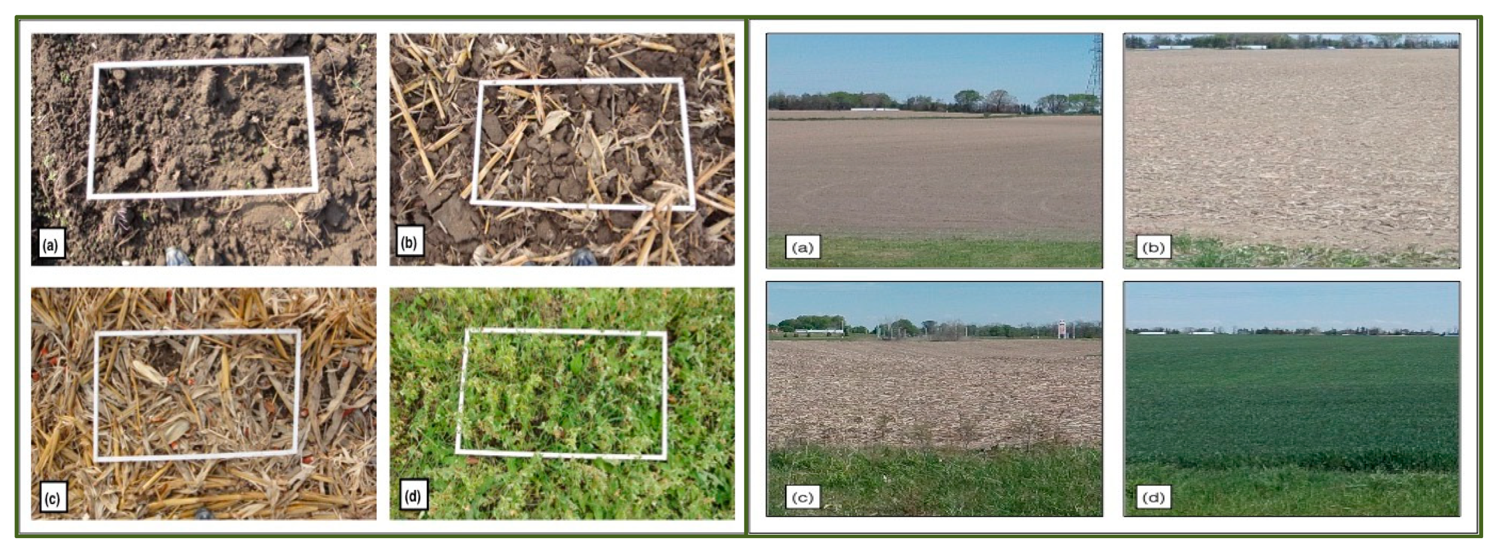
Figure 4.
Non-growing season soil cover classifications shown from nadir (left) and oblique (right) vantage points. (a) illustrates conventional tillage practices with little visible residue (CV); (b) illustrates conservation tillage (CS) practices (≈30–60% residue); (c) presents no-till (NT) practices with greater than 60% residue; (d) illustrates green cover (GC) classification.


Table 1.
Error matrix mobile roadside (MR) oblique vs. ground collected nadir in-field (IF) imagery, for conventional tillage (CV); conservation tillage (CS); no-till (NT); and green cover (GC) practices. Validation was carried out over 114 field sites in Elgin and Essex County. Omission and Commission error values for each land class are reported in the last row and column, respectively, with an overall accuracy (OA) of 93%.
| Categories | IF-CV | IF-CS | IF-NT | IF-GC | Commission Error |
|---|---|---|---|---|---|
| MR-CV | 30 | 1 | 0 | 0 | 31 (3.2%) |
| MR-CS | 0 | 21 | 5 | 0 | 26 (19.2%) |
| MR-NT | 0 | 2 | 37 | 0 | 39 (5.1%) |
| MR-GC | 0 | 0 | 0 | 18 | 18 (0%) |
| Total | 30 | 24 | 42 | 18 | |
| Omission Error | 0% | 12.5% | 11.9% | 0% | OA = 93% |
Table 2.
Results of the agricultural land management classification survey over Essex and Elgin counties on 18–20 May 2016 respectively. An “other” class was added to denote agricultural activities that were not definable by tillage and green cover management practices, including land uses such as pastures and orchards.
| Essex County | Elgin County | |
|---|---|---|
| CV | 31.8% | 38.9% |
| CS | 22.4% | 21.1% |
| NT | 13.8% | 8.5% |
| GC | 18.1% | 25.7% |
| Other | 13.7% | 5.8% |
| Total | 772 | 991 |
© 2020 by Her Majesty the Queen in Right of Canada as represented by the Minister of Agriculture and Agri-Food and © 2020 by authors Pilger and Berg. Submitted for possible open access publication under the terms and conditions of the Creative Commons Attribution (CC BY) license (http://creativecommons.org/licenses/by/4.0/).
Share and Cite
MDPI and ACS Style
Pilger, N.; Berg, A.; Joosse, P. Semi-Automated Roadside Image Data Collection for Characterization of Agricultural Land Management Practices. Remote Sens. 2020, 12, 2342. https://0-doi-org.brum.beds.ac.uk/10.3390/rs12142342
AMA Style
Pilger N, Berg A, Joosse P. Semi-Automated Roadside Image Data Collection for Characterization of Agricultural Land Management Practices. Remote Sensing. 2020; 12(14):2342. https://0-doi-org.brum.beds.ac.uk/10.3390/rs12142342
Chicago/Turabian StylePilger, Neal, Aaron Berg, and Pamela Joosse. 2020. "Semi-Automated Roadside Image Data Collection for Characterization of Agricultural Land Management Practices" Remote Sensing 12, no. 14: 2342. https://0-doi-org.brum.beds.ac.uk/10.3390/rs12142342
Note that from the first issue of 2016, this journal uses article numbers instead of page numbers. See further details here.