Assessment of Tree Detection Methods in Multispectral Aerial Images


1
CONACYT, CIIDIR Oaxaca, Instituto Politécnico Nacional, 71230 Oaxaca, Mexico
2
Department of Forest Ecosystems & Society, Oregon State University, Corvallis, OR 97331, USA
3
Massachusetts Institute of Technology, Cambridge, MA 02139, USA
*
Author to whom correspondence should be addressed.
Remote Sens. 2020, 12(15), 2379; https://0-doi-org.brum.beds.ac.uk/10.3390/rs12152379
Submission received: 15 June 2020
/
Revised: 11 July 2020
/
Accepted: 14 July 2020
/
Published: 24 July 2020
(This article belongs to the Special Issue Individual Tree Detection and Characterisation from UAV Data)
Abstract
:Detecting individual trees and quantifying their biomass is crucial for carbon accounting procedures at the stand, landscape, and national levels. A significant challenge for many organizations is the amount of effort necessary to document carbon storage levels, especially in terms of human labor. To advance towards the goal of efficiently assessing the carbon content of forest, we evaluate methods to detect trees from high-resolution images taken from unoccupied aerial systems (UAS). In the process, we introduce the Digital Elevated Vegetation Model (DEVM), a representation that combines multispectral images, digital surface models, and digital terrain models. We show that the DEVM facilitates the development of refined synthetic data to detect individual trees using deep learning-based approaches. We carried out experiments in two tree fields located in different countries. Simultaneously, we perform comparisons among an array of classical and deep learning-based methods highlighting the precision and reliability of the DEVM.
1. Introduction
Programs to reduce emissions from deforestation and forest degradation (e.g., REDD+ [1]) intend to mitigate the effects of climate change by providing forest landowners with economic incentives reflecting the value of the carbon stored within the trees. However, despite advancements in remote sensing technology, manual labor still needs to accomplish many measurements, such as estimating the overall vegetation biomass and the carbon stored in individual trees and forests. For example, it is common for field crews to travel to inventory plots and perform tasks such as counting and measuring tree sizes using visual estimations and manual measurements. This approach requires a considerable amount of time and resources, e.g., the USDA Forest Service spends more than 75% of the inventory costs on data collection [2].
This study describes methodologies that efficiently detect trees automatically using remote sensing technology (see Figure 1). In our approach, we collected data using unoccupied aerial systems (UAS) equipped with multispectral cameras sensitive to the green, red, red edge, and near-infrared wavelengths. Using structure from motion techniques (SfM) [3], we obtained 4-band orthophotos, digital surface models (DSM), and digital terrain models (DTM) [4] in the form of orthomosaics. Then, we calculated the Normalized Difference Vegetation Index (NDVI) [5] from the multispectral orthophotos. After the orthophotos registration, we utilized the DSM, DTM, and NDVI to obtain a Digital Elevated Vegetation Model (DEVM). We then generated a synthetic data set of DEVM images that we used to train classic and modern machine learning algorithms to detect trees. Finally, performance tests using two tree plots in different countries indicated the precision of the new method. Our results show that Convolutional Neural Network (CNN)-based methods have become the leading performer. Nonetheless, classic approaches remain competitive and may offer advantages in settings where data collection and available computing resources for training are an issue.
Our main contributions include:
- The introduction of the DEVM, an image representation that blends aboveground structural information and quantification of vegetation suitable for the detection of trees;
- the development of a scheme to generate synthetic data sets of trees in DEVM space for training classical and modern tree detection methods;
- the assessment of classical and modern techniques, trained with synthetic images, to detect treetops.
We structure the rest of the document as follows. In the next section, we describe the current state-of-the-art and practice regarding tree detection. Then, in Section 3, we formulate the foundation of the newly developed DEVM, provide further detail about the method to generate synthetic tree data sets, and detail the classical and modern techniques we benchmark in the paper. In Section 4, we describe the effects of implementing the methods to detect treetops in two tree plots and compare their performance. We continue the paper discussing our results in Section 5 and finally conclude summarizing our findings and delineating possible directions for future research.
2. Related Literature
This section reviews the scientific literature describing classical and modern approaches for tree detection with particular emphasis on aerial images. In addition, related to our work, we discuss the research aiming to generate synthetic images for training deep learning methods and describe the image sources for automatic tree detection.
2.1. Classical Tree Detection
Classical methods for detecting trees rely mostly on crafted features (see [6,7,8] for reviews of approaches to detect individual tree crowns). The proposed methods include local maxima filtering, template matching, valley following, watershed region growing, circular structures fitting, and Support Vector Machines with Histograms of Oriented Gradients (HOG) features. Some recent research follows this trend. For instance, basing tree’s detection on edge votes required applying tree crown delineation for the candidates using watershed segmentation (Özcan et al. [9,10]). The eccentricity of the ellipses to fit these segments was used to discard human-made objects. Another method filtered out non-vegetation utilizing NDVI (Ozdarici-Ok [6]). The selection of tree crows employed the gradient to detect high radial symmetry and increased diameter thresholds. A third method was based on the binarization of RGB images (Reza et al. [11]). An adaptive median filter removed noise and distortion before a morphological operation outlined the boundaries between the plants.
Alternatively, Maillard and Gomes [12], and Bao et al. [13] used template matching to detect trees. The former detects deciduous trees using a geometrical–optical model as a template, which includes parameters such as illumination angles, maximum and ambient radiance, and tree size specifications. The latter method selects several templates from the original image and computes mutual information for matching. When local maxima and watershed models were evaluated for the individual detection of trees, both approaches performed well for dominant and co-dominant trees but underperformed for small trees (Goldbergs et al. [14]). In contrast, Random Forest regression can estimate the number of trees using the local maxima and the result of a classification process which can distinguish between trees, soil, and shadows (Fassnacht et al. [15]). These features are fed to a Support Vector Machine (SVM) with a Radial Basis Function (RBF) to classify the tree species. Similarly, Wang et al. [16] first separated images between vegetation and non-vegetation with an SVM. After the extraction of HOG, these features were used to train an SVM to detect palms. This method appears limited to identifying palms, and it showed more reduced performance when the palms are intermingled with trees.
Recently, several approaches for tree detection used the local maximum filtering algorithm. For instance, Li et al. [17] implemented a Field-Programmable Gate Array (FPGA) for the detection of tree crowns, speeding up the computations considerably without loss of performance. Xiao et al. [18] used the DSM obtained from the 3D information provided by multiview satellite images to detect individual trees and delineate their crowns. Treetops are recognized from the local maxima, and outliers are eliminated with allometric equations. Finally, Garcia et al. [19] presented a framework for individual citrus tree detection based on Digital Surface Models that included a segmentation method based on Extended Maxima Transforms followed by a controlled-marker watershed for single tree segmentation. Other tree detection approaches include shallow neural networks. For instance, a two-stage method trained a backpropagation (BP) neural network to detect trees from color images in stage one. In the second stage, properties, such as energy, entropy, mean, skewness, and kurtosis, are used to correct the BP neural network and build a cascade neural network classifier (Tianyang et al. [20]).
2.2. Deep Learning for Plant Detection
Lately, there has been a surge in methods to detect and count plants using deep learning. Researchers have already employed tested architectures [21], such as LeNet, VGG, AlexNet, or GoogLeNet for classification or regression. Freudenberg et al. [22] developed a palm detection method using satellite images with 40 cm/pixel resolution. They employed a U-Net Convolutional Neural Network (CNN), which performs semantic segmentation between palms and background. This method performs particularly fast, especially when compared with traditional CNNs such as AlexNet. Similarly, Li et al. [23] detected oil palms in satellite images using a two-stage CNN. In the first stage, they classified land cover, and in the second, they detected the palms. For training, they employ 20,000 samples, and during operation, they apply a multiscale sliding window.
There are numerous examples of the use of CNN to detect orchard trees such as citrus [24,25], coconut, oil palm [24,26,27,28], palm [29], and tobacco [30]. In addition, species found typically in forests have been the subject of researchers’ interest, such as spruce, birch, and pine [31,32]; while Pribe et al. [33] have studied the detection of urban trees. CNN architectures have received a lot of attention including LeNet [26,28,29], SqueezeNet [34], AlexNet [27,29,33], GoogLeNet [35], and DarkNet [36]. Windrim and Bryson [32] explored the combined use of candidates generation, with Faster R-CNN, and 3D detectors with VoxNet. Still, Zorte et al. [24,37], Fan et al. [30], Csilik et al. [25], and Trier et al. [31] studied the use of simple custom-made CNN architectures with two or three convolutional layers followed by two or three fully connected layers. Zortea et al. [24] first applied a CNN to detect tree rows, located center lines, and finally used another CNN to detect trees. Puttemans et al. [36] showed that CNNs are a feasible alternative to boosted cascade [38] and aggregated channels [39]. Csillik et al. [25] utilized CNN on NDVI images to distinguish between trees, bare soil, and weeds; while Mubin et al. [28] detected and distinguished between mature and young trees. Zortea et al. [37] were the first to apply an ensemble of CNN-based classifiers. Windrim et al. [32] further separated the background class into shrubs, partial trees, and the tree class as foliage, lower stem, upper stem, and clutter components. Trier et al. [31] used the green–blue ratio to remove shadows and the NDVI image to remove dead vegetation and non-vegetation, similarly to Pribe et al. [33]. Finally, Fan et al. [30] selected their tree candidates using morphological operations. In contrast, Chen et al. [34] presented a pipeline for fruit counting, where they used a custom crowd-sourcing platform to label large data sets. After using a CNN to extract candidate blobs, they employed a secondary convolutional network to count. Finally, Ribera et al. [40], experimenting with AlexNet, Inception v2, Inception v3, and Inception v4, proposed a linear regressor to estimate the final fruit count.
In research similar to ours, Xiao et al. [41] used a Fully Convolutional Network (FCN) [42] to detect treetops in satellite imagery. They fused the NDVI values, the DSM, and the red band into a 3-channel input. To train the FCN, they obtained samples using the top-hat morphological operation on the DSM to detect the local maximum as treetops. In contrast, we used synthetic DEVM images to train the CNN. Regarding RGB images, Santos et al. [43] used a deep learning-based approach to detect and classify trees in aerial images. They captured and manually annotated a set of 392 images. They then trained and compared Faster R-CNN, YOLOv3, and RetinaNet, three different detection and classification models. Similarly, Fromm et al. [44] trained Faster R-CNN, SSD, and R-FCN CNN architectures to detect seedlings using images taken from UAS along seismic lines. This brief overview of the different methods suggests an increasingly predominant role of CNN-based techniques to tackle tree detection.
2.3. Synthetic Data Set Generation
Deep learning commonly requires vast amounts of labeled data to train a CNN. As the manual labeling of images is very demanding, synthetic data sets are attractive for researchers working in machine learning. Using an approach similar to our work, Ubbens et al. [45] count leaves of Arabidopsis thaliana rosettes. They render 3D models of plants and use these to create data sets for training. Han and Kerekes [46] reviewed simulation methods for multispectral images, such as the ones used in our approach. They concluded that technological trends, including emerging computing power, powerful graphics processing units, and deep learning techniques, will continue to push for more realistic images. Recently, Fassnacht et al. [47] introduced a method to simulate realistic tree canopy by combining the SILVA individual-tree forest simulator [48] with real LiDAR point clouds of individual trees. They employed their system to assess remote-sensing models for biomass estimation.
2.4. Image Sources
To obtain the data for the detection of trees, researchers have employed satellites [26,27,28,29] and airborne sources, such as UAS [24,25,30,37], helicopters [32], and piloted airplanes [31,33,35,36]. For instance, Millard and Gomes [12], Özcan et al. [9], and Fassnacht et al. [15] have employed high-resolution images taken from the Landsat 8 and WorldView-2 to detect mango, orange, and apple trees, as well as estimating stand density aboveground biomass. Ozdarici-Ok [6] detected and delimited citrus trees using the images obtained from the GeoEye-1 satellite, whose image resolution is 50 cm/pixel. Bao et al. [13] also used GeoEye-1 to extract individual tree crowns from panchromatic satellite images, covering areas of 5 and 25 km2. Using CNN, Li et al. [26] detected oil palm plants from satellite images in Malaysia.
Nowadays, UASs are becoming a popular tool for high-resolution, timely, and low-cost image capturing. For instance, Ribera et al. [40] counted plants using a regression CNN from images taken from a UAS flying over a sorghum field. Chen et al. [34] presented a pipeline for fruit counting in a supervised deep learning framework where they use a custom crowd-sourcing platform to label large data sets. They took their images from a multi-rotor UAS, and evaluated their method’s performance using ground truth produced by humans. Selim et al. [49] used an object-based method to detect trees from images obtained from UAS. Their approach got 1 (one) cm resolution scene reconstructions using SfM. They implemented a set of rules to identify trees based on their height, scale, shape, and integrity. Finally, Reza et al. [11] proposed a method to recognize and count rice plants using low altitude flying UAS.
Sensors employed to obtain information to detect trees from airborne platforms include RGB cameras [24,28,29,30,35,36,37], multispectral cameras [25,26,27,31], and LiDAR [32]. Using RGB images, Krisanski et al. [50] proposed a novel method to measure trees’ diameter. They flew a UAS manually under the trees canopy while taking photos. Offline, they obtained a 3D representation from which they automatically measured the trees’ diameter within a plot. Their results are promising and will undoubtedly boost the exploration of fully automatic approaches. Employing multispectral imagery, Qiu et al. [51] introduced an individual tree delineation map on multispectral images from cameras on a UAS overflying a forest stand. Using the gradient map, they extracted treetops and refined the delineation employing spectral differences. They segmented the gradient map using watershed with the treetops as markers and improved the segmentation to yield the crown map. In addition, Picos et al. [52] detected and measured the height of Eucalyptus trees in a plantation. They investigated two methods for detection: One based on constructing overlapping polygons around each point in the stem cloud, and another employing density estimation with an axis-aligned bivariate quartic kernel. Finally, Yan et al. [53] observed that the fixed-bandwidth mean-shift based methods work well to extract the same size of individual trees. Thus, they introduced a self-adaptive bandwidth estimation method. Starting from the global maximum point, they divided the 3D space into angular sectors simulating the canopy surface. They employed the potential crown boundaries to estimate the crown width and from it, the kernel bandwidth.
Our literature review highlights that the identification of trees from aerial images using either classic and deep learning-based methods remains an active area of research, with recent approaches competing in aspects such as detecting rate, computing time, and hardware requirements. There are some strengths and weaknesses of the different methods we are aware of before starting their benchmarking. Local Maximum Filtering methods achieve good results in the presence of peaks, while Hough-based methods perform well with circular crowns. On the other hand, correlation methods do not perform well under changes of scale, HOG-based methods are robust to geometry and photometric transformations. In contrast, deep learning-based methods are robust to translational transformations of the database of images. Therefore, to assess their potential and limitations, there seems to be a need for comparisons. However, as deep learning methods deliver promising results, there is a requirement to develop databases for evaluation and improvement. As some recent work has precluded [54], shortly, there will be significant and rich-enough data sets of trees taken from aerial images to cover data-hunger approaches. In the meantime, it is of immediate interest to generate synthetic data that fuses structural and multispectral information sources. Such novel and efficient representations allow testing different image capturing platforms, particularly those based on UAS. It is within these opportunities that we develop our approach.
3. Materials and Methods
In this section, we introduce DEVM, an image representation suitable for tree detection. In the process, we present a model for the generation of synthetic images. In addition, we describe the classical and modern methods we will use in our assessment.
3.1. DEVM: A Blended Representation of Structure and Multispectral Information
The database for this study is a set of multispectral images captured from UAS. We describe how these images were processed to generate the input for the convolutional neural networks we utilize in this study.
3.1.1. Characterizing Vegetation
To characterize surface reflection, we employed the NDVI [55], a classical index that practitioners have used extensively because of the ample availability of sensors from which it can be extracted. For a pixel at position , Weier and Herring [56] calculated the NDVI from the visible red (R, 640–680 nm) and near-infrared (NI, 770–810 nm) radiation as
when using NDVI, we assume that healthy vegetation absorbs most of the radiation and, simultaneously, reflects a large portion of the near-infrared radiation [56]. Researchers have observed that the NDVI saturates rapidly in dense vegetation canopies. In these cases, one may employ a saturation adjusted NDVI, such as the ones proposed by Gu et al. [57] or Fang et al. [58].
3.1.2. The Digital Elevated Vegetation Model
DSM are 2.5D pictures (2D images that facilitate the visual perception of depth) that represent the elevation over the terrain, i.e., the land surface, vegetation, or human-made structures that one could obtain from images processed with SfM reconstruction techniques [3]. In contrast, DTM are 2.5D pictures that show the bare surface of the soil, ignoring any vegetation or human-made objects, leading to the challenges of computing the DTM from the DSM. In our approach, we used the orthomosaics (for the DSM and DTM models, and the NI and R spectral bands) produced by Pix4D, a photogrammetry program for 3D reconstruction from a series of images. Using the NDVI, DTM, and DSM orthomosaics, we expressed the concept of DEVM as
where the subtraction of the DTM from the DSM represents the objects over the terrain. Then, we multiplied the result by the NDVI, aiming to highlight those objects that correspond to vegetation above ground level (see Figure 2). Thus, the DEVM bundles characterizations of vegetation and terrain into a description which facilitates the generation of synthetic images for training. In its present form, the DEVM characterization gives a head start to the detection of trees algorithms. However, it also offers an ambivalence where tall/small trees with low/high NDVI values may be comparable. Adapting to that ambivalence may be a feature of a tree detection algorithm, resulting in a corresponding performance.
3.2. Synthetic Data Set Generation
Convolutional Neural Networks (CNNs) have become the dominant approach for object detection in computer vision. However, its application requires massive amounts of labeled images. The work needed to obtain the data sets tends to be costly, challenging, and error-prone. Even though people are using UAS in photogrammetry in recent years and have captured many pictures of terrain, it is still expensive to obtain a human-labeled training data set of aerial multispectral images. Thus, we generated a batch of simulated and computer-labeled DEVM images designed to look similar to the real ones (see Figure 3).
Inspired by the resulting structure of trees in DEVM space as observed from overhead, we created synthetic images using as a basis the multiple occurrences of a shape with closed-form analytical expression. In our procedure we generated an image , for , where and , containing at most n trees, where n is a random variable with probability density function (pdf) given by . In our case, represents a uniform distribution with value between the extremes of the interval and zero outside. To ensure that the DEVM representation of each tree is inside the image, we defined each tree center at , where and are random variables with pdf defined as and , respectively. Here i refers to the i-th tree, and thus . Each tree will have lateral orthogonal widths given by and , where and are random variables with pdf given by and .
In addition, we modeled each tree as a set of at most overlapping domes (see (3)), where we defined as a random variable with pdf given by . We defined the center of each dome around the tree center as and , where and are random variables defined as and . Meanwhile, we randomly varied the lateral widths of each dome by and respectively, for , where and were random variables with pdf given by and , respectively.
For our method, we found it suitable to define the domes using the closed analytical form expressed as
for given values of , and , where and , and was a random variable with uniform pdf given by . The dome could be conveniently represented in image space using the linear transformation , where are the coordinates of a point in the image, was a matrix which diagonal contains k, a constant k that relates pixels in the image with metric units, contains the dome parameters, and is the center of the dome. In Algorithm A1, Table 1 we present a pipeline describing how we created domes.
Given an image resolution and a set of parameters defining bounds, we created synthetic images by randomly varying the number of trees, their width, their height, and with a random amount of domes with random location and diameter, which themselves depend on the parameters previously computed. Along with the images, we saved the bounding boxes’ location, describing each tree’s position.
3.3. Treetop Detection Methods
We implemented several classical and deep learning-based alternatives for treetop detection. We employed DEVM images as inputs, using synthetic images when the methods required training, to establish a baseline to evaluate theirperformance. Thus, our results could differ from those reported in the literature because either the input images contain different information or our implementation changes in subtle details from other studies. We developed the approaches using Matlab, Nvidia DIGITS, and Tensorflow with the Google Object Detection API [59] for classical and deep learning-based methods, respectively. In all cases, we compared the inferred bounding boxes against the manually-obtained ground truth data.
3.3.1. Classical Methods
For our comparison, we have included implementations for Local Maxima Filtering, Correlation with a Template, HOG features with an SVM classifier, and a Hough-based circular structures detector.
Local Maxima Filtering (LMF). In this method (inspired by Pouliot et al. [60]), we detected trees as peaks in the DVEM image. First, we smoothed the DVEM image with a Gaussian filter, with , and proceeded to find the regional maxima, which we defined as the set of connected pixels with equal value surrounded only by pixels with a lower value. Although rarely necessary, we selected a random pixel when several pixels have the same regional maximum values. We considered a successful tree detection when pixels survived a non-maxima suppression stage, where, starting from the highest valued pixel, we eliminated all those pixels within a neighborhood of radius that have a smaller value.
Correlation with a Template (Template). In this method (inspired by Ke and Quackenbush [61]), we compared portions of the DVEM image with a template we extracted from using Pearson’s linear correlation coefficient. We selected the local maxima peaks as the centroids of the detected bounding boxes, with the same size as the template. We generated the templates using eCognition, a computer program aimed to determine detections from a set of sub-images extracted by the user from the orthomosaics. In eCognition, the user gives relevant feedback based on the proposed examples to improve the detector’s performance. The program defines the template as the average over the correct predictions.
HOG Features with an SVM Classifier (HOG+SVM). In this method (inspired by Wang et al. [16]), we characterized the DVEM image using HOG features [62] and used a SVM classifier to distinguish between the classes tree and no-tree. Using the DVEM image corresponding to the Almendras, we selected 64 × 64 ground truth bounding boxes corresponding to trees. Afterward, we chose areas randomly without trees to construct a data set of true negatives. Then, we augmented the data set with five images corresponding to rotations of 90°, 180° and 270° degrees, vertical and horizontal mirroring, resulting in 27,055 images. Using this data set, we extracted HOG features for each image, resulting in a feature vector of 1764 values. Next, we fit an SVM with a linear kernel that ended up with 578 support vectors. Using this classifier, we slid a window over all the test images to obtain the SVM score in each location. To get the position of the trees, we first detected the position of the maxima. Then, for a given SVM score threshold, we applied non-maximal suppression for those detections around it. To assess the performance, we varied this threshold from −11.28 to 10.05 in steps of 0.1.
Circular Structures (Hough). In this method (inspired by Ke and Quackenbush [61]), we detected trees by the similarity of the contours in the DVEM image with circular rings. Firstly, we computed a Canny edge detector. Then, we found the circles between a minimum and maximum radius. We estimated the parameters for the minimum and maximum threshold for the Canny edge detector, and the minimum and maximum radius for the circular rings, using the DVEM image for the Mancañas field. To evaluate the performance, we varied the minimum radius from 10 to 65 pixels and tested these parameters on the DVEM image for the Almendras field.
3.3.2. Deep Learning-Based Methods
We used deep learning to detect the trees because this technique automatically extracts complex features, is well suited detecting objects and generalizes well in the presence of new data. Our deep learning-based alternative methods include implementations for DetectNET, Faster R-CNN with Inception v2, Faster R-CNN with ResNet-101, Single Shot Multibox with Inception v2, and R-FCN with ResNet-101.
DetectNET. Barker et al. [63] derived DetectNet from the classification engine GoogLeNet [64,65]. In turn, GoogLeNet corresponds to the incarnation of Inception v1. It is a 22 layer CNN that receives as input a 224 × 224 RGB image with mean subtraction. To detect multiple objects during training, DetectNET extracts the bounding boxes of each image from the annotations overlaid on the coverage map. Given the coverage map for object k, , for and , we set positions to 1 (one) where objects are present and 0 (zero) otherwise [63]. Once DetectNet predicts the coverage map and the bounding boxes, it expressed the result as a three-dimensional label format describing the class of the present object and the pixel coordinates of the bounding box’s corners relative to the center of the grid. A clustering function produces a list of M bounding boxes (see Figure 4). We trained with Nvidia/Caffe, a modified version of Berkeley’s Caffe framework for deep learning, and used transfer-learning to establish the initial weights from a model previously trained with the KITTI data set [66] to achieve faster convergence.
Faster R-CNN with Inception v2 (Faster R-CNN/Inception v2). Faster R-CNN consists of two stages, a Region Proposal Network (RPN) and a detection network [67]. The former simultaneously predicts bounding boxes and objectness scores at each position of its last feature map layer. In the latter, a detector attends the proposals and refines them, i.e., one pools the features from bounding boxes from where one detects a class of objects. In our implementation, we scaled the image to 600 × 1024 pixels. We initialized the weights with a checkpoint of MSCOCO data set from the Tensorflow’s object detection zoo [59]. We then refined the model with our DEVM synthetic database for 30,000 steps, using the stochastic gradient descent (SGD) with momentum optimizer with an initial learning rate of that changes to after step 15,000. To evaluate the performance, we divided the validation DEVM maps into smaller overlapping images.
Faster R-CNN with ResNet-101 (Faster R-CNN/ResNet-101). In this case, we initialized the weights with a checkpoint of the KITTI data set (cars and pedestrian) [66] from the Tensorflow’s object detection zoo [59]. We then trained the model with our DEVM synthetic database for 30,000 steps, using the momentum optimizer with an initial learning rate of that changes to after step 15,000. To evaluate the performance, we divided the validation DEVM maps into smaller overlapping images.
Single Shot Multibox Detector with Inception V2 (SSD/Inception v2). Similarly to Faster R-CNN, SSD consists of a neural network-based strategy where one extracts feature maps from images and infers bounding boxes and classes using a multi-scale bounding box predictor [68]. We initialized the weights with a checkpoint of MSCOCO data set from the Tensorflow’s object detection zoo [59]. Then, we refined the model with our DEVM synthetic database resized to pixels for 30,000 steps, using RMSprop [69] optimizer with an initial learning rate of that changes to after 15,000 steps. To evaluate the performance, we divided the validation DEVM maps into smaller overlapping images.
R-FCN with ResNet-101 (R-FCN/ResNet-101). R-FCN is a method for object detection that uses a region-based, fully convolutional network (R-FNC) that proposes candidate regions of interest that are later voted to decide which one accurately covers the object. We initialized the weights with a ResNet-101 checkpoint of MSCOCO data set from Tensorflow’s object detection zoo [59]. We refined the model with our DEVM synthetic database resized to pixels for 30,000 steps, using a Stochastic Gradient Descent (SGD) with the momentum optimizer with an initial learning rate of that changes to after 15,000 steps. To evaluate the performance, we divided the validation DEVM maps into smaller overlapping images, which in turn, we resized to pixels.
3.4. Image Acquisition and Processing
We mounted a Parrot Sequoia camera on a UAS and flew over the Almendras and Mancañas fields using a self-built multicopter for the former and a 3DR Solo quadcopter for the latter. For these settings, we performed nadir double grid missions with an overlap of 85% at an altitude of 25 m aboveground, commanding the UAS to fly at a speed of 3 m/s. The Parrot Sequoia produced multispectral images with spectral response peaking in wavelengths of 550 nm (Green), 660 nm (Red, R), 735 nm (Red Edge), and 790 nm (Near Infrared, NI). Each of these images has a spatial resolution of 1280 (horizontal) × 960 (vertical) pixels for all the flight missions.
The hardware employed to run the computer vision and image analysis algorithms consisted of a computer to implement the classical approaches and a second one for the deep learning-based methods (see Section 3.3 and Table 2). The former consists of a Windows 8.1 machine with an i7-3770 CPU at 3.4 GHz, 16 GB of RAM. The latter is a computer running Ubuntu 16.04 xenial with a liquid-cooled Intel Xeon E5-2650 CPU, 32 GB of RAM, four Nvidia Titan X Pascal GPUs, each one with 12 GB of video memory.
4. Experimental Results
To assess the effectiveness of treetop detection methods, we implemented the algorithms described above, set experimental environments to gather data, and evaluated their performance. We divided the validation images into multiple overlapping sub-images of pixels and trained using the different methods. Since we partitioned the original image into sub-images, integrating the results in a common reference frame can give rise to multiple boxes for the same tree. We used non-maximal suppression to select the bounding box corresponding to the highest confidence score from the overlapping bounding boxes with IoU [38] (see Figure 1).
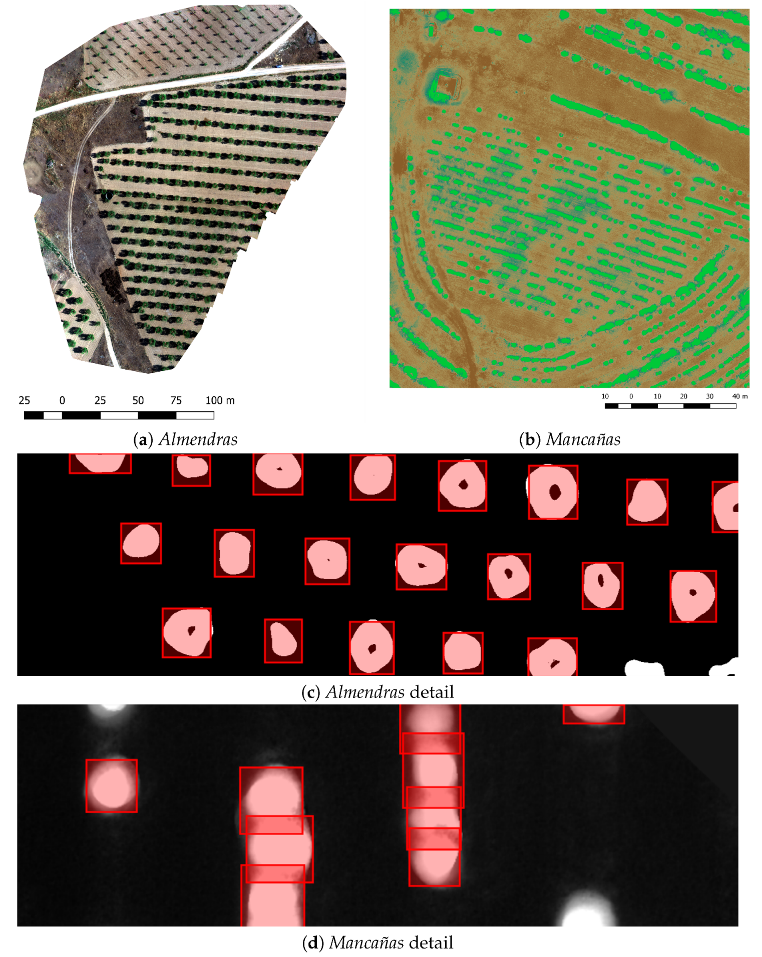
For our experiments, we flew over two different locations (see Figure 5 and Figure 6): Almendras and Mancañas. The Almendras is a 3.5 hectare (ha) leaf-on almond (Prunus dulcis) tree plantation with a mean distance between the trees of m located near Valencia, Spain. The Mancañas, in Guanajuato, Mexico, is a 0.76 ha leaf-on pine (Pinus greggii) with rows of trees and a mean distance between rows of m. However, within the rows, the trees have a mean distance of m.
The hardware employed to run the computer vision and image analysis algorithms consisted of a computer to implement the classical approaches and a second one for the deep learning-based methods (see Section 3.3 and Table 2). The former consists of a Windows 8.1 machine with an i7-3770 CPU at 3.4 GHz, 16 GB of RAM. The latter is a computer running Ubuntu 16.04 xenial with a liquid-cooled Intel Xeon E5-2650 CPU, 32 GB of RAM, four Nvidia Titan X Pascal GPUs, each one with 12 GB of video memory.
4.1. Tree Detection
We trained our treetop detection methods using synthetic images and evaluated the performance on the images produced at the Almendras and Mancañas test fields. To train the deep learning-based approaches for treetop detection, we generated a synthetic-labeled data set of 12,500 synthetic DEVM images of pixels that simulate a resolution of 1 cm/pixel with the values described in Table 1. We split the 12,500 images synthetic data set into two subsets of 10,000 images for training and 2500 images for validation at refinement. We refined the neural network weights during ten epochs. The structure of the neural network models that we tested require three-channel images. Thus, to feed the network, we converted the DEVM to RGB images using OpenCV’s cvtColor function, which replicates the DVEM image in each of the three channels. This process facilitated using the synthetic database on off-the-shelf neural network models requiring three-channel images, of course, at the expense of additional weights in the first convolutional layer.
We tested the efficiency of the different methods in the Almendras and Mancañas DEVM orthomosaic images containing pine (Pinus greggii) and almond (Prunus dulcis) trees, respectively. We evaluated our approach’s performance by comparing the detections with manually obtained ground truth data (see Figure 7 and Figure 8). We considered a detection when the Intersection of the Union (IoU) is at least 0.50 between the predicted and the ground truth bounding boxes.
We processed the individual images from our test fields with Pix4D to generate GeoTIFF orthomosaics with a size of and pixels for the Almendras and Mancañas, respectively. Since these images are too large for the computer’s memory, we divided them into smaller overlapping clips of pixels (resulting in 176 images for the Almendras and 504 images for the Mancañas) which in turn were fed to the different methods for treetop detection. Afterward, we expressed the results on a global reference system and applied non-maximal suppression.
4.2. Results
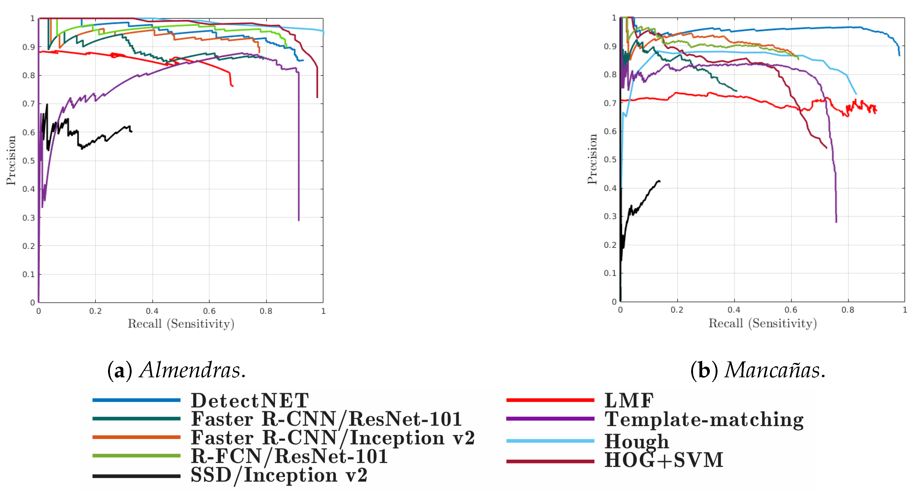
We trained and fine-tuned the algorithms using the synthetic data set, while employed the Mancañas and the Almendras data sets to test without making a change to the parameters to obtain the respective performance metrics. To evaluate the performance of the different algorithms involved in the comparison, we applied the methods to the Almendras and Mancañas tree stands and evaluated different metrics, including Precision, Recall, Average Precision, Average Recall, and . In Figure 8, we show the Precision-Recall curves resulting from varying the acceptation threshold for detection. We obtained each point of the curve by discarding those detections whose confidence score was under the threshold. The companion Table 2 highlights quantitatively some characteristics of the curves in Figure 8. In particular, it provides indicators such as the Average Precision, , Average Recall, , and the metric . The columns , , and follow the Pascal VOC [70] criterion, where an object is correctly detected when the IoU between its prediction and the ground truth bounding boxes is larger or equal to 0.5. Thus, corresponds to the maximum value of the metric for the criterion IoU ≥ 0.5.
For the Template method, we selected the correlation template from the synthetic DEVM database and applied it to both Almendras and Mancañas fields. Note that consistently, the Almendras tree stand gave better results than the Mancañas tree stand for the , , and metrics. Despite low averages for and , the LMF method, with , obtained the second highest value for the Almendras. Its behavior in the Mancañas observed just slight fluctuations with values 0.700, 0.774 and 0.797 for , and , respectively. The Hough method obtained the highest value at 0.950 in the Almendras. Interestingly, in the same metric had an abrupt decrement, at 0.442, in the Mancañas. It is worth noting that both methods are easy to code and exhibit low computing complexity. Template-matching had a regular performance in both the Almendras and the Mancañas, perhaps justifying the common practice of selecting the template from samples of the same image where it is going to operate but underscoring its fragility to diversity. For HOG+SVM, we computed the HOG features using training examples from the synthetic data set and tested on the Almendras and the Mancañas fields, performing better across our metrics in the former (0.794, 0.914, 0.92) than in the latter (0.659, 0.644, 0.663) for , , and , respectively. These results show the ability of the DEVM synthetic database to generalize well.
Applying the deep learning-based methods, SSD/Inception v2 observed the lowest performance for both tree stands. DetectNET performed better for the Almendras in terms of , at 0.880, but was outperformed by R-FCN/ResNet-101 in terms of , at 0.922. In all other cases, the deep learning methods performance was weaker for the Mancañas data set than for the Almendras one. A noticeable exception was the DetectNet method, which actually had a better performance for the Mancañas with , , and . Interestingly, Faster R-CNN, both with the Inception v2 and ResNet-101 backbones, has comparable performance in the Almendras but the Inception v2 backbone performed better in the Mancañas tree stand. R-FCN with ResNet-101 backbone was the best for the metric, at 0.922, for the Almendras but its , and declined sharply for the Mancañas at 0.571, 0.577 and 0.723, respectively. In terms of computing time (see Table 2), LMF was the fastest, and it does not require training. About the methods requiring some form of training, the Template method was the quickest one during this stage. In addition, among the neural network-based approaches, Faster R-CNN/Inception was the faster one to train. HOG+SVM was the fastest one during the evaluation stage, taking about two seconds to process a whole orthomosaic. Among the deep learning-based techniques, SSD/Inception v2 was the fastest one, taking two minutes and two seconds to evaluate the entire image.
5. Discussion
The DEVM representation permitted us to blend structural and multispectral information efficiently. The DEVM facilitated us to generate synthetic images, which can be used effectively to train classical and modern tree detection methods. This observation aligns with Perez et al. [71], who have highlighted the importance of incorporating the NDVI as an input to foster the performance of automatic tree detection algorithms. However, for a precise estimation of vegetation indices, one needs to consider some crucial factors, including illumination geometry and flying height, which may play a significant role in surface reflectance determination [72]. In our work, we used the built-in Pix4D conversion formula to obtain the derived NDVI, but we may need to investigate further whether a more robust radiometric calibration could enhance tree detection performance [73].
Our synthetic data set includes images with a wide range of tree spacing and crown characteristics, including size, height, and shape. Therefore, it seems that neural network-based methods may generalize well for different forest types. In contrast to template matching, such approaches do not require producing a template describing a particular experimental forest [61]. We believe that the deep learning approach provides a unified framework where different tree models interact, making it easier to generalize. One could consider a CNN as a generalization of template matching where training supports the estimation of the most appropriate convolutional masks for detection [74]. This interpretation could explain the similar performance to DetectNET obtained in the Almendras tree stand.
Simple methods, such as LMF and Hough, performed consistently well. They can be programmed easily using widely available computer vision libraries and require humble computing platforms. From our perspective, this result confirms the often neglected value of classic approaches [75]. Perhaps, the most surprising result was the differential performance exhibited by the deep learning methods in the Mancañas test field. Certainly, detecting individual trees in the Mancañas is more difficult than in the Almendras site (see Figure 5c,d). In the latter, the trees are isolated, while in the former, the rows are isolated, but the trees within are clustered. Our results show the value of DetectNet as an object detection model based on coverage maps rather than the anchor-based models such as Faster R-CNN, SSD, and R-FCN [76]. Although they share the same backbone architecture in some cases, the bounding box extraction strategy may show different performance for specific scenarios [77]. However, further studies are needed to understand the effects of deep learning architectures in the generation of covering maps [78]. In our experiments, the DetectNet representation exhibited better performance than the region-based proposal architectures.
6. Conclusions
In this paper, we describe methods to assess treetop detection methodologies efficiently. The DEVM representation made it possible to develop a strategy to construct synthetic ground truth data useful for training, alleviating the need for the task of labeling images. The representation compares well when benchmarked with classic and deep learning-based algorithms. Our experiments with data sets from two different forests provide support for our claims.
Although our results suggest that the methods can accommodate a limited degree of tree overlaps, further research is required to extend them to more challenging scenarios, such as the conditions of overlapping crowns often found in dense forests. Nonetheless, our experiments were successful in two different settings, including broadleaf and evergreen (needle leaf) trees, suggesting that we can apply the methods to other scenarios.
We plan to formulate the input to the CNN models with the raw data constituted by the near-infrared and red images, and the DMT and DSM maps. We expect that the neural network will unveil an optimized combination of the inputs to improve performance. We will also incorporate tree detection methods to a pipeline where SfM reconstruction and tree identification could be combined with allometric equations to obtain estimates of the stored carbon dioxide. Finally, we will continue developing algorithms for the detection of trees in more complex scenarios, such as urban areas or forests.
Author Contributions
Conceptualization, M.R. and J.S.; methodology, J.S.; software, D.P. and J.S.; validation, D.P., K.P. and J.S.; formal analysis, D.P., M.R., and J.S.; investigation, D.P. and J.S.; resources, S.K. and J.S.; data curation, D.P.; writing–initial draft preparation, D.P., J.S.; writing–review and editing, D.P., J.S., M.R., K.P., S.K.; visualization, D.P. and J.S.; supervision, J.S., M.R., and S.K.; project administration, J.S.; funding acquisition, S.K. and J.S. All authors have read and agreed to the published version of the manuscript.
Funding
This work was partially funded by SIP-IPN 20201357 for Joaquín Salas.
Acknowledgments
We thank Bert Rijk, from Aurea Imaging, for providing us the images from Valencia. Also, we thank Othón González for piloting the UAS from where we extracted some of the images and to Heladio Rubio for granting us access to his tree plot. Thanks to RAPTOR for its Phantom-3.
Conflicts of Interest
The authors declare no conflict of interest. The funders had no role in the design of the study; in the collection, analyses, or interpretation of data; in the writing of the manuscript, or in the decision to publish the results.
Appendix A. Pipeline for the Creation of Synthetic Images
The following algorithm describes our procedure to create synthetic DEVM images for training.
| Algorithm A1 Synthetic DEVM images of trees. We generated domes to define individual tree shapes. The pdf generated random real values from a uniform distribution in the range between a and b, inclusive. is the floor function. | |
| 1: Call: | |
| 2: Input: The number of rows r and columns c for the output image | |
| 3: Output: Synthetic DEVM image, | |
| ▹ Assume the existence of global constants , , and , the minimum and maximum number of trees, number domes per tree, and height of the trees, respectively; and , the minimum and maximum lateral widths of each dome, correspondingly; , the maximum displacement of the centroid and the change of the width, respectively; and and , a diagonal matrix with the relationship between meters and pixels, and the center of the dome in the image. | |
| 4: ; | ▹ Initialize DEVM image to zero |
| 5: ; | ▹ Define the number of trees |
| 6: for do | |
| 7: ; | ▹i-th tree height |
| 8: ; | |
| 9: ; | ▹i-th tree width |
| 10: ; | |
| 11: ; | |
| ▹i-th tree center | |
| 12: ; | ▹ number of domes for the i-th tree |
| 13: for do | |
| 14: ; | ▹ height for the j-th domes of the i-th tree |
| 15: ; | |
| 16: ; | |
| ▹ center of the j-th dome of the i-th tree | |
| 17: ; | |
| 18: ; | |
| ▹ width of the j-th dome of the i-th tree | |
| 19: | ▹ create a dome using (3) |
| 20: | ▹ transform domains, |
| 21: ; | ▹ Add dome to image |
| 22: end for | |
| 23: end for | |
References
- Kelly, A. Improving REDD+ (Reducing Emissions from Deforestation and Forest Degradation) Programs. Ph.D. Thesis, University of Washington, Washington, DC, USA, 2017. [Google Scholar]
- Lund, G.; Thomas, C. A Primer on Stand and Forest Inventory Designs; Technical Report WO-54; US Department of Agriculture Forest Service: Los Angeles, CA, USA, 1989. [Google Scholar]
- Özyeşil, O.; Voroninski, V.; Basri, R.; Singer, A. A Survey of Structure from Motion. Acta Numer. 2017, 26, 305–364. [Google Scholar] [CrossRef]
- Zhang, Y.; Zhang, Y.; Yunjun, Z.; Zhao, Z. A Two-Step Semiglobal Filtering Approach to Extract DTM From Middle Resolution DSM. IEEE Geosci. Remote Sens. Lett. 2017, 14, 1599–1603. [Google Scholar] [CrossRef]
- Carlson, T.; Ripley, D. On the Relation between NDVI, Fractional Vegetation Cover, and Leaf Area Index. Remote Sens. Environ. 1997, 62, 241–252. [Google Scholar] [CrossRef]
- Ozdarici-Ok, A. Automatic Detection and Delineation of Citrus Trees from VHR Satellite Imagery. Int. J. Remote Sens. 2015, 36, 4275–4296. [Google Scholar] [CrossRef]
- Gomes, M.; Maillard, P. Detection of Tree Crowns in Very High Spatial Resolution Images. Environ. Appl. Remote. Sens. 2016. [Google Scholar] [CrossRef] [Green Version]
- Koc-San, D.; Selim, S.; Aslan, N.; San, B. Automatic Citrus Tree Extraction from UAV Images and Digital Surface Models using Circular Hough Transform. Comput. Electron. Agric. 2018, 150, 289–301. [Google Scholar] [CrossRef]
- Özcan, A.; Hisar, D.; Sayar, Y.; Ünsalan, C. Tree Crown Detection and Delineation in Satellite Images using Probabilistic Voting. Remote Sens. Lett. 2017, 8, 761–770. [Google Scholar] [CrossRef]
- Shafarenko, L.; Petrou, M.; Kittler, J. Automatic Watershed Segmentation of Randomly Textured Color Images. IEEE Trans. Image Process. 1997, 6, 1530–1544. [Google Scholar] [CrossRef]
- Reza, N.; Na, S.; Lee, K. Automatic Counting of Rice Plant Numbers after Transplanting using Low Altitude UAV Images. Int. J. Contents 2017, 13, 1–8. [Google Scholar]
- Maillard, P.; Gomes, M. Detection and Counting of Orchard Trees from VHR Images using a Geometrical-Optical Model and Marked Template Matching. ISPRS Ann. Photogramm. Remote Sens. Spat. Inf. Sci. 2016, 3, 75. [Google Scholar] [CrossRef]
- Bao, Y.; Tian, Q.; Chen, M.; Lin, H. An Automatic Extraction Method for Individual Tree Crowns based on Self-Adaptive Mutual Information and Tile Computing. Int. J. Digit. Earth 2015, 8, 495–516. [Google Scholar] [CrossRef]
- Goldbergs, G.; Maier, S.; Levick, S.; Edwards, A. Efficiency of Individual Tree Detection Approaches Based on Light-Weight and Low-Cost UAS Imagery in Australian Savannas. Remote Sens. 2018, 10, 161. [Google Scholar] [CrossRef] [Green Version]
- Fassnacht, F.; Mangold, D.; Schäfer, J.; Immitzer, M.; Kattenborn, T.; Koch, B.; Latifi, H. Estimating Stand Density, Biomass and Tree Species from Very High Resolution Stereo-Imagery–Towards an All-in-One Sensor for Forestry Applications. For. Int. J. For. Res. 2017, 90, 1–19. [Google Scholar] [CrossRef]
- Wang, Y.; Zhu, X.; Wu, B. Automatic Detection of Individual Oil Palm Trees from UAV Images using HOG Features and an SVM Classifier. Int. J. Remote Sens. 2018, 40, 1–15. [Google Scholar] [CrossRef]
- Li, W.; He, C.; Fu, H.; Zheng, J.; Dong, R.; Yu, L.; Luk, W. A Real-Time Tree Crown Detection Approach for Large-Scale Remote Sensing Images on FPGAs. Remote Sens. 2019, 11, 1025. [Google Scholar] [CrossRef] [Green Version]
- Xiao, C.; Qin, R.; Xie, X.; Huang, X. Individual Tree Detection and Crown Delineation with 3D Information from Multi-view Satellite Images. Photogramm. Eng. Remote Sens. 2019, 85, 55–63. [Google Scholar] [CrossRef] [Green Version]
- García, D.; Caicedo, J.; Castellanos, G. Individual Detection of Citrus and Avocado Trees Using Extended Maxima Transform Summation on Digital Surface Models. Remote Sens. 2020, 12, 1633. [Google Scholar] [CrossRef]
- Tianyang, D.; Jian, Z.; Sibin, G.; Ying, S.; Jing, F. Single-Tree Detection in High-Resolution Remote-Sensing Images Based on a Cascade Neural Network. ISPRS Int. J. Geo Inf. 2018, 7, 367. [Google Scholar] [CrossRef] [Green Version]
- Guo, Y.; Liu, Y.; Oerlemans, A.; Lao, S.; Wu, S.; Lew, M. Deep Learning for Visual Understanding: A Review. Neurocomputing 2016, 187, 27–48. [Google Scholar] [CrossRef]
- Freudenberg, M.; Nölke, N.; Agostini, A.; Urban, K.; Wörgötter, F.; Kleinn, C. Large Scale Palm Tree Detection In High Resolution Satellite Images Using U-Net. Remote Sens. 2019, 11, 312. [Google Scholar] [CrossRef] [Green Version]
- Li, W.; Dong, R.; Fu, H.; Yu, L. Large-Scale Oil Palm Tree Detection from High-Resolution Satellite Images Using Two-Stage Convolutional Neural Networks. Remote Sens. 2019, 11, 11. [Google Scholar] [CrossRef] [Green Version]
- Zortea, M.; Nery, M.; Ruga, B.; Carvalho, L.; Bastos, A. Oil-Palm Tree Detection in Aerial Images Combining Deep Learning Classifiers. In Proceedings of the IEEE International Geoscience and Remote Sensing Symposium, Valencia, Spain, 22–27 July 2018; pp. 657–660. [Google Scholar]
- Csillik, O.; Cherbini, J.; Johnson, R.; Lyons, A.; Kelly, M. Identification of Citrus Trees from Unmanned Aerial Vehicle Imagery using Convolutional Neural Networks. Drones 2018, 2, 39. [Google Scholar] [CrossRef] [Green Version]
- Li, W.; Fu, H.; Yu, L.; Cracknell, A. Deep Learning based Oil Palm Tree Detection and Counting for High-Resolution Remote Sensing Images. Remote Sens. 2016, 9, 22. [Google Scholar] [CrossRef] [Green Version]
- Li, W.; Fu, H.; Yu, L. Deep Convolutional Neural Network based Large-Scale Oil Palm Tree Detection for High-Resolution Remote Sensing Images. In Proceedings of the IEEE International Geoscience and Remote Sensing Symposium, Fort Worth, TX, USA, 23–28 July 2017; pp. 846–849. [Google Scholar]
- Mubin, N.; Nadarajoo, E.; Shafri, H.; Hamedianfar, A. Young and Mature Oil Palm Tree Detection and Counting using Convolutional Neural Network Deep Learning Method. Int. J. Remote Sens. 2019, 40, 7500–7515. [Google Scholar] [CrossRef]
- Cheang, E.; Cheang, T.; Tay, Y. Using Convolutional Neural Networks to Count Palm Trees in Satellite Images. arXiv 2017, arXiv:1701.06462. [Google Scholar]
- Fan, Z.; Lu, J.; Gong, M.; Xie, H.; Goodman, E.D. Automatic Tobacco Plant Detection in UAV Images via Deep Neural Networks. IEEE J. Sel. Top. Appl. Earth Obs. Remote Sens. 2018, 11, 876–887. [Google Scholar] [CrossRef]
- Trier, Ø.; Salberg, A.B.; Kermit, M.; Rudjord, Ø.; Gobakken, T.; Næsset, E.; Aarsten, D. Tree Species Classification in Norway from Airborne Hyperspectral and Airborne Laser Scanning Data. Eur. J. Remote Sens. 2018, 51, 336–351. [Google Scholar] [CrossRef]
- Windrim, L.; Bryson, M. Forest Tree Detection and Segmentation using High Resolution Airborne LiDAR. arXiv 2018, arXiv:1810.12536. [Google Scholar]
- Pibre, L.; Chaumont, M.; Subsol, G.; Ienco, D.; Derras, M. How to Deal with Multi-Source Data for Tree Detection based on Deep Learning. In Proceedings of the 2017 IEEE Global Conference on Signal and Information Processing (GlobalSIP), Montreal, QC, Canada, 14–16 November 2017. [Google Scholar]
- Chen, S.; Shivakumar, S.; Dcunha, S.; Das, J.; Okon, E.; Qu, C.; Taylor, C.; Kumar, V. Counting Apples and Oranges with Deep Learning: A Data-Driven Approach. IEEE Robot. Autom. Lett. 2017, 2, 781–788. [Google Scholar] [CrossRef]
- Zakharova, M. Automated Coconut Tree Detection in Aerial Imagery Using Deep Learning. Ph.D. Thesis, The Katholieke Universiteit Leuven, Löwen, Belgium, 2017. [Google Scholar]
- Puttemans, S.; Van Beeck, K.; Goedemé, T. Comparing Boosted Cascades to Deep Learning Architectures for Fast and Robust Coconut Tree Detection in Aerial Images. In Proceedings of the 13th International Joint Conference on Computer Vision, Imaging and Computer Graphics Theory and Applications, Madeira, Portugal, 27–29 January 2018. [Google Scholar]
- Zortea, M.; Macedo, M.; Britto, A.; Ruga, B. Automatic Citrus Tree Detection from UAV Images based on Convolutional Neural Networks. In Proceedings of the 2018 31th SIBGRAPI Conference on Graphics, Patterns and Images (SIBGRAPI), Foz Do Iguaçu, Brazil, 29 October–1 November 2018. [Google Scholar]
- Viola, P.; Jones, M. Rapid Object Detection using a Boosted Cascade of Simple Features. In Proceedings of the IEEE Conference on Computer Vision and Pattern Recognition, Kauai, HI, USA, 8–14 December 2001; Volume 1, pp. I-511–I-518. [Google Scholar]
- Dollár, P.; Appel, R.; Belongie, S.; Perona, P. Fast Feature Pyramids for Object Detection. IEEE Trans. Pattern Anal. Mach. Intell. 2014, 36, 1532–1545. [Google Scholar] [CrossRef] [Green Version]
- Ribera, J.; Chen, Y.; Boomsma, C.; Delp, E. Plant Leaf Segmentation for Estimating Phenotypic Traits. In Proceedings of the IEEE International Conference on Image Processing, Beijing, China, 17–20 September 2017. [Google Scholar]
- Xiao, C.; Qin, R.; Huang, X.; Li, J. A Study of using Fully Convolutional Network for Treetop Detection on Remote Sensing Data. ISPRS Ann. Photogramm. Remote Sens. Spat. Inf. Sci. 2018, 4. [Google Scholar] [CrossRef] [Green Version]
- Long, J.; Shelhamer, E.; Darrell, T. Fully Convolutional Networks for Semantic Segmentation. In Proceedings of the IEEE Conference on Computer Vision and Pattern Recognition, Boston, MA, USA, 7–12 June 2015; pp. 3431–3440. [Google Scholar]
- Santos, A.D.; Marcato, J.; Araújo, M.S.; Di Martini, D.; Tetila, E.; Siqueira, H.; Aoki, C.; Eltner, A.; Matsubara, E.; Pistori, H.; et al. Assessment of CNN-Based Methods for Individual Tree Detection on Images Captured by RGB Cameras Attached to UAVs. Sensors 2019, 19, 3595. [Google Scholar] [CrossRef] [PubMed] [Green Version]
- Fromm, M.; Schubert, M.; Castilla, G.; Linke, J.; McDermid, G. Automated Detection of Conifer Seedlings in Drone Imagery Using Convolutional Neural Networks. Remote Sens. 2019, 11, 2585. [Google Scholar] [CrossRef] [Green Version]
- Ubbens, J.; Cieslak, M.; Prusinkiewicz, P.; Stavness, I. The Use of Plant Models in Deep Learning: An Application to Leaf Counting in Rosette Plants. Plant Methods 2018, 14, 6. [Google Scholar] [CrossRef] [Green Version]
- Han, S.; Kerekes, J. Overview of Passive Optical Multispectral and Hyperspectral Image Simulation Techniques. IEEE J. Sel. Top. Appl. Earth Obs. Remote Sens. 2017, 10, 4794–4804. [Google Scholar] [CrossRef]
- Fassnacht, F.; Latifi, H.; Hartig, F. Using Synthetic Data to Evaluate the Benefits of Large Field Plots for Forest Biomass Estimation with LiDAR. Remote Sens. Environ. 2018, 213, 115–128. [Google Scholar] [CrossRef]
- Pretzsch, H.; Biber, P.; Ďurskỳ, J. The Single Tree-based Stand Simulator SILVA: Construction, Application and Evaluation. For. Ecol. Manag. 2002, 162, 3–21. [Google Scholar] [CrossRef]
- Selim, S.; Sonmez, N.K.; Coslu, M.; Onur, I. Semi-automatic Tree Detection from Images of Unmanned Aerial Vehicle Using Object-Based Image Analysis Method. J. Indian Soc. Remote. Sens. 2019, 47, 193–200. [Google Scholar] [CrossRef]
- Krisanski, S.; Taskhiri, M.S.; Turner, P. Enhancing Methods for Under-Canopy Unmanned Aircraft System based Photogrammetry in Complex Forests for Tree Diameter Measurement. Remote Sens. 2020, 12, 1652. [Google Scholar] [CrossRef]
- Qiu, L.; Jing, L.; Hu, B.; Li, H.; Tang, Y. A New Individual Tree Crown Delineation Method for High Resolution Multispectral Imagery. Remote Sens. 2020, 12, 585. [Google Scholar] [CrossRef] [Green Version]
- Picos, J.; Bastos, G.; Míguez, D.; Alonso, L.; Armesto, J. Individual Tree Detection in a Eucalyptus Plantation Using Unmanned Aerial Vehicle (UAV)-LiDAR. Remote Sens. 2020, 12, 885. [Google Scholar] [CrossRef] [Green Version]
- Yan, W.; Guan, H.; Cao, L.; Yu, Y.; Li, C.; Lu, J. A Self-Adaptive Mean Shift Tree-Segmentation Method using UAV LiDAR Data. Remote Sens. 2020, 12, 515. [Google Scholar] [CrossRef] [Green Version]
- Weinstein, B.G.; Marconi, S.; Bohlman, S.; Zare, A.; White, E. Individual tree-crown detection in RGB imagery using semi-supervised deep learning neural networks. Remote Sens. 2019, 11, 1309. [Google Scholar] [CrossRef] [Green Version]
- Rouse, J.; Haas, R.; Schell, J.; Deering, D. Monitoring Vegetation Systems in the Great Plains with ERTS. In Proceedings of the Third Earth Resources Technology Satellite—1 Symposium; NASA: Washington, DC, USA, 1974. [Google Scholar]
- Weier, J.; Herring, D. Measuring Vegetation (NDVI & EVI); NASA Earth Observatory: Greenbelt, MD, USA, 2000. [Google Scholar]
- Gu, Y.; Wylie, B.K.; Howard, D.; Phuyal, K.; Ji, L. NDVI Saturation Adjustment: A New Approach for Improving Cropland Performance Estimates in the Greater Platte River Basin, USA. Ecol. Indic. 2013, 30, 1–6. [Google Scholar] [CrossRef]
- Liu, F.; Qin, Q.; Zhan, Z. A Novel Dynamic Stretching Solution to Eliminate Saturation Effect in NDVI and its Application in Drought Monitoring. Chin. Geogr. Sci. 2012, 22, 683–694. [Google Scholar] [CrossRef]
- Lin, T.Y.; Maire, M.; Belongie, S.; Hays, J.; Perona, P.; Ramanan, D.; Dollár, P.; Zitnick, L. Microsoft COCO: Common Objects in Context. In European Conference on Computer Vision; Springer: Berlin/Heidelberg, Germany, 2014; pp. 740–755. [Google Scholar]
- Pouliot, D.; King, D.; Bell, F.; Pitt, D. Automated Tree Crown Detection and Delineation in High-Resolution Digital Camera Imagery of Coniferous Forest Regeneration. Remote Sens. Environ. 2002, 82, 322–334. [Google Scholar] [CrossRef]
- Ke, Y.; Quackenbush, L. A Review of Methods for Automatic Individual Tree-Crown Detection and Delineation from Passive Remote Sensing. Int. J. Remote Sens. 2011, 32, 4725–4747. [Google Scholar] [CrossRef]
- Dalal, N.; Triggs, B. Histograms of Oriented Gradients for Human Detection. In Proceedings of the IEEE International Conference on Computer Vision and Pattern Recognition, San Diego, CA, USA, 20–25 June 2005; Volume 1, pp. 886–893. [Google Scholar]
- Barker, J.; Sarathy, S.; Tao, A. DetectNet: Deep Neural Network for Object Detection in DIGITS. 2016. Available online: https://tinyurl.com/detectnet (accessed on 30 November 2016).
- Redmon, J.; Divvala, S.; Girshick, R.; Farhadi, A. You Only Look Once: Unified, Real-Time Object Detection. In Proceedings of the IEEE Conference on Computer Vision and Pattern Recognition, Las Vegas, NV, USA, 27–30 June 2016; pp. 779–788. [Google Scholar]
- Szegedy, C.; Liu, W.; Jia, Y.; Sermanet, P.; Reed, S.; Anguelov, D.; Erhan, D.; Vanhoucke, V.; Rabinovich, A. Going Deeper with Convolutions. In Proceedings of the IEEE Conference on Computer Vision and Pattern Recognition, Boston, MA, USA, 7–12 June 2015; pp. 1–9. [Google Scholar]
- Geiger, A.; Lenz, P.; Stiller, C.; Urtasun, R. Vision meets Robotics: The KITTI Dataset. Int. J. Robot. Res. 2013, 32, 1231–1237. [Google Scholar] [CrossRef] [Green Version]
- Ren, S.; He, K.; Girshick, R.; Sun, J. Faster R-CNN: Towards Real-Time Object Detection with Region Proposal Networks. In Proceedings of the Advances in Neural Information Processing Systems, Montreal, QC, Canada, 7–12 November 2015; pp. 91–99. [Google Scholar]
- Liu, W.; Anguelov, D.; Erhan, D.; Szegedy, C.; Reed, S.; Fu, C.Y.; Berg, A. SSD: Single-Shot Multibox Detector. In European Conference on Computer Vision; Springer: Berlin/Heidelberg, Germany, 2016; pp. 21–37. [Google Scholar]
- Tieleman, T.; Hinton, G. Lecture 6.5—RmsProp: Divide the Gradient by a Running Average of its Recent Magnitude. Coursera Neural Networks Mach. Learn. 2012, 4, 26–31. [Google Scholar]
- Everingham, M.; Van Gool, L.; Williams, C.; Winn, J.; Zisserman, A. The Pascal Visual Object Classes (VOC) Challenge. Int. J. Comput. Vis. 2010, 88, 303–338. [Google Scholar] [CrossRef] [Green Version]
- Pérez-Bueno, M.; Pineda, M.; Vida, C.; Fernández-Ortuño, D.; Torés, J.; de Vicente, A.; Cazorla, F.; Barón, M. Detection of White Root Rot in Avocado Trees by Remote Sensing. Plant Dis. 2019, 103, 1119–1125. [Google Scholar] [CrossRef] [PubMed]
- Stow, D.; Nichol, C.; Wade, T.; Assmann, J.; Simpson, G.; Helfter, C. Illumination Geometry and Glying Height Influence Surface Reflectance and NDVI Derived from Multispectral UAS Imagery. Drones 2019, 3, 55. [Google Scholar] [CrossRef] [Green Version]
- Fawcett, D.; Panigada, C.; Tagliabue, G.; Boschetti, M.; Celesti, M.; Evdokimov, A.; Biriukova, K.; Colombo, R.; Miglietta, F.; Rascher, U.; et al. Multi-Scale Evaluation of Drone-Based Multispectral Surface Reflectance and Vegetation Indices in Operational Conditions. Remote Sens. 2020, 12, 514. [Google Scholar] [CrossRef] [Green Version]
- Goodfellow, I.; Bengio, Y.; Courville, A.; Bengio, Y. Deep Learning; MIT Press: Cambridge, UK, 2016; Volume 1. [Google Scholar]
- Marcus, G. Deep Learning: A Critical Appraisal. arXiv 2018, arXiv:1801.00631. [Google Scholar]
- Huang, J.; Rathod, V.; Sun, C.; Zhu, M.; Korattikara, A.; Fathi, A.; Fischer, I.; Wojna, Z.; Song, Y.; Guadarrama, S. Speed/Accuracy Trade-offs for Modern Convolutional Object Detectors. In Proceedings of the IEEE Computer Vision and Pattern Recognition, Honolulu, HI, USA, 21–26 July 2017; pp. 7310–7311. [Google Scholar]
- Wang, H.; Yu, Y.; Cai, Y.; Chen, X.; Chen, L.; Liu, Q. A Comparative Study of State-of-the-Art Deep Learning Algorithms for Vehicle Detection. IEEE Intell. Transp. Syst. Mag. 2019, 11, 82–95. [Google Scholar] [CrossRef]
- Lenc, K. Representation of Spatial Transformations in Deep Neural Networks. Ph.D. Thesis, University of Oxford, Oxford, UK, 2018. [Google Scholar]
Figure 1.
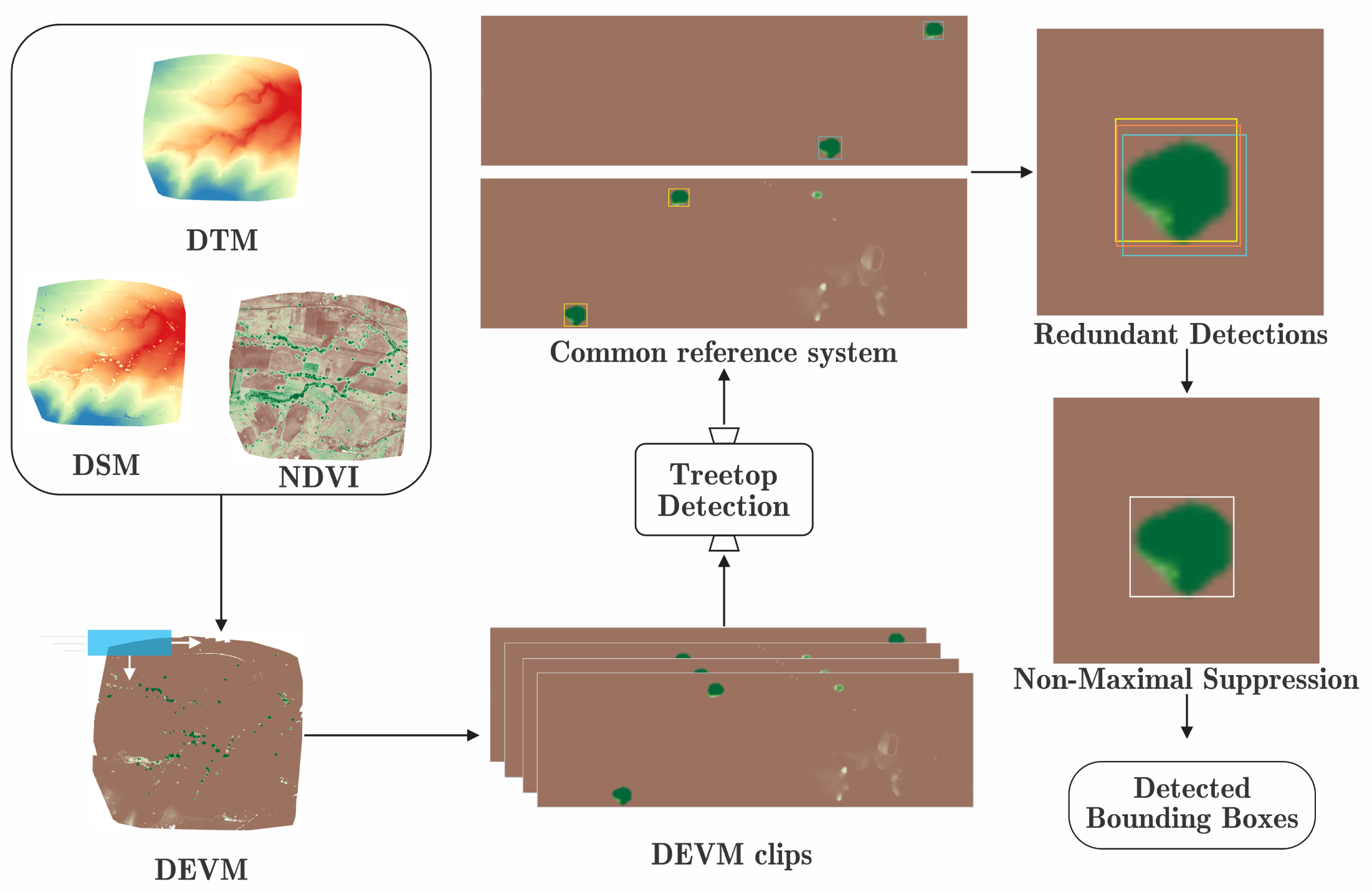
A pipeline to automatically detect treetops. Aerial photogrammetry, obtained from unoccupied aerial systems (UAS) using multispectral cameras, allows us to construct orthomosaics representing the digital surface model (DSM), digital terrain model (DTM), and Normalized Difference Vegetation Index (NDVI), from which we eventually build the Digital Elevated Vegetation Model (DEVM). We split the DEVM into sub-images and evaluate them with an object detector, which predicts the bounding boxes for each sub-image. Then, we express the results in a common reference system. Once we obtain a prediction for the whole image, we apply non-maximal suppression to eliminate redundant detections.
Figure 1.
A pipeline to automatically detect treetops. Aerial photogrammetry, obtained from unoccupied aerial systems (UAS) using multispectral cameras, allows us to construct orthomosaics representing the digital surface model (DSM), digital terrain model (DTM), and Normalized Difference Vegetation Index (NDVI), from which we eventually build the Digital Elevated Vegetation Model (DEVM). We split the DEVM into sub-images and evaluate them with an object detector, which predicts the bounding boxes for each sub-image. Then, we express the results in a common reference system. Once we obtain a prediction for the whole image, we apply non-maximal suppression to eliminate redundant detections.

Figure 2.
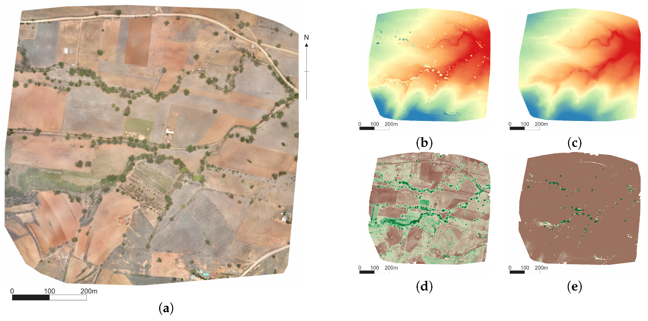
We generated orthomosaic models from multispectral images corresponding to (a) RGB, (b) DSM, (c) DTM, (d) NDVI, and (e) DEVM. The patch of 867 m × 801 m terrain corresponded to an agricultural landscape with scattered trees in Zimatlan, Oaxaca, Mexico.
Figure 2.
We generated orthomosaic models from multispectral images corresponding to (a) RGB, (b) DSM, (c) DTM, (d) NDVI, and (e) DEVM. The patch of 867 m × 801 m terrain corresponded to an agricultural landscape with scattered trees in Zimatlan, Oaxaca, Mexico.

Figure 3.
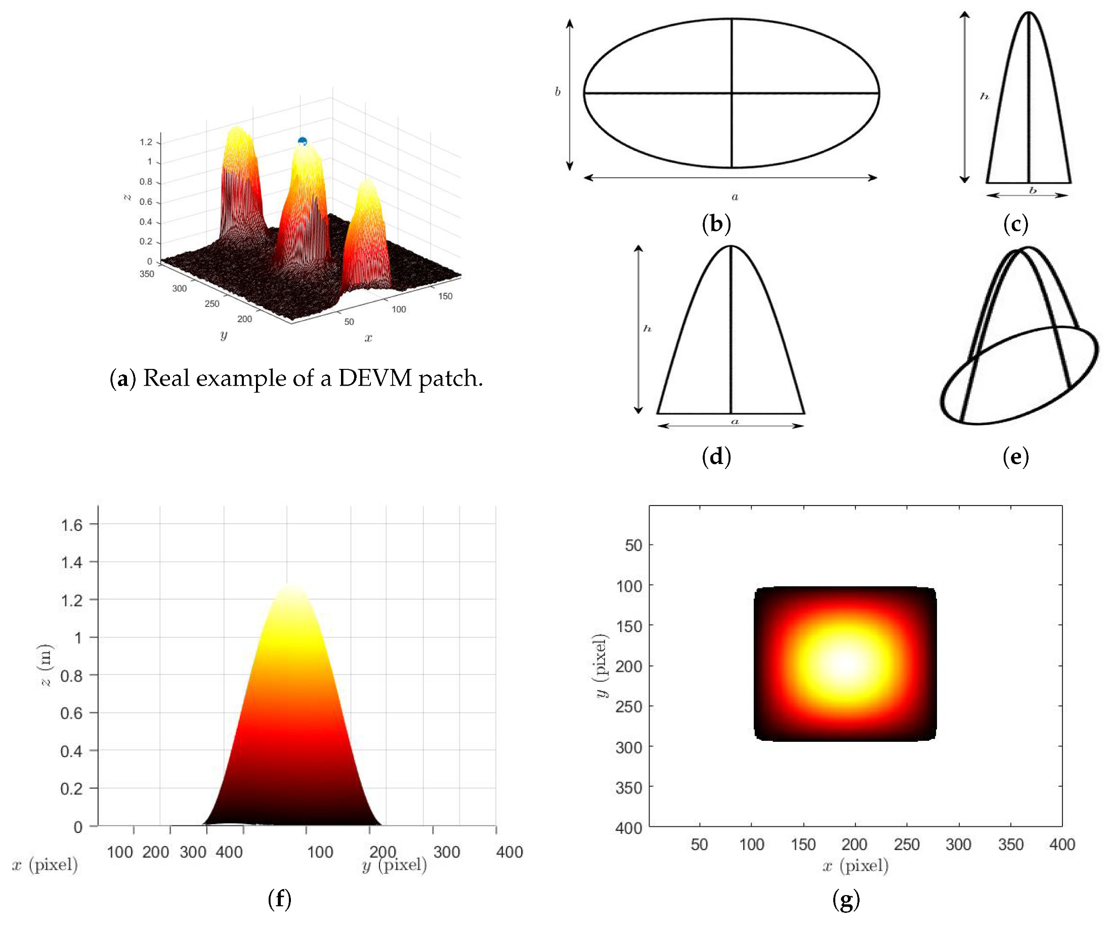
Example of a training data set using DEVM to highlight trees. We built a synthetic data set of trees in the DEVM representation using random ellipses. In (a), we show an example of a DEVM image. We illustrate the orthogonal (b)–(d) and isometric (e) views of a single dome, which forms the basis for the construction of the synthetic representation of a tree in DEVM space. We show an example of the side (f) and top (g) views of the synthetic description.
Figure 3.
Example of a training data set using DEVM to highlight trees. We built a synthetic data set of trees in the DEVM representation using random ellipses. In (a), we show an example of a DEVM image. We illustrate the orthogonal (b)–(d) and isometric (e) views of a single dome, which forms the basis for the construction of the synthetic representation of a tree in DEVM space. We show an example of the side (f) and top (g) views of the synthetic description.

Figure 4.
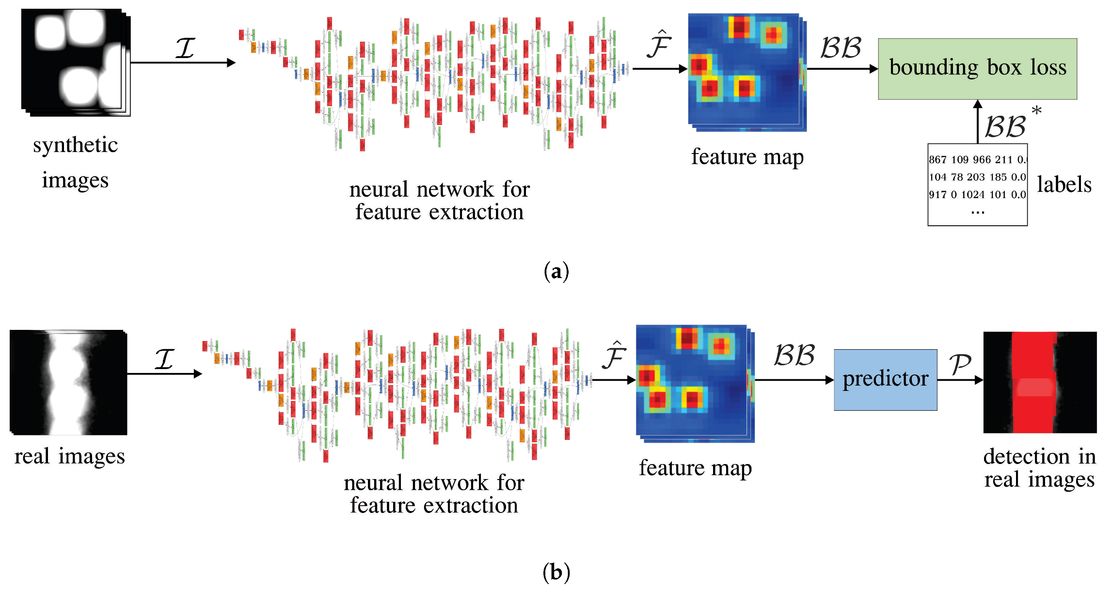
Training and inference of neural network models for treetop detection. We fed a Convolutional Neural Network (CNN) with synthetic DEVM images . During training (a), we utilized synthetic DEVM images to fine-tune the pre-trained weights of the fully connected layers. Then we compared the estimated bounding boxes with the respective ground truth to compute the loss. During evaluation (b), the CNN infers the bounding boxes for real DEVM images to generate predictions .
Figure 4.
Training and inference of neural network models for treetop detection. We fed a Convolutional Neural Network (CNN) with synthetic DEVM images . During training (a), we utilized synthetic DEVM images to fine-tune the pre-trained weights of the fully connected layers. Then we compared the estimated bounding boxes with the respective ground truth to compute the loss. During evaluation (b), the CNN infers the bounding boxes for real DEVM images to generate predictions .

Figure 5.
Test fields. In (a,b), we present the orthomosaics for the whole area of the two places we used to test our method. The Almendras (a) corresponds to almond (Prunus dulcis) trees in Spain, and the Mancañas (b) corresponds to pine (Pinus greggii) trees in Mexico. The DEVM shows that while the trees in the Almendras are isolated (c), in the Mancañas (d) the rows of trees are isolated between them but clustered together within. The bounding boxes in (c,d) show the detections with our method. Please note that viewed from above, almond trees seem to have a hole in the middle.

Figure 6.
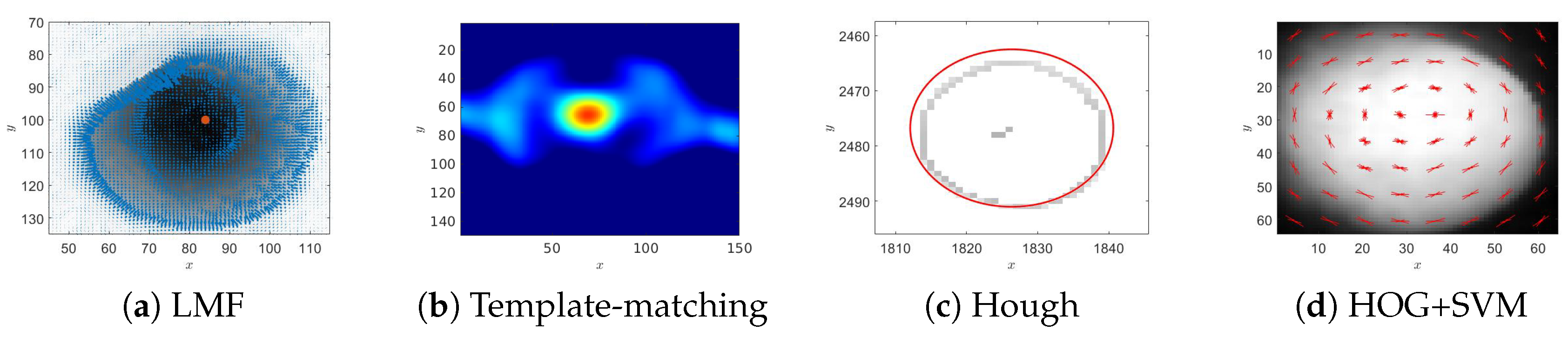
Tree detection with classic methods. In (a), the gradient points toward the maximum, where we place a red dot. In (b), we show the correlation between trees and a template made with synthetic images in the Almendras field. In (c), we show the edges (gray) and a circle fitting the edge points. In (d), we show the HOG descriptors superimposed on the corresponding DEVM patch.
Figure 6.
Tree detection with classic methods. In (a), the gradient points toward the maximum, where we place a red dot. In (b), we show the correlation between trees and a template made with synthetic images in the Almendras field. In (c), we show the edges (gray) and a circle fitting the edge points. In (d), we show the HOG descriptors superimposed on the corresponding DEVM patch.

Figure 7.
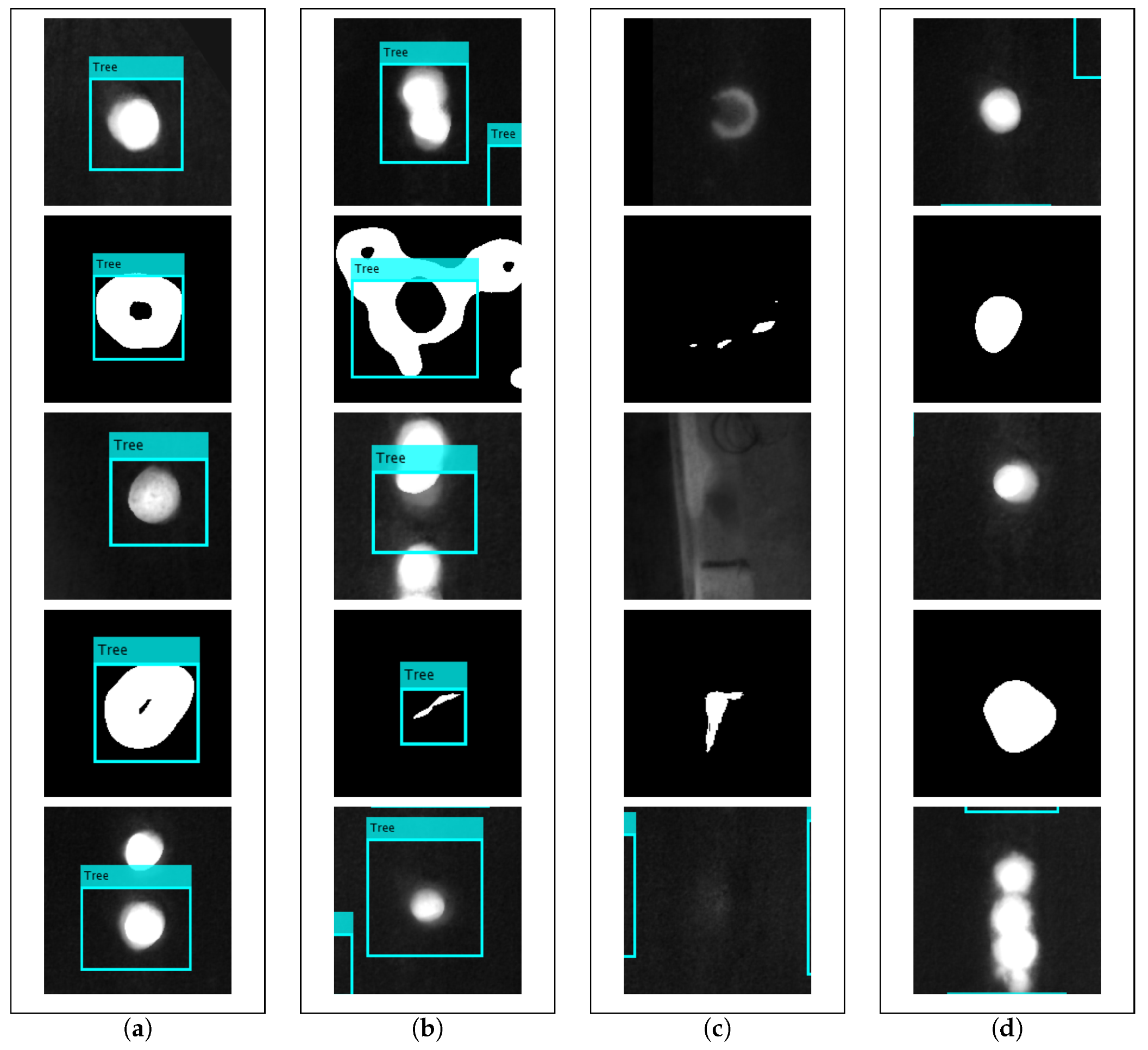
Tree detection. We show the trees in DEVM images with the detected bounding boxes on it. The columns show examples of (a) true positive, (b) false-positive, (c) true-negative, and (d) false negative detection.
Figure 7.
Tree detection. We show the trees in DEVM images with the detected bounding boxes on it. The columns show examples of (a) true positive, (b) false-positive, (c) true-negative, and (d) false negative detection.

Figure 8.
Precision-Recall curves for the methods described in Section 3.3 for the Almendras (a) and the Mancañas (b) tree stands (best seen in color). The curves describe the precision of the methods at different recall levels, varying the confidence score to discard those detections under the threshold. See Table 2 for some quantitative highlights describing the performance.


Table 1.
Constant values used for the generation of synthetic images in Algorithm A1, described in Appendix A.
Table 1.
Constant values used for the generation of synthetic images in Algorithm A1, described in Appendix A.
| r | c | ||||||||||||
|---|---|---|---|---|---|---|---|---|---|---|---|---|---|
| 1248 | 384 | 2 | 7 | 5 | 10 | 1.4 | 2.3 | 65 | 75 | 65 | 75 | 5 | 20 |
Table 2.
Performance results. We tested in the Almendras and Mancañas tree plantations. AP, AR, and stand for the Average Precision, Average Recall, and maximum measures. Bold numbers correspond to the maximum per column. The methods in this table include Local Maximum Filtering (LMF), Template-matching correlation, Hough Transform to detect circles (Hough), and Histograms of Oriented Gradients (HOG) as features followed by a Support Vector Machine (SVM) Classifier (HOG+SVM), DetectNet, Faster Region-based Convolutional Neural Network with Inception v2 as the backbone (Faster R-CNN/Inception v2), Faster Region-based Convolutional Neural Network with ResNet-101 as the backbone (Faster R-CNN/ResNet-101), Single-Shot Multibox Detector with Inception v2 as the backbone (SSD/Inception v2), and Region-based Fully Convolutional Networks with ResNet-101 as the backbone (R-FCN/ResNet-101). The columns show the Average Precision for an IoU of 0.5, , Average Recall for an IoU of 0.5, , and the maximum value for the metric, . Computing Time columns show the time that it takes to execute the different algorithms during the training (CT) and validation (CT) stages.
| Method | Computing Time | Almendras | Mancañas | ||||||
|---|---|---|---|---|---|---|---|---|---|
| CT | CT | AP | AR | AP | AR | ||||
| Classic Methods | LMF | 00:00:00 | 10:17 | 0.79 | 0.55 | 0.92 | 0.70 | 0.77 | 0.78 |
| Template-matching | 00:26:00 | 07:53 | 0.72 | 0.79 | 0.86 | 0.61 | 0.65 | 0.73 | |
| Hough | 12:00:00 | 21:53 | 0.78 | 0.95 | 0.72 | 0.70 | 0.42 | 0.78 | |
| HOG+SVM | 07:27:01 | 00:02 | 0.79 | 0.91 | 0.92 | 0.66 | 0.64 | 0.66 | |
| Deep Learning | DetectNet/GoogleNet | 02:45:26 | 32:24 | 0.88 | 0.86 | 0.91 | 0.92 | 0.91 | 0.94 |
| F. R-CNN/Inception v2 | 01:06:46 | 02:59 | 0.82 | 0.72 | 0.88 | 0.56 | 0.57 | 0.72 | |
| F. R-CNN/ResNet-101 | 07:28:26 | 11:52 | 0.80 | 0.72 | 0.87 | 0.34 | 0.36 | 0.52 | |
| SSD/Inception v2 | 02:59:34 | 02:02 | 0.13 | 0.26 | 0.25 | 0.05 | 0.091 | 0.21 | |
| R-FCN/ResNet-101 | 01:26:30 | 09:34 | 0.87 | 0.82 | 0.92 | 0.57 | 0.56 | 0.72 | |
© 2020 by the authors. Licensee MDPI, Basel, Switzerland. This article is an open access article distributed under the terms and conditions of the Creative Commons Attribution (CC BY) license (http://creativecommons.org/licenses/by/4.0/).
Share and Cite
MDPI and ACS Style
Pulido, D.; Salas, J.; Rös, M.; Puettmann, K.; Karaman, S. Assessment of Tree Detection Methods in Multispectral Aerial Images. Remote Sens. 2020, 12, 2379. https://0-doi-org.brum.beds.ac.uk/10.3390/rs12152379
AMA Style
Pulido D, Salas J, Rös M, Puettmann K, Karaman S. Assessment of Tree Detection Methods in Multispectral Aerial Images. Remote Sensing. 2020; 12(15):2379. https://0-doi-org.brum.beds.ac.uk/10.3390/rs12152379
Chicago/Turabian StylePulido, Dagoberto, Joaquín Salas, Matthias Rös, Klaus Puettmann, and Sertac Karaman. 2020. "Assessment of Tree Detection Methods in Multispectral Aerial Images" Remote Sensing 12, no. 15: 2379. https://0-doi-org.brum.beds.ac.uk/10.3390/rs12152379
Note that from the first issue of 2016, this journal uses article numbers instead of page numbers. See further details here.