Spatio-Temporal Variability of Phytoplankton Primary Production in Baltic Lakes Using Sentinel-3 OLCI Data

Abstract

Phytoplankton primary production (PP) in lakes play an important role in the global carbon cycle. However, monitoring the PP in lakes with traditional complicated and costly in situ sampling methods are impossible due to the large number of lakes worldwide (estimated to be 117 million lakes). In this study, bio-optical modelling and remote sensing data (Sentinel-3 Ocean and Land Colour Instrument) was combined to investigate the spatial and temporal variation of PP in four Baltic lakes during 2018. The model used has three input parameters: concentration of chlorophyll-a, the diffuse attenuation coefficient, and incident downwelling irradiance. The largest of our studied lakes, Võrtsjärv (270 km²), had the highest total yearly estimated production (61 Gg C y⁻¹) compared to the smaller lakes Lubans (18 Gg C y⁻¹) and Razna (7 Gg C y⁻¹). However, the most productive was the smallest studied, Lake Burtnieks (40.2 km²); although the total yearly production was 13 Gg C y⁻¹, the daily average areal production was 910 mg C m⁻² d⁻¹ in 2018. Even if lake size plays a significant role in the total PP of the lake, the abundance of small and medium-sized lakes would sum up to a significant contribution of carbon fixation. Our method is applicable to larger regions to monitor the spatial and temporal variability of lake PP.

1. Introduction

Lakes and reservoirs play a key role in global carbon cycling, either as carbon sinks [1] or sources [2,3,4]. According to Verpoorter et al. [5], there are about 117 million lakes larger than 0.002 km², covering 3.7% of the Earth’s non-glaciated land surface. Despite their relatively small surface area, compared to the open ocean, lakes make a significant contribution to the global carbon budget, being extremely active sites for terrestrial carbon transport, transformation, and storage [6]. Understanding the drivers of carbon cycling and the ways climate change affects them are important goals of ecology and biogeochemistry in the present day [7].

Phytoplankton primary production (PP) is the process through which algae and bacteria fix inorganic carbon and transform it into organic matter; it is one of the ways in which inorganic carbon enters the aquatic ecosystem. This forms the basis of aquatic food webs, generates food sources for higher trophic levels, and links biogeochemical and ecological processes [8]. PP depends on light intensity and spectral quality, the availability of macro- and micronutrients, temperature, mixing regime, flushing rate [9,10,11,12,13,14,15], and is strongly influenced by lake size, latitude, and insolation [6].

For meaningful PP results over a longer time period (days, months, and years), a large number of direct consecutive contact measurements of photosynthesis rate (e.g., using the ¹⁴C [16], ¹³C [17], or dissolved oxygen method [18,19]) are needed. However, these methods are costly, time-consuming, in some cases need the manipulation of radioactive material, and are difficult to apply for large-scale routine monitoring [20]. Therefore, a complementary modelling approach is necessary. Bio-optical modelling attempts to improve PP estimation via depth-integrated empirical relationships by including variables that account for the attenuation of photosynthetically active radiation, phytoplankton-specific absorption properties, and photosynthesis parameters [21,22,23].

Chlorophyll-a concentration (Chl a) is used in the majority of PP models as the central metric of phytoplankton biomass, despite the fact that the amount of Chl a in a cell may vary depending on the species from 0.1–9.7% in wet weight [24], which makes it an imprecise measure of algal biomass [25]. The C:Chl a ratio is a commonly used metric due to its close relation to the phytoplankton growth rate and its photosynthetic efficiency [26,27]; it is preferred by the oceanographic community to explore photo-acclimation responses to variable light levels but is relatively rare in freshwater studies [28].

Besides capturing changes in Chl a, a wide range of phytoplankton physiology and biomass metrics can now be retrieved from space [29]. However, standard products for Chl a estimation might not give the best results for specific lakes [30,31,32], whereas regionally tuned models tend to lead to more accurate results [33]. Regional assessment of the input parameters (e.g., Chl a, maximum photosynthetic rate [33,34]) or classification of lake water by optical water type (OWT) [35,36] increases the accuracy of the results. Classification of optically complex lake water also improves the retrieval of other optically significant constituents (OSCs) besides Chl a, such as the total suspended matter (TSM) and colored dissolved organic matter (CDOM) [37]. TSM and CDOM are the major reducers of transparency and, moreover, CDOM is often used as a proxy for lake organic carbon content [37,38,39,40].

Thus, combining bio-optical modeling and remote sensing would be a great solution for estimating productivity in lakes worldwide. Earth observation methods give a lake-wide perspective, which is essential for large and variable water-bodies [33], where single-point contact measurements give only a glimpse of the actual spatial variation present in a lake [41,42].

Relatively recently, the European Space Agency launched, under the Copernicus program, a constellation of two satellites: Sentinel-3A and -3B (launched 2016 and 2018, respectively). There is a medium resolution (pixel size 300 × 300 m) Ocean and Land Color Instrument (OLCI) specially designed for marine research onboard both satellites. OLCI provides an opportunity to monitor inland and coastal waters with high spectral (21 bands) and temporal (global coverage every two days) resolution [43].

Models for calculating PP from satellite data have grown from the simplest productivity models, which estimated time- and depth-integrated PP as a function of surface Chl a [44] into more complicated regional models [22,45,46,47] and various algorithms using satellite images for global estimations of the PP [48,49,50,51]. In the current work, we used a PP model developed initially by Arst et al. [52] for optically complex waters. This model allows calculating the net PP profiles (PP(z), in mg C m⁻³ h⁻¹) based on three input parameters: incoming solar radiation in the photosynthetically active region (PAR, 400–700 nm) (q_PAR, mol photons m⁻² h⁻¹), Chl a in mg m⁻³, and the diffuse attenuation coefficient in the PAR of the water (K_d,PAR, m⁻¹).

Our main aims were to estimate the carbon fixation rates (daily, monthly, and yearly) in different Baltic lakes by combining bio-optical modelling and remote sensing data from 2018 and to study the temporal and spatial variability of PP in lakes using open-access medium-resolution Sentinel-3 OLCI images.

2. Materials and Methods

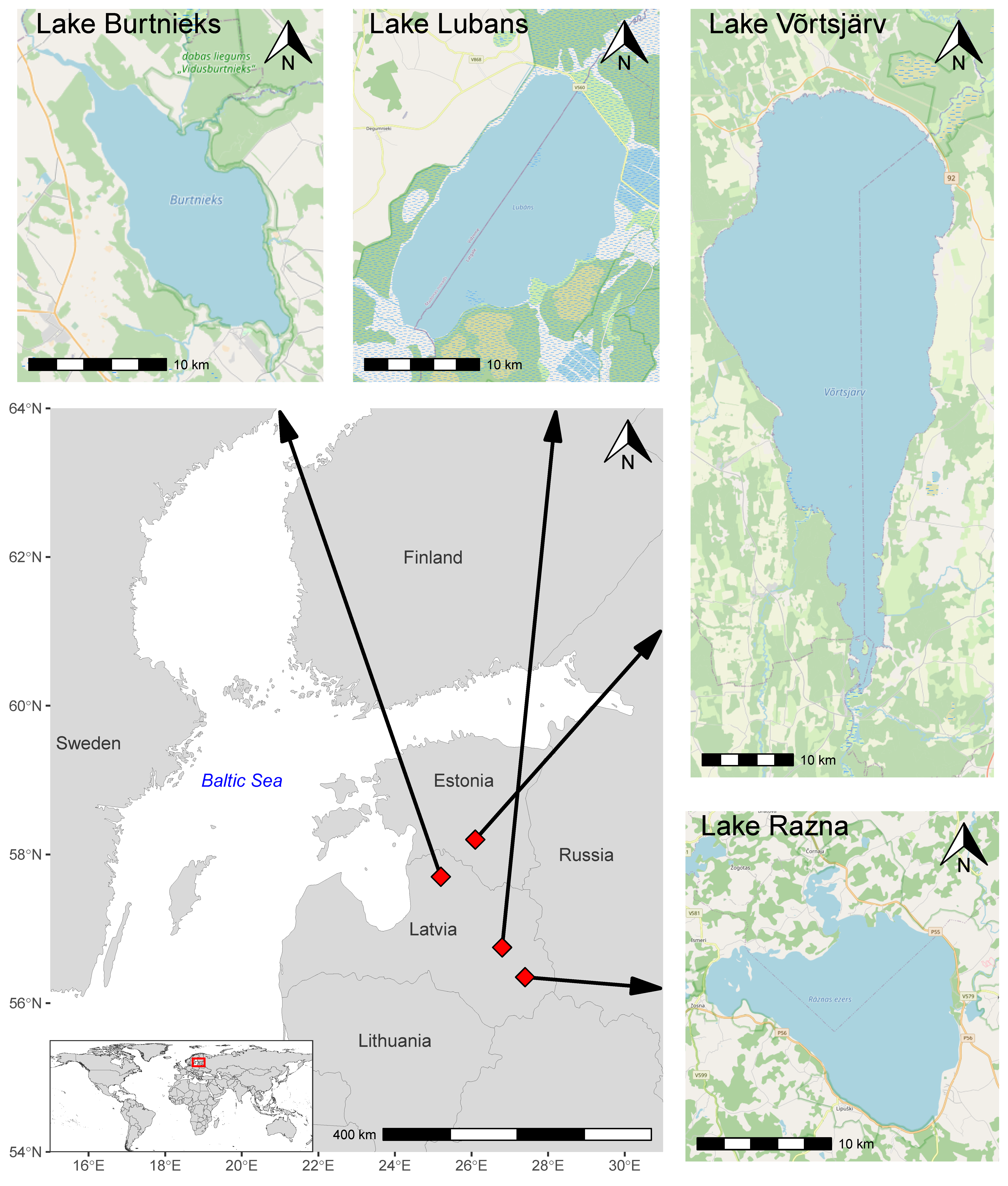
2.1. Study Sites

The study area included three Latvian and one Estonian lake, all of which are located in the northern boreal zone. The locations of the lakes are shown in Figure 1, and their geographical characteristics are shown in

Table 1. Characteristics of the lakes under investigation.

Lake	Location	Area, km2	Altitude, m	Mean Depth, m	Catchment Area, km2	Trophic State
Razna	56°19′N 27°28′E	57.6	164	7.0	229	mesotrophic
Lubans	56°46′N 26°52′E	80.7	90.0	1.6	2040	eutrophic
Võrtsjärv	58°16′N 26°02′E	270	33.7	2.8	3374	eutrophic
Burtnieks	57°44′N 25°14′E	40.2	47.0	2.4	2215	eutrophic

.

Lake Razna is located in the Latgale highlands in Latvia and has a surface area of 57.6 km² and catchment area of 229 km². It is the country’s second-largest lake by surface area and the largest by water volume (0.46 km³). According to the national monitoring database, Lake Razna is classified as a shallow lake with clear water [53], although the maximum depth reaches 17 m (mean depth of 7.0 m). The lake is mesotrophic; the Secchi depth (SD) was measured from 3.2 to 6.6 m (median 5.5 m) and Chl a from 1.4 to 10.9 mg m⁻³ (median of 6.4 mg m⁻³) during April to October 2018 [37].

Lake Lubans is situated in the center of the Eastern Latvian Lowland. The catchment area of the lake is 2040 km². At a water level of 90 m above sea level, the surface area of the lake is 80.7 km². However, the surface area of the lake can fluctuate from 25 to 100 km² due to an artificially regulated water level [54]. Lake Lubans is classified as a very shallow lake [53], where the maximum depth is 3.5 m and a the mean depth is 1.6 m. The lake is eutrophic and macrophyte-dominated; the SD was measured at 0.4–1.2 m (median of 0.9 m) and Chl a at 8.6–63.1 mg m⁻³ (median of 16.8 mg m⁻³) during April to October 2018 [37].

The large Lake Võrtsjärv (surface area of 270 km²) is in the central part of Estonia. It is the country´s second-largest lake, with a catchment area of 3374 km². Lake Võrtsjärv is also a shallow lake, with a maximum depth of 6.0 m (mean depth of 2.8 m). The unregulated water level can fluctuate annually up to 3.2 m (mean 1.4 m) [55]. In this eutrophic lake, the SD varied between 0.5 and 1.0 m (median of 0.6 m) and Chl a varied between 22.2 and 63.8 mg m⁻³ (median 33.1 mg m⁻³) during April to October 2018 [37].

Lake Burtnieks is situated in the northern part of Latvia. It is the fourth-largest lake in Latvia, with a surface area of 40.2 km² and a catchment area of 2215 km². Lake Burtnieks is a shallow eutrophic lake with a maximum depth of 4.3 m (mean depth of 2.4 m). The lake has brown water, where the SD was measured 0.4–1.2 m (median of 1 m) and Chl a at 6.7–117.1 mg m⁻³ (median of 19.1 mg m⁻³) during April to October 2018 [37].

2.2. Satellite Data

Cloud-free or partially cloud-free OLCI Level-1 full resolution images from onboard the Sentinel-3A and -3B satellites in 2018 were used in this study. Images were downloaded from the Copernicus Online Data Access platform [56] and processed with the atmospheric correction processor Case 2 Regional Coast Color (C2RCC) (v1) [57] using Sentinel Application Platform (SNAP) (v6) software developed by Brockmann Consult, SkyWatch, and C-S [58].

The retrieval of the water-leaving reflectance from OLCI Level-1 images involved three-step processing: (1) subsetting the case study lake from the entire scene using shape files of each lake; (2) applying the multisensor pixel identification tool (IdePix) and using in further analysis only the cloud-free inland water pixels by excluding pixels flagged as IDEPIX_CLOUD, IDEPIX_CLOUD_AMBIGUOUS, IDEPIX_CLOUD_SURE, IDEPIX_CLOUD_BUFFER, or IDEPIX_CLOUD_SHADOW; and (3) applying a C2RCC atmospheric correction processor using default parameters (except for temperature, which was set as 15 °C, and for salinity, which was set as 0.001 PSU) and excluding from further analysis pixels that were flagged as Kd489_OOR (K_d,489 product is out of range) or Cloud_risk. Only the images with ≥50% of the valid lake pixels were included in the further analysis.

Since standard remote sensing Chl a and K_d products often fail [59,60,61,62] in these optically complex inland waters, an alternative solution suggested for this region was used (detailed explanation are in Section 2.4.1 and Section 2.4.2).

2.3. The Primary Production (PP) Model

The PP model, originally developed by Arst et al. [20,52] and further adapted for remote sensing data by Kauer et al. [41] and Soomets et al. [42] was used in this study. The main principle of this model is that the PP is a function of photosynthetically absorbed radiation and the quantum yield of carbon fixation [63]:

$$\mathrm{PP}\left(z\right)=\Psi ·Q_{\mathrm{PAR}}^{*}\left(z\right)·F_{\mathrm{PAR}}\left(z\right)$$

(1)

where PP(z) is production in mg C m⁻³ h⁻¹ at depth z, Ψ is the factor 12 000 for converting moles of carbon to milligrams of carbon, Q^*_PAR(z) is photosynthetically absorbed radiation at depth z determined on the basis of scalar quantum irradiance (in mol photons m⁻³ h⁻¹), and F_PAR(z) is the quantum yield of carbon fixation (mol C (mol photons)⁻¹) in the PAR at depth z. The PP model has three input parameters: (1) Chl a in mg m⁻³, (2) K_d,PAR in m⁻¹, and (3) q_PAR in mol photons m⁻² h⁻¹. In this study, we followed the calculation scheme of the PP model modified for remote sensing data by Soomets et al. [42], and we used the integrated values of primary production (PP_int, mg C m⁻² h⁻¹) by integrating PP(z) over the mean depth of the lake for all valid pixels.

Based on the PP_int of the model, the following further calculations were made:

• The total lake PP_int (PP_lake, mg C h⁻¹) for the entire lake. As all available images with ≥50% of the valid lake pixels were used in the study, PP_lake was calculated by summarizing the available pixel values of PP_int, and then the average of the available pixels of a given day was taken to substitute all of the missing surface-area pixels.
• The average areal PP_int of the lake (PP_aver, mg C m⁻² h⁻¹) was taken as the average of the PP_lake over the surface area of the lake. For this parameter we also calculated the standard deviation (±) over the study period (April–October).
• The daily PP_lake (PP_lake,day, mg C d⁻¹) was calculated by multiplying PP_lake, the photoperiod (in h) of a given day, and the coefficient of 0.75 to take into account a daily light curve.
• The average daily areal PP_int for the entire lake (PP_day, mg C m⁻² d⁻¹) was taken as the average of the PP_lake,day over the surface area of the lake.
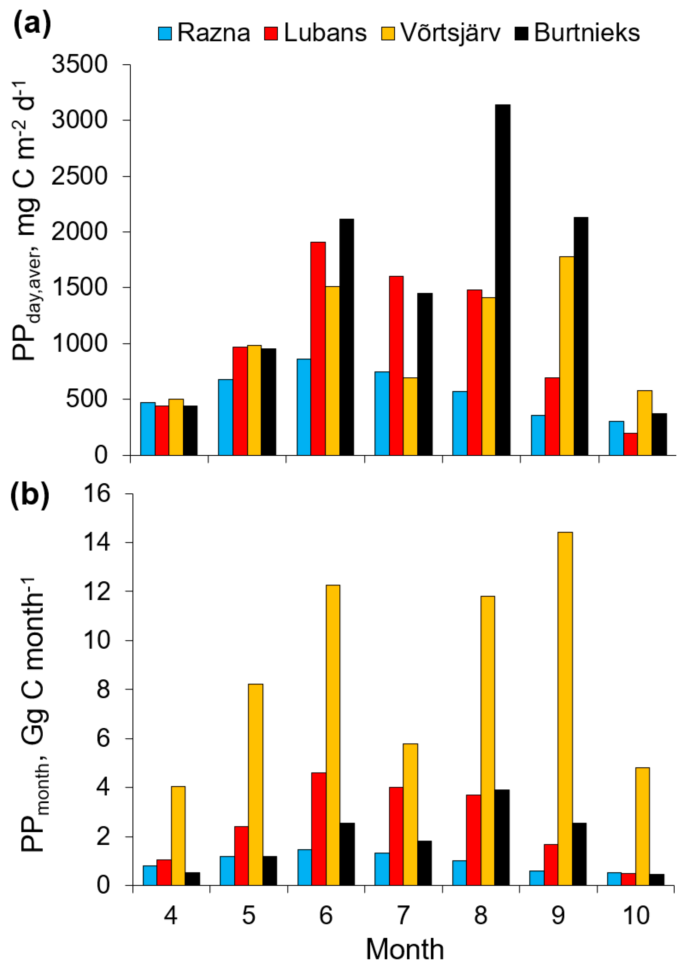
• The monthly average PP_day (PP_day,aver, mg C m⁻² d⁻¹) was taken as the average of the PP_day during one month.
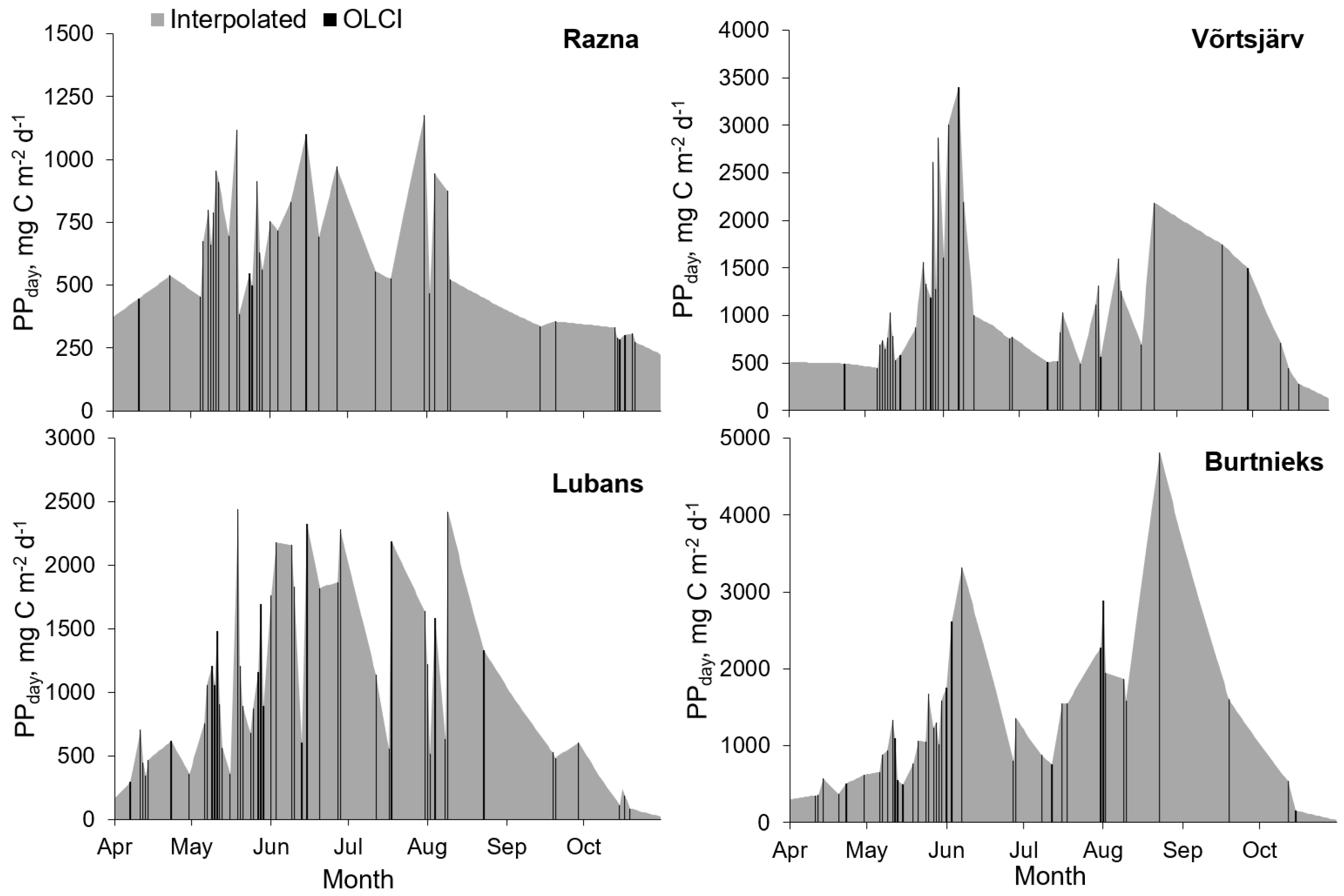
• The monthly productivity estimates of the entire lake (PP_month, Gg C month⁻¹) were taken as the sums of PP_lake,day for each month during the study period. If the PP_lake,day value was missing due to the absence of overpass of the satellite or cloudy conditions, then inter- or extrapolation was used to calculate missing the PP_lake,day value.
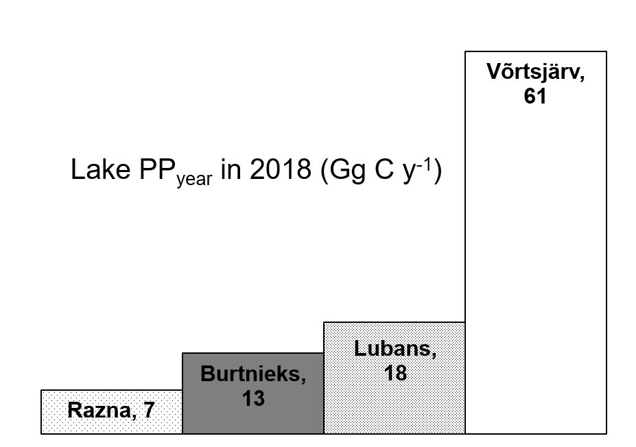
• The annual productivity estimates of the entire lake (PP_year, Gg C year⁻¹) were taken as the sums of PP_month during April–October 2018. We assumed that the PP during the rest of the months during 2018 is zero or close to zero due to ice and snow cover and not significant for the annual estimation of PP. Besides, there were no cloud-, ice-, or snow-free images available for the studied area from January to March, and November to December 2018.
• The annual average daily areal productivity (PP_year,aver, mg C m⁻² d⁻¹) was calculated by dividing PP_year by the number of days in a year and the surface area of the lake.

2.4. Input Parameters of the PP Model

The PP model has three input parameters: Chl a, K_d,PAR, and q_PAR. To study the seasonal and spatial variatios of PP in lakes, we used OLCI data for Chl a and K_d,PAR and in situ data for q_PAR for the PP model. The details of each input are described below.

2.4.1. Chlorophyll-a Concentration (Chl a)

For Chl a, the OWT guided approach by Soomets et al. [37] was used to retrieve Chl a values from OLCI water-leaving reflectance spectra. Classification of OWTs by Uudeberg et al. [64] divides boreal region inland and coastal water into five OWTs: (1) Clear OWT corresponds to waters with low OSC concentrations and high water transparency; (2) Moderate OWT corresponds to slightly higher OSC concentrations, but none of them dominate; (3) Turbid OWT corresponds to waters where TSM dominates; (4) Very Turbid OWT corresponds to waters where Chl a dominates, and it is associated with phytoplankton blooms; and (5) Brown OWT corresponds to waters where the CDOM dominates. The pixel was marked as “Unclassified” and excluded from further analyses if the reflectance spectrum of the pixel was “abnormal” in the blue part due to strong influence from sources other than water.

The OWT guided approach to retrieve Chl a values means that firstly, OWT is assigned to every valid OLCI image water pixel using a method by Uudeberg et al. [64]; and secondly, the most suitable algorithm developed by Soomets et al. [65] for each OWT is applied according to the pixel’s OWT. The Chl a algorithm used for each OWT is shown in Equation (2):

$$\mathrm{Chl}a=\{\begin{array}{cc}\hfill 44.75\ast \left(R_{TOA,709}/R_{TOA,674}\right)-32.78,& \mathrm{OWT}=\mathrm{Clear}\hfill \\ \hfill -21601\ast (\left(R_{TOA,665}-R_{TOA,709}\right)*R_{TOA,754})+23.78,& \mathrm{OWT}=\mathrm{Moderate}\hfill \\ \hfill 1552.3\ast (R_{TOA,709}-\left(R_{TOA,665}+R_{TOA,754}\right)/2)+21.03,& \mathrm{OWT}=\mathrm{Turbid}\hfill \\ \hfill -246.33\ast \left(R_{TOA,665}/R_{TOA,709}\right)+291.75,& \mathrm{OWT}=\mathrm{Very\; Turbid}\hfill \\ \hfill -316.56\ast \left(R_{TOA,665}/R_{TOA,709}\right)+365.88,& \mathrm{OWT}=\mathrm{Brown}\hfill \end{array},$$

(2)

where R_TOA,x is the OLCI top-of-atmosphere reflectance at the specific band that is labeled with its central wavelength.

2.4.2. The Underwater Light Diffuse Attenuation Coefficient (K_d,PAR)

For K_d,PAR, the calculations from OLCI image data consisted of two main steps. Firstly, the underwater light diffuse attenuation coefficient at 490 nm (K_d,490) was calculated from water-leaving reflectance spectra using weighted band ratio algorithms by Alikas et al. [66]:

$$K_{\mathrm{d},490}=\left(1-W\right)·K_{\mathrm{d},490,\left(\frac{490}{709}\right)}+W·K_{\mathrm{d},490,\left(\frac{560}{709}\right)},$$

(3)

where W is a calculated weight that is used to combine the two separate K_d,490 algorithms. It is calculated according to Equation (4):

$$W=5.098-2.2099·\frac{R_{560}}{R_{709}}\begin{array}{cc}for& \hspace{1em}1.519\le \end{array}\frac{R_{560}}{R_{709}}\le 1.796,$$

(4)

where R₅₆₀ and R₇₀₉ are the OLCI water-leaving reflectance values on specific bands.

The two K_d,490 algorithms from Equation (3) are calculated using Equation (5):

$$K_{\mathrm{d},490,\left(\frac{R_{\lambda 1}}{R_{\lambda 2}}\right)}=K_{w,490}+A·{\left(\frac{R_{\lambda 1}}{R_{\lambda 2}}\right)}^B,$$

(5)

where R_λ1 and R_λ2 mark the water-leaving reflectance values on specific OLCI bands (490, 560, or 709 nm). K_w,490 is the pure water light attenuation coefficient at 490 nm and is 0.016 m⁻¹; A and B are coefficients derived by linear regression analysis for the band ratio algorithms: −0.9461 and 0.4305 for $K_{\mathrm{d},490,\left(\frac{490}{709}\right)}$, and −1.1198 and 1.4141 for $K_{\mathrm{d},490,\left(\frac{560}{709}\right)}$.

Secondly, we converted K_d,490 to K_d,PAR using Equation (6):

$$K_{\mathrm{d},\mathrm{PAR}}=0.4349·K_{\mathrm{d},490}+0.3291.$$

(6)

2.4.3. Incident Planar Downwelling Irradiance (q_PAR)

The hourly average diffused sky irradiance for PAR (in µmol m⁻² s⁻¹) was measured in situ with the SkySpec spectroradiometer [67] at the Station for Measuring Ecosystem–Atmosphere Relations, SMEAR-Estonia, a research station in Järvselja, Estonia (58°16′40.60″N, 27°18′30.84″E), during 2018. For the PP model q_PAR input, we used the measured daily maximum values converted to mol photons m⁻² h⁻¹ for each day we had OLCI data. We used the same maximum daily q_PAR values for all of the studied lakes because they are located close enough to each other (the maximum distance from the station to the lake was about 220 km).

3. Results

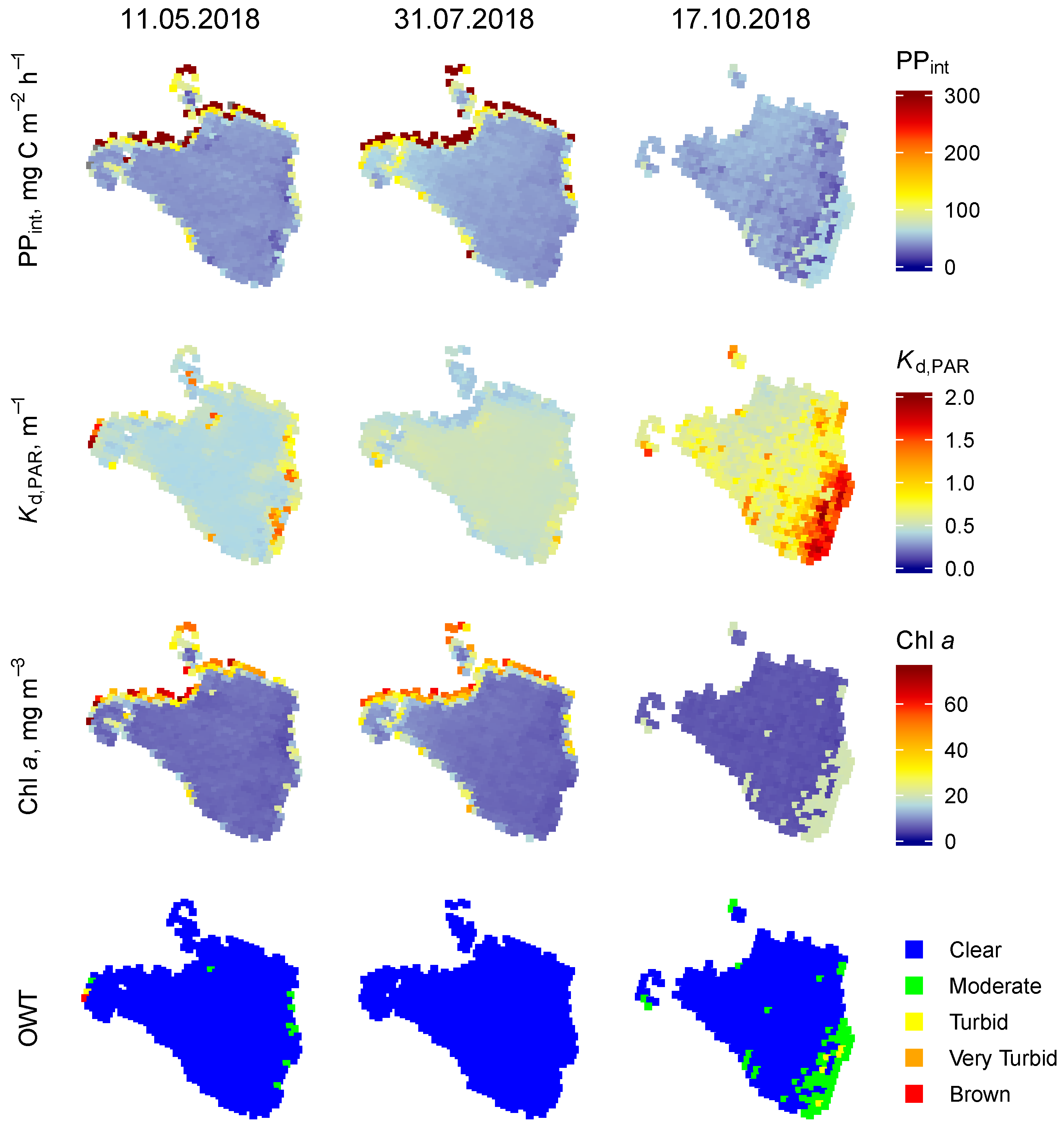
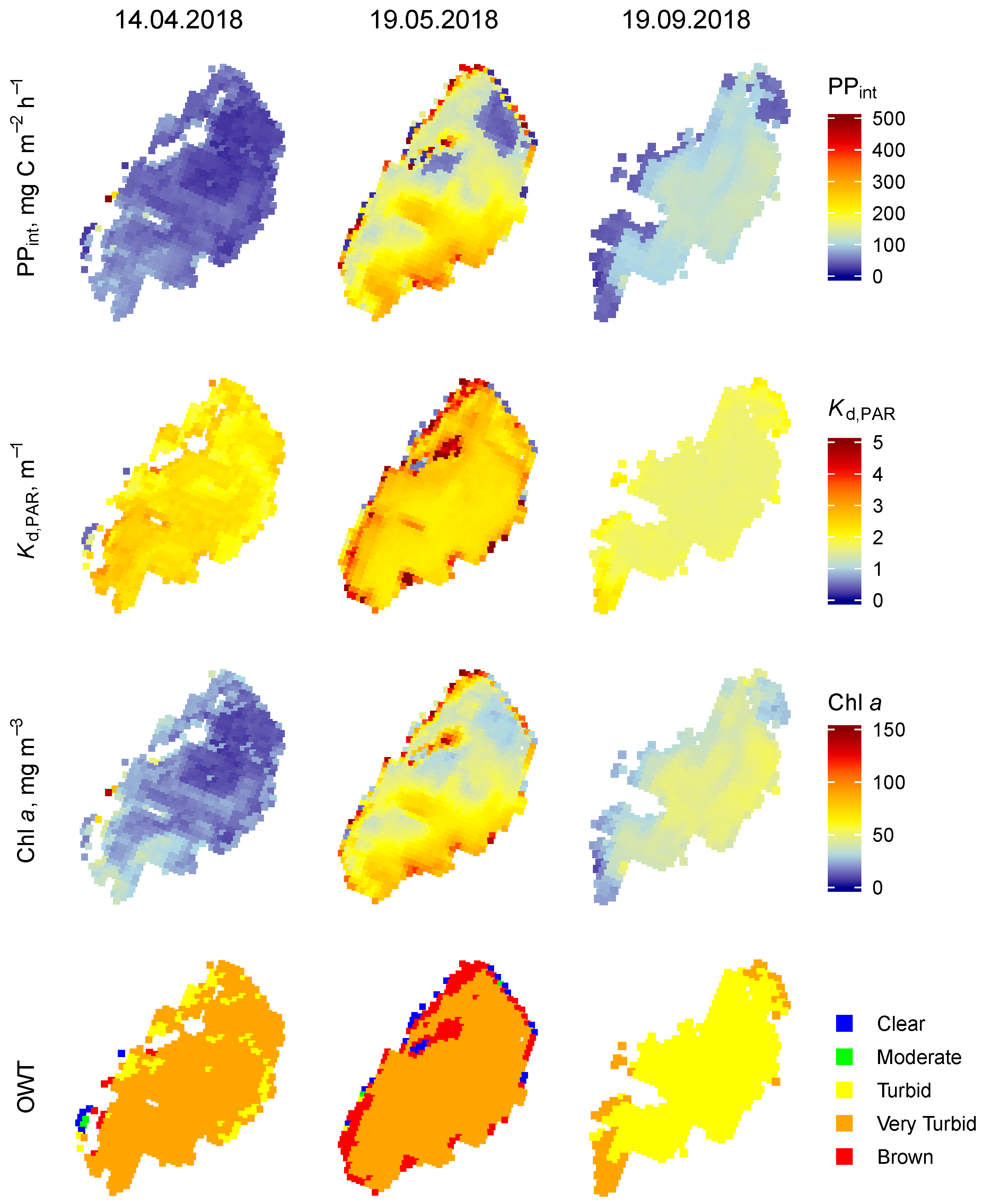
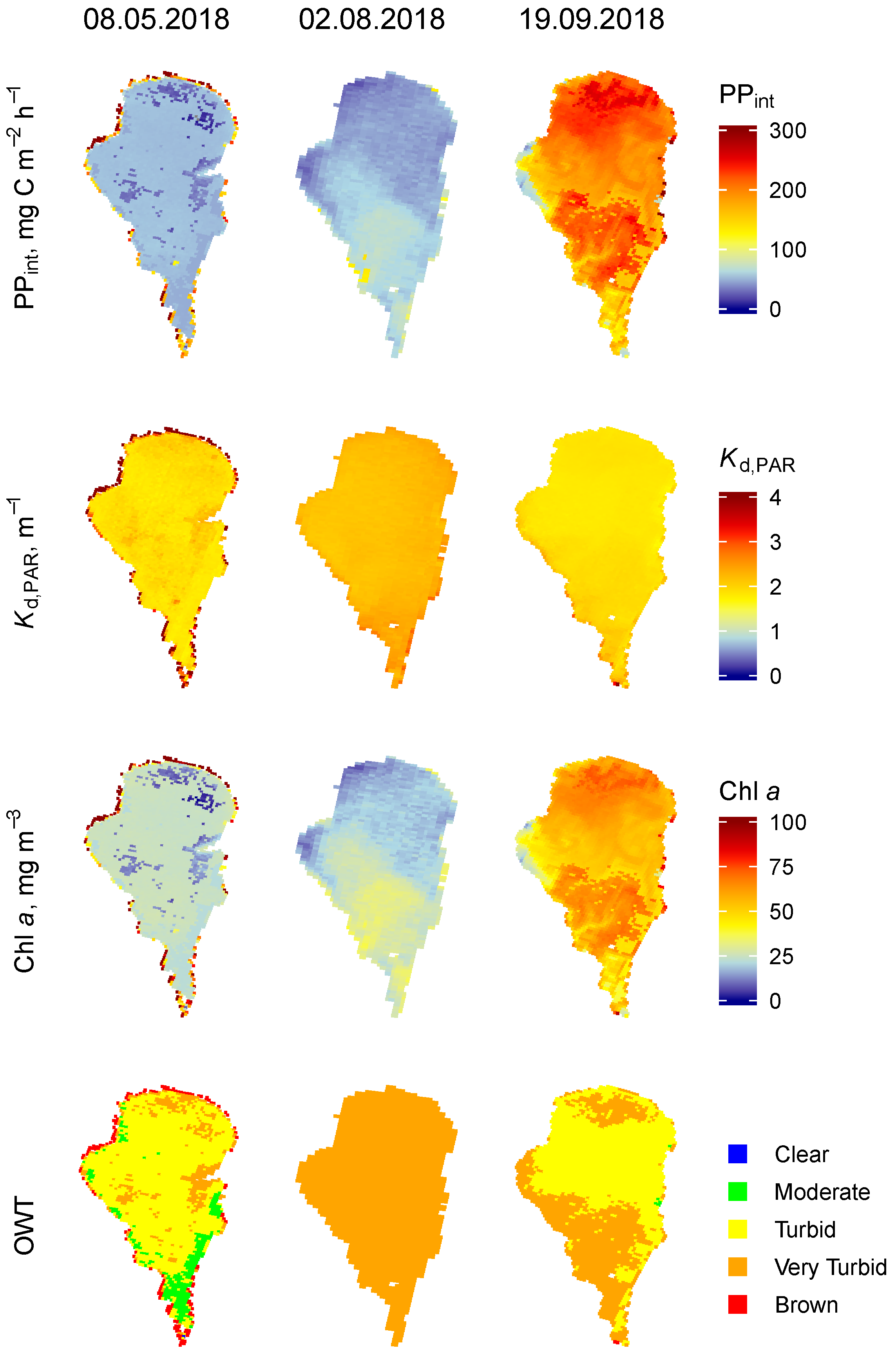
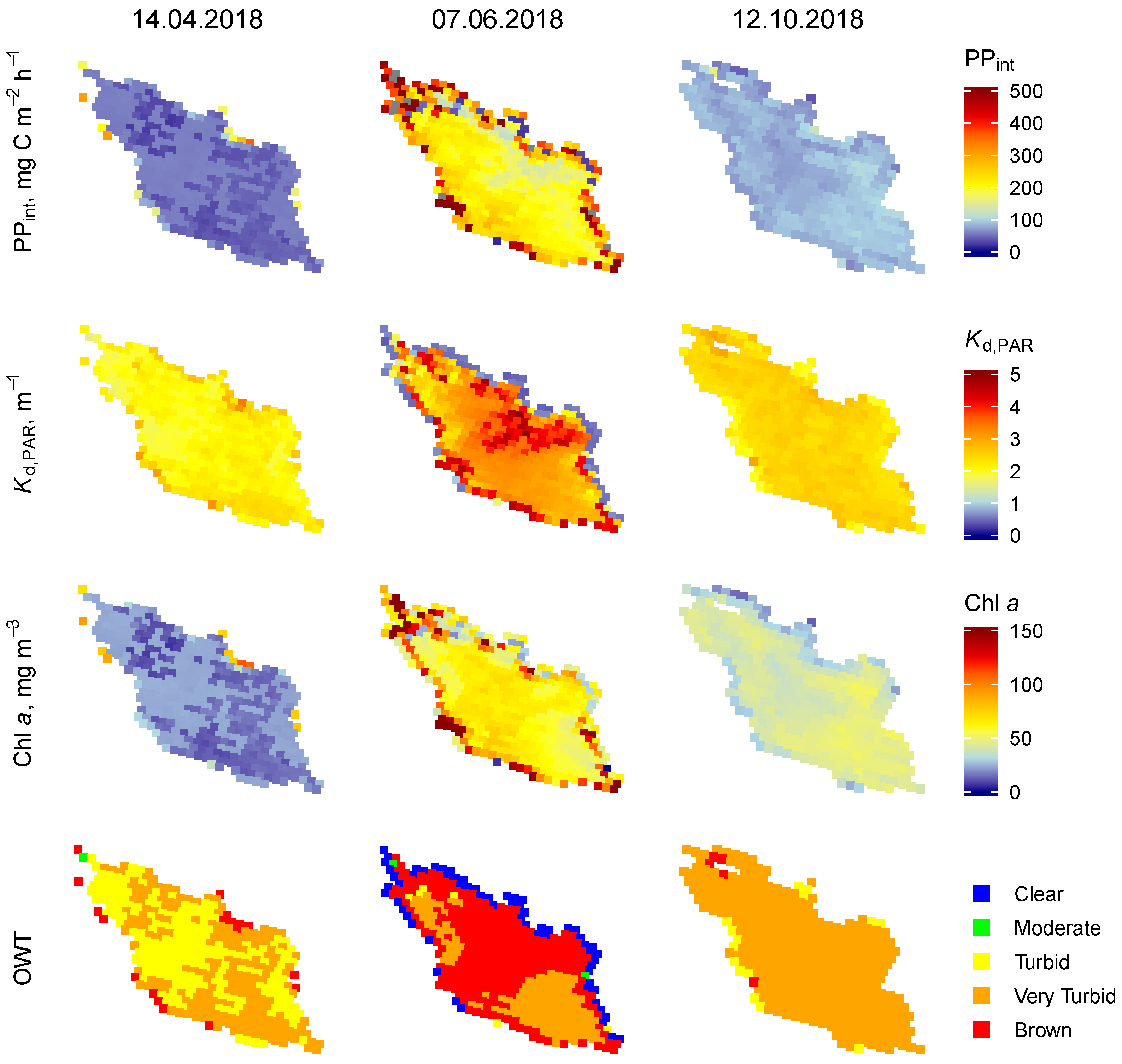
3.1. Spatial Variability of PP

The spatial variability of PP_int during 2018 was studied via derived PP_int spatial variability maps from OLCI cloud-free or partially cloud-free images; altogether (for all four lakes), we generated 161 PP_int spatial maps (approximately 40 for each studied lake). The used PP model has three input parameters, of which two were spatiality variables: Chl a and K_d,PAR. Since Chl a was determined using the OWT guided approach, the examples of the resulting PP_int (mg C m⁻² h⁻¹) together with the derived inputs of the PP model, K_d,PAR, Chl a, and OWT, are shown in Figure 2, Figure 3, Figure 4 and Figure 5.

3.1.1. Lake Razna

The clear water Lake Razna showed little spatial variability in its PP_int. In spring and summer, the likelihood of higher PP_int was at the northern shoreline of the lake (Figure 2). However, slightly higher productivity in the southern part was often present in autumn. The Clear OWT was very dominant in Lake Razna, and a majority of the pixels had low Chl a (mean 11.1 ± 17.3 mg m⁻³) and K_d,PAR (mean 0.62 ± 0.57 m⁻¹) values; therefore, the productivity of the lake was also low. The PP_aver over the study period was 51.2 ± 14.9 mg C m⁻² h⁻¹.

3.1.2. Lake Lubans

The eutrophic Lake Lubans showed high spatial variability in its bio-optical characteristics; the waters were classified mostly Turbid and Very Turbid throughout the study period. A very distinguishing pattern for Lake Lubans was the decrease of the open water area during vegetation season due to the growing vegetation. This was clearly seen in late August and September, where the open-water area was diminished markedly (Figure 3, 19 September 2018). The mean Chl a was 42.4 ± 40.0 mg m⁻³, with a much lower median value (29.4 mg m⁻³), and the mean K_d,PAR was 2.52 ± 1.08 m⁻¹. The PP_aver over the study period was 90.9 ± 53.9 mg C m⁻² h⁻¹.

3.1.3. Lake Võrtsjärv

The largest of the studied Lake Võrtsjärv also showed a relatively high spatial variability of PP_int. The PP_int was often higher in the southern part of the lake, and in some cases, the inflow of a river to the lake was clearly visible in the southwestern part, where the PP_int values are slightly lower than in the surrounding waters (Figure 4, 19 September 2018). The dominant OWT was either Turbid or Very Turbid. The mean Chl a was 33.4 ± 20.4 mg m⁻³ but was much higher in the bloom condition (Figure 4), and the mean K_d,PAR was 2.15 ± 0.55 m⁻¹. The PP_aver over the study period was similar to Lake Lubans: 100.0 ± 65.1 mg C m⁻² h⁻¹.

3.1.4. Lake Burtnieks

The smallest and the brownest water lake of the current study showed the highest variability in all of the bio-optical characteristics and PP_int. Higher productivity of the entire lake was shown especially in late summer. Often, there is a distinct shoreline of higher productivity around the lake (Figure 5). The dominant OWT was either Turbid, Very Turbid, or Brown, but the Moderate OWT was also frequently present. The mean Chl a was 43.5 ± 37.3 mg m⁻³, with a much lower median value (27.7 mg m⁻³), and the mean K_d,PAR was 2.58 ± 1.02 m⁻¹. The PP_aver over the study period was 139.2 ± 108.6 mg C m⁻² h⁻¹.

3.2. Temporal Variability of the PP

We calculated the average daily areal production (PP_day) and the total daily production of the lake (PP_lake,day) from the OLCI data for the entire lake. For the dates that we did not have OLCI data, we interpolated (or extrapolated to April 1 and October 31 to get full months) the modelled PP_lake,day values. In the period of April to October, we had about 40 days of satellite data (Razna 38, Burtnieks 40, Lubans 42, Võrtsjärv 41), but the satellite data was not distributed equally. The highest number of cloud-free images was acquired in May, whereas in September and October, we had only a few images to use. From November to April, we either did not have any cloud-free images or the lakes were ice-covered. The temporal variability of the PP_day shows different patterns for each lake (Figure 6).

In Lake Võrtsjärv and Lake Burtnieks, the PP_day showed a clear two-peak pattern over the vegetation period. The first productivity peak was in late spring/early summer (first half of June), and the second productivity rise was in late summer (end of August and September) (Figure 6). The main difference in the seasonal pattern of those lakes was the duration of the second production peak. In Lake Võrtsjärv, the late summer peak lasted longer (1.5 months) and was not as intense as the spring one. In Lake Burtnieks, both productivity peaks lasted about 3 weeks and the second peak was more intense (Figure 6).

The temporal variability of the PP_day had rather similar patterns in Lake Razna and Lubans: both of those lakes are missing the summer “clear” period between the two high productivity periods. Although in Lake Razna, the maximum productivity occurred in early summer, while in Lake Lubans it was in late summer (Figure 6).

Another very characteristic feature of Lake Burtnieks was the large range of PP_day values. For example, the range of PP_day was over 4600 mg C m⁻² d⁻¹ for the study period, being 4817 mg C m⁻² day⁻¹ on 23/08/2018 and 156 mg C m⁻² d⁻¹ on 15/10/2018. Other lakes showed much smaller ranges of PP_day, with Lake Razna having the smallest range of 950 mg C m⁻² d⁻¹. Lake Razna also had the lowest maximum PP_day values (1177 mg C m⁻² d⁻¹), while in Lake Burtnieks it was 4 times higher.

To compare the monthly productivity of the studied lakes, we calculated the monthly averages for PP_day (PP_day,aver) (Figure 7a). Here, as before, Lake Burtnieks had the highest production rates, but only for the three peak-productivity months (June and August–September). The temporal variability of the PP_day,aver in different lakes was demonstrated again, with Lake Lubans having the highest PP_day,aver in July, when Lake Võrtsjärv and Lake Burtnieks had a lower PP_day,aver (Figure 7a).

Another estimate that we compared between the lakes was the total monthly productivity for the entire lake (PP_month). The PP_month showed vast differences in lakes. It varied from 0.46 Gg C month⁻¹ (Burtnieks, October) to 14.4 Gg C month⁻¹ (Võrtsjärv, September) (Figure 7b). Here, the impact of lake size on the overall productivity is clearly shown. For example, in August, even though Lake Burtnieks showed twice the production rate per area unit compared with Lake Võrtsjärv (3137 and 1411 mg C m⁻² d⁻¹, respectively), the total production of Lake Burtnieks for this month was 3.9 Gg C month⁻¹ whilst for Lake Võrtsjärv, which is more than six times larger, it was three times higher (11.8 Gg C month⁻¹) (Figure 7).

Lake size plays an important role also in the yearly lake productivity. For the yearly production, we added the monthly sums of lake production from April to October. We assumed that the production from November to March was not significant [68]. The yearly production of 2018 for the entire lake varied from 7 Gg C y⁻¹ (Razna) to 61 Gg C y⁻¹ (Võrtsjärv) (Figure 8).

As we assumed the productivity to be zero or close to that for 5 months of the year, the annual average daily areal productivity (PP_year,aver) in Lake Razna would be 333.0 mg C m⁻² d⁻¹, in Lake Burtnieks, 887.3 mg C m⁻² d⁻¹, in Lake Lubans, 610.2 mg C m⁻² d⁻¹, and in Lake Võrtsjärv, 622.4 mg C m⁻² d⁻¹. This shows that the most productive was the smallest of our studied lakes. Lake Võrtsjärv and Lake Lubans show very similar PP_year,aver, although the total productivity of the lakes was very different.

4. Discussion

To estimate the spatial and temporal variability of PP, we used 161 cloud-free OLCI scenes over four different Baltic lakes during 2018. The OLCI images were processed with a C2RCC atmospheric processor, and to determine the PP model inputs Chl a and K_d,PAR from the reflectance spectra of each pixel, the OWT guided approach for Chl a and the weighted band ratio algorithms method for K_d,PAR was used. The PP_day was calculated to estimate the temporal variability. Finally, daily, monthly, and yearly PP_int estimates for each lake were determined.

The spatial variability of PP_int in Lake Razna showed the presence of phytoplankton blooms on the northern shores of the lake (Figure 2) during spring; this pattern is also shown as the PP_day peaks in the temporal variability (Figure 6). In the autumn, the PP_int had higher values in the southeastern part compared to the rest of the lake on some days, likely because of the winds that would drive the phytoplankton to the shoreline area. The PP_day,aver values of this mesotrophic lake are quite similar to the other studied (eutrophic) lakes in April (Figure 7a) because Lake Razna is significantly deeper than the other lakes; therefore, the PP_int values, which are calculated by integration over the mean depth of the lake, are also higher.

Although Kauer et al. [69] demonstrated that the PP_day values can significantly vary from day to day due to the changing climate condition; the rapid fluctuations of PP_day in the current work are mostly caused by the different number of pixels used for a specific day. As we had the requirement that at least 50% of the lake pixels should be valid, it sometimes resulted that the parts of the lake with higher productivity were filtered out (due to the clouds) and the clear water pixels with low PP values were used to estimate PP_day. This phenomenon was more pronounced in Lake Razna and Lake Lubans, where flagging out part of the pixels had larger impact on the PP_day estimates due to the PP_int spatial variation. In addition to the missing pixels, there were errors in the atmospheric correction when thin cirrus clouds or other fine atmospheric particles were not correctly flagged out by used processors.

In this study, the assumption was made that the lake-bottom influence is negligible in our PP estimations, and no additional corrections were applied to remove the bottom influence from the remote sensing signal due to the lakes water mainly being optically deep waters. In Lake Lubans, Burtnieks, and Võrtsjärv, the water transparency (SD ≤ 1.2 m) is lower than the average depth (1.6 m, 2.4 m, and 2.8 m, respectively; Table 1); therefore, lake bottoms were not visible from the water surface and were not influencing the reflectance spectra. A lake’s bottom can be visible up to few meters from the shore; however, the OLCI pixel size is 300 m. In the clear water Lake Razna, the situation was handled more carefully. Since water transparency in Lake Razna was high (SD was up to 6.6 m) and the sandy bottom was visible in the east side of the lake (depth up to 6 m), we investigated the bottom’s influence before making this assumption. The reflectance spectra retrieved in lake areas where the bottom was visible acted similarly to that described by Vahtmäe et al. [70]. Nevertheless, in our case, the bottom influence was not strong enough to change the optical water type or the retrieval of Chl a. However, the bottom influence was slightly shown in the retrieved K_d product. But since the PP model used in this study is more sensitive to Chl a than K_d in clear water cases, the bottom influence is not detectable in the PP_int results.

Overall, the PP_day results were quite high for Lake Lubans throughout the summer, without having clear PP_day peaks as in Lake Burtnieks (Figure 6). Due to extremely high PP_day peaks in Lake Burtnieks, the PP_aver was also about 30% higher than in Lake Võrtsjärv and Lake Lubans. The higher PP_int values in the shore areas are quite usual in all of the lakes, but the most prominent is in Lake Burtnieks, caused by the shallower, more nutrient-rich waters. Another possible reason for higher values in the shore area is an adjacency effect—bias in the spectral signal due to perturbations by the radiance reflected by the land, which are propagated by the atmosphere into the satellite sensor [71].

In the case of Lake Burtnieks and Lake Lubans, Clear OWT is shown along the shorelines of the lakes, which is likely the result of the atmospheric correction issues due to processing with C2RCC [64,72]. For example, the atmospheric correction has been proven to be complicated in the case of dark water (Brown OWT), with the blue part of the spectrum being strongly overestimated. This can cause false classification to the Clear OWT [64,73]. Another cause could be the effect of the in-water vegetation on the reflectance spectra that leads to misclassification of the pixel. The insufficient quality flagging of the C2RCC and/or poor clear water pixel masking by the IdePix tool can also cause a situation where these pixels are falsely classified as clear water pixels [3]. However, the added extra quality flag (Kd489_OOR) seems to exclude most of the pixels affected by the in-water vegetation for Lake Lubans. Thus, the two lakes have a different source for the OWT misclassification: for Lake Lubans, the cause is the in-water vegetation, and for Lake Burtnieks, the brown water. Despite the issues addressed above, our OWT classification results for 2018 generally agree with the previous study for 2017 [72].

Lake Võrtsjärv typically had higher PP_int in the southern part of the lake (Figure 4), which is narrower and has different optical properties than the open northern part. Nõges et al. [68] used modeling to reconstruct a long time-series of the areal productivity in Lake Võrtsjärv. They obtained 10% lower PP_year,aver results than the current study: 558 mg C m⁻² d⁻¹. One of the probable causes of this difference could be the different lengths of the study periods: the current study was focused only on the year 2018, but the result of Nõges et al. [68] is the mean productivity value over 27 years. Also, our results regarding the PP_day,aver (Figure 7a) largely agree with Nõges et al. [68]. Their Figure 4 shows similar monthly values, except for September, where the PP_day,aver is almost three times lower. This difference might be explained by the yearly differences in weather conditions. Although the September PP_day,aver values were mostly around 600–1000 mg C m⁻² d⁻¹ for the years 1982–2009, it was approximately 2000 mg C m⁻² d⁻¹ in 2006 (Nõges et al. [68] Figure 6), which is a bit higher than the our estimation for September 2018 (1780 mg C m⁻² d⁻¹, Figure 7a).

There have been large discrepancies in the PP results obtained in different studies using different methods. The long-term study (1982–2009) by Nõges et al. [68] estimated the average PP from June to October to be 880 mg C m⁻² d⁻¹, based on ¹⁴C methods, while another study [19] estimated the PP from oxygen measurements to be 1632 mg C m⁻² d⁻¹ (June to October 2011–2012). Our results would be placed in the middle of those two past studies, with the PP estimated to be 1188 mg C m⁻² d⁻¹ from June to October 2018. Our calculations are based on the mean of the entire lake, while the two past studies made their estimations based on measurements from a single point.

PP studies in lakes using remote sensing data have not been very abundant so far. The Great Lakes Primary Productivity Model (inputs are Chl a, K_d,490, q_PAR, and also the photosynthesis-irradiance index) to study PP in the Great Lakes (Superior, Huron, and Michigan) using satellite data has been applied in multiple studies [33,74,75]. These already showed promising results of spatiotemporal PP studies and stated the advantages of PP modeling with satellite data. A similar model was applied to remote sensing data by Bergamino et al. [76] to study Lake Tanganyika and Deng et al. [23] to study Lake Taihu. Lake Geneva has been also investigated with remote sensing data using the same model as in the current study [42].

Fahnenstiel et al. [33] estimated the PP_year in the Great Lakes to be 5300–8100 Gg C y⁻¹ (

Table 2. The comparison of different lakes by their surface area (S, km²), yearly total primary production (PP_year, Gg C y⁻¹), and annual average daily areal productivity (PP_year,aver, mg C m⁻² d⁻¹).

Lake	S (km2)	PPyear (Gg C y−1)	PPyear,aver (mg C m−2 d−1)	Reference
Superior	82,103	8100	274	[4]
Huron	59,590	5300	247	[4]
Michigan	58,030	6300	301	[4]
Tanganyika	32,900	7651 1	646	[76]
Taihu	2338	890	1094	[23]
Geneva	580	180	828	[42]
Võrtsjärv	270	61	622	Current study
Lubans	80.7	18	610	Current study
Burtnieks	40.2	13	887	Current study
Razna	57.6	7	333	Current study

¹ Units are converted by the authors of current study.

) [75]. Although the sizes of lakes Superior, Huron, or Michigan are not comparable to the smaller lakes targeted in the current study, the PP_year,aver showed, for example, that Lake Burtnieks can have more than threefold higher production per m² (Table 2). The lake size plays an important role in the total lake productivity. It is clear that lakes with otherwise similar areal productivity (Lubans, Võrtsjärv, and Tanganyika) have very different PP_year, ranging from 18 to 7651 Gg C y⁻¹ (Table 2).

The oligo-mesotrophic Lake Geneva shows a higher PP_year,aver than eutrophic lakes Võrtsjärv and Lubans, but two factors should be kept in mind. Firstly, the PP_year,aver values are derived from the PP(z) values over the depth of the euphotic zone, where photosynthesis can occur. In Lake Geneva, the euphotic mixed layer zone can reach up to 30 m (according to Luhtala et al.’s [77] algorithm from the maximum measured SD [78]), while in shallow lakes like Lubans and Võrtsjärv, the euphotic zone cannot exceed the maximum depths of 3.5 m and 6 m, accordingly. Secondly, the lakes are exposed to different climate conditions: Lake Geneva does not have any ice cover. This allows higher production during the entire year, leading to a higher PP_year,aver. This might also be one of the reasons, besides the high amount of available nutrients, why Lake Taihu is seemingly the most productive lake, with the highest mean PP_year,aver (Table 2). Actually, in the highest productivity month, August, the PP_day,aver was 1675.5 ± 710.4 mg C m⁻² d⁻¹ [23] in Lake Taihu, whereas in Lake Burtnieks the PP_day,aver was 3137.6 ± 1105 mg C m⁻² d⁻¹ in August 2018 (Figure 7a).

Although initially it might seem from the Table 2 that smaller lakes would not contribute significantly to the carbon cycle, lakes with surface areas of 1–1000 km² cover about 36% (~1.9 million km²) of the total area of all lakes in the world [5]. Fee et al. [79] stated that the areal production is generally higher for medium-sized lakes, which have a combined offset of temperature and turbulence supporting increased phytoplankton growth, but larger lakes have higher yearly production due to a prolonged growing season. And yet, still a relatively small portion of smaller lakes are monitored regularly or not monitored at all, hence a large portion of the global freshwater productivity is not considered.

The method used in the current work could be easily applicable to larger regions to cover more lakes with different optical properties. The medium-resolution OLCI data where one pixel covers approximately 0.09 km² is only suitable for monitoring lakes with a diameter of more than 1 km, leaving the most abundant lake group out of its capability. In addition, although even OLCI data show some spatial patterns, data from high-resolution Sentinel-2 (pixel size from 10 × 10 m to 60 × 60 m, depending on the spectral band) might be even more useful for PP studies of smaller lakes and their spatial variability. This is an especially strong advantage in vegetation-rich lakes like Lubans, allowing the distinguishing of patches of vegetation with higher accuracy, whilst Sentinel-3 pixels are affected by vegetation and thus invalid. Also, Sentinel-2 is proven to have higher quality flagging than Sentinel-3 OLCI [37,72], hence the PP results can be improved. In addition, the PP estimation scheme developed in the current work could be applied to even larger regions and on a longer time scale for interannual comparisons. Even smaller lakes could be included with higher resolution remote sensing data, but in this case, the PP results of the shoreline pixels must be handled with some caution due to the possible influence of the bottom and the adjacency effect; therefore, some additional masks or methods might need to be applied.

5. Conclusions

The aim of this study was to estimate spatial and temporal PP variability in four lakes by using a PP model based on Sentinel-3 OLCI data. From our studied lakes, only one lake had previous records of PP (Lake Võrtsjärv). Soomets et al. [42] demonstrated that the model gives good results also in deep lakes with a mixed euphotic zone. Consequently, we can also apply the model to the mesotrophic and relatively deep Lake Razna similarly to three other shallow and eutrophic lakes, despite the model being designed for lakes with a well-mixed water column where K_d,PAR and Chl a do not change (or only change slightly) with depth [52]. The annual average daily areal productivity, PP_year,aver, in 2018 was 333 mg C m⁻² d⁻¹ in Lake Razna, 610.2 mg C m⁻² d⁻¹ in Lake Lubans, 622.4 mg C m⁻² d⁻¹ in Lake Võrtsjärv, and 887.3 mg C m⁻² d⁻¹ in Lake Burtnieks. This shows that the most productive lake is the smallest of the studied lakes. The yearly total production of 2018 for the entire lake was 7 Gg C y⁻¹ (Lake Razna), 13 Gg C y⁻¹ (Lake Burtnieks), 18 Gg C y⁻¹ (Lake Lubans), and 61 Gg C y⁻¹ (Lake Võrtsjärv). Even if lake size plays a significant role in the total PP of the lake, the abundance of small and medium-sized lakes would sum up to significant carbon fixation. Hopefully, the free access to Sentinel-2 high-resolution remote sensing data and improved methods will bring the freshwater PP more into the focus of the carbon cycle studies.

References

1. Hamilton, T.L.; Corman, J.R.; Havig, J.R. Carbon and nitrogen recycling during cyanoHABs in dreissenid-invaded and non-invaded US midwestern lakes and reservoirs. Hydrobiologia 2020, 847, 939–965. [Google Scholar] [CrossRef] [Green Version]
2. Huttunen, J.T.; Alm, J.; Liikanen, A.; Juutinen, S.; Larmola, T.; Hammar, T.; Silvola, J.; Martikainen, P.J. Fluxes of methane, carbon dioxide and nitrous oxide in boreal lakes and potential anthropogenic effects on the aquatic greenhouse gas emissions. Chemosphere 2003, 52, 609–621. [Google Scholar] [CrossRef]
3. Cole, J.J.; Prairie, Y.T.; Caraco, N.F.; McDowell, W.H.; Tranvik, L.J.; Striegl, R.G.; Duarte, C.M.; Kortelainen, P.; Downing, J.A.; Middelburg, J.J.; et al. Plumbing the Global Carbon Cycle: Integrating Inland Waters into the Terrestrial Carbon Budget. Ecosystems 2007, 10, 172–185. [Google Scholar] [CrossRef] [Green Version]
4. Sanches, L.F.; Guenet, B.; Marinho, C.C.; Barros, N.; de Assis Esteves, F. Global regulation of methane emission from natural lakes. Sci. Rep. 2019, 9, 255. [Google Scholar] [CrossRef] [PubMed] [Green Version]
5. Verpoorter, C.; Kutser, T.; Seekell, D.A.; Tranvik, L.J. A global inventory of lakes based on high-resolution satellite imagery. Geophys. Res. Lett. 2014, 41, 6396–6402. [Google Scholar] [CrossRef]
6. Tranvik, L.J.; Downing, J.A.; Cotner, J.B.; Loiselle, S.A.; Striegl, R.G.; Ballatore, T.J.; Dillon, P.; Finlay, K.; Fortino, K.; Knoll, L.B.; et al. Lakes and reservoirs as regulators of carbon cycling and climate. Limnol. Oceanogr. 2009, 54, 2298–2314. [Google Scholar] [CrossRef] [Green Version]
7. Klaus, M.; Seekell, D.A.; Lidberg, W.; Karlsson, J. Evaluations of Climate and Land Management Effects on Lake Carbon Cycling Need to Account for Temporal Variability in CO2 Concentrations. Global Biogeochem. Cycles 2019, 33, 243–265. [Google Scholar] [CrossRef] [Green Version]
8. Field, C.B. Primary Production of the Biosphere: Integrating Terrestrial and Oceanic Components. Science 1998, 281, 237–240. [Google Scholar] [CrossRef] [Green Version]
9. Marra, J. Vertical Mixing and Primary Production. In Primary Productivity in the Sea; Springer US: Boston, MA, USA, 1980; pp. 121–137. [Google Scholar]
10. Kimmel, B.L.; Groeger, A.W. Factors controlling primary production in lakes and reservoirs: A perspective. Lake Reserv. Manag. 1984, 1, 277–281. [Google Scholar] [CrossRef]
11. Downs, T.M.; Schallenberg, M.; Burns, C.W. Responses of lake phytoplankton to micronutrient enrichment: A study in two New Zealand lakes and an analysis of published data. Aquat. Sci. 2008, 70, 347–360. [Google Scholar] [CrossRef]
12. Sterner, R.W. On the Phosphorus Limitation Paradigm for Lakes. Int. Rev. Hydrobiol. 2008, 93, 433–445. [Google Scholar] [CrossRef]
13. Kirk, J.T.O. Light and Photosynthesis in Aquatic Ecosystems; Cambridge University Press: Cambridge, UK, 2010; ISBN 9781139168212. [Google Scholar]
14. Pierson, D.C. Light and Primary Production in Lakes. In Encyclopedia of Earth Sciences Series; Springer Netherlands: Dordrecht, The Netherlands, 2012; pp. 485–492. [Google Scholar]
15. Tanabe, Y.; Hori, M.; Mizuno, A.N.; Osono, T.; Uchida, M.; Kudoh, S.; Yamamuro, M. Light quality determines primary production in nutrient-poor small lakes. Sci. Rep. 2019, 9, 4639. [Google Scholar] [CrossRef] [Green Version]
16. Steeman Nielsen, E. The use of radioactive carbon (14C) for measuring primary production in the sea. J. Du Cons. Int. Pour l’Exploration La Mer 1952, 18, 117–140. [Google Scholar] [CrossRef]
17. Slawyk, G.; Collos, Y.; Auclair, J.-C. The use of the 13 C and 15 N isotopes for the simultaneous measurement of carbon and nitrogen turnover rates in marine phytoplankton1. Limnol. Oceanogr. 1977, 22, 925–932. [Google Scholar] [CrossRef]
18. Cole, J.J.; Pace, M.L.; Carpenter, S.R.; Kitchell, J.F. Persistence of net heterotrophy in lakes during nutrient addition and food web manipulations. Limnol. Oceanogr. 2000, 45, 1718–1730. [Google Scholar] [CrossRef] [Green Version]
19. Idrizaj, A.; Laas, A.; Anijalg, U.; Nõges, P. Horizontal differences in ecosystem metabolism of a large shallow lake. J. Hydrol. 2016, 535, 93–100. [Google Scholar] [CrossRef]
20. Arst, H.; Nõges, P.; Nõges, T.; Kauer, T.; Arst, G.-E. Quantification of a Primary Production Model Using Two Versions of the Spectral Distribution of the Phytoplankton Absorption Coefficient. Environ. Model. Assess. 2012, 17, 431–440. [Google Scholar] [CrossRef]
21. Platt, T.; Sathyendranath, S. Oceanic Primary Production: Estimation by Remote Sensing at Local and Regional Scales. Science 1988, 241, 1613–1620. [Google Scholar] [CrossRef] [PubMed]
22. Behrenfeld, M.J.; Falkowski, P.G. Photosynthetic rates derived from satellite-based chlorophyll concentration. Limnol. Oceanogr. 1997, 42, 1–20. [Google Scholar] [CrossRef]
23. Deng, Y.; Zhang, Y.; Li, D.; Shi, K.; Zhang, Y. Temporal and Spatial Dynamics of Phytoplankton Primary Production in Lake Taihu Derived from MODIS Data. Remote Sens. 2017, 9, 195. [Google Scholar] [CrossRef]
24. Boyer, J.N.; Kelble, C.R.; Ortner, P.B.; Rudnick, D.T. Phytoplankton bloom status: Chlorophyll a biomass as an indicator of water quality condition in the southern estuaries of Florida, USA. Ecol. Indic. 2009, 9, S56–S67. [Google Scholar] [CrossRef]
25. Llewellyn, C.A. Phytoplankton community assemblage in the English Channel: A comparison using chlorophyll a derived from HPLC-CHEMTAX and carbon derived from microscopy cell counts. J. Plankton Res. 2004, 27, 103–119. [Google Scholar] [CrossRef] [Green Version]
26. Yacobi, Y.Z.; Zohary, T. Carbon:chlorophyll a ratio, assimilation numbers and turnover times of Lake Kinneret phytoplankton. Hydrobiologia 2010, 639, 185–196. [Google Scholar] [CrossRef]
27. Behrenfeld, M.J.; Boss, E.; Siegel, D.A.; Shea, D.M. Carbon-based ocean productivity and phytoplankton physiology from space. Global Biogeochem. Cycles 2005, 19, 1–14. [Google Scholar] [CrossRef]
28. Girdner, S.; Mack, J.; Buktenica, M. Impact of nutrients on photoacclimation of phytoplankton in an oligotrophic lake measured with long-term and high-frequency data: Implications for chlorophyll as an estimate of phytoplankton biomass. Hydrobiologia 2020, 847, 1817–1830. [Google Scholar] [CrossRef] [Green Version]
29. Silsbe, G.M.; Behrenfeld, M.J.; Halsey, K.H.; Milligan, A.J.; Westberry, T.K. The CAFE model: A net production model for global ocean phytoplankton. Global Biogeochem. Cycles 2016, 30, 1756–1777. [Google Scholar] [CrossRef]
30. Li, H.; Budd, J.W.; Green, S. Evaluation and Regional Optimization of Bio-optical Algorithms for Central Lake Superior. J. Great Lakes Res. 2004, 30, 443–458. [Google Scholar] [CrossRef]
31. Lesht, B.M.; Barbiero, R.P.; Warren, G.J. A band-ratio algorithm for retrieving open-lake chlorophyll values from satellite observations of the Great Lakes. J. Great Lakes Res. 2013, 39, 138–152. [Google Scholar] [CrossRef]
32. Warner, D.M.; Lesht, B.M. Relative importance of phosphorus, invasive mussels and climate for patterns in chlorophyll a and primary production in Lakes Michigan and Huron. Freshw. Biol. 2015, 60, 1029–1043. [Google Scholar] [CrossRef]
33. Fahnenstiel, G.L.; Sayers, M.J.; Shuchman, R.A.; Yousef, F.; Pothoven, S.A. Lake-wide phytoplankton production and abundance in the Upper Great Lakes: 2010–2013. J. Great Lakes Res. 2016, 42, 619–629. [Google Scholar] [CrossRef]
34. Yacobi, Y.Z. Temporal and vertical variation of chlorophyll a concentration, phytoplankton photosynthetic activity and light attenuation in Lake Kinneret: Possibilities and limitations for simulation by remote sensing. J. Plankton Res. 2006, 28, 725–736. [Google Scholar] [CrossRef] [Green Version]
35. Spyrakos, E.; O’Donnell, R.; Hunter, P.D.; Miller, C.; Scott, M.; Simis, S.G.H.; Neil, C.; Barbosa, C.C.F.; Binding, C.E.; Bradt, S.; et al. Optical types of inland and coastal waters. Limnol. Oceanogr. 2018, 63, 846–870. [Google Scholar] [CrossRef] [Green Version]
36. Uudeberg, K. Optical Water Type Guided Approach to Estimate Water Quality in Inland and Coastal Waters. Ph.D. Thesis, University of Tartu, Tartu, Estonia, 2020. [Google Scholar]
37. Kutser, T.; Verpoorter, C.; Paavel, B.; Tranvik, L.J. Estimating lake carbon fractions from remote sensing data. Remote Sens. Environ. 2015, 157, 138–146. [Google Scholar] [CrossRef]
38. Giardino, C.; Bresciani, M.; Braga, F.; Cazzaniga, I.; De Keukelaere, L.; Knaeps, E.; Brando, V.E. Bio-optical Modeling of Total Suspended Solids. In Bio-Optical Modeling and Remote Sensing of Inland Waters; Elsevier: Amsterdam, The Netherlands, 2017; pp. 129–156. ISBN 9780128046548. [Google Scholar]
39. Kutser, T.; Pierson, D.C.; Kallio, K.Y.; Reinart, A.; Sobek, S. Mapping lake CDOM by satellite remote sensing. Remote Sens. Environ. 2005, 94, 535–540. [Google Scholar] [CrossRef]
40. Kutser, T.; Koponen, S.; Kallio, K.Y.; Fincke, T.; Paavel, B. Bio-optical Modeling of Colored Dissolved Organic Matter. In Bio-Optical Modeling and Remote Sensing of Inland Waters; Elsevier: Amsterdam, The Netherlands, 2017; pp. 101–128. ISBN 9780128046548. [Google Scholar]
41. Kauer, T.; Kutser, T.; Arst, H.; Danckaert, T.; Nõges, T. Modelling primary production in shallow well mixed lakes based on MERIS satellite data. Remote Sens. Environ. 2015, 163, 253–261. [Google Scholar] [CrossRef]
42. Soomets, T.; Kutser, T.; Wüest, A.; Bouffard, D. Spatial and temporal changes of primary production in a deep peri-alpine lake. Inland Waters 2019, 9, 49–60. [Google Scholar] [CrossRef] [Green Version]
43. ESA Sentinel-3 OLCI. Available online: https://sentinel.esa.int/web/sentinel/user-guides/sentinel-3-olci (accessed on 18 June 2020).
44. Eppley, R.; Stewart, E.; Abbott, M.; Owen, R. Estimating ocean production from satellite-derived chlorophyll: Insights from the Eastropac data set. In Proceedings of the International Symposium on Vertical Motion in the Equatorial Upper Ocean and its Effects Upon Living Resources and the AtmosphereOceanol, Paris, France, 6 May 1985; pp. 109–113. [Google Scholar]
45. Behrenfeld, M.J.; Falkowski, P.G. A consumer’s guide to phytoplankton primary productivity models. Limnol. Oceanogr. 1997, 42, 1479–1491. [Google Scholar] [CrossRef] [Green Version]
46. Tilstone, G.H.; Smyth, T.J.; Gowen, R.J.; Martinez-Vicente, V.; Groom, S.B. Inherent optical properties of the Irish Sea and their effect on satellite primary production algorithms. J. Plankton Res. 2005, 27, 1127–1148. [Google Scholar] [CrossRef]
47. Joo, H.; Son, S.; Park, J.-W.; Kang, J.; Jeong, J.-Y.; Lee, C.; Kang, C.-K.; Lee, S. Long-Term Pattern of Primary Productivity in the East/Japan Sea Based on Ocean Color Data Derived from MODIS-Aqua. Remote Sens. 2016, 8, 25. [Google Scholar] [CrossRef] [Green Version]
48. Carr, M.-E.; Friedrichs, M.A.M.; Schmeltz, M.; Noguchi Aita, M.; Antoine, D.; Arrigo, K.R.; Asanuma, I.; Aumont, O.; Barber, R.; Behrenfeld, M.; et al. A comparison of global estimates of marine primary production from ocean color. Deep Sea Res. Part II Top. Stud. Oceanogr. 2006, 53, 741–770. [Google Scholar] [CrossRef] [Green Version]
49. Saba, V.S.; Friedrichs, M.A.M.; Antoine, D.; Armstrong, R.A.; Asanuma, I.; Behrenfeld, M.J.; Ciotti, A.M.; Dowell, M.; Hoepffner, N.; Hyde, K.J.W.; et al. An evaluation of ocean color model estimates of marine primary productivity in coastal and pelagic regions across the globe. Biogeosciences 2011, 8, 489–503. [Google Scholar] [CrossRef] [Green Version]
50. Westberry, T.; Behrenfeld, M.J.; Siegel, D.A.; Boss, E. Carbon-based primary productivity modeling with vertically resolved photoacclimation. Global Biogeochem. Cycles 2008, 22, GB2024. [Google Scholar] [CrossRef] [Green Version]
51. Gregg, W.W.; Rousseaux, C.S. Global ocean primary production trends in the modern ocean color satellite record (1998–2015). Environ. Res. Lett. 2019, 14, 124011. [Google Scholar] [CrossRef] [Green Version]
52. Arst, H.; Nõges, T.; Nõges, P.; Paavel, B. In situ measurements and model calculations of primary production in turbid waters. Aquat. Biol. 2008, 3, 19–30. [Google Scholar] [CrossRef] [Green Version]
53. LEGMC (State Limited Liability Company “Latvian Environment, Geology and Meteorology Centre”) National Monitoring Database. Available online: www.meteo.lv/fs/CKFinderJava/userfiles/ files/Par_centru/ES_projekti/Projekts_Udens_kvalitate/Assessment_on_data_availability_and_quality.do (accessed on 1 May 2020).
54. Latvian Lakes Ezeri.Lv. Available online: www.ezeri.lv (accessed on 1 May 2020).
55. Nõges, T.; Nõges, P.; Laugaste, R. Water level as the mediator between climate change and phytoplankton composition in a large shallow temperate lake. Hydrobiologia 2003, 506–509, 257–263. [Google Scholar] [CrossRef]
56. Copernicus Online Data Access. Available online: Coda.eumetsat.int (accessed on 1 February 2019).
57. Brockmann, C.; Doerffer, R.; Peters, M.; Stelzer, K.; Embacher, S.; Ruescas, A. Evolution of the C2RCC neural network for Sentinel 2 and 3 for the retrieval of ocean colour products in normal and extreme optically complex waters. In Proceedings of the ESA Living Planet Symposium, Prague, Czech Republic, 9–13 May 2016. [Google Scholar]
58. Zuhlke, M.; Fomferra, N.; Brockmann, C.; Peters, M.; Veci, L.; Malik, J.; Regner, P. SNAP (sentinel application platform) and the ESA sentinel 3 toolbox. In Proceedings of the Sentinel-3 for Science Workshop, Venice, Italy, 2–5 June 2015. [Google Scholar]
59. Darecki, M.; Weeks, A.; Sagan, S.; Kowalczuk, P.; Kaczmarek, S. Optical characteristics of two contrasting Case 2 waters and their influence on remote sensing algorithms. Cont. Shelf Res. 2003, 23, 237–250. [Google Scholar] [CrossRef]
60. Ligi, M.; Kutser, T.; Kallio, K.; Attila, J.; Koponen, S.; Paavel, B.; Soomets, T.; Reinart, A. Testing the performance of empirical remote sensing algorithms in the Baltic Sea waters with modelled and in situ reflectance data. Oceanologia 2017, 59, 57–68. [Google Scholar] [CrossRef] [Green Version]
61. Palmer, S.C.J.; Kutser, T.; Hunter, P.D. Remote sensing of inland waters: Challenges, progress and future directions. Remote Sens. Environ. 2015, 157, 1–8. [Google Scholar] [CrossRef] [Green Version]
62. Toming, K.; Kutser, T.; Uiboupin, R.; Arikas, A.; Vahter, K.; Paavel, B. Mapping Water Quality Parameters with Sentinel-3 Ocean and Land Colour Instrument imagery in the Baltic Sea. Remote Sens. 2017, 9, 1070. [Google Scholar] [CrossRef] [Green Version]
63. Smith, R.C.; Prezelin, B.B.; Bidigare, R.R.; Baker, K.S. Bio-optical modeling of photosynthetic production in coastal waters. Limnol. Oceanogr. 1989, 34, 1524–1544. [Google Scholar] [CrossRef]
64. Uudeberg, K.; Ansko, I.; Põru, G.; Ansper, A.; Reinart, A. Using Optical Water Types to Monitor Changes in Optically Complex Inland and Coastal Waters. Remote Sens. 2019, 11, 2297. [Google Scholar] [CrossRef] [Green Version]
65. Soomets, T.; Uudeberg, K.; Jakovels, D.; Brauns, A.; Zagars, M.; Kutser, T. Validation and Comparison of Water Quality Products in Baltic Lakes Using Sentinel-2 MSI and Sentinel-3 OLCI Data. Sensors 2020, 20, 742. [Google Scholar] [CrossRef] [PubMed] [Green Version]
66. Alikas, K.; Kratzer, S.; Reinart, A.; Kauer, T.; Paavel, B. Robust remote sensing algorithms to derive the diffuse attenuation coefficient for lakes and coastal waters. Limnol. Oceanogr. Methods 2015, 13, 402–415. [Google Scholar] [CrossRef]
67. Kuusk, J.; Kuusk, A. Hyperspectral radiometer for automated measurement of global and diffuse sky irradiance. J. Quant. Spectrosc. Radiat. Transf. 2018, 204, 272–280. [Google Scholar] [CrossRef]
68. Nõges, T.; Arst, H.; Laas, A.; Kauer, T.; Nõges, P.; Toming, K. Reconstructed long-term time series of phytoplankton primary production of a large shallow temperate lake: The basis to assess the carbon balance and its climate sensitivity. Hydrobiologia 2011, 667, 205–222. [Google Scholar] [CrossRef]
69. Kauer, T.; Arst, H.; Nõges, T.; Arst, G.-E. Development and application of a phytoplankton primary production model for well-mixed lakes. Proc. Est. Acad. Sci. 2013, 62, 267. [Google Scholar] [CrossRef]
70. Vahtmäe, E.; Kutser, T.; Martin, G.; Kotta, J. Feasibility of hyperspectral remote sensing for mapping benthic macroalgal cover in turbid coastal waters—A Baltic Sea case study. Remote Sens. Environ. 2006. [Google Scholar] [CrossRef]
71. Bulgarelli, B.; Kiselev, V.; Zibordi, G. Adjacency effects in satellite radiometric products from coastal waters: A theoretical analysis for the northern Adriatic Sea. Appl. Opt. 2017, 56, 854. [Google Scholar] [CrossRef] [PubMed]
72. Soomets, T.; Uudeberg, K.; Jakovels, D.; Zagars, M.; Reinart, A.; Brauns, A.; Kutser, T. Comparison of Lake Optical Water Types Derived from Sentinel-2 and Sentinel-3. Remote Sens. 2019, 11, 2883. [Google Scholar] [CrossRef] [Green Version]
73. Matthews, M.W.; Bernard, S.; Lain, L.R.; Griffith, D.; Odermatt, D.; Kutser, T. Understanding the Satellite Signal from Inland and Coastal Waters. In Earth Observations in Support of Global Water Quality Monitoring; Greb, S., Dekker, A., Binding, C.E., Eds.; International Ocean Color Coordinating Group: Dartmouth, NS, Canada, 2018; pp. 55–68. [Google Scholar]
74. Yousef, F.; Charles Kerfoot, W.; Shuchman, R.; Fahnenstiel, G. Bio-optical properties and primary production of Lake Michigan: Insights from 13-years of SeaWiFS imagery. J. Great Lakes Res. 2014, 40, 317–324. [Google Scholar] [CrossRef]
75. Shuchman, R.A.; Sayers, M.; Fahnenstiel, G.L.; Leshkevich, G. A model for determining satellite-derived primary productivity estimates for Lake Michigan. J. Great Lakes Res. 2013, 39, 46–54. [Google Scholar] [CrossRef]
76. Bergamino, N.; Horion, S.; Stenuite, S.; Cornet, Y.; Loiselle, S.; Plisnier, P.D.; Descy, J.P. Spatio-temporal dynamics of phytoplankton and primary production in Lake Tanganyika using a MODIS based bio-optical time series. Remote Sens. Environ. 2010, 114, 772–780. [Google Scholar] [CrossRef]
77. Luhtala, H.; Tolvanen, H. Optimizing the Use of Secchi Depth as a Proxy for Euphotic Depth in Coastal Waters: An Empirical Study from the Baltic Sea. ISPRS Int. J. Geo-Inf. 2013, 2, 1153–1168. [Google Scholar] [CrossRef]
78. CIPEL (Commission International Pour la Protection des Eaux du Léman). Available online: http://www.cipel.org/ (accessed on 17 June 2020).
79. Fee, E.J.; Shearer, J.A.; DeBruyn, E.R.; Schindler, E.U. Effects of Lake Size on Phytoplankton Photosynthesis. Can. J. Fish. Aquat. Sci. 1992, 49, 2445–2459. [Google Scholar] [CrossRef]
Figure 1. The locations of the study lakes.
Remotesensing 12 02415 g001
Figure 2. Three examples of the modelled integral primary production (PPint, mg C m−2 h−1) (first row), attenuation coefficient in the photosynthetically active region (Kd,PAR, m−1) (second row), chlorophyll-a (Chl a, mg m−3) (third row), and optical water type (OWT) (fourth row) of Lake Razna derived from Ocean and Land Color Instrument (OLCI) data.
Remotesensing 12 02415 g002
Figure 3. Three examples of the modelled integral primary production (PPint, mg C m−2 h−1) (first row), attenuation coefficient in the photosynthetically active region (Kd,PAR, m−1) (second row), chlorophyll-a (Chl a, mg m−3) (third row), and optical water type (OWT) (fourth row) of Lake Lubans derived from Ocean and Land Color Instrument (OLCI) data.
Remotesensing 12 02415 g003
Figure 4. Three examples of the modelled integral primary production (PPint, mg C m−2 h−1) (first row), attenuation coefficient in the photosynthetically active region (Kd,PAR, m−1) (second row), chlorophyll-a (Chl a, mg m−3) (third row), and optical water type (OWT) (fourth row) of Lake Võrtsjärv derived from Ocean and Land Color Instrument (OLCI) data.
Remotesensing 12 02415 g004
Figure 5. Three examples of the modelled integral primary production (PPint, mg C m−2 h−1) (first row), attenuation coefficient in the photosynthetically active region (Kd,PAR, m−1) (second row), chlorophyll-a (Chl a, mg m−3) (third row), and optical water type (OWT) (fourth row) of Lake Burtnieks derived from Ocean and Land Color Instrument (OLCI) data.
Remotesensing 12 02415 g005
Figure 6. Temporal variability of daily average areal primary production (PPday, mg C m−2 d−1) in four studied lakes during 01 April 2018–31 October 2018. The modelled values from Ocean and Land Color Instrument (OLCI) data are shown with black columns and interpolated values between them as a gray area.
Remotesensing 12 02415 g006
Figure 7. Monthly averages of daily average areal primary production (PPday,aver, mg C m−2 d−1) (a), and monthly sums of total daily primary production (PPmonth, Gg C month−1) (b) in four studied lakes during 01 April 2018–31 October 2018.
Remotesensing 12 02415 g007
Figure 8. Yearly primary production (PPyear, Gg C y−1) in four studied lakes during 2018.
Remotesensing 12 02415 g008