UAV-Based Multispectral Phenotyping for Disease Resistance to Accelerate Crop Improvement under Changing Climate Conditions

Abstract

Accelerating crop improvement for increased yield and better adaptation to changing climatic conditions is an issue of increasing urgency in order to satisfy the ever-increasing global food demand. However, the major bottleneck is the absence of high-throughput plant phenotyping methods for rapid and cost-effective data-driven variety selection and release in plant breeding. Traditional phenotyping methods that rely on trained experts are slow, costly, labor-intensive, subjective, and often require destructive sampling. We explore ways to improve the efficiency of crop phenotyping through the use of unmanned aerial vehicle (UAV)-based multispectral remotely sensed data in maize (Zea mays L.) varietal response to maize streak virus (MSV) disease. Twenty-five maize varieties grown in a trial with three replications were evaluated under artificial MSV inoculation. Ground scoring for MSV infection was carried out at mid-vegetative, flowering, and mid-grain filling on a scale of 1 (resistant) to 9 (susceptible). UAV-derived spectral data were acquired at these three different phenological stages in multispectral bands corresponding to Green (0.53–0.57 μm), Red (0.64–0.68 μm), Rededge (0.73–0.74 μm), and Near-Infrared (0.77–0.81 μm). The imagery captured was stitched together in Pix4Dmapper, which generates two types of multispectral orthomosaics: the NoAlpha and the transparent mosaics for each band. The NoAlpha imagery was used as input into QGIS to extract reflectance data. Six vegetation indices were derived for each variety: normalized difference vegetation index (NDVI), green normalized difference vegetation index (GNDVI), Rededge NDVI (NDVI_rededge), Simple Ratio (SR), green Chlorophyll Index (CI_green), and Rededge Chlorophyll Index (CI_rededge). The Random Forest (RF) classifier was used to evaluate UAV-derived spectral and VIs with and without variable optimization. Correlations between the UAV-derived data and manual MSV scores were significant (R = 0.74–0.84). Varieties were classified into resistant, moderately resistant, and susceptible with overall classification accuracies of 77.3% (Kappa = 0.64) with optimized and 68.2% (Kappa = 0.51) without optimized variables, representing an improvement of ~13.3% due to variable optimization. The RF model selected GNDVI, CI_green, CI_rededge, and the Red band as the most important variables for classification. Mid-vegetative was the most ideal phenological stage for accurate varietal phenotyping and discrimination using UAV-derived multispectral data with RF under artificial MSV inoculation. The results provide a rapid UAV-based remote sensing solution that offers a step-change towards data availability at high spatial (submeter) and temporal (daily/weekly) resolution in varietal analysis for quick and robust high-throughput plant phenotyping, important for timely and unbiased data-driven variety selection and release in plant breeding programs, especially as climate change accelerates.

1. Introduction

Maize (Zea mays L.) breeding success depends on developing adapted high yielding varieties that are resistant or tolerant to both abiotic and biotic stresses found in the target production environments. Accelerated crop improvement to increase yield and better adaptation to changing climate conditions is an issue of increasing urgency to satisfy the ever-increasing global food demand [1,2]. Global warming is predicted to continue due to the increase in greenhouse gases, which affects the rainfall patterns in the 21st century [3], increasing the threats of abiotic and biotic stresses. For example, the rising temperatures and altered rainfall patterns will affect the spatial distribution and development of crop diseases, as different diseases may respond differently to the changing climate conditions [4].

The impact of climate change on crop diseases is well documented [5,6,7]. Certainly, climate change will directly influence plant disease epidemics [8]. For instance, with particular reference to maize streak virus (MSV), changes that result in environmental factors, which cause the leafhoppers vectors (Cicadulina species) that transmit MSV to move long distances, will spread virus populations and epidemics to non-endemic areas [9]. Climate change prediction models have shown a general trend of increased rainfall in East Africa (EA), with a concurrent decrease in Southern Africa (SA) [10]. The increase in precipitation in EA will produce a conducive temporal overlap of seasons, which will provide a “greenbridge” [11,12]. The greenbridge allows the leafhopper vectors that subsequently spread the virus to survive throughout the year. On the other hand, decreasing precipitation in SA will bring droughts, and MSV disease epidemics are frequently associated with droughts followed by erratic rainfall at the start of the season [13], as occurred in the savanna region of West Africa in the 1983 and 1984 seasons [14], and in Kenya in 1988–89 [15]. Furthermore, the prevalence of Cicadulina species that spread the virus in the major crop growing regions of sub-Saharan Africa (SSA) is influenced by altitude, temperature, and rainfall [16]. The tripartite biotic interaction involving plant × pathogen × environment due to climate change, strongly influences disease prevalence and/or severity, with the disease expected to have devastating effects in some years and being insignificant in others [13]. The tripartite interaction functions within a continuum—it can create conditions highly conducive to diseases (disease optima) or it may create those that totally discourage disease development. The resultant environments may make the same variety appear completely resistant in some situations and prove fully susceptible in others. Conversely, the pathogen itself might change from being virulent to being merely weakly pathogenic as it continues to evolve to local conditions. To address these various scenarios, there is need to develop new phenotyping tools for the rapid evaluation of new varieties adapted to future climates.

An increase in plant disease prevalence coupled with the growing human population poses one of the greatest challenges to achieving global food security in the face of climate change. Maize is one of the main staple food crops in SSA, grown on a total of about 27 million ha according to FAO data. Adapting maize production to future climates depends not only on our ability to precisely predict future climate scenarios, but also on the development of robust adaptation strategies that address the challenges associated with climate change. These adaptation strategies include, but are not limited to, improved germplasm with resistance to diseases, and tolerance to heat and drought. For plant breeders, the challenge is how to develop varieties resistant or tolerant to the major plant diseases affecting modern agriculture today and in the future. Fortunately, plant breeders have access to a plethora of cutting edge technologies to use to generate large numbers of superior new varieties for selection due to advances in genomics, doubled haploid technology, rapid cycling, and molecular breeding [17,18]. Crop breeding programs around the world generate a larger number of new varieties each year for selection to meet the demand for new varieties to address multiple traditional stresses but also increasingly able to adapt to climate change. However, as these demands increase, the major bottleneck is rapid variety selection and the absence of high-throughput plant phenotyping tools for precise, cost-effective, and quick assessment of phenotypic expressions in the field [19,20,21,22,23].

Plant phenotyping is the measurement of individual traits and physiology at single plant-level or canopy-scale [24]. High-throughput refers to the relative effort that is associated with the measurements. Image-based phenotyping tools are capable of imaging thousands of plants or plots within a few hours, and doing so at a very high level of accuracy [25]. Phenotypes are a set of visible characteristics of the variety as a result of genotype × environment interaction, including light emission (fluorescence) properties of the photosynthetic machinery, growth rates, morphology, tolerance to abiotic and biotic stresses, yield, and yield components [24]. Variety selection efficiency relies on accurate field-based phenotyping, which measures the relative genetic potential as influenced by the target production environment and expressed in terms of grain yield, biomass, and tolerance of abiotic and biotic stresses [20,26]. Rapid and robust field phenotyping, which establishes superior trait performance by phenotypes at set levels of statistical significance, is key to plant breeding success and forms the basis for successfully discriminating field selection. Such improved rapid phenotyping methods must balance speed, cost, and accuracy [24].

The traditional phenotyping methods rely on trained experts to take crop records using visual assessment of crop vigor and other abiotic stresses [27]. However, traditional crop phenotyping methods are comparatively slow, costly, laborious, not easily applicable over large areas and numbers of varieties, and frequently require destructive sampling [28,29,30,31]. Furthermore, field data collection requires repeated measurements with a high risk of damaging the plants as researchers walk through fully developed canopies [32]. The improvement in high-throughput plant phenotyping methods capable of accounting for environmental factors like rainfall, temperature, humidity, solar irradiation, soil nutrient levels, and biotic and abiotic stresses will increase selection efficiency in plant breeding [22]. Recently, advances have been made in high-throughput crop phenotyping to speed up variety selection and advancement in plant breeding using sensing and imaging systems [20,32,33,34,35]. Satellite remote sensing technology delivers accurate, timely, and cost-effective measurements at large scale in maize [36,37]. However, current generations of satellite sensors are limited by their spectral and temporal resolution for plot level variety analysis and data collection in plant breeding. High spectral resolution remote sensing options from manned aerial platforms are costly and are limited by operational complexity for application in small breeding plots [38,39]. Despite progress made so far in sensing systems, there are few studies on disease phenotyping in maize varieties.

Recently, plant phenotyping studies are exploring UAV-derived data at submeter resolution and accurate products that can be used cost effectively for agriculture and environmental analysis [40,41,42,43,44]. Chivasa et al. [45], using ground-based proximal sensing, have shown that it is possible to discriminate maize varieties using multitemporal hyperspectral data. The ability to discriminate crop varieties using their spectral reflectance showed the potential of proximal remotely sensed data in crop phenotyping. A lot of studies estimating crop parameters used the characteristic spectra in the visible and near-infrared (NIR) range [46,47,48]. Nevertheless, while proximal sensing eliminates bias that can be introduced by visual scoring, it still remains labor-intensive to collect data from each breeding plot [49]. While phenotyping using satellite-derived data can cover large area instantaneously, it will not match the spatial (submeter) and temporal (daily/weekly) resolution that can be achieved with UAV-based phenotyping. Such a higher degree of resolution is required for distinguishing small changes in plant response, such as for example, due to disease infection, heat and drought stress, or mineral deficiencies. The resolution of UAV-based phenotyping is at plot level and provides the possibility of instantaneous records of single or multiple plots and is therefore applicable to plant breeding [20,50]. Therefore, the potential application of UAVs mounted with hyperspectral and multispectral sensors needs to be investigated for varietal classification on disease reaction for improved selection accuracy in plant breeding.

UAVs are relatively small and cheap to operate for the crop remote sensing community [44]. The usage of UAVs mounted with high resolution sensors is an emergent and affordable tool for high-throughput crop phenotyping community [51]. UAVs are flexible and have the ability to fly and hover over the area of interest making them a desirable tool for plot-level data collection [32]. Nevertheless, the ability of UAV-mounted sensors to discriminate crop varieties based on their response to target production environmental constraints for adequate field phenotyping remains to be tested. Grenzdörffer et al. [52] indicated that remotely sensed data for agricultural analysis needs to come from high temporal resolution imagery. Obtaining high temporal and spatial resolution images in small varietal plots commonly used in plant breeding is even more difficult and expensive using traditional remote sensing platforms, and therefore UAVs seem a very attractive alternative [53,54,55,56].

Several studies using UAV-based remote sensing have been conducted to evaluate morpho-physical characteristics of crops including crop growth, height, and vigor in plant breeding as indicators of crop performance [57,58]. The potential of UAV-based remote sensing of crops has been demonstrated in yield estimation [59], pest damage detection [54], physiological condition assessment [60,61], and stress detection [39], including low-nitrogen stress [27]. Therefore, plant phenotypic responses to biotic and abiotic stresses, growth, and yield prediction can be evaluated using remotely sensed data [56]. For example, in a study of nitrogen response in maize, Zaman-Allah et al. [27], using UAV-derived multispectral data, found significant correlation between maize yield and nitrogen stress index (R = 0.40–0.79) and between crop senescence index and NDVI values (R = 0.84). Their findings confirmed the utility of using UAV-derived remotely sensed data in field-based crop phenotyping. Hairmansis et al. [62] used UAVs to evaluate rice varieties for tolerance to salinity. Calderón et al. [63] and Garcia-Ruiz et al. [64] used UAV-based remotely sensed data to monitor citrus disease with up to 85% accuracy. UAVs have also been used to monitor crop germination [65], vigor, and leaf area index [53,66]. Recently, Sankaran et al. [65] used UAV in assessing emergence of spring wheat and found good agreement (R = 0.86) with ground-based measurements. UAV-based remotely sensed data can also be effective in detecting crop maturity [67], a key trait in variety selection. Similarly, UAV-derived data can be used for such traits like plant height, canopy development, chemical damage, nutrient deficiency or toxicity, insect damage, disease damage, and presence of weeds [22].

Evidence from previous studies has stimulated research interests to further refine the utility of UAV-derived remotely sensed data in crop phenotyping. For UAV-derived remotely sensed data to be useful in plant breeding and varietal selection, the ability to discriminate different varieties within a single crop species using their spectral reflectance as they respond to disease infection is critical. Using proximal sensing, Dhau et al. [68] confirmed the potential of remotely sensed data in detecting maize streak virus (MSV) disease in maize. MSV (Genus: Mastrevirus; Family: Geminiviridae) is found throughout SSA, causing the most severe viral crop disease on the continent [69,70]. MSV is obligately transmitted by leafhoppers in the genus Cicadulina, mainly by C. mbila Naudé and C. storeyi. MSV causes extensive damage to maize in the tropics (Africa and South America). This is exacerbated by the rising temperatures, which promote development of vector populations [70]. Breeding for resistant or tolerant varieties is the most economic way to combat the disease due to the lack of effective agronomic and chemical control techniques. MSV-stressed plants are less able to effectively use light, leading to reduced grain yield. Therefore, crop stresses may be sensed remotely due to temporal or spatial variation in reflectance [71]. The spectral reflectance is controlled by the absorption properties of leaf pigments (chlorophyll a and b, and carotenoids). Therefore, any change in pigment concentrations relates strongly to the plant’s health status and productivity. In MSV-infected plants, the leaves become streaked with narrow, broken, white, or yellow chlorotic stripes reducing the photosynthetic area of the leaves. As the disease level increases, complete foliar chlorosis can occur in susceptible varieties because of chloroplast destruction [72]. Therefore, individual variety pigments at canopy-level hold tremendous potential for facilitating detection of MSV stress for varietal classification and estimating productivity by measuring and interpreting their reflectance properties. Potential use of remotely sensed data to detect plant diseases have been shown through comprehensive reviews [71,73] and empirical evidence using multispectral and hyperspectral remote sensing. Examples of diseases detection include head blight in wheat caused by Fusarium [74,75] and soyabean root rot [76]. Yet, studies on the classification of maize varietal response to disease (e.g., MSV) using UAV-derived remotely sensed data are limited (to the best of our knowledge).

This study sets out to assess the utility of UAV-derived remotely sensed data for phenotyping maize varietal response to maize streak virus (MSV) disease. We hypothesized that UAV-derived multispectral imaging data is sensitive to MSV disease symptoms that cause distinct discoloration of the aerial parts of maize varieties, and are able to discriminate varieties on the basis of their response to disease infection.

2. Materials and Methods

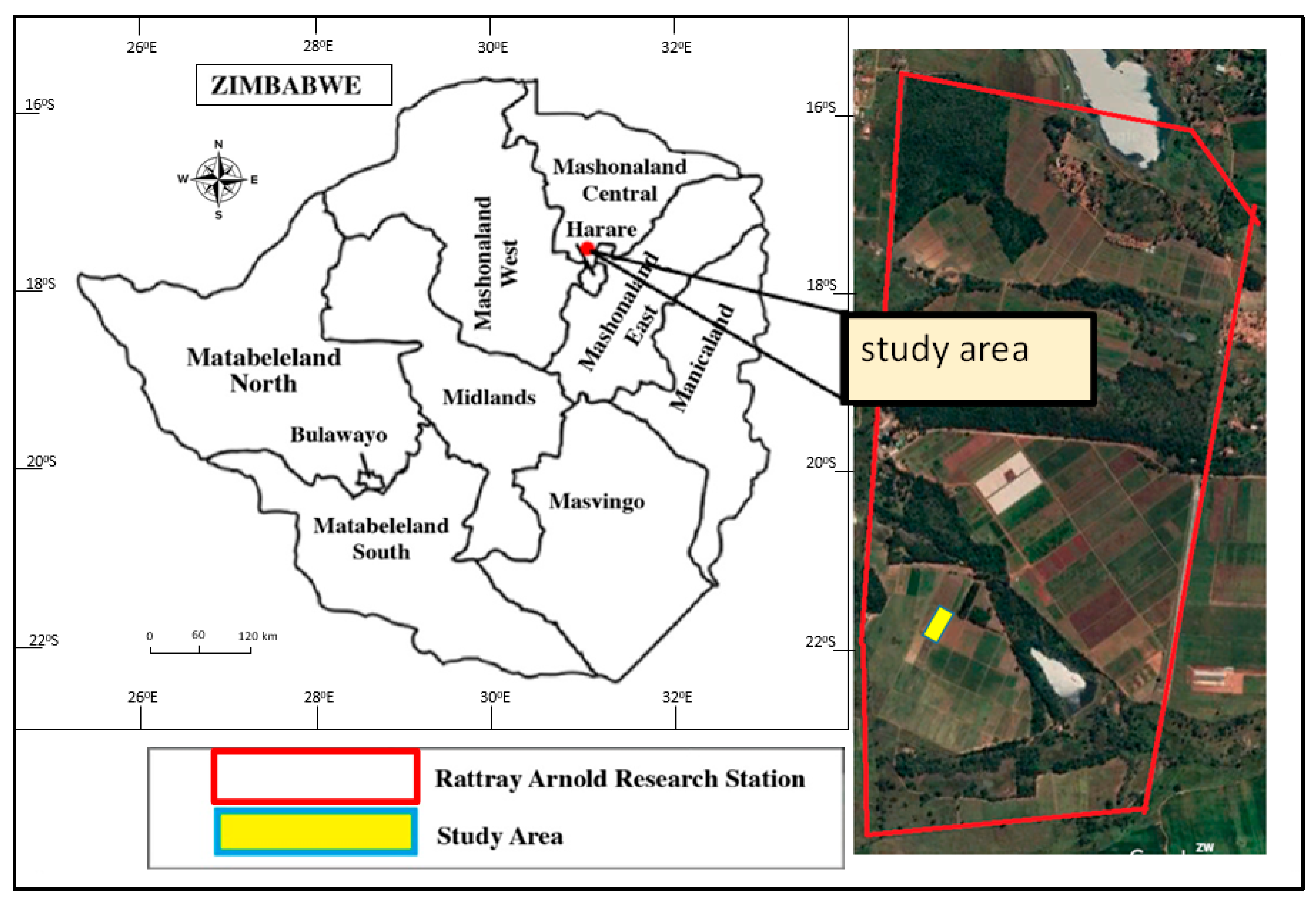
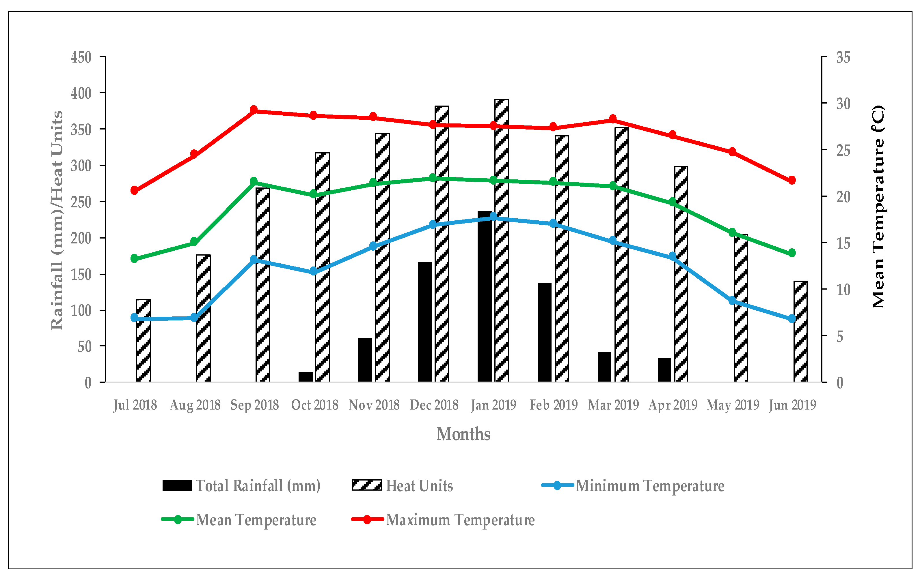
2.1. Study Area

The study was carried out at Rattray Arnold Research Station (RARS) in Zimbabwe, Longitude 31°12′41.35″ E, Latitude 17°40′20.07″ S, and an altitude of 1360 m above sea level (Figure 1). The climate is sub-tropical with a mean temperature range of 28 to 32 °C between November and April, and mean annual precipitation of 865 mm per annum received between November and April. RARS represents the mid-altitude moist environments in Zimbabwe, which is the main maize belt of the country.

The trial was planted on 23 November 2018. The vegetative stage of the crop was in December 2018 and January 2019. Figure 2 shows the monthly rainfall; heat units; and maximum, minimum, and mean temperatures during the crop growing period. The weather data was recorded using an advanced automatic weather station Pro (supplied by Dacom Farm Intelligence, The Netherlands). The weather station Pro was installed outside the experimental plots in the study area to record temperature, relative humidity, rainfall, wind speed, wind direction, and radiation. Plant and insect growth and development depend on temperature, often described as heat units (HU). HU were calculated using Equation (1):

HU = ((Maxi. Temp. + Min. Temp.)/2) − Threshold/Base Temp.

(1)

where HU = heat units and base temperature = 10 °C.

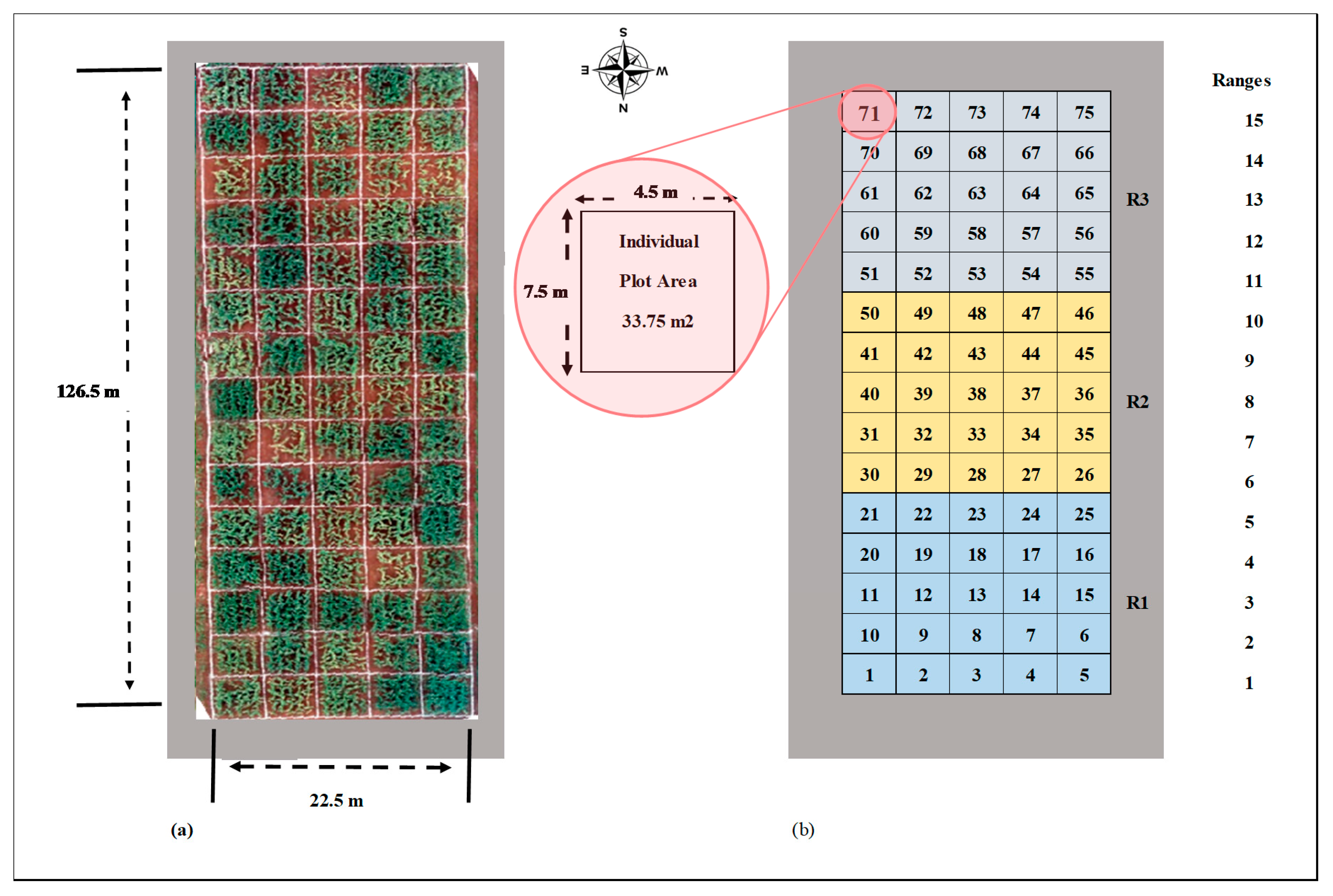
2.2. Maize Varieties, Experimental Design, and Ground Truth Data

Twenty-five maize varieties were grown in a 5 × 5 partially balanced alpha lattice design (Figure 3). A total of 75 six-row plots constituted the experimental area (25 varieties × 3 replications). Three known check varieties representing resistant, moderately resistant, and susceptible responses to MSV were included. Maize seeds were sown on a flat soil surface at 0.5 m within rows and 0.75 m between rows spacing. Four seeds were planted per station and after germination thinned to two at 21 days after sowing to achieve a final plant population of 53,333 plants ha⁻¹. Uniform management was applied to all varieties. Fertilizer application was done at a rate of 450kg ha⁻¹ basal (13:26:13 – N:P:K) at planting. Top dressing was applied at a rate of 450 kg ha⁻¹ using ammonium nitrate (34.5% N) fertilizer. Top dressing was split into two equal amount applications. The first half (225 kg ha⁻¹) of the top dressing was applied at early vegetative and the second half (225 kg ha⁻¹) at booting (pre-flowering) stage. A combination of manual hand weeding and herbicide application was done to keep the experimental plots free of weeds.

To evaluate resistance to MSV, varieties need to be assessed under artificial inoculation where the whole procedure is controlled. Every plant was artificially infested when four leaves had fully expanded with mass reared viruliferous leafhoppers (Cicadulina mbila Naudé) [77] previously fed with MSV infected maize plants.

The white lines on the left image of Figure 3 indicate plot divisions into 75 plots. The individual gross plot area was 7.5 m × 4.5 m × 6 rows, and the whole experimental area was 126.5 m × 22.5 m planted to 25 varieties. The ground truth MSV scores were taken on all 25 maize varieties in all replications. Each plot was rated for MSV using visual scoring at mid-vegetative, flowering, and mid-grain filling growth stages on a scale of 1 to 9. We used the visual scoring of disease severity according to Eyal et al. [78], where 1 denotes resistant (absent to very slight symptoms) and 9 is susceptible (very severe symptoms).

2.3. UAV Platform, Imagery Acquisition, and Processing

2.3.1. The UAV Platform

The imagery was acquired using a Parrot Sequoia multispectral camera mounted on eBee SQ UAV (manufactured by Swiss Geo Consortium Sensefly, Cheseaux-Lausanne, Switzerland). The UAV is a Delta Fixed Wing craft with greater speed and superior aerodynamics compared to multi-rotor craft. It is designed strictly for agricultural purposes. The Parrot sequoia sensor is made up of 5 cameras, with 4 discreet bands: Green (0.53–0.57 μm), Red (0.64–0.68 μm), Rededge (0.73–0.74 μm) and Near-Infrared (0.77–0.81 μm). The fifth camera functions as a composite color capture sensor (red, green, and blue (RGB)). The sensor unit has a sunshine sensor with GPS, sunshine detection unit, and the Inertial Measuring Unit (IMU). The GPS unit receives positional information so that the imagery produced is subsequently georeferenced. The IMU captures the attitudes of the sensor at the times of image capture (through rotations about the X, Y, and Z axes). The sunshine unit captures and records the sunshine radiance value to allow for radiometric correction of the imagery. The imagery was captured using a single grid mapping pattern, with flight plan designed to map an area in excess of the area of interest to minimize the effects of radial distortion around the periphery of the area of interest. The flight plan had the following parameters: 42.5 m altitude, with a ground sampling distance of 8 cm in the RGB and 11.5 cm in the multispectral; 75% forward overlap and 75% side overlap as per Sensefly’s recommendation.

Table 1. UAV sensor parameters and spectral ranges for the Red (R), Green (G), Rededge (RE), and Near-Infrared (NIR) bands of the camera used in this study.

Sensor Specifications	Spectral Features
Sensor type	Multispectral sensor + RGB camera
Multispectral sensor	4-band
RGB resolution	16 mega-pixel (MP), 4608 × 3456 px
Single-band resolution	1.2 MP, 1280 × 960 px
Multispectral bands	Green (0.55 ± 0.04 μm); Red (0.66 ± 0.04 μm); Redeedge (0.735 ± 0.01 μm); Near Infrared (0.79 ± 0.04 μm)
Field of view	64°
Data spectral resolution	Green, Red, Rededge, NIR
Image spatial resolution	11.5 cm at 42.5 m altitude

shows some of the sensor parameters and spectral ranges for the Red (R), Green (G), Rededge (RE), and Near-Infrared (NIR) bands of the camera used.

2.3.2. Image Acquisition and Processing

Aerial imagery was collected at three different phenological stages (mid-vegetative, mid-flowering, and mid-grain filling) using a UAV-mounted multispectral camera. The imagery was processed using Sensefly’s Pix4D Structure from Motion (SfM) software (Cheseaux-Lausanne, Switzerland in collaboration with Pix4D SA, Lausanne, Switzerland). SfM works by finding correspondence between images, features and coordinates by tracking one imagery to the next using the scale-invariant feature transform (SIFT). The SIFT uses the maxima from a difference-of-Gaussians (DOG) pyramid as features. The precise mechanics of Pix4d’s structure from motion are proprietary and therefore cannot be described further. These steps were followed during image processing:

(a)

Initial processing involved key points identification, extraction, and matching; camera model optimization—calibration of the internal (focal length) and external parameters (orientation) of the camera; and geolocation GPS/GCP (Ground Control Points).

(b)

Point cloud and mesh: this step builds on the automatic tie points, which entail point densification and creation of 3D textured mesh.

(c)

Digital Surface Model (DSM) creation to determine orthomosaics and vegetation indices maps. Orthomosaics creation was based on orthorectification to remove perspective distortions from the images to produce vegetation index maps with the value of each pixel with true-to-type reflectance from the area of interest.

Comprehensible mosaics at high spatial resolution (11.5 cm × 11.5 cm) were produced using four multispectral bands: Green (0.53–0.57 μm), Red (0.64–0.68 μm), Rededge (0.73–0.74 μm), and Near-Infrared (0.77–0.81 μm). Spectral reflectance values were extracted and vegetation index (VI) values were calculated per each variety. Maps of VIs were produced at all UAV flight/data acquisition dates (phenological plant stages), showing the evolution of the maize varieties throughout the different phenological stages (Figure 4). The maps are crucial in analyzing the differences between varietal responses to environmental conditions. They provide rich information about the biotic stress that was affecting the varieties. The prevalent biotic stress that was recorded was MSV. The maps generated at the pixel scale allow obtaining precise data to examine the varietal variation for rapid assessment of maize varieties in breeding programs to improve the selection process. Comparison of VIs maps provides excellent visual analysis at different phenological stages (Figure 4).

2.3.3. Reflectance Data Extraction

The imagery captured over the study site was stitched together in Pix4D mapper, which generates two types of multispectral Orthomosaics: the NoAlpha and the transparent mosaics. These were generated for each band of the imagery (Green, Red, Rededge, and NIR). The NoAlpha imagery was used as input into QGIS for reflectance data extraction. A shape file was created by converting a Google earth Key Markup Language (KML) file of the mapped area. The shape file was then used to clip the imagery of the mosaic to the extent of the study area. Shape files were then drawn for each of the compartments (individual plots) according to the experimental layout shown in Figure 3. The “Clip Multiple Layers” plugin was used to simultaneously clip each of the band images using the shapefile for each plot. Once the shapefile compartments were extracted for each shapefile, the maximum, weighted mean, minimum reflectance, and their standard deviations were generated for each plot in each layer. The average reflectance for each plot was determined by taking into account a buffer of 25 cm on each of the four plots sides to restrict the analysis to the center of the plot, making the net plot area 7.0 m × 4.0 m. Ground-truth biophysical measurements for each micro-plot were taken from the center of the plot, consistent with UAV data. Extracted reflectance data were exported into excel spreadsheet format for each of the phenological stages. Vegetation indices were calculated from the plots’ mean reflectance values.

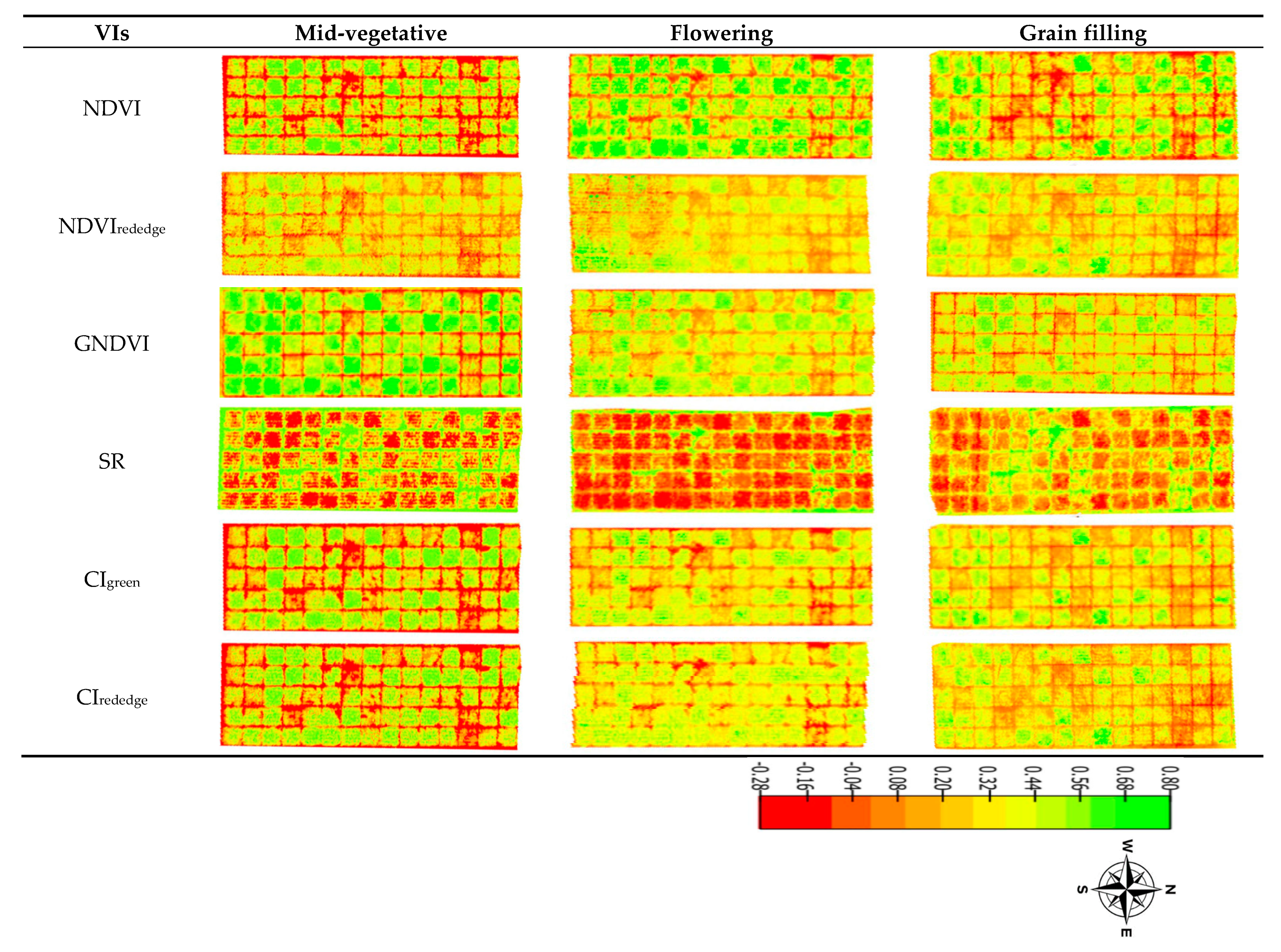
2.3.4. Vegetation Indices

For complete phenotyping, this study used reflectance values in multispectral bands corresponding to Green (0.53–0.57 μm), Red (0.64–0.68 μm), Rededge (0.73–0.74 μm), and Near-Infrared (0.77–0.81 μm) taken at mid-vegetative, flowering, and grain filling stages. The reflectance data were used to calculate the normalized difference vegetation index (NDVI), green normalized difference vegetation index (GNDVI), Rededge NDVI (NDVI_rededge), Simple Ratio (SR), green Chlorophyll Index (CI_green), and Rededge Chlorophyll Index (CI_rededge). Table 2 shows the VIs used in this study.

Table 2. List of vegetation indices (VIs) and their formulas used in this study.

Indices	Equation	Reference
NDVI	$\frac{NIR-Red}{NIR+Red}$	[46]
GNDVI	$\frac{NIR-Green}{NIR+Green}$	[79]
NDVIededge	$\frac{NIR-Rededge}{NIR+Rededge}$	[80]
SR	$\frac{NIR}{Red}$	[81]
CIgreen	$\frac{NIR}{Green}-1$	[82]
CIrededge	$\frac{NIR}{Rededge}-1$	[82]

Table 2. List of vegetation indices (VIs) and their formulas used in this study.

Indices	Equation	Reference
NDVI	$\frac{NIR-Red}{NIR+Red}$	[46]
GNDVI	$\frac{NIR-Green}{NIR+Green}$	[79]
NDVIededge	$\frac{NIR-Rededge}{NIR+Rededge}$	[80]
SR	$\frac{NIR}{Red}$	[81]
CIgreen	$\frac{NIR}{Green}-1$	[82]
CIrededge	$\frac{NIR}{Rededge}-1$	[82]

2.4. Varietal Classification

Prior to varietal classification, we ran descriptive and correlation analyses of ground truth and spectral data. For determining classes, we used the Jenks natural breaks algorithm, which divides a dataset into homogenous classes [83]. One of the requirements of the Jenks method is that the number of desired classes be specified prior to applying the algorithm to the dataset. In this study, the mechanism for determining the classes was based on the fact that for disease evaluation in plant breeding, the main objective is to classify varieties into either resistant or susceptible. However, there are certain varieties that fall in between the two classes. Thus, a third class (moderately resistant) was included and the visual MSV scores were divided into three categories: resistant (1–3.4), moderately resistant (3.5–5.4), and susceptible (5.5–9) for analysis.

The Random Forest model was then used to classify varietal response to MSV under artificial inoculation. RF was chosen for this classification task due to its proven robustness and effectiveness found in other studies for vegetation condition classification in comparison to other supervised parametric and machine learning (ML) classifiers [84,85,86,87]. The RF algorithm also has in-built functionalities for optimizing variables, making it more suitable for classifications that require selection and ranking important variables [87,88]. Furthermore, this study required a robust method suitable for sample sizes that are relatively small and well suited for cross-validation in accuracy assessment [87]. The data were split randomly into training (70%) and validation (30%) sets [89]. The general rule that applies to remote sensing is also important for ML, that one should assess classification accuracy using data not used in training the classifier [90]. Raw data was used for analysis without any correction for experimental design or spatial variability. RF utilizes a specified number of variables (mtry) drawn at each individual node from a random subset of the variables and computes the best split where a subset of variables is used without pruning [91,92,93]. Classification accuracy is improved through RF parameter optimization (mtry and ntree) [91,94]. The RF classification model was developed in this study using the “caret” package within R version 3.6.1 [95].

2.4.1. Variable Optimization

The selection of bands and VIs to use in varietal classification was carried out using the RF variable importance measure. The most important variables were determined and those found important for varietal classification were then used in the model. RF classifier estimates the importance of each input variable to the classification by comparing the magnitude of out-of-bag error when a variable is excluded, while retaining others [96,97]. Thus, RF ranks the variables according to the average error reduction as a result of inclusion of that variable in the classification. Variables with high mean decrease in errors are deemed important for classification and are therefore selected. The tuning of the parameters (ntree and mtry) of RF guarantees high classification accuracy. The default ntree (n = 500) was used. The mtry was optimized by testing all possible values [91,93].

2.4.2. Accuracy Assessment

Confusion matrices were used to assess classification accuracies [98,99]. The overall accuracy (OA) denotes the likelihood that a randomly selected variety is correctly classified according to its reaction to the MSV disease. Ground truth MSV scores were used to assess classification accuracy. The term resistant here was defined as varieties showing no symptoms to very slight symptoms with no effect on final yield; moderately resistant refers to a variety that exhibits symptoms of a partially suppressed virus multiplication and with fewer symptoms than the susceptible. The OA, user’s accuracy (UA), and producer’s accuracy (PA) were determined using the following equations,

$$\mathrm{OA}=\frac{1}{N}{\displaystyle \sum }_{i=1}^r{n}_{ii}\times 100\%$$

(2)

where N is the total number in a confusion matrix, r is the number of rows, and n_ii is the number of varieties correctly classified in a category.

$$\mathrm{PA}=\frac{n_{ii}}{n_{icol}}\times 100\%$$

(3)

$$\mathrm{UA}=\frac{n_{ii}}{n_{irow}}\times 100\%$$

(4)

The Kappa coefficient (Kc), which is also a measure of classification accuracy, was computed as follows [100,101],

$$\mathrm{Kc}=N{\displaystyle \sum }_{n=1}^r\frac{n_{irow}{n}_{icol}}{N^2}-{\displaystyle \sum }_{i=1}^r{n}_{irow}{n}_{icol}$$

(5)

where n_ii is element at position i^th row and i^th column, n_icol is column sums, and n_irow is row sums.

3. Results

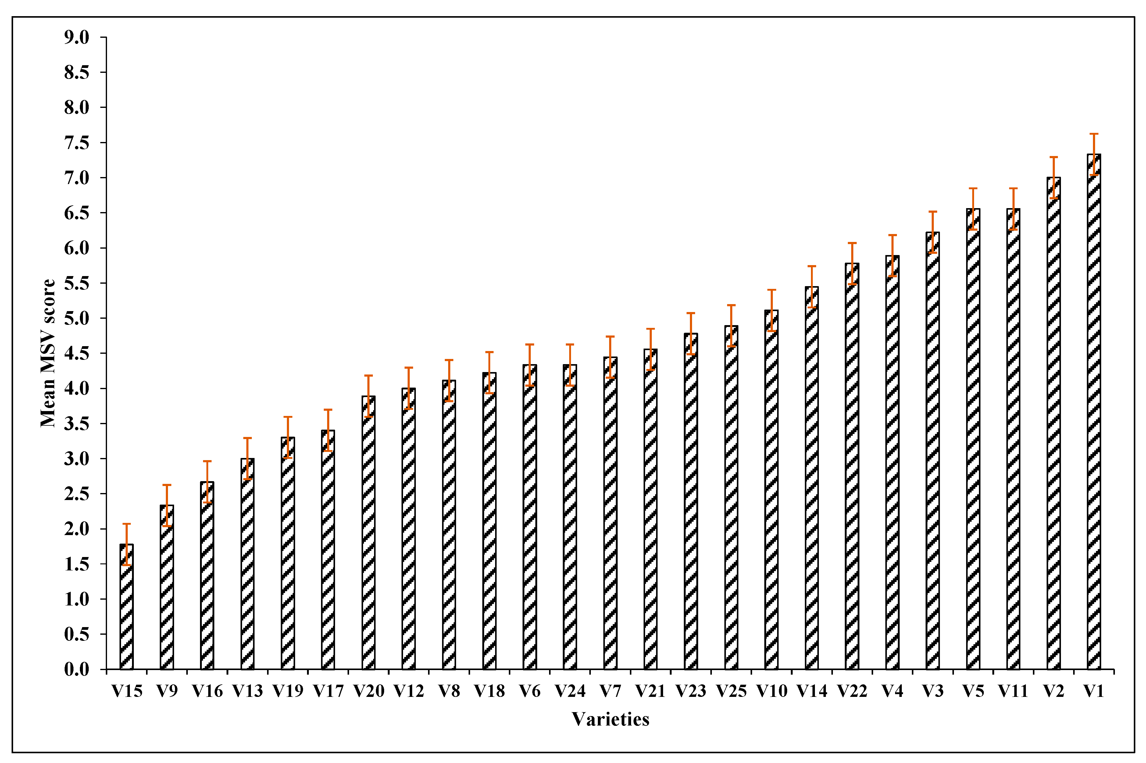
3.1. Varietal Response to MSV

Significant levels of MSV developed on susceptible varieties by their mid vegetative stages. MSV measurements at the different stages were highly correlated (R = 0.88–0.95), thus subsequent models were developed using average MSV severity. Figure 5 represents the mean disease severity scores. Response among varieties differed significantly (p < 0.001) with a maximum severity mean score of up to 7.3 for most susceptible variety on the 1–9 scale. Conversely, the most resistant variety had a mean score of 1.8. Using ground truth data, of the 25 maize varieties tested, six varieties were classified, in order of increasing mean MSV score, as resistant (V15, V9, V16, V13 V19, and V17), twelve as moderately resistant (V20, V12, V8, V18, V6, V24, V7, V21, V23, V25, V10, and V14), and seven varieties as susceptible (V22, V4, V3, V5, V11, V2, and V1) (Figure 5). The best top six varieties in terms of resistant to MSV had mean scores ranging between 1.8 and 3.4.

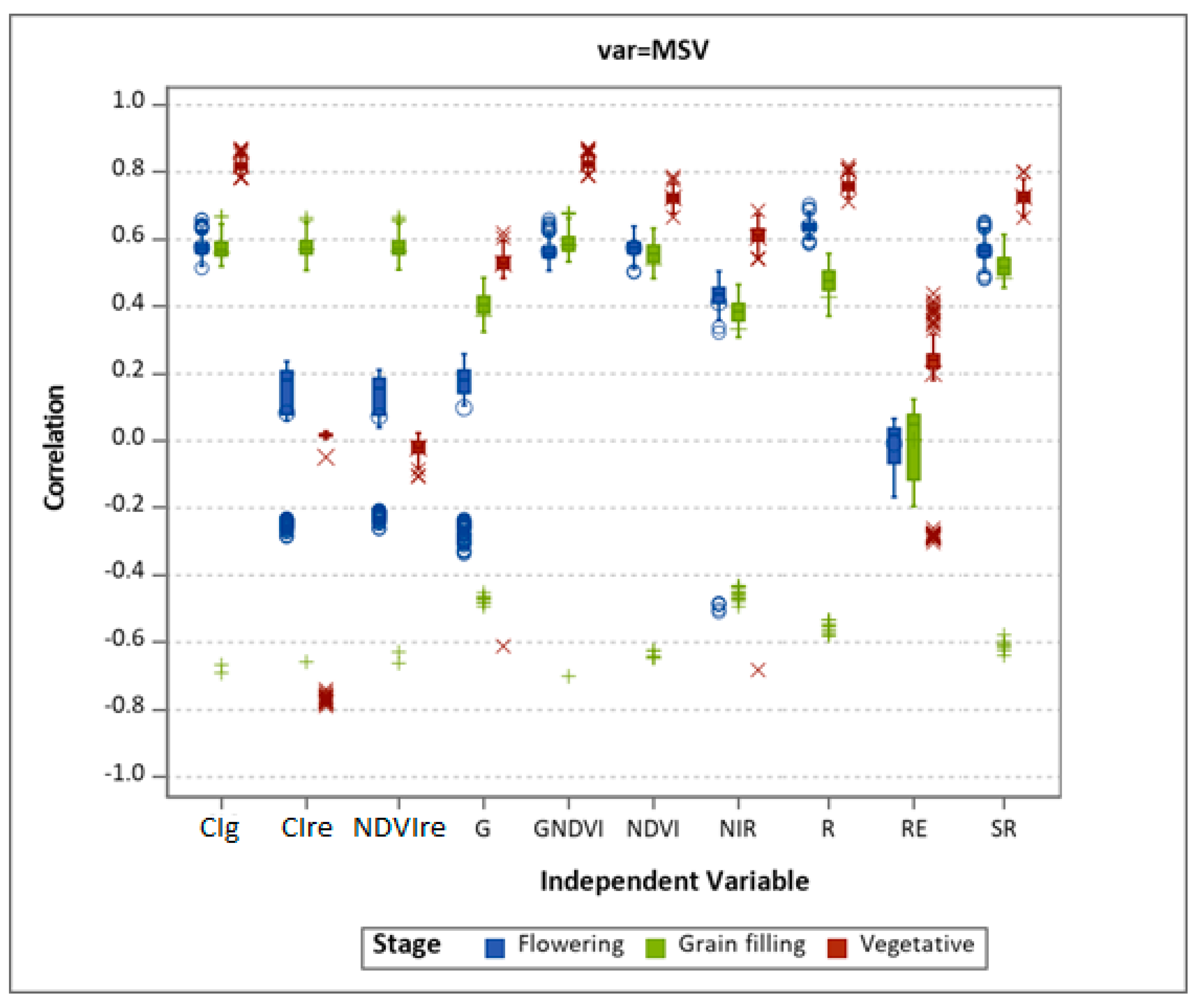
3.2. Comparison of UAV-Derived and Ground Truth Data

A descriptive analysis, including descriptive statistics and correlation of ground truth measurements and UAV-derived data, follows. The analysis shows that there are no outliers in any variable. Figure 6 shows phenotypic correlations between ground-truth (manual) scoring and UAV-derived data at each phenological stage. Correlations between the UAV-derived data and manual MSV scores are significant for the shown variables. In absolute terms, the highest correlations between UAV-derived and manual scoring were Red band (R = 0.78), NDVI (R 0.75), SR (R = 0.74), CI_green (R = 0.83), CI_rededge (R = 0.78), and GNDVI (R = 0.84). These significant agreements between UAV-derived and ground truth data suggest that UAV-based phenotyping of MSV in maize is feasible. This is critical because, to be effective, image-based phenotyping methods need to achieve a level higher or equivalent to the accuracy achieved using manual phenotyping methods, and in a shorter time and at lower costs.

3.3. Phenology-Based Classification Using UAV-Derived Data

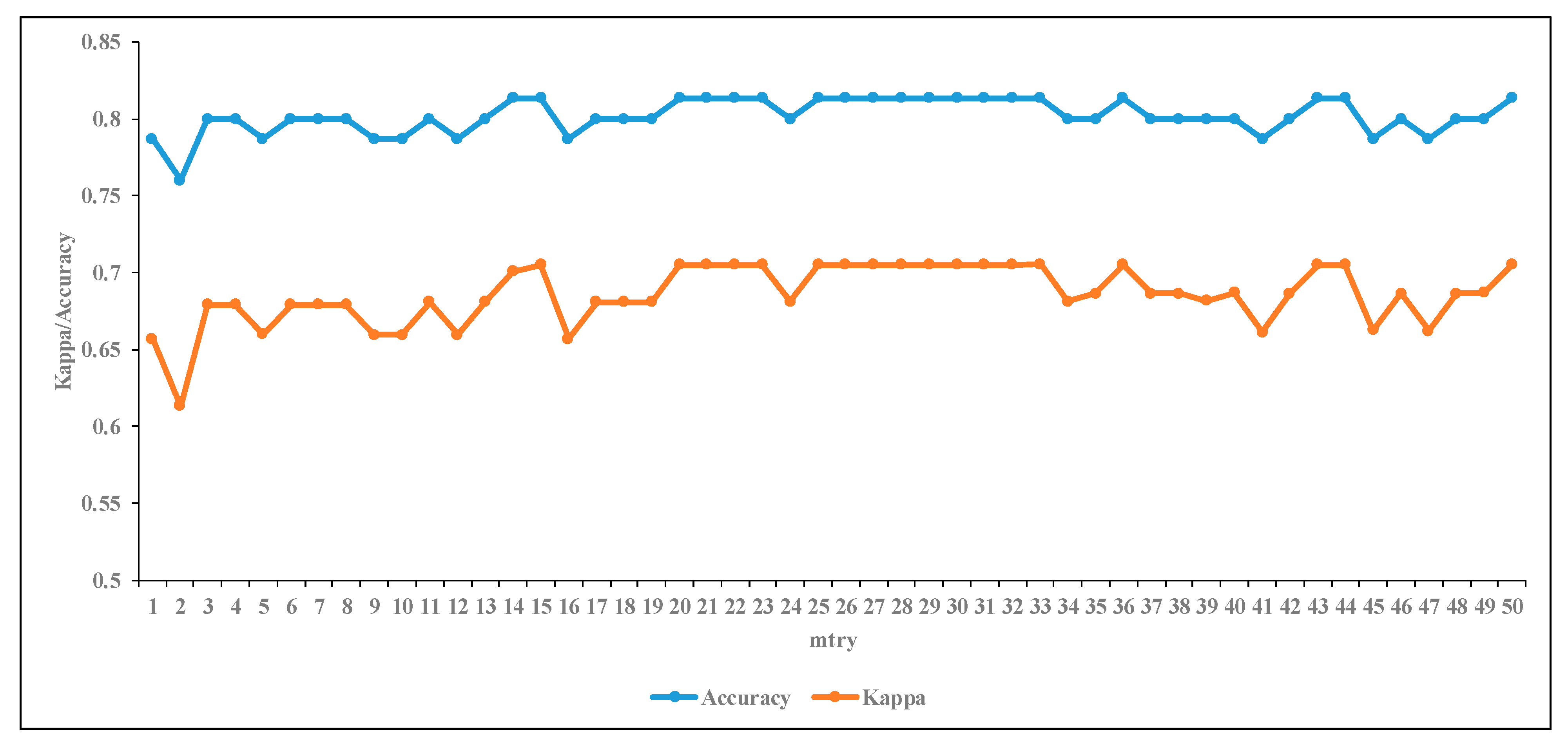
3.3.1. The Effect of RF Input Parameter on Classification

Prior to evaluation of variable importance, we assessed the results of the user-specified parameters (mtry) using the default ntree (n = 500) on the classification accuracy. Figure 7 indicates that the default setting of mtry (n = 14) was the best, beyond which no further improvement in classification accuracy was achieved. The advantage of using the R statistical package is that it provides straightforward optimization techniques, which are not always available in most other commercially available remote sensing software packages [90]. The results showed that when optimizing the RF model, the default setting of mtry is sufficient (in this case mtry = 14) and RF was not sensitivity to the chosen mtry, agreeing with other studies by Liaw and Wiener [102], Díaz-Uriarte and Alvarez de Andrés [103], and Adam et al. [104].

3.3.2. Classification with All Variables

Figure 8 shows all variables used for classification. The different variables were ranked as a measure of their importance in the classification process. The determination of variable importance identified the band(s) and VI(s) that are significant in the classification. An analysis of the four bands at different phenological stages indicates that only Red (vegetative and flowering) and Green (vegetative) bands were ranked in the top ten important variables as significant for classification process using our data. On the other hand, examination of the six VIs shows that five VIs (CI_green, GNDVI, CI_rededge, NDVI, and SR) measured at vegetative stage were selected as important variables for classification of the varieties by the RF model (Figure 8). The overall accuracy of 68.2% (Kc = 0.51) was achieved using all variables. However, to improve the classification accuracy, variable optimization was implemented using RF.

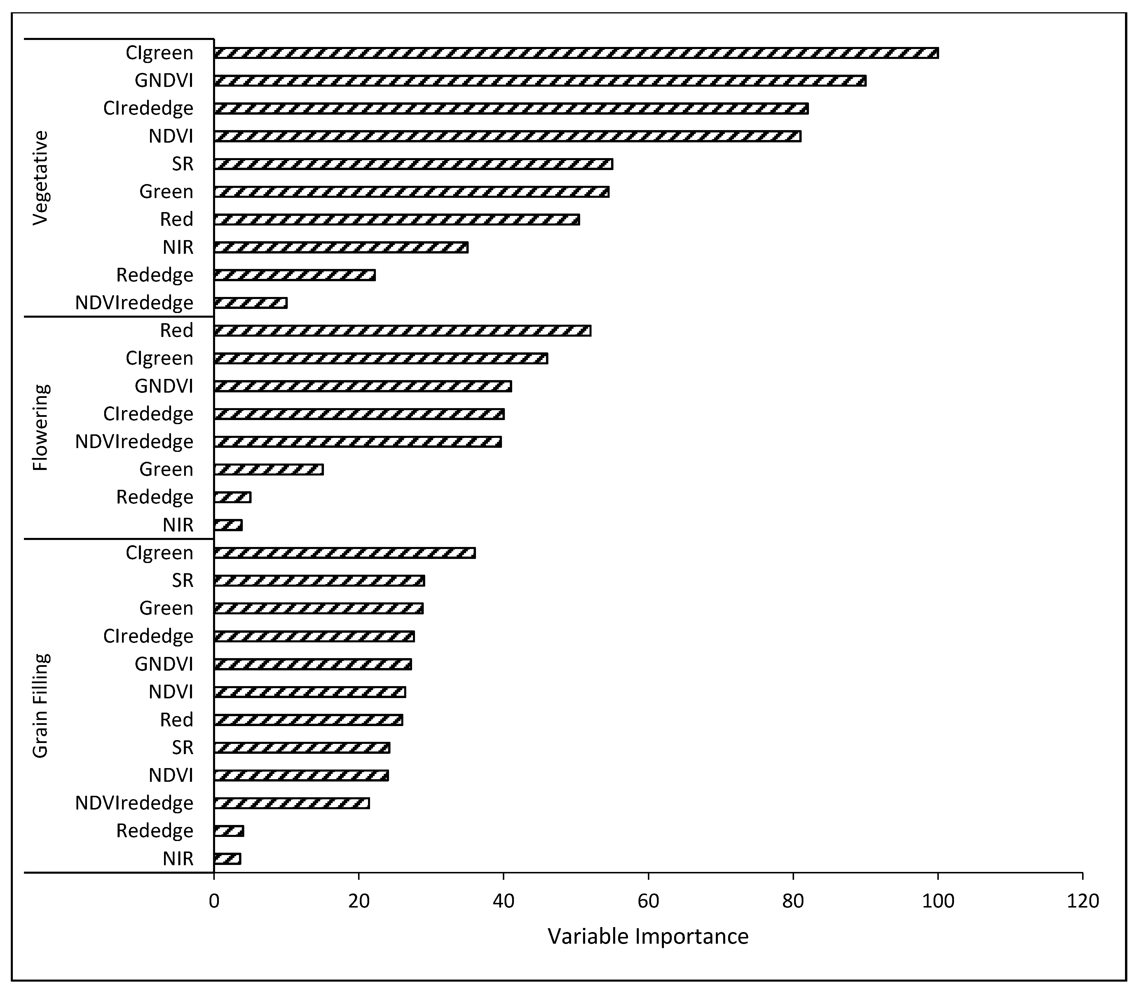
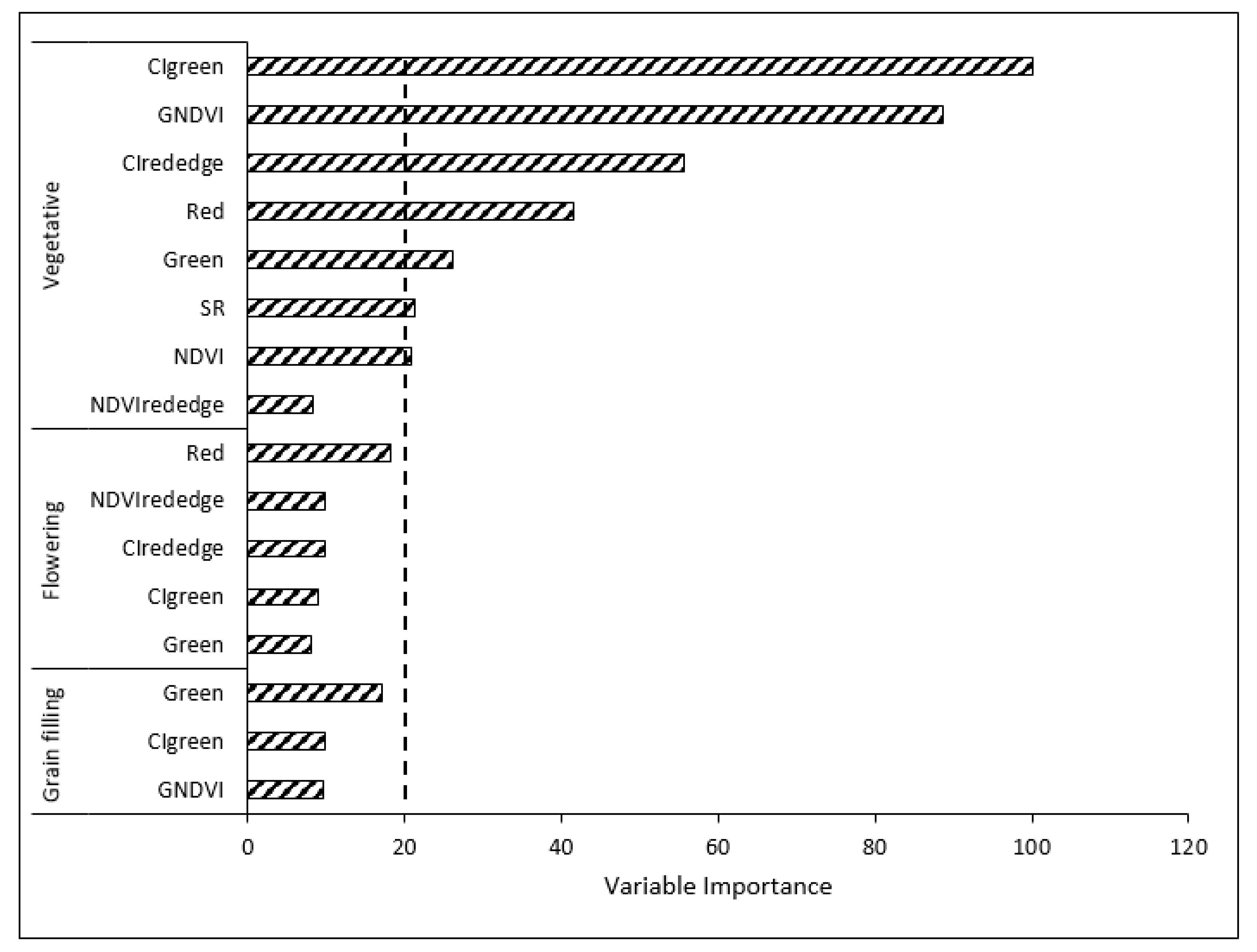
3.3.3. Variable Optimization

Variable optimizing was implemented on all the thirty variables, and only seven variables (i.e., two bands and five VIs) were selected as important using the RF OOB (Figure 9). During optimization the RF model dropped less important variables. Dropping less important variables has been confirmed in others studies to enhance the performance of RF in classification [87,104]. When variable importance is very low, it either means the variable is not important or it is highly collinear with one or more other variables. The two spectral bands (Red and Green) at vegetative stage were retained as important. A total of five VIs (CI_green, GNDVI, CI_rededge, SR, and NDVI) at vegetative stage were selected. All the selected variables by the RF model for classifying different varieties were spectral bands or derived VIs measured at mid-vegetative stage (Figure 9). Therefore, mid-vegetative appeared to be the most appropriate phenological stage for accurate classification of maize varietal response to MSV using UAV-derived multispectral data with RF under artificial MSV inoculation. This might be because after flowering, tassels could mask the detection of MSV by the multispectral cameras.

The variable importance approach used in this article considers each variable individually, assuming all variables are totally independent and not correlated in any way. However, two or more variables may be collinear. One important advantage of RF is that it has functionalities for dealing with collinear variables. To identify if variables are correlated, a correlation matrix was constructed in R at different phenological stages. Highly correlated variables indicates that the variable is completely predictable using the other variables, which means it could be dropped without affecting model accuracy. For example, the CI_green and GNDVI at vegetative stage were highly correlated (R = 0.991). Thus, similar classification results can be achieved using either one of the two. Similarly, SR and NDVI at vegetative stage (R = 0.966), CI_rededge and NDVI_rededge (R = 0.997) at flowering, CI_green and GNDVI (R = 0.997), and SR and NDVI (R = 0.988) at grain filling are highly correlated. The discussion of multicollinearity of these variables is beyond the scope of this article; therefore, the detailed matrix results of multicollinearity are not shown.

3.3.4. Classification Using Optimized Variables

Table 3. Classification accuracies using optimized variables (all seven selected variables were at vegetative stage). PA and UA are producer’s and user’s accuracy, respectively.

	Resistant	Moderately Resistant	Susceptible	Total	UA (%)
Resistant	4	1	0	5	80
Moderately resistant	1	7	1	9	77.8
Susceptible	0	2	6	8	75
Total	5	10	7	22	-
PA (%)	80	70	85.7	-	-
Overall accuracy (%)	77.3	-	-	-	-
Kappa coefficient	0.64	-	-	-	-

shows the results of varietal classification after variable optimization. Use of optimized UAV-derived VIs resulted in increased varietal classification accuracies into different classes (resistant, moderately resistant, and susceptible) compared to variables without optimization. The results indicate a notable improvement in accuracy of varietal classification using optimized variables. The performance of the RF model in classifying the varieties was improved through variable optimization, with the RF model achieving overall varietal classification accuracies of 77.3% (Kc = 0.64) with optimized variables compared to 68.2% (Kc = 0.51) without variable optimization, representing an improvement of ~13.3%. Furthermore, optimization reduced the number of variables from thirty to seven, which were then used by the RF model (Figure 9). Improvement in classification accuracies obtained in this study agrees with previous work by Adam et al. [104] and Chemura et al. [87], who found improvements in classification accuracies when variables are optimized. Moreover, our results are comparable to the accuracies found by Sankaran et al. [105] using ground-based sensors.

4. Discussion

The recent progresses in the use of sensing and imaging systems, including UAV-derived data with high spatial (submeter) and temporal (daily/weekly) resolution, present a step-change towards data availability and turnaround time in varietal analysis for quick and robust high-throughput plant phenotyping in plant breeding programs. This study set out to assess the utility of UAV-derived multispectral data for improved phenotyping of maize varietal response to MSV disease under field conditions. The UAV-derived VIs maps produced using UAV-derived data show comprehensive temporal and spatial variations at varietal level (Figure 4), providing significant information about the variability in varietal response that can be explained by varietal interaction with the MSV disease. Although UAV-derived multispectral imageries have limited spectral range and resolution, they offer robust spatial and temporal resolutions that allow variation associated with different varieties to be quantified. Maize varieties are evaluated for disease resistance to select appropriate varieties for the target production environment, to address global food demand and responding to changing climate conditions. Undoubtedly, the continuing climate changes are threatening the currently vulnerable global food security in a number of ways, as well as exacerbating major crop diseases and creating weather conditions conducive for the emergence of new devastating diseases in major food-producing regions. Therefore, the call for intensified crop breeding efforts and the need to bring phenotyping up to speed with genomics by harnessing the power of computing, robotics, machine learning (ML), artificial intelligence, and image analysis is urgent, if we hope to meet the global food demand to feed 10 billion people by 2050.

4.1. Comparison of UAV-Derived Data and Ground Truth Measurements

There were generally strong correlations between UAV-derived data and ground-based MSV scoring in this study, suggesting the value of UAV-derived data in plant phenotyping. These are encouraging results given the bottlenecks experienced in manual phenotyping, especially in plant breeding where screening of a large number of varieties is needed before suitable ones are selected for advancement, release, and commercialization. Our results agree with Garcia-Ruiz et al. (64) who found significant correlation between UAV-based data and the ground truth measurements for detection of bacterial Huanglongbing (Citrus Greening) disease in citrus trees. Jarolmasjed et al. [106] compared UAV-derived multispectral imaging data and found significant correlation with ground truth rating of fire blight disease (Erwinia amylovora) in apples. Similarly, Mahlein et al. [107] also reported a significant agreement (R² = 0.89) between NDVI and ground truth leaf disease severity with a classification accuracy of 80% in sugarbeet Cercospora leaf spot. Jansen et al. [108], using noninvasive spectral phenotyping to screen Cercospora disease resistance in sugar beet, similarly established significant correlations between spectral data and ground truth scores confirming the potential use of remotely sensed data in disease resistance phenotyping.

However, most of these studies were based on snapshot (single phenological stage) spectral data collection. Our approach in this study was based on multitemporal spectral data. For example, Garcia-Ruiz et al. [64] recommended that future work should study temporal effects in aerial remote sensing of plant diseases. Thus, using multitemporal data, we identified not only the optimal bands and indices, but also the ideal growth stage for accurate varietal phenotyping. The results demonstrated that VIs measured at vegetative stage are the most important for classification of maize varietal response to MSV. The MSV disease symptoms on a susceptible variety result in changes in color, size and shape. Our results show that these morpho-physical changes can be measured accurately using spectral data at the vegetative stage. Furthermore, measurements after flowering could suffer from masking effects by the flowers (tassels) and old senescing leaves at mid-grain filling.

4.2. RF Classification Performance Using Spectral Bands and VIs

The results of this study show that UAV-derived VIs produced plausible varietal classification and that the majority of selected important variables were VIs compared to spectral bands (Figure 9). This agrees with previous studies, for example, Chemura et al. [87] who found vegetation indices to perform better than spectral bands in discriminating coffee (Coffea arabica) leaf rust (Hemileia vastatrix) using RF. Furthermore, the overall classification accuracy results obtained in this study using UAV-derived multispectral VIs are comparable to similar studies. For example, Garcia-Ruiz et al. [64], using UAV-based multispectral data from six bands and seven indices for classification and identification of citrus greening disease, obtained accuracies ranging from 62% to 82% using linear discriminant analysis and between 63% and 85% using support vector machines. As indicated above, our study demonstrates that crop phenological stage is critical when assessing varietal variation in crop phenotyping using UAV remotely sensed data. Most of the best selected variables were measured at the vegetative stage (Figure 9). This is important in field-based high-throughput plant phenotyping for characterizing maize varieties at multiple scales, and at different levels of resolution and dimensionality using remote sensing. Thus, aerial imaging using UAVs can offer the plant breeding, phenotyping, and remote sensing community the ability to quickly record high temporal and spatial resolution data for maize varietal analysis and allow rapid, cost-effective, and comprehensive data-driven variety selection and release in plant breeding programs. Robust plant phenotyping is critical in plant breeding because it forms the basis for selection of new varieties. However, UAVs do not provide a substitute for the breeder’s eye, but augment the effort and inform better phenotype-based selections [24]. The advantage of the UAV-based imaging data is the high-throughput capability and ability to measure multiple traits instantaneously [109,110]. Furthermore, UAV-based phenotyping does not suffer from low repeatability associated with manual records [111]. Thus, UAVs eliminate subjectivity and reduce labor costs, spatial singularity, and fatigue associated with manual methods [87,112]. Additionally, the naked eye may not be able to identify physiological/metabolic differences caused by different stresses [113], which can be possible with imaging tools [114]. For example, Nutter et al. [115] found improved precision in characterizing bent grass dollar spot (Agrostis palustris Huds.) using spectral data compared to a visual scoring method. Condorelli et al. [111] reported higher repeatability when screening drought-adaptive traits in wheat using UAV phenotyping methods compared to ground-based methods.

4.3. Variable Optimization Effect on RF Algorithm Classification

In this study, RF successfully ranked each variable importance both UAV bands and VIs on the classification output (Figure 8 and Figure 9), providing an insight into which UAV-derived bands and VIs are critical in the classification process using our data. The classification improved by ~13.3%, when optimized variables were used indicating that variable importance is efficient and improves RF modeling. There are various reasons why variable optimization achieves better classification results in comparison to using all available variables. For example, Chemura et al. [87] reasoned that multispectral sensors are meant for multiple purposes that range from water, agricultural, forestry to urban applications, and therefore just a limited number of parameters may be useful for the intended purpose. Furthermore, several variables maybe correlated or may not provide useful information, and these are dropped in the classification and modeling process. The removal of these redundant variables enables the model to achieve better results, agreeing with studies by Pal and Foody [116] and Chemura et al. [87].

Machine learning algorithm classification accuracy is affected by training data quality, sample size, and user-specified parameters [117]. In this study, the sample size was relatively small (n = 75), split randomly into training (70%) and validation (30%), and a robust RF model suitable for such scenarios was used, consistent with the recommendation by Maxwell et al. [90]. In parametric maximum likelihood classifiers, the rule of thumb requires the training sample be at least 10 times the number of variables [118]. However, for ML classifiers, the literature is silent on the optimum size of the training sample [90]. Huang et al. [117] posit that in ML, the size of the training sample may vary depending on the ML algorithm used and the number of input variables. On the other hand, Lu and Weng [119] and Li et al. [120] recommended a large training data set regardless of the algorithm used. Indeed, Huang et al. [117] showed that increased training sample size gave higher accuracy. However, in practice, there is a need to balance the size, quality, cost, and the limited time available. RF has been found to be insensitive to the size of training sample compared to single decision trees methods [121,122], and has proved to be appropriate for small samples in disease classification in coffee leaf rust [87], in Sirex noctilio infestation in pine trees [123], and classification of alfalfa (14 training samples) and oats (with only five training samples) [90].

4.4. The Utility of UAV-Based Multispectral Data in High-Throughput Phenotyping

Most of the recent studies that systematically attempt to validate spectral indices in plant phenotyping at field scale are based on proximal measurements [45,49,87]. However, proximal sensing is associated with the challenges alluded to above. It is difficult to use when fields are under irrigation or pesticides applications, and not practical for rapid evaluation of multiple varieties at scale and high temporal resolution in breeding programs [20,50]. Furthermore, proximal remotely sensed data can fail a precision test for high-throughput because of fluctuations in weather conditions in between measurements (i.e., from start to finish), which may take one to several hours where large numbers of breeding plots are involved [49]. Extended time taken in manual scoring introduces variation due to phenological changes, environmental conditions, and recorder fatigue thereby affecting repeatability and leading to inaccurate data and even unjustified conclusions [111,124]. Speed is therefore essential in achieving high precision in high-throughput phenotyping. Although this study did not compare the time difference between manual scoring and UAV-based phenotyping, researchers have found UAV-based phenotyping to be 10 times faster than manual scoring [125]. Similarly, Guan and Nutter [126] found remote sensing to be 15 times faster at estimating alfalfa leaf disease. Therefore, UAV offers real-time and fast crop phenotyping and will reduce dependence on time-consuming and resource-intensive manual phenotyping in plant breeding and varietal evaluation, leading to speeding up breeding and selection processes.

The opportunities presented by UAV-derived data have to take into account the practical limitations imposed by field conditions to the applications of the technology where a complex of different diseases are existing in the same field or area of interest. The UAV-derived spectral bands and indices applied in this study are not disease-specific (to the best of our knowledge), and therefore can only be useful in quantifying different levels of infestation or damage when a single disease affects the crop with no ability to distinguish between different types of diseases. This makes the current UAV-derived spectral data relevant in phenotyping of disease with a prior knowledge of the type of disease that exists in the target area of interest. Studies into development of disease-specific VIs have been reported [107,127,128]. However, this is an area that needs further exploration. In addition, although VIs derived from multispectral data are informative, they utilize less than 1% of available spectra [129], and as such may lack detail compared to, for example, hyperspectral data. Therefore, further investigations are necessary to refine the use of UAV-derived data in high-throughput crop phenotyping. It is also noteworthy to mention that this study only used one ML algorithm (RF), while there are several other classifiers, which can be used.

4.5. Leveraging High-Throughput Image-Based Phenotyping Technology to Fast-Track Crop Improvement under Changing Climate Conditions

MSV disease can be controlled using systemic insecticides that control the vector through spraying or treatment of seed. However, spraying and use of seed treatments against MSV are expensive and beyond the reach of most of the resource-poor farmers. Furthermore, spraying and seed treatment options offer only temporary protection when disease pressure is severe. The development and cultivation of varieties tolerant or resistant to MSV is arguably the most cost-effective and climate-smart way of preventing MSV epidemics and protecting farmers’ livelihoods. To breed for resistance, breeders evaluate large numbers of lines or varieties to select suitable ones for commercialization. However, as previously alluded to, rapid and accurate phenotyping of traits associated with grain yield is presently creating serious bottlenecks [20,28]. Robust phenotyping is critical in plant breeding programs because it forms the basis for new variety selection. In this study, our method has demonstrated the utility of image-based high-throughput phenotyping to relieve the breeding community of phenotyping bottlenecks. Image-based high-throughput phenotyping technology will help accelerate crop breeding in the face of changing climate conditions and associated new challenges. This will be achieved by screening large numbers of varieties for multiple traits with higher accuracy and at reduced costs [35]. In addition, high-throughput image-based phenotyping will enable the evaluation of physiological/metabolic differences caused by different stresses [113], which may not be possible with the naked eye but possible with imaging tools [114,130]. This will help broaden the genetic variation in the germplasm pool if such traits are accumulated in the breeding pipeline. Furthermore, high-throughput phenotyping data can be combined with genomic data to further improve genetic gain [130,131,132]. The key to the successful application of image-based high-throughput plant phenotyping for diseases and other stresses lies in our ability to develop reproducible protocols that are user-friendly, including image-based data retrieval, analysis, and interpretation. This will increase crop genetic improvement efficiency and our ability to satisfy future food requirements, especially as climate change accelerates.

5. Conclusions

This study evaluated the utility of UAV-derived multispectral data with the RF algorithm to classify different maize varieties under artificial MSV inoculation. The results showed that UAV-based multispectral data combined with advanced classifier RF analysis can be useful in field-based high-throughput maize phenotyping. Therefore, we conclude the following.

• UAV-based remotely sensed data provides plausible accuracy, thereby offering a step-change towards data availability and turnaround time in varietal analysis for quick and robust high-throughput plant phenotyping in maize breeding and variety evaluation programs, to address the vagaries brought by climate change and meet global food security. Specifically, the study has demonstrated that VIs measured at vegetative stage are the most important for classification of maize varieties under artificial MSV inoculation using UAVs.
• UAV-derived remotely sensed data correlates well with ground truth measurements, confirming the utility of a UAV approach in field-based high-throughput phenotyping in breeding programs, where final varietal selection must be based on extensive screening of multiple genotypes. This will reduce selection bottlenecks caused by manual phenotyping and offers decision support tools for large-scale varietal screening.
• Variable optimization improves classification accuracy when compared to the use of variables without optimization. Thus, the RF classifier is a robust algorithm capable of determining the depth of variable importance and their rankings using our data.
• Image-based high-throughput phenotyping can relieve the breeding community of phenotyping bottlenecks usually experienced when evaluating large populations of genotypes in order to accelerate crop breeding and selection addressing multiple stresses associated with climate change.

The study shows that cost-effective UAV-derived multispectral data is capable of classifying maize varieties susceptible to MSV with good accuracy, and therefore can complement and eventually replace visual ratings, especially for large-scale canopy-level measurements when multiple genotypes are evaluated in plant breeding. However, current VIs are not disease-specific and therefore can only be useful in different levels of infestation or damage due to a singly present disease with no ability to distinguish between complex types of diseases. This makes the current UAV-derived spectral data relevant in phenotyping of disease with a prior knowledge of the type of disease that exists in the target area of interest. Three research gaps have been identified for further inquiry: (i) comparison of multiple ML algorithms to identify the best performing classier(s); (ii) evaluation of whether UAVs mounted with hyperspectral high-resolution cameras improve detection and classification accuracies; and (iii) development of disease-specific VIs.

References

1. Alston, J.M.; Beddow, J.M.; Pardey, P.G. Agricultural Research, Productivity, and Food Prices in the Long Run. Science 2009, 325, 1209–1210. [Google Scholar] [CrossRef] [PubMed]
2. Godfray, H.C.J.; Beddington, J.R.; Crute, I.R.; Haddad, L.; Lawrence, D.; Muir, J.F.; Pretty, J.; Robinson, S.; Thomas, S.M.; Toulmin, C. Food Security: The Challenge of Feeding 9 Billion People. Science 2010, 327, 812–818. [Google Scholar] [CrossRef] [PubMed] [Green Version]
3. Intergovernmental Panel on Climate Change. Climate change: Synthesis report. In Contribution of Working Groups I, II and III to the Fifth Assessment Report of the Intergovernmental Panel on Climate Change; Pachauri, R.K., Meyer, L.A., Eds.; IPCC: Geneva, Switzerland, 2014. [Google Scholar]
4. Velásquez, A.C.; Castroverde, C.D.M.; He, S.Y. Plant-Pathogen Warfare under Changing Climate Conditions. Curr. Boil. 2018, 28, R619–R634. [Google Scholar] [CrossRef] [PubMed]
5. Coakley, S.M.; Scherm, H.; Chakraborty, S. Climate Change and Plant Disease Management. Annu. Rev. Phytopathol. 1999, 37, 399–426. [Google Scholar] [CrossRef]
6. Garrett, K.A.; Dendy, S.P.; Frank, E.E.; Rouse, M.N.; Travers, S.E. Climate Change Effects on Plant Disease: Genomes to Ecosystems. Annu. Rev. Phytopathol. 2006, 44, 489–509. [Google Scholar] [CrossRef] [Green Version]
7. Luo, Y. The Effects of Global Temperature Change on Rice Leaf Blast Epidemics: A Simulation Study in Three Agroecological Zones. Agric. Ecosyst. Environ. 1998, 68, 187–196. [Google Scholar] [CrossRef]
8. Garrett, K.A.; Forbes, G.; Savary, S.; Skelsey, P.; Sparks, A.H.; Valdivia, C.; Van Bruggen, A.H.C.; Willocquet, L.; Djurle, A.; Duveiller, E.; et al. Complexity in climate-change impacts: An analytical framework for effects mediated by plant disease. Plant Pathol. 2011, 60, 15–30. [Google Scholar] [CrossRef] [Green Version]
9. Rose, D.J.W. Epidemiology of Maize Streak Disease. Annu. Rev. Èntomol. 1978, 23, 259–282. [Google Scholar] [CrossRef]
10. IPCC. Fourth Assessment Report: Synthesis. 2007. Available online: http://www.ipcc.ch/pdf/assessment-report/ar4/syr/ar4_syr.pdf (accessed on 28 July 2020).
11. Kloppers, F. Maize Diseases: Reflection on the 2004/2005 Season. 2005. Available online: http://saspp.org/index2.php?option=com_content&do_pdf=1&id=2 (accessed on 28 July 2020).
12. Stanley, J.; Boulton, M.I.; Davies, J.W. Geminiviridae. In Embryonic Encyclopedia of Life Sciences; Nature Publishing Group: London, UK, 1999. [Google Scholar]
13. Efron, Y.; Kim, S.K.; Fajemisin, J.M.; Mareck, J.H.; Tang, C.Y.; Dabrowski, Z.T.; Rossel, H.W.; Thottappilly, G.; Buddenhagen, I.W. Breeding for Resistance to Maize Streak Virus: A Multidisciplinary Team Approach1. Plant Breed. 1989, 103, 1–36. [Google Scholar] [CrossRef]
14. Rossel, H.W.; Thottappilly, G. Virus Diseases of Important Food Crops in Tropical Africa; International Institute of Tropical Agriculture (IITA): Ibadan, Nigeria, 1985; p. 61. [Google Scholar]
15. Njuguna, J.A.M.; Kendera, J.G.; Muriithi, L.M.M.; Songa, S.; Othiambo, R.B. Overview of maize diseases in Kenya. In Maize Review Workshop in Kenya; Kenya Agricultural Research Institute: Nairobi, Kenya, 1990; pp. 52–62. [Google Scholar]
16. Dabrowski, Z.T. Cicadulina Ghaurii (Hem., Euscelidae): Distribution, Biology and Maize Streak Virus (MSV) Transmission. J. Appl. Entomol. 1987, 103, 489–496. [Google Scholar] [CrossRef]
17. Phillips, R.L. Mobilizing Science to Break Yield Barriers. Crop. Sci. 2010, 50, S99–S108. [Google Scholar] [CrossRef] [Green Version]
18. Poland, J. Breeding-Assisted Genomics. Curr. Opin. Plant Boil. 2015, 24, 119–124. [Google Scholar] [CrossRef] [PubMed]
19. Bilder, R.M.; Sabb, F.W.; Cannon, T.D.; London, E.D.; Jentsch, J.D.; Parker, D.S.; Poldrack, R.A.; Evans, C.; Freimer, N.B. Phenomics: The Systematic Study of Phenotypes on a Genome-Wide Scale. Neuroscience 2009, 164, 30–42. [Google Scholar] [CrossRef] [PubMed] [Green Version]
20. Araus, J.L.; Cairns, J.E. Field High-Throughput Phenotyping: The New Crop Breeding Frontier. Trends Plant Sci. 2014, 19, 52–61. [Google Scholar] [CrossRef] [PubMed]
21. Ghanem, M.E.; Marrou, H.; Sinclair, T.R. Physiological Phenotyping of Plants for Crop Improvement. Trends Plant Sci. 2015, 20, 139–144. [Google Scholar] [CrossRef] [PubMed]
22. Sankaran, S.; Khot, L.R.; Espinoza, C.Z.; Jarolmasjed, S.; Sathuvalli, V.; VanDeMark, G.J.; Miklas, P.N.; Carter, A.H.; Pumphrey, M.; Knowles, N.R.; et al. Low-Altitude, High-Resolution Aerial Imaging Systems for Row and Field Crop Phenotyping: A Review. Eur. J. Agron. 2015, 70, 112–123. [Google Scholar] [CrossRef]
23. Tardieu, F.; Cabrera-Bosquet, L.; Pridmore, T.; Bennett, M.J. Plant Phenomics, from Sensors to Knowledge. Curr. Boil. 2017, 27, R770–R783. [Google Scholar] [CrossRef]
24. Hickey, L.; Hafeez, A.N.; Robinson, H.M.; Jackson, S.A.; Leal-Bertioli, S.C.M.; Tester, M.; Gao, C.; Godwin, I.D.; Hayes, B.J.; Wulff, B.B.H. Breeding Crops to Feed 10 Billion. Nat. Biotechnol. 2019, 37, 744–754. [Google Scholar] [CrossRef] [Green Version]
25. Fahlgren, N.; Gehan, M.A.; Baxter, I. Lights, Camera, Action: High-Throughput Plant Phenotyping Is Ready for a Close-Up. Curr. Opin. Plant Boil. 2015, 24, 93–99. [Google Scholar] [CrossRef] [Green Version]
26. White, J.; Andrade-Sanchez, P.; Gore, M.A.; Bronson, K.F.; Coffelt, T.A.; Conley, M.M.; Feldmann, K.A.; French, A.; Heun, J.T.; Hunsaker, D.; et al. Field-Based Phenomics for Plant Genetics Research. Field Crop. Res. 2012, 133, 101–112. [Google Scholar] [CrossRef]
27. Zaman-Allah, M.; Vergara, O.; Araus, J.L.; Tarekegne, A.; Magorokosho, C.; Zarco-Tejada, P.J.; Hornero, A.; Albà, A.H.; Das, B.; Craufurd, P.Q.; et al. Unmanned Aerial Platform-Based Multi-Spectral Imaging for Field Phenotyping of Maize. Plant Methods 2015, 11, 1–10. [Google Scholar] [CrossRef] [PubMed] [Green Version]
28. Furbank, R.T.; Tester, M. Phenomics—Technologies to Relieve the Phenotyping Bottleneck. Trends Plant Sci. 2011, 16, 635–644. [Google Scholar] [CrossRef] [PubMed]
29. Cobb, J.N.; Declerck, G.; Greenberg, A.J.; Clark, R.; McCouch, S.R.M. Next-Generation Phenotyping: Requirements and Strategies for Enhancing Our Understanding of Genotype-Phenotype Relationships and Its Relevance to Crop Improvement. Theor. Appl. Genet. 2013, 126, 867–887. [Google Scholar] [CrossRef] [Green Version]
30. Dhondt, S.; Wuyts, N.; Inzé, D. Cell to Whole-Plant Phenotyping: The Best Is Yet to Come. Trends Plant Sci. 2013, 18, 428–439. [Google Scholar] [CrossRef] [PubMed]
31. Fiorani, F.; Schurr, U. Future Scenarios for Plant Phenotyping. Annu. Rev. Plant Boil. 2013, 64, 267–291. [Google Scholar] [CrossRef] [PubMed] [Green Version]
32. Anthony, D.; Detweiler, C. UAV Localization in Row Crops. J. Field Robot. 2017, 34, 1275–1296. [Google Scholar] [CrossRef]
33. Deery, D.M.; Jimenez-Berni, J.A.; Jones, H.G.; Sirault, X.R.R.; Furbank, R.T. Proximal Remote Sensing Buggies and Potential Applications for Field-Based Phenotyping. Agronomy 2014, 4, 349–379. [Google Scholar] [CrossRef] [Green Version]
34. Prashar, A.; Jones, H.G. Infra-Red Thermography as a High-Throughput Tool for Field Phenotyping. Agronomy 2014, 4, 397–417. [Google Scholar] [CrossRef]
35. Mahlein, A.-K. Plant Disease Detection by Imaging Sensors—Parallels and Specific Demands for Precision Agriculture and Plant Phenotyping. Plant Dis. 2016, 100, 241–251. [Google Scholar] [CrossRef] [Green Version]
36. Báez-González, A.D.; Chen, P.-Y.; Tiscareño-López, M.; Srinivasan, R. Using Satellite and Field Data with Crop Growth Modeling to Monitor and Estimate Corn Yield in Mexico. Crop. Sci. 2002, 42, 1943–1949. [Google Scholar] [CrossRef]
37. Battude, M.; Al Bitar, A.; Morin, D.; Cros, J.; Huc, M.; Sicre, C.M.; Le Dantec, V.; Demarez, V. Estimating Maize Biomass and Yield Over Large Areas Using High Spatial and Temporal Resolution Sentinel-2 Like Remote Sensing Data. Remote Sens. Environ. 2016, 184, 668–681. [Google Scholar] [CrossRef]
38. Hoffer, N.V.; Coopmans, C.; Jensen, A.M.; Chen, Y.Q. A Survey and Categorization of Small Low-Cost Unmanned Aerial Vehicle System Identification. J. Intell. Robot. Syst. 2013, 74, 129–145. [Google Scholar] [CrossRef]
39. Jimenez-Berni, J.A.; Zarco-Tejada, P.J.; Suarez, L.; Fereres, E. Thermal and Narrowband Multispectral Remote Sensing for Vegetation Monitoring From an Unmanned Aerial Vehicle. IEEE Trans. Geosci. Remote Sens. 2009, 47, 722–738. [Google Scholar] [CrossRef] [Green Version]
40. Lelong, C.; Burger, P.; Jubelin, G.; Roux, B.; Labbé, S.; Baret, F. Assessment of Unmanned Aerial Vehicles Imagery for Quantitative Monitoring of Wheat Crop in Small Plots. Sensors 2008, 8, 3557–3585. [Google Scholar] [CrossRef]
41. Jin, X.; Liu, S.; Baret, F.; Hemerlé, M.; Comar, A. Estimates of plant density of wheat crops at emergence from very low altitude UAV imagery. Remote Sens. Environ. 2017, 198, 105–114. [Google Scholar] [CrossRef] [Green Version]
42. Maimaitijiang, M.; Ghulam, A.; Sagan, V.; Hartling, S.; Maimaitiyiming, M.; Peterson, K.; Shavers, E.; Fishman, J.; Peterson, J.; Kadam, S.; et al. Unmanned Aerial System (UAS)-based phenotyping of soybean using multi-sensor data fusion and extreme learning machine. ISPRS J. Photogramm. Remote Sens. 2017, 134, 43–58. [Google Scholar] [CrossRef]
43. Zhou, X.; Zheng, H.; Xu, X.; He, J.; Ge, X.; Yao, X.; Cheng, T.; Zhu, Y.; Cao, W.; Tian, Y. Predicting grain yield in rice using multi-temporal vegetation indices from UAV-based multispectral and digital imagery. ISPRS J. Photogramm. Remote Sens. 2017, 130, 246–255. [Google Scholar] [CrossRef]
44. Yue, J.; Feng, H.; Jin, X.; Yuan, H.; Li, Z.; Zhou, C.; Yang, G.; Tian, Q. A Comparison of Crop Parameters Estimation Using Images from UAV-Mounted Snapshot Hyperspectral Sensor and High-Definition Digital Camera. Remote Sens. 2018, 10, 1138. [Google Scholar] [CrossRef] [Green Version]
45. Chivasa, W.; Mutanga, O.; Biradar, C. Phenology-based discrimination of maize (Zea mays L.) varieties using multitemporal hyperspectral data. J. Appl. Remote Sens. 2019, 13, 017504. [Google Scholar] [CrossRef]
46. Rouse, J.W.; Haas, R.H.; Schell, J.A.; Deering, D.W. Monitoring Vegetation Systems in the Great Okains with ERTS. In The Third Earth Resources Technology Satellite—1 Symposium; Goddard Space Flight Center: Washington, WA, USA, 1974; pp. 309–317. [Google Scholar]
47. Rondeaux, G.; Steven, M.; Baret, F. Optimization of Soil-Adjusted Vegetation Indices. Remote Sens. Environ. 1996, 55, 95–107. [Google Scholar] [CrossRef]
48. Jiang, Z.; Huete, A.; Didan, K.; Miura, T. Development of a Two-Band Enhanced Vegetation Index Without a Blue Band. Remote Sens. Environ. 2008, 112, 3833–3845. [Google Scholar] [CrossRef]
49. Tattaris, M.; Reynolds, M.P.; Chapman, S.C. A Direct Comparison of Remote Sensing Approaches for High-Throughput Phenotyping in Plant Breeding. Front. Plant Sci. 2016, 7, 1131. [Google Scholar] [CrossRef] [PubMed]
50. Chapman, S.C.; Merz, T.; Chan, A.; Jackway, P.; Hrabar, S.; Dreccer, M.F.; Holland, E.; Zheng, B.; Ling, T.J.; Jimenez-Berni, J.A. Pheno-Copter: A Low-Altitude, Autonomous Remote-Sensing Robotic Helicopter for High-Throughput Field-Based Phenotyping. Agronomy 2014, 4, 279–301. [Google Scholar] [CrossRef] [Green Version]
51. Liebisch, F.; Kirchgessner, N.; Schneider, D.; Walter, A.; Hund, A. Remote, Aerial Phenotyping of Maize Traits with a Mobile Multi-Sensor Approach. Plant Methods 2015, 11, 9. [Google Scholar] [CrossRef] [PubMed] [Green Version]
52. Grenzdörffer, G.J.; Engelb, A.; Teichert, B. The Photogrammetric Potential of Low-Cost UAVs in Forestry and Agriculture. Int. Arch. Photogramm. Remote Sens. Spat. Inf. Sci. 2008, 31 Pt B3, 1207–1214. [Google Scholar]
53. Hunt, E.; Hively, W.D.; Daughtry, C.S.; McCarty, G.W.; Fujikawa, S.J.; Ng, T.; Tranchitella, M.; Linden, D.S.; Yoel, D.W. Remote sensing of crop leaf area index using unmanned airborne vehicles. In Proceedings of the Pecora 17 Symposium, Denver, CO, USA, 18–20 November 2008. [Google Scholar]
54. Nebiker, S.; Annen, A.; Scherrer, M.; Oesch, D. A Light-Weight Multispectral Sensor for Micro UAV—Opportunities for Very High Resolution Airborne Remote Sensing. Int. Arch. Photogramm. Remote Sens. Spat. Inf. Sci. 2008, 37, 1193–1200. [Google Scholar]
55. Perry, E.M.; Brand, J.; Kant, S.; Fitzgerald, G.J. Field-based rapid phenotyping with unmanned aerial vehicles (UAV). In Capturing Opportunities and Overcoming Obstacles in Australian Agronomy. In Proceedings of the 16th ASA Conference, Armidale, Australia, 14–18 October 2012; Available online: http://www.regional.org.au/au/asa/2012/precision-a (accessed on 28 July 2020).
56. Zhang, C.; Kovacs, J. The Application of Small Unmanned Aerial Systems for Precision Agriculture: A Review. Precis. Agric. 2012, 13, 693–712. [Google Scholar] [CrossRef]
57. Wei, X.; Xu, J.; Guo, H.; Jiang, L.; Chen, S.; Yu, C.; Zhou, Z.; Hu, P.; Zhai, H.; Wan, J. DTH8 Suppresses Flowering in Rice, Influencing Plant Height and Yield Potential Simultaneously. Plant Physiol. 2010, 153, 1747–1758. [Google Scholar] [CrossRef] [Green Version]
58. Ilker, E.; Tonk, F.A.; Tosun, M.; Tatar, O. Effects of Direct Selection Process for Plant Height on Some Yield Components in Common Wheat (Triticum Aestivum) Genotypes. Int. J. Agric. Biol. 2013, 15, 795–797. [Google Scholar]
59. Swain, K.C.; Zaman, Q.U. Rice crop monitoring with unmanned helicopter remote sensing images. In Remote Sensing of Biomass-Principles and Applications; Fatoyinbo, T., Ed.; InTech: Rijeka, Croatia, 2012; pp. 252–273. [Google Scholar]
60. Zarco-Tejada, P.J.; Gonzalez-Dugo, V.; Berni, J.; Jimenez-Berni, J.A. Fluorescence, Temperature and Narrow-Band Indices Acquired from a UAV Platform for Water Stress Detection Using a Micro-Hyperspectral Imager and a Thermal Camera. Remote Sens. Environ. 2012, 117, 322–337. [Google Scholar] [CrossRef]
61. Zarco-Tejada, P.J.; Catalina, A.; Gonzalez, M.; Martín, P. Relationships between Net Photosynthesis and Steady-State Chlorophyll Fluorescence Retrieved from Airborne Hyperspectral Imagery. Remote Sens. Environ. 2013, 136, 247–258. [Google Scholar] [CrossRef] [Green Version]
62. Hairmansis, A.; Berger, B.; Tester, M.; Roy, S.J. Image-Based Phenotyping for Non-Destructive Screening of Different Salinity Tolerance Traits in Rice. Rice 2014, 7, 16. [Google Scholar] [CrossRef] [PubMed] [Green Version]
63. Calderón, R.; Navas-Cortés, J.A.; Lucena, C.; Zarco-Tejada, P.J. High resolution airborne hyperspectral and thermal imagery for early detection of Verticillium wilt using fluorescence, temperature and narrowband spectral indices. Remote Sens. Environ. 2013, 139, 231–245. [Google Scholar] [CrossRef]
64. Garcia-Ruiz, F.; Sankaran, S.; Maja, J.M.; Lee, W.S.; Rasmussen, J.; Ehsani, R. Comparison of Two Aerial Imaging Platforms for Identification of Huanglongbing-Infected Citrus Trees. Comput. Electron. Agric. 2013, 91, 106–115. [Google Scholar] [CrossRef]
65. Sankaran, S.; Khot, L.R.; Carter, A.H.; Garland-Campbell, K. Unmanned aerial systems based imaging for field-based crop phenotyping: Winter wheat emergence evaluation, Paper No. 1914284. In Proceedings of the 2014 ASABE Annual International Meeting, Montreal, QC, Canada, 13–14 July 2014. [Google Scholar]
66. Sugiura, R.; Noguchi, N.; Ishii, K. Remote-sensing Technology for Vegetation Monitoring Using an Unmanned Helicopter. Biosyst. Eng. 2005, 90, 369–379. [Google Scholar] [CrossRef]
67. Khot, L.R.; Sankaran, S.; Cummings, T.; Johnson, D.; Carter, A.H.; Serra, S.; Musacchi, S. Applications of unmanned aerial system in Washington state agriculture, Paper No. 1637. In Proceedings of the 12th International Conference on Precision Agriculture, Sacramento, CA, USA, 20–23 July 2014. [Google Scholar]
68. Dhau, I.; Adam, E.; Mutanga, O.; Ayisi, K.K. Detecting the Severity of Maize Streak Virus Infestations in Maize Crop Using in Situ Hyperspectral Data. Trans. R. Soc. S. Afr. 2017, 73, 8–15. [Google Scholar] [CrossRef]
69. Shepherd, D.N.; Martin, D.P.; Van Der Walt, E.; Dent, K.; Varsani, A.; Rybicki, E.P. Maize Streak Virus: An Old and Complex ‘Emerging’ Pathogen. Mol. Plant Pathol. 2009, 11, 1–12. [Google Scholar] [CrossRef]
70. Jourdan-Ruf, C.; Marchand, J.L.; Peterschmitt, M.; Reynaud, B.; Dintinger, J. Maize Streak, Maize Stripe and Maize Mosaic Virus Diseases in the Tropics (Africa and Islands in the Indian Ocean). Agric. Et Dév. Special Issue (December 1995) 1995, 55–69. [Google Scholar]
71. Barton, C.V.M. Advances in Remote Sensing of Plant Stress. Plant Soil 2011, 354, 41–44. [Google Scholar] [CrossRef]
72. Engelbrecht, A.H.P. Chloroplast Development in Streak Infected Zea Mays. S. Afr. J. Botany 1982, 1, 80. [Google Scholar]
73. Sankaran, S.; Mishra, A.; Ehsani, R.; Davis, C. A review of Advanced Techniques for Detecting Plant Diseases. Comput. Electron. Agric. 2010, 72, 1–13. [Google Scholar] [CrossRef]
74. Bauriegel, E.; Giebel, A.; Geyer, M.; Schmidt, U.; Herppich, W. Early Detection of Fusarium Infection in Wheat Using Hyper-Spectral Imaging. Comput. Electron. Agric. 2011, 75, 304–312. [Google Scholar] [CrossRef]
75. Dammer, K.-H.; Möller, B.; Rodemann, B.; Heppner, D. Detection of Head Blight (Fusarium ssp.) in Winter Wheat by Color and Multispectral Image Analyses. Crop. Prot. 2011, 30, 420–428. [Google Scholar] [CrossRef]
76. Wang, D.; Kurle, J.; De Jensen, C.E.; Percich, J. Radiometric Assessment of Tillage and Seed Treatment Effect on Soybean Root Rot Caused by Fusarium spp. in Central Minnesota. Plant Soil 2004, 258, 319–331. [Google Scholar] [CrossRef]
77. Rodier, A.; Marchand, J.-L. Breeding Maize Lines for Complete and Partial Resistance to Maize Streak Virus (MSV). Euphytica 1995, 81, 57–70. [Google Scholar] [CrossRef]
78. Eyal, Z.; Scharen, A.L.; Prescott, J.M.; van Ginkel, M. The Septoria Diseases of Wheat: Concepts and Methods of Disease Management; CIMMYT: EI Batan, Mexico, 1987; p. 52. [Google Scholar]
79. Gitelson, A.A.; Kaufman, Y.J.; Merzlyak, M.N. Use of a Green Channel in Remote Sensing of Global Vegetation from EOS-MODIS. Remote Sens. Environ. 1996, 58, 289–298. [Google Scholar] [CrossRef]
80. Gitelson, A.; Merzlyak, M.N. Quantitative Estimation of Chlorophyll—A Using Reflectance Spectra: Experiments with Autumn Chestnut and Maple Leaves. J. Photochem. Photobiol. B Boil. 1994, 22, 247–252. [Google Scholar] [CrossRef]
81. Baret, F.; Guyot, G. Potentials and Limits of Vegetation Indices for LAI and APAR Assessment. Remote Sens. Environ. 1991, 35, 161–173. [Google Scholar] [CrossRef]
82. Gitelson, A.; Ciganda, V.S.; Rundquist, D.C.; Viña, A.; Arkebauer, T.J. Remote Estimation of Canopy Chlorophyll Content in Crops. Geophys. Res. Lett. 2005, 32, 08403. [Google Scholar] [CrossRef] [Green Version]
83. Jenks, G.F. Optimal Data Classification for Chloropleth Maps. Occasional Paper No. 2. Lawrence; University of Kansas, Department of Geography: Kansas, KS, USA, 1977. [Google Scholar]
84. Rogan, J.; Franklin, J.; Stow, D.; Miller, J.; Woodcock, C.; Roberts, D. Mapping Land-Cover Modifications Over Large Areas: A Comparison of Machine Learning Algorithms. Remote Sens. Environ. 2008, 112, 2272–2283. [Google Scholar] [CrossRef]
85. Nitze, I.; Schulthess, U.; Asche, H. Comparison of machine learning algorithms random forest, artificial neural network and support vector machine to maximum likelihood for supervised crop type classification. In 4th GEOBIA; Feitosa, R.Q., Costa, G.A.O.P., Almeida, C.M., Fonseca, L.M.G., Kux, H.J.H., Eds.; Brazilian National Institute for Space Research: Rio de Janeiro, Brazil, 2012; pp. 35–40. [Google Scholar]
86. Lebedev, A.V.; Westman, E.; Van Westen, G.J.P.; Kramberger, M.; Lundervold, A.; Aarsland, D.; Soininen, H.; Kłoszewska, I.; Mecocci, P.; Tsolaki, M.; et al. Random Forest Ensembles for Detection and Prediction of Alzheimer’s Disease with a Good between Cohort Robustness. NeuroImage Clin. 2014, 6, 115–125. [Google Scholar] [CrossRef] [PubMed] [Green Version]
87. Chemura, A.; Mutanga, O.; Dube, T. Separability of Coffee Leaf Rust Infection Levels with Machine Learning Methods at Sentinel-2 MSI Spectral Resolutions. Precis. Agric. 2016, 18, 859–881. [Google Scholar] [CrossRef]
88. Pal, M. Random Forest Classifier for Remote Sensing Classification. Int. J. Remote Sens. 2005, 26, 217–222. [Google Scholar] [CrossRef]
89. Duro, D.; Franklin, S.E.; Dubé, M.G. A Comparison of Pixel-Based and Object-Based Image Analysis with Selected Machine Learning Algorithms for the Classification of Agricultural Landscapes Using SPOT-5 HRG imagery. Remote Sens. Environ. 2012, 118, 259–272. [Google Scholar] [CrossRef]
90. Maxwell, A.E.; Warner, T.A.; Fang, F. Implementation of Machine-Learning Classification in Remote Sensing: An Applied Review. Int. J. Remote Sens. 2018, 39, 2784–2817. [Google Scholar] [CrossRef] [Green Version]
91. Breiman, L. Random Forests. Mach. Learn. 2001, 45, 5–32. [Google Scholar] [CrossRef] [Green Version]
92. Lin, X.; Sun, L.; Li, Y.; Guo, Z.; Li, Y.; Zhong, K.; Wang, Q.; Lü, X.; Yang, Y.; Xua, G. A Random Forest of Combined Features in the Classification of Cut Tobacco Based on Gas Chromatography Fingerprinting. Talanta 2010, 82, 1571–1575. [Google Scholar] [CrossRef]
93. Genuer, R.; Poggi, J.-M.; Malot, C. Variable Selection Using Random Forests. Pattern Recognit. Lett. 2010, 31, 2225–2236. [Google Scholar] [CrossRef] [Green Version]
94. Mutanga, O.; Adam, E.; Cho, M.A. High Density Biomass Estimation for Wetland Vegetation Using WorldView-2 Imagery and Random Forest Regression Algorithm. Int. J. Appl. Earth Obs. Geoinf. 2012, 18, 399–406. [Google Scholar] [CrossRef]
95. R Development Core Team. R: A Language and Environment for Statistical Computing. R Foundation for Statistical Computing; R Development Core Team: Vienna, Austria, 2019; Available online: http://www.r-project.org/index.html (accessed on 28 July 2020).
96. Breiman, L.; Cutler, A. Random Forests-classification Description [Online]. 2007. Available online: http://www.stat.berkeley.edu/~breiman/RandomForests/cc_home.htm (accessed on 1 May 2020).
97. Gislason, P.O.; Benediktsson, J.A.; Sveinsson, J.R. Random forest classification of multisource remote sensing and geographic data. In Geoscience and Remote Sensing Symposium. IGARSS’04 2004, 2, 1049–1052. [Google Scholar]
98. Story, M.; Congalton, R. Accuracy Assessment: A User’s Perspective. Photogramm. Eng. Remote Sens. 1986, 52, 397–399. [Google Scholar]
99. Congalton, R.G.; Green, K. Assessing the Accuracy of Remotely Sensed Data: Principles and Practices; CRC Press: Boca Raton, FL, USA, 2009; p. 183. [Google Scholar]
100. Congalton, R.G. A Review of Assessing the Accuracy of Classifications of Remotely Sensed Data. Remote Sens. Environ. 1991, 37, 35–46. [Google Scholar] [CrossRef]
101. Jensen, J.R.; Lulla, K. Introductory Digital Image Processing: A remote Sensing Perspective. Geocarto Int. 1987, 2, 65. [Google Scholar] [CrossRef]
102. Liaw, A.; Wiener, M. Classification and Regression by Randomforest. R News 2002, 2, 18–22. [Google Scholar]
103. Díaz-Uriarte, R.; Alvarez, S. Gene Selection and Classification of Microarray Data Using Random Forest. BMC Bioinform. 2006, 7, 3. [Google Scholar] [CrossRef] [Green Version]
104. Adam, E.; Mutanga, O.; Odindi, J.; Abdel-Rahman, E.M. Land-Use/Cover Classification in a Heterogeneous Coastal Landscape Using RapidEye Imagery: Evaluating the Performance of Random Forest and Support Vector Machines Classifiers. Int. J. Remote Sens. 2014, 35, 3440–3458. [Google Scholar] [CrossRef]
105. Sankaran, S.; Maja, J.M.; Buchanon, S.; Ehsani, R. Huanglongbing (Citrus Greening) Detection Using Visible, Near Infrared and Thermal Imaging Techniques. Sensors 2013, 13, 2117–2130. [Google Scholar] [CrossRef] [Green Version]
106. Jarolmasjed, S.; Sankaran, S.; Marzougui, A.; Kostick, S.; Si, Y.; Vargas, J.J.Q.; Evans, K. High-Throughput Phenotyping of Fire Blight Disease Symptoms Using Sensing Techniques in Apple. Front. Plant Sci. 2019, 10, 576. [Google Scholar] [CrossRef]
107. Mahlein, A.-K.; Rumpf, T.; Welke, P.; Dehne, H.-W.; Plümer, L.; Steiner, U.; Oerke, E.-C. Development of Spectral Indices for Detecting and Identifying Plant Diseases. Remote Sens. Environ. 2013, 128, 21–30. [Google Scholar] [CrossRef]
108. Jansen, M.; Bergsträsser, S.; Schmittgen, S.; Müller-Linow, M.; Rascher, U. Non-Invasive Spectral Phenotyping Methods can Improve and Accelerate Cercospora Disease Scoring in Sugar Beet Breeding. Agriculture 2014, 4, 147–158. [Google Scholar] [CrossRef] [Green Version]
109. Andrade-Sanchez, P.; Gore, M.A.; Heun, J.T.; Thorp, K.R.; Silva, A.B.; French, A.; Salvucci, M.E.; White, J.W. Development and Evaluation of a Field-Based High-Throughput Phenotyping Platform. Funct. Plant Boil. 2014, 41, 68–79. [Google Scholar] [CrossRef] [PubMed] [Green Version]
110. Crain, J.L.; Wei, Y.; Barker, J.; Thompson, S.M.; Alderman, P.D.; Reynolds, M.P.; Zhang, N.; Poland, J. Development and Deployment of a Portable Field Phenotyping Platform. Crop. Sci. 2016, 56, 965–975. [Google Scholar] [CrossRef]
111. Condorelli, G.E.; Maccaferri, M.; Newcomb, M.; Andrade-Sanchez, P.; White, J.W.; French, A.N.; Sciara, G.; Ward, R.W.; Tuberosa, R. Comparative Aerial and Ground Based High Throughput Phenotyping for the Genetic Dissection of NDVI as a Proxy for Drought Adaptive Traits in Durum Wheat. Front. Plant Sci. 2018, 9, 893. [Google Scholar] [CrossRef] [PubMed]
112. Bock, C.H.; Poole, G.H.; Parker, P.E.; Gottwald, T.R. Plant Disease Severity Estimated Visually, by Digital Photography and Image Analysis, and by Hyperspectral Imaging. Crit. Rev. Plant Sci. 2010, 29, 59–107. [Google Scholar] [CrossRef]
113. Masuka, B.; Magorokosho, C.; Olsen, M.; Atlin, G.; Bänziger, M.; Pixley, K.; Vivek, B.S.; Labuschagne, M.; Matemba-Mutasa, R.; Burgueño, J.; et al. Gains in Maize Genetic Improvement in Eastern and Southern Africa: II. CIMMYT Open-Pollinated Variety Breeding Pipeline. Crop. Sci. 2016, 57, 180–191. [Google Scholar] [CrossRef] [Green Version]
114. Barbagallo, R.P.; Oxborough, K.; Pallett, K.E.; Baker, N.R. Rapid, Noninvasive Screening for Perturbations of Metabolism and Plant Growth Using Chlorophyll Fluorescence Imaging1. Plant Physiol. 2003, 132, 485–493. [Google Scholar] [CrossRef] [Green Version]
115. Nutter, J.F.W. Assessing the Accuracy, Intra-rater Repeatability, and Inter-Rater Reliability of Disease Assessment Systems. Phytopathology 1993, 83, 806. [Google Scholar] [CrossRef]
116. Pal, M.; Foody, G.M. Feature Selection for Classification of Hyperspectral Data by SVM. IEEE Trans. Geosci. Remote Sens. 2010, 48, 2297–2307. [Google Scholar] [CrossRef] [Green Version]
117. Huang, C.; Davis, L.S.; Townshend, J.R.G. An Assessment of Support Vector Machines for Land Cover Classification. Int. J. Remote Sens. 2002, 23, 725–749. [Google Scholar] [CrossRef]
118. Swain, P.H. Fundamentals of pattern recognition in remote sensing. In Remote Sensing: The Quantitative Approach; Swain, P.H., Davis, S.M., Eds.; McGraw Hill: New York, NY, USA, 1978; pp. 136–187. [Google Scholar]
119. Lu, D.; Weng, Q. A Survey of Image Classification Methods and Techniques for Improving Classification Performance. Int. J. Remote Sens. 2007, 28, 823–870. [Google Scholar] [CrossRef]
120. Li, C.; Wang, J.; Wang, L.; Hu, L.; Gong, P. Comparison of Classification Algorithms and Training Sample Sizes in Urban Land Classification with Landsat Thematic Mapper Imagery. Remote Sens. 2014, 6, 964–983. [Google Scholar] [CrossRef] [Green Version]
121. Ghimire, B.; Rogan, J.; Rodriguez-Galiano, V.F.; Panday, P.; Neeti, N. An Evaluation of Bagging, Boosting, and Random Forests for Land-Cover Classification in Cape Cod, Massachusetts, USA. GIScience Remote Sens. 2012, 49, 623–643. [Google Scholar] [CrossRef]
122. Rodriguez-Galiano, V.F.; Ghimire, B.; Rogan, J.; Olmo, M.C.; Rigol-Sanchez, J.P. An Assessment of the Effectiveness of a Random Forest Classifier for Land-Cover Classification. ISPRS J. Photogramm. Remote Sens. 2012, 67, 93–104. [Google Scholar] [CrossRef]
123. Ismail, R.; Mutanga, O. Discriminating the Early Stages Ofsirex Noctilioinfestation Using Classification Tree Ensembles and Shortwave Infrared Bands. Int. J. Remote Sens. 2011, 32, 4249–4266. [Google Scholar] [CrossRef]
124. Naik, H.S.; Zhang, J.; Lofquist, A.; Assefa, T.; Sarkar, S.; Ackerman, D.; Singh, A.K.; Singh, A.K.; Ganapathysubramanian, B. A Real-Time Phenotyping Framework Using Machine Learning for Plant Stress Severity Rating in Soybean. Plant Methods 2017, 13, 23. [Google Scholar] [CrossRef] [PubMed] [Green Version]
125. Duddu, H.S.N.; Johnson, E.; Willenborg, C.J.; Shirtliffe, S.J. High-Throughput UAV Image-Based Method Is More Precise Than Manual Rating of Herbicide Tolerance. Plant Phenomics 2019, 2019, 1–9. [Google Scholar] [CrossRef] [Green Version]
126. Guan, J.; Nutter, F.W. Quantifying the Intrarater Repeatability and Interrater Reliability of Visual and Remote-Sensing Disease-Assessment Methods in the Alfalfa Foliar Pathosystem. Can. J. Plant Pathol. 2003, 25, 143–149. [Google Scholar] [CrossRef]
127. Rumpf, T.; Mahlein, A.-K.; Steiner, U.; Oerke, E.-C.; Dehne, H.-W.; Plümer, L. Early Detection and Classification of Plant Diseases with Support Vector Machines Based on Hyperspectral Reflectance. Comput. Electron. Agric. 2010, 74, 91–99. [Google Scholar] [CrossRef]
128. Mahlein, A.-K.; Steiner, U.; Dehne, H.-W.; Oerke, E.-C. Spectral Signatures of Sugar Beet Leaves for the Detection and Differentiation of Diseases. Precis. Agric. 2010, 11, 413–431. [Google Scholar] [CrossRef]
129. Pauli, D.; Chapman, S.C.; Bart, R.S.; Topp, C.N.; Lawrence-Dill, C.J.; Poland, J.A.; Gore, M.A. The Quest for Understanding Phenotypic Variation via Integrated Approaches in the Field Environment. Plant Physiol. 2016, 172, 622–634. [Google Scholar] [CrossRef] [Green Version]
130. Rutkoski, J.E.; Poland, J.; Mondal, S.; Autrique, E.; González-Pérez, L.; Crossa, J.; Reynolds, M.P.; Singh, R. Canopy Temperature and Vegetation Indices from High-Throughput Phenotyping Improve Accuracy of Pedigree and Genomic Selection for Grain Yield in Wheat. G3 Genes|Genomes|Genetics 2016, 6, 2799–2808. [Google Scholar] [CrossRef] [PubMed] [Green Version]
131. Crain, J.; Mondal, S.; Rutkoski, J.E.; Singh, R.P.; Poland, J. Combining High-Throughput Phenotyping and Genomic Information to Increase Prediction and Selection Accuracy in Wheat Breeding. Plant Genome 2018, 11, 1–14. [Google Scholar] [CrossRef] [PubMed] [Green Version]
132. Juliana, P.; Montesinos-López, O.A.; Crossa, J.; Mondal, S.; Pérez, L.G.; Poland, J.; Huerta-Espino, J.; Crespo-Herrera, L.A.; Govindan, V.; Dreisigacker, S.; et al. Integrating Genomic-Enabled Prediction and High-Throughput Phenotyping in Breeding for Climate-Resilient Bread Wheat. Theor. Appl. Genet. 2018, 132, 177–194. [Google Scholar] [CrossRef] [PubMed] [Green Version]
Figure 1. The location of the study area at Rattray Arnold Research Station. The figure on the right is the aerial image of Rattray Arnold Research Station (Source: Google Earth images).
Remotesensing 12 02445 g001
Figure 2. Monthly rainfall, heat units, mean, maximum, and minimum monthly temperatures during the crop growing season (November 2018–April 2019).
Remotesensing 12 02445 g002
Figure 3. Field layout showing (a) the experimental area (aerial image to the left with plots demarcated using agricultural lime—white lines) taken using the unmanned aerial vehicle (UAV) RGB camera and (b) the experimental layout (right) of 25 varieties × 3 replications (R1–3) in different colors. The insert shows individual plot dimensions.
Remotesensing 12 02445 g003
Figure 4. UAV-based multispectral images at different phenological plant stages. VIs = Vegetation Indices; NDVI = Normalized Difference Vegetation Index; GNDVI = Green Normalized Difference Vegetation Index; NDVIrededge = Rededge Normalized Difference Vegetation Index; SR = Simple Ratio, CIgreen = Green Chlorophyll Index; CIrededge = Rededge Chlorophyll Index.
Remotesensing 12 02445 g004
Figure 5. Mean disease response of the 25 varieties evaluated. The disease was rated on a score of 1–9, where a mean score of 1–3.4 (resistant), 3.5–5.4 (moderately resistant), and 5.5–9 (susceptible). (V1 to V25 = varieties 1 to 25.).
Remotesensing 12 02445 g005
Figure 6. Box plots of correlations for ground truth average MSV measurements and UAV-derived multispectral data. CIg = Green Chlorophyll index; CIre = Rededge Chlorophyll index; NDVIre = Rededge Normalized Difference Vegetation Index; G = Green; R = Red; NIR = Near-Infrared; RE = Rededge; SR = Simple Ration.
Remotesensing 12 02445 g006
Figure 7. Impact of the number of variables attempted at each node (mtry) on RF classification performance.
Remotesensing 12 02445 g007
Figure 8. Variable importance at different phenological stages used in the classification process without optimization. NDVI = Normalized Difference Vegetation Index; GNDVI = Green Normalized Difference Vegetation Index; NDVIrededge = Rededge Normalized Difference Vegetation Index; SR = Simple Ratio, CIgreen = Green Chlorophyll Index; CIrededge = Rededge Chlorophyll Index.
Remotesensing 12 02445 g008
Figure 9. Optimization of variables for varietal classification using RF-OOB for different spectral bands and vegetation indices. The vertical dotted line indicates the cut-off point for selected variables. NDVI = Normalized Difference Vegetation Index; GNDVI = Green Normalized Difference Vegetation Index; NDVIrededge = Rededge Normalized Difference Vegetation Index; SR = Simple Ratio, CIgreen = Green Chlorophyll Index; CIrededge = Rededge Chlorophyll Index.
Remotesensing 12 02445 g009